Actis: A Strictly Local Union–Find Decoder

Abstract

Fault-tolerant quantum computing requires classical hardware to perform the decoding necessary for error correction. The Union–Find decoder is one of the best candidates for this. It has remarkably organic characteristics, involving the growth and merger of data structures through nearest-neighbour steps; this naturally suggests the possibility of its realisation using a lattice of simple processors with nearest-neighbour links. In this way the computational load can be distributed with near-ideal parallelism. Here we show for the first time that this strict (rather than partial) locality is practical, with a worst-case runtime $\mathcal{O}(d^{3})$ and mean runtime subquadratic in the surface code distance $d$. A novel parity-calculation scheme is employed which can simplify previously proposed architectures, and our approach is optimised for circuit-level noise. We compare our local realisation with one augmented by long-range links; while the latter is of course faster, we note that local asynchronous logic could negate the difference.

1 Introduction

In the fault-tolerant era of quantum computing, the quantum hardware must be supported by classical decoders that infer the nature of errors ‘on the fly’ from measurements. It is challenging to find decoder implementations that are sufficiently fast, compact, and (ideally) with low power requirements. We focus on decoders for the surface code [1, 2, 3]: one of the most promising error-correcting codes needed for fault tolerance due to its simplicity. Many decoders have been developed such as minimum-weight perfect matching (MWPM) [4, 5], renormalisation group [6, 7], Markov chain Monte Carlo [8], and various using belief propagation [9, 10, 11, 12], neural networks [13, 14], or a hierarchical design [15, 16, 17, 18].

One simple and fast decoder is the Union–Find decoder (UF) designed by Delfosse et al. [19, 20]. It has a relatively high accuracy and a mean runtime slightly higher than cubic in $d$ [21, §2.3]. Liyanage et al. [21] recently proposed Helios, the FPGA (field-programmable gate array) implementation of an almost-local version of UF. By local we mean runnable on a grid of identical nodes (classical processors), each communicating only with their nearest neighbours. They report an improved mean runtime: sublinear in $d$.

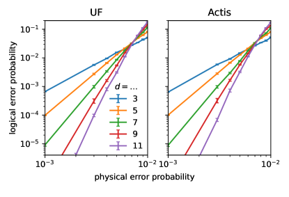
Figure 1: Threshold plots for original UF and Actis. We use the circuit-level noise model detailed in Appendix B. These numerics are consistent with the assertion in the main text that both decoders have the same accuracy. Each datapoint is the mean of $1\text{⋅}{10}^{4}1.5\text{⋅}{10}^{7}$ samples of decoding cycle; errorbars show standard error. The threshold is the physical error probability at which the lines cross, $\approx 7.5\text{⋅}{10}^{-3}$ for both plots.

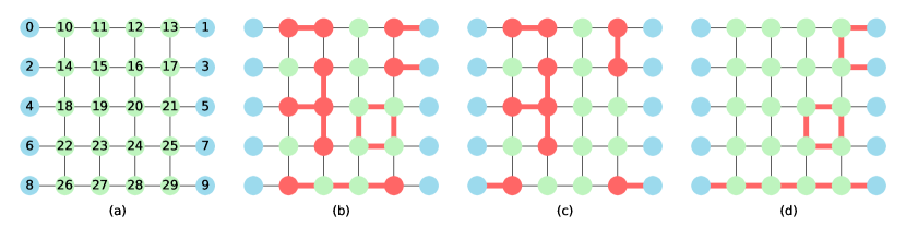
Figure 2: (a) The graph representing a distance-5 surface code. Detectors are green (nodes 10–29); boundary nodes, blue (nodes 0–9). (b) An example of an error $\mathbb{E}$ is the set of thick red edges whose corresponding syndrome $\mathbb{S}$ is the set of red nodes. Note a path in $\mathbb{E}$ (like that from node 26 to 29) will make a defect only at each endpoint; a cycle will make no defects. The decoder sees only $\mathbb{S}$, not $\mathbb{E}$. (c) A correction $\mathbb{C}$ for $\mathbb{E}$ is the set of thick red edges. The syndrome made by $\mathbb{C}$ is always the same as that of $\mathbb{E}$. (d) The leftover $\mathbb{L}$ after combining $\mathbb{E}$ and $\mathbb{C}$. This example comprises a cycle and two paths: one between nodes on the same boundary and one between opposite boundaries. The latter represents a logical bitflip.

Our main results extend this literature, especially the ideas proposed for Helios, as we introduce a paradigm which reduces the memory requirements of each node, the number and size of messages passed around, the grid architecture complexity, and the total number of algorithm stages. This enhancement, used in our version of almost-local UF called Macar, is a simple scheme inspired by anyon annihilation [22] to calculate parities. We also design Actis: a strictly local version of UF, the first of its kind, which is even more practical due to the lack of long-range links, and whose mean runtime is subquadratic in $d$ for error probabilities below threshold. While Helios was built only for phenomenological noise, we design our algorithms for circuit-level noise. Actis further takes advantage of the pre-existing decoder structure for this noise to minimise its physical overhead. Having compared Macar and Actis we note that the use of a fast communication relay implemented with asynchronous logic constitutes a third version of UF which rivals the speed of Macar whilst maintaining strict locality.

As well as having improved mean and worst-case runtime scalings, all three of our versions are exact implementations of, hence just as accurate as, original UF. We confirm the latter in Fig. 1, noting our versions behave identically in their output.

The paper proceeds as follows. In Section 2 we cover the prerequisite background theory. In Section 3 we discuss almost-local UF as introduced in the Helios scheme and our streamlined design, Macar, before describing our strictly local Actis in Section 4. We evaluate runtime for Macar and Actis in Section 5 and discuss how Actis can be sped up using asynchronous logic in Section 6. Section 7 concludes.

Our emulation code is on GitHub at [23] and the raw data for the plots in this paper is available at [24].

2 Background

Section 2.1 covers the surface code with a focus on decoding. We approach this standard material using graph theory as it facilitates a natural explanation of UF presented in Section 2.2.

2.1 Surface Code and Decoding

As its name suggests, the surface code arranges the physical qubits on a 2D grid. It encodes one logical qubit and corrects for both bit- and phaseflip errors (the ability to correct these two discrete errors allows us to correct any qubit error [25, §10.3.1]). Here, we describe how to correct bitflip errors; phaseflip errors are corrected analogously. We explain the decoding cycle under three noise models of increasing realism: code capacity, used in Section 2.1.1, assumes perfect measurements; phenomenological noise, described in in Section 2.1.2, generalises to faulty measurements. Section 2.1.3 discusses circuit-level depolarising noise.

2.1.1 Code Capacity

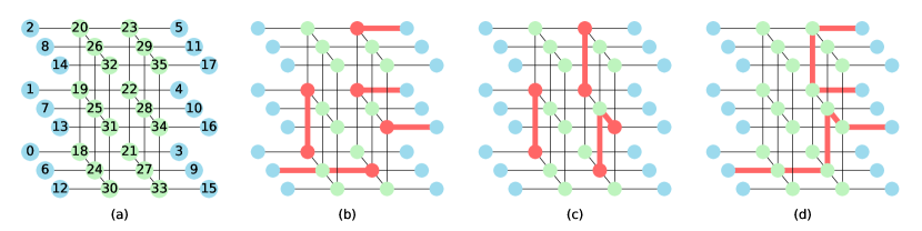
Figure 3: The 3D generalisation of Fig. 2 to account for faulty measurements. (a) Instead of distance-5, we show a distance-3 code for visual clarity. The time axis points upward. (b) The error $\mathbb{E}$ can now include vertical ‘timelike’ edges like that from node 18 to 19. The syndrome $\mathbb{S}$ is the set of red nodes throughout the whole lattice. (c) A correction $\mathbb{C}$ for $\mathbb{E}$. (d) The leftover $\mathbb{L}$ comprises one path between the same boundary and one between opposite boundaries. The latter represents a logical bitflip.

The surface code is based on the graph $G=(V,E)$ in Fig. 2(a) which comprises a set $V=V_{\textnormal{d}}\cup V_{\textnormal{b}}$ of nodes arranged on a $d\times(d+1)$ grid and a set $E$ of edges. Members of $V_{\textnormal{d}}$ are called detectors; $V_{\textnormal{b}}$, boundary nodes. Each edge corresponds to a set of two nodes from $V$. Physically, each detector represents an ancilla qubit used for measurement while each edge represents a data qubit. Boundary nodes represent nothing physical but exist just to allow every data qubit to be represented by an edge. We will treat the decoding problem abstractly in terms of nodes and edges. In a decoding cycle:

1. Noise corrupts our system Each edge bitflips with some probability $p$ called the physical error probability i.e. is assigned bit value 1 with probability $p$, and bit value 0 otherwise. The error $\mathbb{E}\subseteq E$ is the set of bitflipped edges.

2. Ancilla qubits flag the noise Every detector records the parity of the edges in $\mathbb{E}$ which are incident to it. If it records odd parity, it is a defect. The syndrome $\mathbb{S}\subseteq V_{\textnormal{d}}$ is the set of defects. Figure 2(b) shows an error and its syndrome. Mathematically, $\mathbb{S}=\sigma(\mathbb{E})$ where

   $$\sigma(\mathbb{E}):=V_{\textnormal{d}}\cap\operatorname*{{\triangle}}_{e\in\mathbb{E}}e$$ (1)

   and $\operatorname*{{\triangle}}_{e\in\mathbb{E}}e:=f\mathbin{\vartriangle}\dots\mathbin{\vartriangle}g$ for $\mathbb{E}=\{{f,\dots,g}\}$ where $\mathbin{\vartriangle}$ denotes symmetric difference.

3. The classical decoder acts Given $\mathbb{S}$, the decoder must output a correction $\mathbb{C}\subseteq E$ which, if treated as an error, would make the same syndrome $\mathbb{S}$. In other words, $\mathbb{C}$ must satisfy $\sigma(\mathbb{C})=\mathbb{S}$. Figure 2(c) shows a correction.

4. Success or failure The leftover $\mathbb{L:=E\mathbin{\vartriangle}C}$ is then guaranteed to satisfy the following lemma (for completeness, a proof is given in Section A.1).

   Lemma 1.

   $\mathbb{L}$ comprises only cycles or paths between distinct boundary nodes.

   The question of whether the decoder has been successful depends on whether a logical error has resulted from the correction. Any path between opposite boundaries represents a logical bitflip. Hence, if $\mathbb{L}$ has an odd number of such paths the logical qubit has picked up a logical error. Figure 2(d) shows a leftover with one such path.

The aim of the decoder is to output a correction which is least likely to lead to a logical error. Fig. 1 shows examples of how, for a surface code decoder, logical error probability depends on both $d$ and $p$. Each decoder has a different threshold i.e. physical error probability $p_{\textnormal{th}}$ below (above) which increasing $d$ decreases (increases) the logical error probability. The further below threshold a decoder operates, the more effective it is. In the case of UF, operating at its threshold is practically useless; significant benefits of error correction are reaped only when $p$ is several times below threshold i.e. $p\ll p_{\textnormal{th}}$.

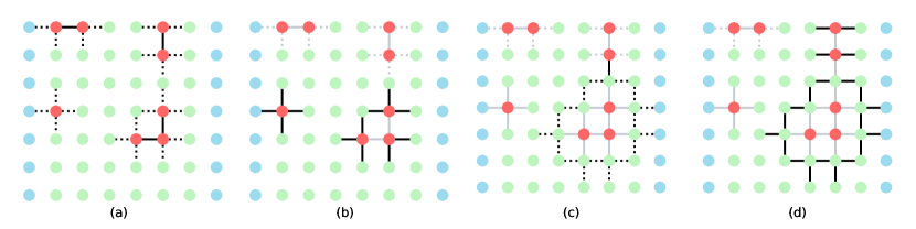
Figure 4: A syndrome validation example which needs four growth rounds. Ungrown edges are invisible; half-grown, dotted; fully grown, solid. Edges which have grown since the last round are black; else, grey. (a) Each defect grows its incident edges by $\frac{1}{2}$. Note some edges have grown by $\frac{1}{2}$ twice, so are fully grown. (b) The two active clusters grow again. The west one touches a boundary hence inactivates. (c) The remaining active cluster grows and touches hence merges with the inactive cluster north of it. (d) The resultant active cluster grows and touches the boundary hence inactivates.

2.1.2 Phenomenological Noise

In reality, ancilla qubit measurement is faulty i.e. in Item 2 each detector records the wrong parity with some probability $q$. The result is that the syndrome is subject to some noise: $\mathbb{S}=\sigma(\mathbb{E})\mathbin{\vartriangle}\mathbb{F}$, where $\mathbb{F}\subseteq V_{\textnormal{d}}$ is the set of nodes which record the wrong parity for that measurement round. Note boundary nodes cannot be in $\mathbb{F}$ as they do not represent ancilla qubits which are measured.

The usual way to account for faulty measurements is to measure each ancilla qubit not once but $\tau+1$ times per decoding cycle, where $\tau>0$ (intuitively, the higher $q$ is, the higher we should make $\tau$). We then have not one 2D sheet of syndrome data as in Fig. 2(b), but $\tau+1$ of them, which we label $\{{\mathbb{S}_{0},\dots,\mathbb{S}_{\tau}}\}$. In general there is a new $\mathbb{E}$ and $\mathbb{F}$ for each sheet, but the data is cumulative in $\mathbb{E}$ i.e.

$$\mathbb{S}_{t}=\big{[}{\operatorname*{{\triangle}}_{u=0}^{t}\sigma(\mathbb{E}_{u})}\big{]}\mathbin{\vartriangle}\mathbb{F}_{t}\qquad\forall t\in 0..\tau$$ (2)

so to localise each $\mathbb{E}_{t}$ we take the difference between consecutive sheets:

$$\textnormal{}\mathbb{S}_{t} :=\mathbb{S}_{t}\mathbin{\vartriangle}\mathbb{S}_{t-1}\qquad\forall t\in 1..\tau$$

$$\overset{\eqref{eq:2D_sheet}}{=}\sigma(\mathbb{E}_{t})\mathbin{\vartriangle}\mathbb{F}_{t}\mathbin{\vartriangle}\mathbb{F}_{t-1}.$$ (3)

We then stack these 2D ‘difference sheets’ $\{{\textnormal{}\mathbb{S}_{1},\dots,\textnormal{}\mathbb{S}_{\tau}}\}$ to make a 3D simple cubic lattice as in Fig. 3(a). Sheets are stacked such that $\textnormal{}\mathbb{S}_{1}$ is on the bottom, $\textnormal{}\mathbb{S}_{2}$ is the next one above, etc. This way, sheets which derive from later measurements are higher up the stack so we can interpret the upward direction as going forward in time (hence the subscript $t$).

Each detector no longer represents one ancilla qubit; rather, the difference between two consecutive measurements of that ancilla qubit at a given point in time. Each horizontal edge no longer represents one data qubit but a possible time at which that data qubit could bitflip. Vertical edges are a new addition: each one represents one possible faulty measurement. Specifically, each edge between $\textnormal{}\mathbb{S}_{t}$ and $\textnormal{}\mathbb{S}_{t+1}$ corresponds to a possible member of $\mathbb{F}_{t}$. This makes sense e.g. a member of $\mathbb{F}_{1}$ effects a change in both $\textnormal{}\mathbb{S}_{1}$ and $\textnormal{}\mathbb{S}_{2}$ as per Eq. 3.

If we redefine $G$ as this 3D simple cubic lattice, all steps of the decoding cycle are the same as in Section 2.1.1 with the modification in Item 1 that each horizontal edge bitflips with probability $p$; each vertical edge, $q$. Detectors still always record the correct parity as now faulty measurements are modelled by vertical edges. Figure 3(b–d) shows a decoding cycle example.

In our emulations we assume the batch decoding scheme i.e. we set $\mathbb{F}_{0}=\mathbb{F}_{\tau}=\varnothing$, which explains the absence of vertical edges below $\textnormal{}\mathbb{S}_{1}$ and above $\textnormal{}\mathbb{S}_{\tau}$ in Fig. 3. This simplification allows us to determine the success of the decoder for a batch of $\tau+1$ measurement rounds in isolation. In contrast, continuously decoding a constant stream of syndrome data from an indefinite number of measurement rounds is the topic of stream decoding. We do not treat this in our paper as methods already exist allowing most batch decoders, including our versions of UF, to be used as stream decoders [1, 26, 27].

2.1.3 Circuit-Level Noise

Yet a more realistic noise model is the circuit-level depolarising model, which considers the quantum circuit performed during a measurement round and a variety of possible faults it can make. Details of this are provided in Appendix B but the end result is the addition of certain diagonal edges in $G$, as Fig. 11(a) shows. The bitflip probability for each edge is a function of some characteristic physical error probability $p$; this function potentially varies for each edge.

Circuit-level noise depends on parameters not standardised in literature so it is difficult to compare thresholds under this model. This is not the case for code capacity and phenomenological noise (standardised by setting $q=p$ and $\tau=d$), under which we numerically obtain thresholds for UF of $\approx 9.8\text{⋅}{10}^{-2}$ and $\approx 2.6\text{⋅}{10}^{-2}$ respectively, consistent with previous results [28, §5.4].

MWPM is a popular decoder which finds a most likely error for the syndrome, and outputs that as the correction i.e. $\mathbb{C}=\arg\max\{{\operatorname{pr}(\mathbb{E}):\sigma(\mathbb{E})=\mathbb{S}}\}$. For small $p$ under code capacity or standardised phenomenological noise, this amounts to finding a correction whose size $|\mathbb{C}|$ is minimal. While accurate, MWPM has a worst-case runtime $\mathcal{O}(N^{3}\lg N)$ [29, §3] where $N:=|V|=\mathcal{O}(d^{2})$ for code capacity and $\mathcal{O}(d^{3})$ for the other noise models. UF approximates MWPM [30] with an improved worst-case runtime $\mathcal{O}\big{(}{N\alpha(N)}\big{)}$ where $\alpha(N)\leq 3$ for all practical $d$. In Appendix C we compare the accuracy of MWPM with UF for practical noise levels and discuss their near-term relevance.

For visual clarity, Figs. 4 to 10 use $G$ for code capacity. However, the reader should keep in mind the rest of the paper (save Section 4 which focuses on circuit-level noise) also applies to the other noise models.

2.2 UF

Conceptually, UF groups defects into spatial clusters then finds a correction only from edges within a cluster. UF keeps the total size of all clusters small to ensure the correction is small. The algorithm comprises the following stages:

1. Syndrome Validation An active cluster nucleates at each defect which grows outward in all directions at the same speed.

2. Spanning Forest Growth A spanning tree is grown within each cluster. Using our parity-calculation scheme, this stage comes for free.

3. Peeling Each edge of each tree is peeled i.e. removed from the tree and included or excluded from the correction depending on the syndrome.

2.2.1 Syndrome Validation

Figure 4 shows a syndrome validation example. Mathematically, a cluster $C=(V_{C},E_{C})$ is a connected subgraph of $G$. A cluster is active iff there exists no correction for its defects using only edges in the cluster i.e. $\nexists\mathbb{C}\subseteq E_{C}:\sigma(\mathbb{C})=\mathbb{S}\cap V_{C}$. Else it is inactive. Intuitively, an inactive cluster is one where we have accounted for all defects with a correction local to that cluster; an active cluster still seeks such a correction. In practice we determine activity by the following lemma adapted from [20, Lemma 1] and proved in Section A.2.

Lemma 2.

Cluster $C$ is active iff it has an odd defect count and touches no boundary i.e.

$$\big{(}{\textnormal{$|\mathbb{S}\cap V_{C}|$ odd}}\big{)}\wedge\big{(}{V_{\textnormal{boundary}}\cap V_{C}=\varnothing}\big{)}.$$ (4)

Before syndrome validation, a cluster $(\{{v}\},\varnothing)$ is initialised for every $v\in V$ (so there is an active cluster for each defect and an inactive one for each nondefect). Each edge in $E$ has a growth value in $\{{0,\frac{1}{2},1}\}$ which is initialised at 0. Syndrome validation proceeds via some number of growth rounds and stops when all clusters are inactive. In a growth round:

1. Each active cluster grows all edges around it by $\frac{1}{2}$.

2. Each new fully grown edge merges the two clusters at its endpoints into one bigger cluster, if the endpoints did not already belong to the same cluster. Mathematically, if clusters $A$ and $B$ merge along edge $e$ the resultant cluster is

   $$C=\big{(}{V_{A}\cup V_{B},E_{A}\cup E_{B}\cup\{{e}\}}\big{)}.$$ (5)

One may wonder why edges grow by only $\frac{1}{2}$ per growth round. If they grew by 1 per round, a pair of defects separated by two edges would merge just as fast as a pair separated by one edge. Growing edges by $\frac{1}{2}$ per round distinguishes these cases, reducing the number of fully grown edges hence the size of all clusters.

Syndrome validation has a runtime $\mathcal{O}\big{(}{N\alpha(N)}\big{)}$ if the Union–Find data structure (after which the Union–Find decoder is named) is used [31]. It ensures the existence of a correction using only cluster edges while the next two stages, shown in Fig. 5, find an instance of one.

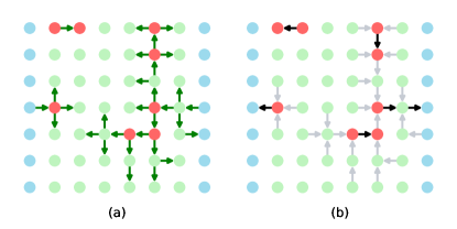
Figure 5: Continuing the example in Fig. 4: (a) A spanning forest is grown in the direction of the arrows. Each arrow is an edge in the forest and points from parent to child node. (b) The forest is peeled in the direction of the arrows. The set of black arrows is the correction returned by the decoder.

2.2.2 Spanning Forest Growth

For each cluster $C$ a root node is chosen as follows: if $C$ touches a boundary, one of its boundary nodes is chosen; else, any node is chosen. A spanning tree of $C$ (a subgraph of $C$ that is connected, acyclic, and spans $V_{C}$) is then grown from this root. The union of all the trees is the forest. This stage is done by breadth- or depth-first search; either way, the runtime is linear in the number of edges in the forest i.e. $\mathcal{O}(N)$.

2.2.3 Peeling

A correction $\mathbb{C}=\varnothing$ is initialised then the forest is traversed edge by edge, starting from the leaves. Each time a defect is encountered all edges traversed thereafter, until another defect is encountered, are added to $\mathbb{C}$. Once the whole forest has been traversed $\mathbb{C}$ will satisfy $\sigma(\mathbb{C})=\mathbb{S}$ [19, Theorem 1]. Since each edge in the forest is traversed exactly once the runtime is $\mathcal{O}(N)$.

2.2.4 Weighted Edges

Under phenomenological and circuit-level noise, the bitflip probability may vary for each edge. In the case these probabilities are known, UF can be made more accurate by modifying syndrome validation to grow clusters along weighted edges i.e. whose growth values are more granular than $\{{0,\frac{1}{2},1}\}$ [32].

This concludes our review of the well-established surface code and UF paradigms, using the notation that we require for the remainder of the paper. We now briefly discuss recent literature working towards local architectures for implementing UF, especially Helios.

3 Almost-Local UF

It is clear the nature of UF is quite local: all edges involved connect neighbouring nodes, and two clusters communicate only when they touch; so it seems sensible to implement UF as locally as possible. This may have advantages over the standard picture in which the decoder protocol is implemented using a single, fully fledged classical processor, located remotely from the actual qubits. Instead, one can imagine a more distributed decoder comprising a very simple classical processor corresponding to each node and an interprocessor communication link corresponding to each edge. We can visualise this local architecture as directly corresponding to Fig. 11(a) if nodes represent processors and edges represent the links.

This alternative paradigm has various benefits. Firstly, its computation is parallelised: non-neighbouring computations can be run independently and simultaneously; we will see this leads to superior runtime scaling. Secondly, it allows each processor to sit closer to its data source (the ancilla qubit), simplifying wiring and reducing signal losses [33, p $67$]. Thirdly, there may be implications in terms of robustness: if one part breaks down then only that part, rather than the whole decoder, must be replaced.

In Section 3.1 we give a conceptual overview of Helios developed by Liyanage et al. [21] and in Section 3.2 we describe Macar in detail, including our parity-calculation scheme that simplifies the physical architecture and allows a spanning forest to be grown in one timestep regardless of $d$.

3.1 Helios

The authors consider only syndrome validation as this is the only stage that is nontrivial to implement locally. Their implementation uses the local architecture just described i.e. there is a processor for each node in $G$ and a communication link for each edge. For the rest of this section we refer to processors as nodes and communication links as edges.

Clusters are identified by a unique integer stored by all its nodes. When two clusters merge the higher-integer cluster becomes part of the other one. This occurs via a flooding algorithm: each node looks at its neighbours along fully grown edges; if it sees a lower integer than its own, it stores that lower integer instead. This results in a wave of change propagating across the higher-integer cluster, starting from where the two clusters touched. After the flood, all the nodes of the higher-integer cluster will store the lower integer. Generalising to three or more clusters merging at once is simple: a flood propagates from each touching point but eventually only the lowest-integer cluster will remain.

As well as merging, the other task in syndrome validation is determining the activity of each cluster. The authors devised the following messaging system to tackle this. Each cluster always has a well-defined root node. Whenever a defect changes its stored integer, it sends a message to the root of the cluster it has just joined. Every root stores a bit and flips it whenever it receives a message. Once all flooding has finished and all messages have reached their destination, the bit of each root will equal its cluster’s defect count parity. This, by 2, determines the activity of clusters which do not touch a boundary. The authors do not mention treatment of clusters which touch a boundary but we do so in Section 3.2.1. These messages are sent via a network comprising the edges of $G$ and additional edges between non-neighbouring nodes but our modification removes the need for them.

In addition to the nodes, there is a central controller which manages the global variables of the UF algorithm. It connects to each node via a hierarchical tree which allows restricted communication: the controller can broadcast the same message to all nodes and receive Boolean messages from any node, but does not know the sender. This is why we say Helios is almost local. The authors leave tree height as a design choice; in this paper we follow their implementation, suitable for low code distances, and set it to 1 i.e. connect the controller directly to each node. This allows us to ignore the time cost of controller–node communication.

In this limit, the worst-case runtime of Helios is $\mathcal{O}(N)$ as the maximum possible cluster diameter (defined for a graph as the maximum length of a shortest path) is $\mathcal{O}(N)$ and the duration to flood such a cluster (example in Fig. 6)

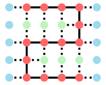
Figure 6: A maximum-diameter cluster is a winding snake-like path of length $\mathcal{O}(N)$ where $N$ is the number of nodes in the graph $G$.

scales linearly with its diameter. This is formally better than the $\mathcal{O}\big{(}{N\alpha(N)}\big{)}$ of original UF owing to the parallelism of Helios. More impressive is the mean runtime which, for phenomenological noise i.e. $N=\mathcal{O}(d^{3})$, the authors report as sublinear in $d$ from numerics.

3.2 Macar

We assume decoding to be cellular automata-like i.e. via discrete timesteps with each component performing one operation, and messages travelling one edge, per timestep.

The controller has a variable attribute stage indicating which stage it is in. It is initialised to growing and follows the flowchart in Fig. 7.

Figure 7: Flowchart for the stage variable which alternates between fixed- and arbitrary-duration stages.

There are seven stages: growing, merging, presyncing, syncing, burning, peeling, done. The odd stages last exactly one timestep; the even stages, an arbitrary number of timesteps. During syndrome validation the controller cycles through the first four stages once per growth round. burning is for spanning forest growth, peeling is for peeling, and done indicates the end of the decoding cycle.

Algorithm 1 Run by controller every timestep.

AdvanceMacarController $(\text{not}~{}v.\texttt{busy})~{}\forall v\in V$$\texttt{stage}=\texttt{syncing}$$(\text{not}~{}v.\texttt{active})~{}\forall v\in V$

$\texttt{stage}\leftarrow\texttt{burning}$

$\texttt{stage}\leftarrow\texttt{growing}$

$\texttt{stage}\leftarrow$ next stage $\triangleright$ Stage order is as introduced in Section 3.2.

Algorithm 2 The four procedures each node can run during syndrome validation.

Growing$v$$v.\texttt{active}$unfully grown edges $e$incident to $v$

$e.\texttt{growth}\leftarrow e.\texttt{growth}+\frac{1}{2}$

Merging$v$

$v.\texttt{busy}\leftarrow\texttt{false}$ ($v\in V_{\textnormal{d}}$) and ($v$ not a root) and ($v.\texttt{anyon}$)

$v.\texttt{busy}\leftarrow\texttt{true}$

relay anyon in direction of $v.\texttt{pointer}$ $u\in\operatorname{access}v$ $u.\texttt{CID}<v.\texttt{CID}$

$v.\texttt{busy}\leftarrow\texttt{true}$

$v.\texttt{pointer}\leftarrow$ toward $u$

$v.\texttt{CID}\leftarrow u.\texttt{CID}$

Presyncing$v$

$v.\texttt{active}\leftarrow$ ($v\in V_{\textnormal{d}}$) and ($v$ a root) and ($v.\texttt{anyon}$)

Syncing$v$

$v.\texttt{busy}\leftarrow$ (not $v.\texttt{active}$) and ($\exists u\in\operatorname{access}v:u.\texttt{active}$)

$v.\texttt{active}\leftarrow v.\texttt{active}$ or $v.\texttt{busy}$

Each node $v\in V$ is assigned a unique integer ID as in Fig. 11(a) and has the following variable attributes:

• defect is a boolean indicating whether $v\in\mathbb{S}$.

• active is a boolean indicating whether the cluster that $v$ is in is active. Since $v$ starts in its own cluster, $v.\verb|active|$ is initialised as $v.\verb|defect|$. If $v.\verb|active|=\verb|true|$ we say $v$ is active.

• CID is an integer indicating the cluster that $v$ belongs to. Clusters are identified by the lowest ID of all its nodes. The node of this ID is the root of the cluster. Since $v$ starts in its own cluster, $v.\verb|CID|$ is initialised as $v.\verb|ID|$.

• anyon is a boolean indicating whether $v$ has an anyon. This anyon can be thought of as a particle which is passed between nodes during syndrome validation. When two anyons meet i.e. a node receives two anyons in a timestep, they annihilate. $v.\verb|anyon|$ is initialised as $v.\verb|defect|$. The idea is to accumulate at the root all the anyons in a cluster so they annihilate on the way or on arrival. Eventually zero or one anyon will remain at the root, indicating the cluster’s defect count parity.

• pointer is the direction $v$ should relay the anyon. Possible values (under circuit-level noise) are C, N, W, E, S, D, U, NU, WD, EU, SD, NWD, SEU, representing respectively centre, north, west, east, south, down, up, and combinations thereof. Following the pointers starting from $v$ should eventually lead to the root of the cluster that $v$ is in. Only roots have $\verb|pointer|=\verb|C|$ as they do not relay anyons but accumulate them. $v.\verb|pointer|$ is initialised to C. Together, anyon and pointer replace Helios’ messaging system.

• busy is a boolean used to indicate whether $v$ is busy. $v.\verb|busy|$ is initialised to false.

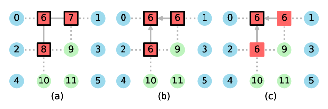
Figure 8: An example of a merging stage which needs three timesteps. Active nodes are square-shaped; inactive nodes are circular. CID is shown as a label. Nodes with anyons are outlined in black. Pointers are shown by arrows on edges. (a) The first growth stage has just finished. (b) Nodes 7 and 8 change their CID to 6 and point to node 6 which is now the root of a three-node cluster. (c) Nodes 7 and 8 relay their anyons to the root; the two anyons annihilate and one remains, indicating the cluster’s defect count is odd. This cluster touches no boundary so by 2 is active.

Each edge has a variable attribute growth equal to its growth value, initialised as $0~{}\forall e\in E$. We restrict growth values to $\{{0,\frac{1}{2},1}\}$ and leave granularising for future work, but allow UF under circuit-level noise to grow along the diagonal edges as we found this gave a $1.5\times$ improvement to the threshold. Since processing is done at nodes rather than edges we can for each edge pick one of its endpoints, say the one of the lower ID, to be responsible for storing its growth. The set of edges a node is responsible for, is then the owned edges

$$v.\texttt{owned}:=\{{uv:uv\in E~{}\text{and}~{}v.\texttt{ID}<u.\texttt{ID}}\}$$ (6)

stored as a constant attribute.

In each timestep the controller runs Algorithm 1, which simply moves stage on if no node is busy. This is where the controller–node connectivity is used: the controller need not know which node is busy; rather, if a node is busy. After every syncing stage the controller also checks for any active clusters. If there are, another growth round is needed so stage is reset to growing. If none, syndrome validation is done so stage is set to burning.

Once stage reaches done the controller stops running Algorithm 1 and the decoder outputs the correction $\mathbb{C}$ made during peeling. In this paper we do not consider how the decoder offloads $\mathbb{C}$ and loads in the next $\mathbb{S}$ as these are topics more relevant to stream decoding.

3.2.1 Syndrome Validation

It is helpful to define the access of a node as the set of neighbours along fully grown edges:

$$\operatorname{access}v:=\{{u\in V:uv\in E\wedge uv.\texttt{growth}=1}\}.$$ (7)

In a timestep each node runs whichever procedure matches stage out of the four in Algorithm 2.

Stage growing is simply a change of growths: each node in an active cluster increments the growth of edges around it, if not already fully grown.

Figure 8 shows a merging example. In merging two processes occur: flooding and anyon annihilation. Flooding is as described in Section 3.1: each node looks at its access; if it sees a lower CID than its own, it updates its own to match it. Additionally, the node updates its pointer toward that neighbour. This ensures following the pointers always leads to the correct root promised by CID. In anyon annihilation, any node with an anyon relays it in the direction of its pointer. At the end of this stage, a cluster’s defect count is odd iff its root has an anyon.

Ideally, pointers are updated before anyons are relayed. However, the practicality of this depends on the hardware implementation so in this paper we assume the worse case and relay anyons in the direction of pointers from the previous timestep.

Stage presyncing determines which clusters are active. Note in Fig. 2(a) boundary nodes are of lower ID than detectors. This ensures that if a cluster touches a boundary, its root is a boundary node. Each root can thus determine if its cluster is active by checking if itself is a boundary node and if it has an anyon, by 2. In presyncing, roots of active clusters set their active attribute to true; every other node sets theirs to false.

Figure 9 shows a syncing example.

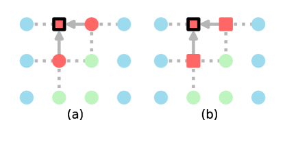
Figure 9: An example of a syncing stage which needs two timesteps. Attributes are shown as in Fig. 8 but without CID. (a) A presyncing stage has just finished. Note how the only active node is the root of the three-node active cluster. (b) Nodes 7 and 8 see this active node along a fully grown edge so become active themselves. This is the end of the flood as all the nodes in the active cluster are active.

Algorithm 3 Run by each node during burning.

Burning$v$$uv\in v.\texttt{owned}$$uv.\texttt{growth}=1$and not ($u.\texttt{pointer}$toward $v$or $v.\texttt{pointer}$toward $u$)

$uv.\texttt{growth}\leftarrow 0$

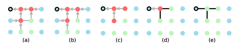
Figure 10: An example of burning and peeling. Attributes are shown as in Fig. 9. (a) Before burning, a cluster contains a cycle, which has one edge no pointer points along. (b) This edge is burned i.e. removed to leave behind a spanning forest. (c) The four leaves of the forest are peeled resulting in a smaller forest. (d) The two leaves of the smaller forest are peeled resulting in an even smaller forest. These two edges are added to the correction because the leaf nodes were defects. Edges so far added to the correction are in black. (e) The final leaf is peeled and added to the correction.

In syncing the activity of each cluster is propagated from root to all its other nodes via a flood: each node looks at its access; if it sees an active node, it becomes active, if not already. At the end of this stage, a node is in an active cluster iff it is active.

In Helios’ messaging system, messages contain the ID of the destination node. The memory needed to store this scales logarithmically in $d$. A new message is emitted whenever a defect changes its CID which leads to $\mathcal{O}(N^{2})$ messages throughout syndrome validation in the worst case. Messages must be kept separate so buffers are needed but these can stall if full. Anyon annihilation improves upon this system as anyon is one bit regardless of $d$. Throughout syndrome validation, the anyon count never exceeds the defect count in $G$ and only ever decreases, so is $\mathcal{O}(N)$ in the worst case. There is no need for buffers (as anyons need not be kept separate) nor additional links between non-neighbouring nodes.

3.2.2 Burning

In original UF a spanning forest is grown in $\mathcal{O}(N)$ timesteps via breadth- or depth-first search. Macar does this in one timestep by retrieving the forest directly from the pointers in a stage we call burning, described in Algorithm 3. Figure 10(a, b) shows an example. In burning, any fully grown edge no pointer points along is ‘burned’ i.e. sets its growth to 0. The spanning forest is the set of fully grown edges which remain. This is because the pointers already define a spanning tree within each cluster; burning simply removes the edges ‘unused’ by these pointers.

3.2.3 Peeling

Figure 10(b–e) shows how peeling is done in Macar; this is simply a local version of that described in Section 2.2.3 and takes $\mathcal{O}(N)$ timesteps. In a timestep each node runs the procedure in Algorithm 4: each node checks if it is a leaf node of the spanning forest; if so it will peel its corresponding leaf edge.

Algorithm 4 Run by each node during peeling.

Peeling$v$

$v.\texttt{busy}\leftarrow\texttt{false}$ ($v$ not a root) and $\big{(}{|{\operatorname{access}v}|=1}\big{)}$

2:$v.\texttt{busy}\leftarrow\texttt{true}$

$\{{u}\}:=\operatorname{access}v$

4:$uv.\texttt{growth}\leftarrow 0$ $v.\texttt{defect}$

$v.\texttt{defect}\leftarrow\texttt{false}$

6:add $uv$ to $\mathbb{C}$

flip $u.\texttt{defect}$

3.2.4 Runtime

Macar’s worst-case decoding runtime is $\mathcal{O}(N)$ due to the same reason as Helios’: flooding a cluster of diameter $\mathcal{O}(N)$ is the process with the worst scaling in the whole decoding cycle. Specifically, the maximum number of timesteps to flood a cluster equals its diameter. Section 5 shows the mean runtime scales similarly to Helios’ as expected.

4 Actis

In this section we focus on circuit-level noise and present a strictly local UF i.e. one without a direct communication link between the controller and each node. Instead, the controller communicates only with the node of ID 0. Broadcasting of stage from controller to nodes happens via a global flood, and busy and active propagate as signals from node to controller by relaying.

These two new processes, which we call staging and signalling respectively, are communicated through the local tree $T_{\text{SS}}$ shown in Fig. 11(b).

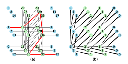
Figure 11: (a) The generalisation of Fig. 3(a) to circuit-level noise. The diagonal edges exist in every cubelet in the bulk of $G$. The thick red path is an example of a logical bitflip. (b) The tree $T_{\text{SS}}$ used in Actis, with nodes labelled by their span. Each edge tapers toward the parent.

Signalling is similar to how anyons are relayed but instead of following variable pointers, these signals follow constant pointers toward the controller, traversing one edge in $T_{\text{SS}}$ per timestep. This requires the controller and nodes to store additional attributes which are described in Section 4.2.

The change clearly increases runtime but has the advantage of lacking long-range links, so is an even lower stepping stone toward practicality. The worst-case runtime remains $\mathcal{O}(N)$ and is discussed in Section 4.4. We will see in Section 5 the mean runtime is below $\mathcal{O}(d^{2})$ for all practical noise levels. Moreover we note that a rapid-transmission variant can substantially recover the speed of Macar within the strictly local paradigm.

4.1 The Staging and Signalling Tree

As Fig. 11(b) shows, the root of $T_{\text{SS}}$ is node 0. Its height i.e. distance from root to a furthest node, equals the code distance: $h(T_{\text{SS}})=d$. Almost all edges in $T_{\text{SS}}$ are diagonals which already exist in $G$ for circuit-level noise. The only additional edges are in the west, east, and lower faces of $G$, whose count is $\mathcal{O}(d^{2})$ compared to $\mathcal{O}(d^{3})$ for edges in $G$. Therefore the physical overhead of $T_{\text{SS}}$ is low.

$T_{\text{SS}}$ differs from the hierarchical tree of Helios’ controller: $T_{\text{SS}}$ is mostly embedded in $G$ and is truly local, unlike the latter which is separate from $G$ and intersects $V$ only at its leaves.

4.2 Additional Attributes

The controller stores a constant integer $\texttt{span}=1+h(T_{\text{SS}})$ and has the following variable attributes:

• countdown is an integer which tracks how long the controller must wait until it is sure staging or signalling is done. It is initialised to 0.

• busy_signal is a boolean indicating whether the controller receives a busy signal in the current timestep.

• active_signal is a boolean indicating whether the controller has received an active signal during the current syncing stage. It is initialised to false.

Each node $v\in V$ stores the following constants:

• $\texttt{span}=h(T_{\text{SS}})-\operatorname{depth}v$, where $\operatorname{depth}v$ is the distance in $T_{\text{SS}}$ from $v$ the root.

• signalee is the parent of $v$ in $T_{\text{SS}}$ i.e. the neighbour in the direction toward the controller. This is the neighbour that $v$ looks to for staging, and sends busy and active signals to. For node 0, signalee is the controller.

Each node $v$ also has the following variable attributes:

• stage is used for staging; possible values are the seven stages. $v.\verb|stage|$ is initialised to growing.

• countdown is same as that of controller but used only to track how long $v$ must wait until staging is done. $v.\verb|countdown|$ is initialised to 0.

• busy_signal is a boolean indicating if in the current timestep, $v$ either is busy or receives a busy signal from another node.

• active_signal is a boolean indicating if in the current timestep, $v$ either has stage as presyncing and becomes active, or receives an active signal from another node.

To manage these additional attributes the procedures have additional steps, explained in the next subsection.

Algorithm 5 Run by controller every timestep in Actis.

AdvanceLocalController $\texttt{countdown}=0$stagechange block. $\texttt{stage}=\texttt{syncing}$not active_signal

$\texttt{stage}\leftarrow\texttt{burning}$

2:$\texttt{stage}\leftarrow\texttt{growing}$

$\texttt{stage}\leftarrow$ next stage countdown reset block. $\texttt{stage}\in\{{\texttt{merging},\texttt{peeling}}\}$

4:$\texttt{countdown}\leftarrow\texttt{span}+1$

$\texttt{countdown}\leftarrow\texttt{span}$ busy_signal and $\texttt{countdown}\leq 2$

6:$\texttt{countdown}\leftarrow 2$ $\triangleright$ Only occurs during arbitrary-duration stages.

$\texttt{countdown}\leftarrow\texttt{countdown}-1$

Algorithm 6 Each node in Actis runs AdvanceLocalNode every timestep.

AdvanceLocalNode$v$

$\Call{Proc}{}\leftarrow$ procedure matching $v.\texttt{stage}$ in Algorithms 2, 3 and 4 $v.\texttt{stage}\in\{{\texttt{merging},\texttt{syncing},\texttt{peeling}}\}$

2:AdvanceArbitrary$v$, Proc

AdvanceFixed$v$, Proc

4:AdvanceFixed$v$, Proc $\triangleright$ For fixed-duration stages. $v.\texttt{countdown}=0$

Proc$v$ $v.\texttt{stage}=\texttt{presyncing}$

6:$v.\texttt{active\_signal}\leftarrow v.\texttt{active}$

$v.\texttt{stage}\leftarrow$ next stage

8:$\texttt{countdown}\leftarrow\texttt{countdown}-1$

AdvanceArbitrary$v$, Proc $\triangleright$ For arbitrary-duration stages. $v.\texttt{stage}=v.\texttt{signalee}.\texttt{stage}$

10:Proc$v$

$v.\texttt{busy\_signal}\leftarrow v.\texttt{busy\_signal}$ or $v.\texttt{busy}$

12:relay $v.\texttt{busy\_signal}$ and $v.\texttt{active\_signal}$ to $v.\texttt{signalee}$

$v.\texttt{stage}\leftarrow v.\texttt{signalee}.\texttt{stage}$ $\triangleright$ Staging.

14:$v.\texttt{countdown}\leftarrow v.\texttt{span}$

4.3 Modified Procedures

For the controller, Algorithm 1 is replaced by Algorithm 5. Main differences are: checking for any busy nodes is replaced by checking if countdown has reached 0; checking for any active nodes, by checking if an active signal has been received.

For Macar the four stages that lasted one timestep each followed an arbitrary-duration stage, so in Actis, staging must be used to broadcast these four stages to all nodes. As indicated in 5, staging lasts span timesteps: the duration for a stage flood to propagate from controller to the furthest nodes. Hence these four stages are still of fixed duration (for fixed $d$).

The other three (arbitrary-duration) stages need not be broadcast as they each follow a fixed-duration stage so all nodes know exactly when to start them. In merging and peeling the controller must wait at least $\verb|span|+1$ timesteps as it takes span timesteps for a signal to go from a furthest node to the controller. 4 indicates this. In syncing the furthest nodes are never busy nor active (all are boundary nodes) so the controller need only wait at least span timesteps (5). In any of these three stages, after this minimum duration, busy signals are no more than two edges apart due to 1 so countdown resets to 2 in 6.

Proposition 1 (Doppler effect).

For any busy signal received by the controller after $\verb|span|+1$ timesteps in merging, another busy signal must have been received $\leq 2$ timesteps earlier.

Proof.

All busy signals emitted in the first merging timestep reach the controller in $\verb|span|+1$ timesteps or less. Hence any busy signal $s$ received after this time must have been emitted by some node $v$ at some time $t_{s}$ after the first merging timestep. This implies at $t_{s}-1$ some node $u\in\{{v}\}\cup\operatorname{access}v$ was busy, so emitted a busy signal $s^{\prime}$. The duration between the controller receiving $s^{\prime}$ and $s$ is maximised when $u$ is 1 edge closer to the controller than $v$. In this case $s^{\prime}$ arrives 2 timesteps before $s$. ∎

The proof of 1 can be understood as a Doppler effect: waves of busyness travel through clusters at a speed of one edge per timestep. Wavefronts emit busy signals at a frequency of once per timestep. If a wave travels away from the controller, the controller will receive these signals at a frequency of once per two timesteps.

In a timestep each node runs AdvanceLocalNode in Algorithm 6. This reuses Algorithms 2, 3 and 4 but wraps each procedure in either AdvanceFixed or AdvanceArbitrary depending on whether the stage is of fixed or arbitrary duration.

A node’s countdown is used only when its stage is of fixed duration, during which it should equal the controller’s countdown. It tells the node exactly when to change stage: as soon as it reaches 0 in 4. At other times i.e. after arbitrary-duration stages, the update of stage occurs via staging (13).

4.4 Worst-Case Runtime

The new processes in Actis, staging and signalling, take $\mathcal{O}(d)$ timesteps and are used $\mathcal{O}(1)$ times per growth round. A decoding cycle needs a maximum of $\mathcal{O}(d)$ growth rounds so these processes contribute a maximum $\mathcal{O}(d^{2})$ timesteps to the overall runtime. Hence the worst-case runtime scaling of Actis remains $\mathcal{O}(N)$, where $N=\mathcal{O}(d^{3})$ for circuit-level noise.

5 Runtime Analysis

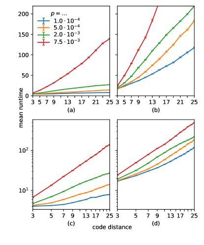
Figure 12: Syndrome validation runtime against code distance, under circuit-level noise for different physical error probabilities $p$. Each datapoint is the mean of $1\text{⋅}{10}^{3}$ samples of decoding cycle; errorbars show standard error. (a) Macar. (b) Actis. (c, d) same as (a, b) but on a log–log scale.

We wrote a Python package [23] implementing original UF, Macar and Actis. We then tested the runtimes of Macar and Actis by emulating a decoding cycle under circuit-level noise and counting the number of timesteps to complete syndrome validation. This is a good proxy for decoding runtime as we already know the exact runtime of burning, and peeling is never slower than the last round of merging.

Remark.

burning and peeling need not be standalone stages. We could have incorporated peeling into merging if, instead of relaying an anyon along an edge, we peeled that edge, with the modifications in Algorithm 4 that 4 is not done and 6 becomes $\mathbb{C}\leftarrow\mathbb{C}\mathbin{\vartriangle}\{{uv}\}$. Defects would then take over the role of anyons and the decoding cycle would finish after the last syncing stage, without need for burning. Although small, this modification may be useful in future implementations for which we want to minimise the number of stages e.g. a local UF stream decoder.

Note the runtimes we record are for correcting only bitflips. The full decoding cycle in practice requires two copies of the decoder: one for each error type (bit- and phaseflip). Since these copies can operate simultaneously the overall runtime is always the slower of the two. The runtimes presented here are thus to be interpreted as raw, as they demonstrate the scaling of the fundamental algorithm but are not subject to the above effect.

Figure 12 shows the mean runtime of Macar and Actis. We use this data to estimate in Table 1 the scaling $m$, assuming mean runtime $\propto d^{m}$.

Table 1: Gradient $m$ of the lines in Fig. 12(c, d) estimated using Weighted Least Squares.

$p$	Macar	Actis
$1.0\text{⋅}{10}^{-4}$	0.27(3)	0.77(3)
$5.0\text{⋅}{10}^{-4}$	0.55(3)	1.04(4)
$2.0\text{⋅}{10}^{-3}$	0.86(1)	1.19(2)
$7.5\text{⋅}{10}^{-3}$	1.48(1)	1.46(2)

As $\approx 7.5\text{⋅}{10}^{-3}$ is the threshold of UF, $2.0\text{⋅}{10}^{-3}$ is roughly the highest practical $p$ at which UF would operate. For this value of $p$ and below: Macar shows sublinear scaling; Actis, subquadratic scaling. We expect the former as Macar is closely related to Helios which scales sublinearly [21]. Note we implement Macar with a hierarchical tree height of 1 to isolate the behaviour of Algorithm 2, though such a tree is not scalable in $d$. Runtimes for any scalable implementation of Macar would incur an extra $\mathcal{O}(\lg d)$ contribution to those presented here due to a height-$\mathcal{O}(\lg N)$ tree.

We also evaluate runtime distribution, shown in Fig. 13.

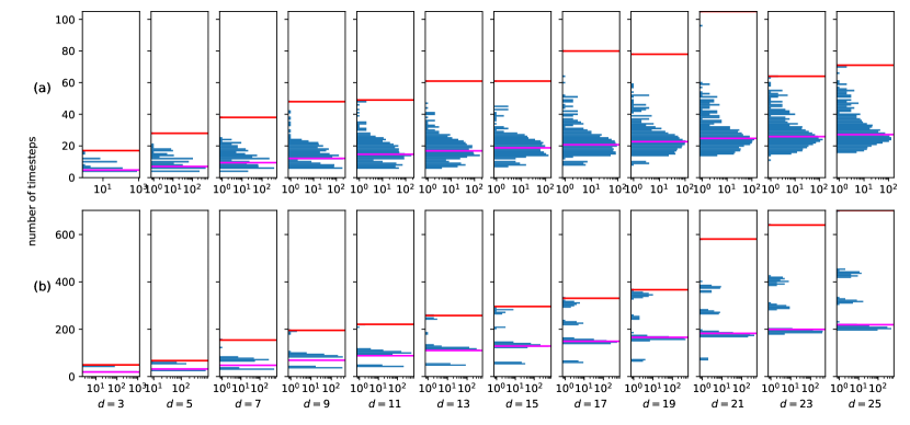
Figure 13: Syndrome validation runtime for physical error probability $p=$2.0\text{⋅}{10}^{-3}$$. Within each histogram: the horizontal magenta line shows the mean; red line, the maximum, of $1\text{⋅}{10}^{4}$ samples of decoding cycle. (a) Macar; each bar has width 1. (b) Actis; each bar has width 6.

Actis has equally spaced sharp peaks in runtime; each one corresponds to one growth round. The wide spacing implies most of its runtime is due to staging and signalling i.e. the controller waiting until countdown reaches 0 before moving on [this can also be inferred by the difference in absolute runtime between Macar and Actis: at $d=25$ the former is 8.06(9) times faster than the latter].

The peak locations can be derived as follows. If syndrome validation comprises 0 or 1 growth rounds, countdown resets to span or $\verb|span|+1$ three times (see Fig. 7). For 2 growth rounds, countdown resets seven times. For $r\geq 0$ growth rounds, countdown resets $\max\{{3,4r-1}\}$ times. Hence the peak corresponding to $r$ growth rounds is roughly located at $\verb|span|\cdot\max\{{3,4r-1}\}$ timesteps.

6 Asynchronous Logic

As just mentioned, most of the runtime of Actis is due to staging and signalling. The fraction of runtime spent on these operations for the realistic scenario of $p=$2.0\text{⋅}{10}^{-3}$$ and $d=25$, is 0.88(1). This motivates the question: can we recover the speed of Macar whilst maintaining strict locality?

So far we have only considered algorithms in which each node changes the state of its registers once per timestep, based on states in previous timesteps. Signals between nodes therefore are limited to travel at one edge per timestep. A timestep would correspond to at least one clock cycle of an FPGA or ASIC (application-specific integrated circuit) implementation of the algorithms described in this paper.

However, it is also possible for a register to change state asynchronously i.e. as soon as it receives the information to do so without having to wait for a timestep to complete. This has one clear advantage, and a secondary one. Primarily, it is faster: signal speed is limited only by how fast each register responds to its inputs. This speed advantage is greatest if used for simple, indiscriminate operations like staging and signalling. The secondary benefit is that the logic overhead is likely lower as the number of registered, i.e. clocked, signals is fewer and consequently less heat is generated.

Therefore, it makes sense to consider an Actis variant which uses unregistered signals relayed via buffers and/or combinational logic for staging and signalling, and traditional synchronous logic (based on the algorithm timesteps) for all other operations. In the case that it takes less than one synchronous clock cycle for a signal to travel across the whole array via this technique, the runtime will be identical to Macar whilst maintaining strict locality. We stress that staging and signalling are ideally suited to implementation with unregistered signals spanning the array since there is no risk of race conditions leading to indeterminate behaviour.

7 Conclusion

We explore UF realised by local architectures, following recent developments including the Helios implementation [21]. We present a streamlined ‘almost-local’ model, and moreover an extremely practical implementation, Actis, that is strictly local; the first of its kind. We numerically reproduce the sublinear in $d$ mean runtime scaling of Helios then observe a subquadratic scaling for Actis; both are better than the higher-than-cubic scaling of original UF. Further, we note Actis is compatible with the use of asynchronous logic to massively speed up runtime without sacrificing locality, making it an attractive design option.

8 Author Contributions

SCB contributed to the core concepts for Macar and Actis, and authored elements of the paper. TC established the core concepts Macar and Actis, implemented, tested and validated these concepts, wrote the emulation code, collected and processed the numerical data, and was the primary author of the paper.

Note added:

During the preparation and initial review process of this paper, several relevant preprints were updated or announced. Reference [21] was updated to incorporate a concept comparable to our pointer mechanism. Reference [35] showed that the Union–Find data structure used in original UF (but not in our versions) is redundant and worsens its runtime. Meanwhile the state of the art in realising cluster-type decoder hardware has advanced with a new report [36] describing FPGA and ASIC devices.

Appendix A Lemma Proofs

A.1 Proof of 1

First consider the following.

Lemma 3 (Distributivity of $\sigma$).

The syndrome of the symmetric difference of errors is the symmetric difference of their syndromes i.e. for $n\geq 2$:

$$\sigma\bigg{(}{\operatorname*{{\triangle}}_{i=1}^{n}\mathbb{E}_{i}}\bigg{)}=\operatorname*{{\triangle}}_{i=1}^{n}\sigma(\mathbb{E}_{i}).$$ (8)

Proof.

By induction on $n$. Consider base case $n=2$:

$$\sigma(\mathbb{E}_{1}\mathbin{\vartriangle}\mathbb{E}_{2})\overset{\eqref{eq:syndrome_definition}}{=}V_{\textnormal{d}}\cap\operatorname*{{\triangle}}_{e\in\mathbb{E}_{1}\mathbin{\vartriangle}\mathbb{E}_{2}}e.$$ (9)

Since $e\mathbin{\vartriangle}e\equiv\varnothing$ we have $\operatorname*{{\triangle}}_{e\in\mathbb{E}_{1}\mathbin{\vartriangle}\mathbb{E}_{2}}e\equiv(\operatorname*{{\triangle}}_{e\in\mathbb{E}_{1}}e)\mathbin{\vartriangle}(\operatorname*{{\triangle}}_{e\in\mathbb{E}_{2}}e)$ so

$$\sigma(\mathbb{E}_{1}\mathbin{\vartriangle}\mathbb{E}_{2})\overset{\eqref{eq:syndrome_definition}}{=}\sigma(\mathbb{E}_{1})\mathbin{\vartriangle}\sigma(\mathbb{E}_{2})$$ (10)

so true for $n=2$. Now for the inductive step; assume true for $n=k$ and consider for $n=k+1$:

$$\operatorname*{{\triangle}}_{i=1}^{k+1}\mathbb{E}_{i} =\bigg{(}{\operatorname*{{\triangle}}_{i=1}^{k}\mathbb{E}_{i}}\bigg{)}\mathbin{\vartriangle}\mathbb{E}_{k+1}$$

$$\bigg{(}{\operatorname*{{\triangle}}_{i=1}^{k+1}\mathbb{E}_{i}}\bigg{)} \overset{\eqref{eq:syndrome_of_2_errors}}{=}\sigma\bigg{(}{\operatorname*{{\triangle}}_{i=1}^{k}\mathbb{E}_{i}}\bigg{)}\mathbin{\vartriangle}\sigma(\mathbb{E}_{k+1})$$

$$\overset{\eqref{eq:syndrome_of_n_errors}}{=}\operatorname*{{\triangle}}_{i=1}^{k+1}\sigma(\mathbb{E}_{i}).$$ (11)

Hence, true for $n=k$ implies true for $n=k+1$. Together, the base case and inductive step imply true for $n\geq 2$. ∎

Now we can prove 1.

Proof of 1.

Consider the syndrome produced by the leftover:

$$(\mathbb{L}) \overset{\eqref{eq:syndrome_of_2_errors}}{=}\sigma(\mathbb{E})\mathbin{\vartriangle}\sigma(\mathbb{C})$$

$$=\mathbb{S\mathbin{\vartriangle}S}$$

$$=\varnothing.$$ (12)

Hence, every detector is incident to an even number of edges in $\mathbb{L}$. This can only occur if $\mathbb{L}$ comprises cycles or paths whose endpoints are both boundary nodes. Since each boundary node is incident to exactly one edge and $\mathbb{L}$ comprises distinct edges, these endpoints must be distinct. ∎

A.2 Proof of 2

We prove the following equivalent statement.

Lemma 4.

Cluster $C$ is inactive iff its defect count is even or touches a boundary i.e.

$$\big{(}{\textnormal{$|\mathbb{S}\cap V_{C}|$ even}}\big{)}\vee\big{(}{V_{\textnormal{boundary}}\cap V_{C}\neq\varnothing}\big{)}.$$ (13)

Proof.

• We know $\exists\mathbb{C}\subseteq E_{C}:\sigma(\mathbb{C})=\mathbb{S}\cap V_{C}$. If $C$ touches…

  • no boundary, $|\sigma(\mathbb{C})|$ even $\forall\mathbb{C}\subseteq E_{C}$ as adding any edge in $E_{C}$ to $\mathbb{C}$ changes $|\sigma(\mathbb{C})|$ by either 0 or 2.

  • a boundary, $|\sigma(\mathbb{C})|$ can be even or odd as adding an edge containing a boundary node to $\mathbb{C}$ changes $|\sigma(\mathbb{C})|$ by 1.

• If $|\mathbb{S}\cap V_{C}|$ even, partition $\mathbb{S}\cap V_{C}$ into $s/2$ pairs where $s:=|\mathbb{S}\cap V_{C}|$. $C$ connected so there exists a path $P_{i}\subseteq E_{C}$ between the defects in each pair. Be $\mathbb{C}:=\operatorname*{{\triangle}}_{i=1}^{s/2}P_{i}$ the symmetric difference of these paths then

  $$\sigma(\mathbb{C})\overset{\eqref{eq:syndrome_of_n_errors}}{=}\operatorname*{{\triangle}}_{i=1}^{s/2}\sigma(P_{i})$$ (14)

  where $\sigma(P_{i})$ is precisely the $i^{\textnormal{th}}$ pair so

  $$(\mathbb{C}) =\bigcup_{i=1}^{s/2}\sigma(P_{i})$$

  $$=\mathbb{S}\cap V_{C}.$$ (15)

  The existence of a correction satisfying Eq. 15 is the definition for $C$ to be inactive.

  If $|\mathbb{S}\cap V_{C}|$ odd, $C$ must touch a boundary so pick any boundary node $v\in V_{C}$. Partition $(\mathbb{S}\cap V_{C})\cup\{{v}\}$ into $s/2$ pairs where $s:=|(\mathbb{S}\cap V_{C})\cup\{{v}\}|$. Once again there exists a path $P_{i}$ between the nodes in each pair so construct $\mathbb{C}$ as before then Eqs. 14 and 15 follow. ∎

Appendix B Circuit-Level Noise

Depolarising noise is emulated via the following error processes – with probability:

• $p_{\textnormal{M}}$, initialisation (measurement) prepares (records) the opposite state;

• $p_{1}$, gates $\hat{\Ident},\hat{H}$ are followed by an error drawn randomly from $\{{\hat{X},\hat{Y}:=\hat{X}\hat{Z},\hat{Z}}\}$;

• $p_{2}$, $\textnormal{C}(\hat{X})$ is followed by an error drawn randomly from $\{{\hat{\Ident},\hat{X},\hat{Y},\hat{Z}}\}^{\otimes 2}\setminus\{{\hat{\Ident}^{\otimes 2}}\}$.

In this paper we call each of these processes a fault. We apply this emulation to the syndrome extraction circuits in Fig. 14

(a)	(b)

Figure 14: The 5-step syndrome extraction circuit for (a) correcting bitflips; (b) correcting phaseflips. a is the ancilla qubit; n, w, e, s are the data qubits north, west, east, and south of a respectively. Each data qubit interacts with a different ancilla qubit every step for the first four steps but only one interaction is shown here. The initial state of a is the measurement outcome from the previous cycle i.e. $\ket{0}$ or $\ket{1}$ for (a), and $\ket{+}$ or $\ket{-}$ for (b).

and choose the balanced parametrisation:

$$(p_{\textnormal{M}},p_{1},p_{2})=\Big{(}{\frac{2}{3}\frac{4}{5},\frac{4}{5},1}\Big{)}p,$$ (16)

explained in the next subsection.

B.1 Parametrisations

For ease of comparison, one usually parametrises $(p_{\textnormal{M}},p_{1},p_{2})$ in terms of some characteristic physical error probability $p$ such that $p_{\textnormal{M}},p_{1},p_{2}=\mathcal{O}(p)$. There are various such parametrisations which depend on the hardware used for qubits [37, p 1]. The simplest is the standard parametrisation defined by $p_{\textnormal{M}}=p_{1}=p_{2}=p$. The balanced parametrisation Eq. 16 is argued as follows:

• A qubit involved in a two-qubit gate has a probability of error due to it of $12p/15$ (as 12 of the 15 possible two-qubit gate faults result in an error on qubit 1; same goes for qubit 2 by symmetry). We set this equal to its probability of error due to a one-qubit circuit element (i.e. initialisation, measurement, $\hat{\Ident}$, or $\hat{H}$) [38, p 39].

• Initialisation/measurement is in only one basis so is affected by only two errors from $\{{\hat{X},\hat{Y},\hat{Z}}\}$.

We next describe how circuit-level noise abstracts into the graph-theoretic approach, and how to explicitly construct $G$ and the bitflip probability of an edge.

B.2 Methodology

For $G$ in this noise model, nodes represent the same as they do in the phenomenological noise model. Edges however are different: define bulk (boundary) edges as those which are (are not) subsets of $V_{\textnormal{d}}$. Then each bulk (boundary) edge corresponds to a possible pair of defects (a possible defect) that could have resulted from one fault.

To construct $G$ we follow the recipe described in Wang et al. [37]. Namely, we take the circuits in Fig. 14 and tabulate the defect pairs resulting from each fault for each gate/measurement, as in [37, Figure 3]. Then, for each edge orientation, we gather from the tabulation all pairs matching that orientation, as in [37, Figure 4].

Each pair in the tabulation occurs with one of four probabilities from $\bm{\pi}:=(4p_{2}/15,8p_{2}/15,2p_{1}/3,p_{\textnormal{M}})^{\textnormal{T}}$. Thus for each orientation we define a multiplicity vector $\bm{m}\in\mathbb{Z}_{\geq 0}^{4}$ where $m_{i}$ is the number of gathered pairs occurring with probability $\pi_{i}$. The total number of pairs gathered by the orientation is $\sum_{i}m_{i}$. The bitflip probability for an edge of this orientation is the probability of an odd number of pairs occurring:

$$\operatorname{pr}(\bm{m},\bm{\pi}) =\sum_{i=1}^{4}m_{i}\pi_{i}(1-\pi_{i})^{m_{i}-1}\prod_{j\neq i}(1-\pi_{j})^{m_{j}}$$

$$+\mathcal{O}(p^{3})$$ (17)

$$\approx\Big{[}{\prod_{i=1}^{4}(1-\pi_{i})^{m_{i}}}\Big{]}\sum_{j=1}^{4}\frac{m_{j}\pi_{j}}{1-\pi_{j}}.$$ (18)

We employ special treatment for all four walls of the surface code, where ancilla (data) qubits idle instead of interact with a nonexistent data (ancilla) qubit. Here, edges are affected by more idling faults i.e. faults due to $\hat{\Ident}$, and fewer two-qubit-gate faults than their counterparts in the bulk. Multiplicity vectors thus depend not only on edge orientation but also on their spatial (but not temporal) location in $G$.

Table 2: Multiplicities for each edge orientation when correcting bitflips. Each orientation is labelled by one of its two corresponding pointer values. ‘On a wall’ means the edge is not at a corner but either north- or southmost, or a boundary edge; see Fig. 15.

Orientation	$\bm{m}^{\textnormal{T}}$
S	4210
E	$\begin{cases*}1020&west boundary edge\\ 1010&east boundary edge\\ 2010&bulk edge\\ \end{cases*}$
U	$\begin{cases*}3011&north- or southmost\\ 4001&else\\ \end{cases*}$
SD or SEU	2000
EU	$\begin{cases*}2010&at a west corner\\ 2020&at an east corner\\ 3010&on a wall\\ 4000&else\\ \end{cases*}$

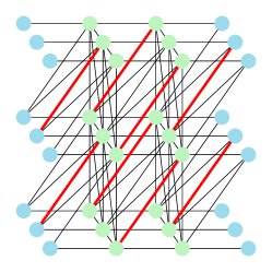
Figure 15: The graph $G_{\textnormal{r}}$ to correct bitflips under circuit-level noise with redundant diagonal boundary edges. The thick red edges are the set of EU edges ‘on a wall’.

Table 2 shows all multiplicity vectors (which for brevity we write sans parentheses and commas) for the graph in Fig. 15. Note the edge orientations shown are for correcting bitflips, so are rotated about the $t$-axis by $\textnormal{}/2$ with respect to those in [37] where the graph used corrects phaseflips, and for which a similar multiplicity table can be computed.

Note also the graph in Fig. 15 has diagonal boundary edges. This is because, merely for bookkeeping, we assign each fault resulting in one defect the orientation of the resultant defect pair had the fault occurred in the bulk of the code. These edges are redundant in the sense that every detector which needs to connect to the boundary is already part of a unique horizontal boundary edge. Mathematically, an edge $e$ is redundant if there already exists another edge $f$ with the same syndrome: $\sigma(\{{e}\})=\sigma(\{{f}\})$.

Error sampling and UF are unaffected by this redundancy, but MWPM and weighted-edge variants of UF only reach their full potential when there are no redundant edges. Therefore, as a final step we merge all redundant edges in $G_{\textnormal{r}}$, resulting in the graph $G$ in Fig. 11(a). To merge an edge $e$ with $f$ we delete $e$ and add the multiplicity vector of $e$ onto that of $f$.

B.3 Other Syndrome Extraction Circuits

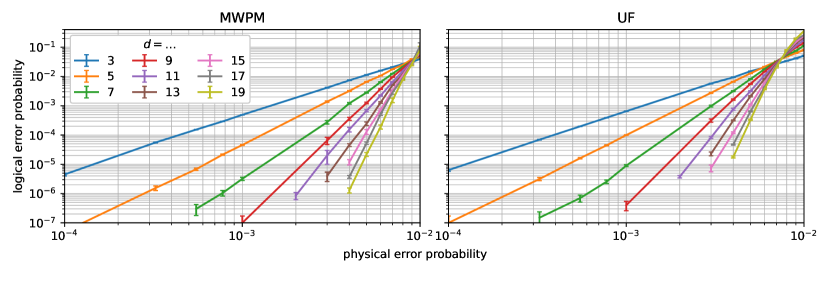
Figure 16: Threshold plots for MWPM and UF under the circuit-level noise model described in Appendix B. Each datapoint is the mean of $1\text{⋅}{10}^{2}3\text{⋅}{10}^{7}$ samples; errorbars show standard error. The threshold of MWPM is $\approx 9.2\text{⋅}{10}^{-3}$.

The circuits in Fig. 14 assume quantum nondemolition measurements (so initialisation is not used) which are native in both Z and X bases. To be more pessimistic about quantum hardware we can consider the following independent restrictions, which both increase the step count of the circuit and affect multiplicity vectors by $\bm{m}\leftarrow\bm{m}+\textnormal{}\bm{m}$ where we specify $\textnormal{}\bm{m}$ below.

• Assuming demolition measurements separates measurement and initialisation. This allows both processes to err independently which increments $m_{4}$ for vertical edges. Also, all data qubits must idle for an extra step which increments $m_{3}$ for horizontal edges. The result is

  $$\textnormal{}\bm{m}^{\textnormal{T}}=\begin{cases*}0010&{S} or {E}\\ 0001&{U}\\ 0000&else,\\ \end{cases*}$$ (19)

  and a step count increase of 1.

• Restricting initialisation (if used) and measurement to, say the Z basis, means X-basis initialisation and measurement each require a Hadamard. This increases the step count of both circuits (if they are performed with equal frequency) by 2, hence adds 2 to $m_{3}$ for horizontal and vertical edges:

  $$\textnormal{}\bm{m}^{\textnormal{T}}=\begin{cases*}0020&{S} or {E} or {U}\\ 0000&else.\end{cases*}$$ (20)

Figure 17 shows syndrome extraction under the combination of these two restrictions.

(a)	(b)

Figure 17: The 8-step syndrome extraction circuit for (a) correcting bitflips; (b) correcting phaseflips.

Note we have slightly optimised the circuit in (a) by initialising and measuring as late and as early as possible, respectively, so the ancilla qubit never suffers from idling faults. Thus for this circuit, Eq. 20 is replaced by

$$\textnormal{}\bm{m}^{\textnormal{T}}=\begin{cases*}0020&{S} or {E}\\ 0000&else.\end{cases*}$$ (21)

For small $\bm{\pi}$, an increase in $\bm{m}$ generally leads to an increase in $\operatorname{pr}(\bm{m},\bm{\pi})$ from Eq. 17 hence a decrease in decoder threshold. Indeed, for UF under the noise model defined by the circuit in (b) we numerically observe a threshold of $\approx 4.5\text{⋅}{10}^{-3}$ (cf. Fig. 1). Generally in this paper, we use the circuits in Fig. 14.

Appendix C Comparison with MWPM

Remark.

While both Helios and our versions of UF grow clusters identically to original UF, their final outputs given the same input $\mathbb{S}$ may not be identical, as $\mathbb{C}$ depends on the choice of the root and spanning tree of each cluster.

It is even possible that, given an error $\mathbb{E}$ which generates $\mathbb{S}$, one of the corrections will cause a logical error while another will not. In other words, the two corrections differ by a logical operation. However, such errors are those where the UF approach itself cannot provide a preference between the two corrections – the choice between them is arbitrary. Indeed, the above scenario necessarily implies a cluster spans between opposite boundaries. Since UF arbitrarily pairs defects within a cluster, any logical difference between corrections within this cluster is random.

One would therefore not expect these differences to lead to any observable difference in decoder accuracy, at least in terms of the subthreshold gradient. This is indeed the case, as Fig. 1 shows.

With this remark, we can unambiguously talk about the accuracy of UF without specifying the particular implementation. Figure 16 shows the accuracy of MWPM and UF for practical noise levels and code distances. We implement MWPM using Sparse Blossom [39] and assign each edge a weight $\ln[(1-p_{e})/p_{e}]$ where $p_{e}$ is its bitflip probability. For both decoders below their respective thresholds, we assume the logical error probability $f$ follows a power law:

$$\frac{f}{f_{\textnormal{th}}}=\Big{(}{\frac{p}{p_{\textnormal{th}}}}\Big{)}^{m}$$ (22)

where $(p,f)_{\textnormal{th}}$ are the coordinates of the threshold. Fig. 18 shows both decoders have the same subthreshold gradient $m(d)$, suggesting their accuracy difference can be characterised solely by their thresholds.

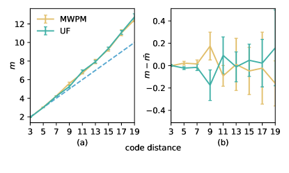
Figure 18: (a) Subthreshold gradient of the lines in Fig. 16 estimated using Weighted Least Squares. The dashed blue line shows the asymptotic ($p\to 0$) value $m=(d+1)/2$ from theory which underestimates the actual value at high distances – a feature already documented for MWPM [40, §5]. (b) Deviation of said gradient from the mean $\bar{m}:=\frac{1}{2}(m_{\text{MWPM}}+m_{\text{UF}})$ of both decoders.

These are around $(0.92,3.8)\cdot$1\text{⋅}{10}^{-2}$$ for MWPM and $(0.75,4.3)\cdot$1\text{⋅}{10}^{-2}$$ for UF, so the former is more accurate.

Recent developments have implemented MWPM with almost-linear mean runtime scaling [39] and parallelisation [41]. One may therefore question the relevance of UF given it is less accurate. However, as UF approximates MWPM [30], any hardware capable of implementing MWPM would likely be able to implement UF and decode faster in the absolute sense. Moreover, and to the best of our knowledge, no one has implemented MWPM in a strictly local fashion. These reasons maintain UF as a competitive decoder, especially in the near term.

References

- [1] Eric Dennis, Alexei Kitaev, Andrew Landahl, and John Preskill. “Topological quantum memory”. Journal of Mathematical Physics 43, 4452–4505 (2002).
- [2] Austin G. Fowler, Matteo Mariantoni, John M. Martinis, and Andrew N. Cleland. “Surface codes: Towards practical large-scale quantum computation”. Physical Review A 86, 032324 (2012).
- [3] Daniel Litinski. “A game of surface codes: Large-scale quantum computing with lattice surgery”. Quantum 3, 128 (2019).
- [4] Jack Edmonds. “Paths, trees, and flowers”. Canadian Journal of Mathematics 17, 449–467 (1965).
- [5] Austin G. Fowler, Adam C. Whiteside, and Lloyd C. L. Hollenberg. “Towards practical classical processing for the surface code”. Physical Review Letters 108, 180501 (2012).
- [6] Guillaume Duclos-Cianci and David Poulin. “Fast decoders for topological quantum codes”. Physical Reviw Letters 104, 050504 (2010).
- [7] Guillaume Duclos-Cianci and David Poulin. “A renormalization group decoding algorithm for topological quantum codes”. In 2010 IEEE Information Theory Workshop. Pages 1–5. (2010).
- [8] James R. Wootton and Daniel Loss. “High threshold error correction for the surface code”. Physical Review Letters 109, 160503 (2012).
- [9] Ben Criger and Imran Ashraf. “Multi-path summation for decoding 2D topological codes”. Quantum 2, 102 (2018).
- [10] Oscar Higgott, Thomas C. Bohdanowicz, Aleksander Kubica, Steven T. Flammia, and Earl T. Campbell. “Improved decoding of circuit noise and fragile boundaries of tailored surface codes”. Physical Review X 13, 031007 (2023).
- [11] Oscar Higgott and Nikolas P. Breuckmann. “Improved single-shot decoding of higher-dimensional hypergraph-product codes”. PRX Quantum 4, 020332 (2023).
- [12] Kao-Yueh Kuo and Ching-Yi Lai. “Exploiting degeneracy in belief propagation decoding of quantum codes”. npj Quantum Information 8, 111 (2022).
- [13] Milap Sheth, Sara Zafar Jafarzadeh, and Vlad Gheorghiu. “Neural ensemble decoding for topological quantum error-correcting codes”. Physical Review A 101, 032338 (2020).
- [14] Ramon W. J. Overwater, Masoud Babaie, and Fabio Sebastiano. “Neural-network decoders for quantum error correction using surface codes: A space exploration of the hardware cost-performance tradeoffs”. IEEE Transactions on Quantum Engineering 3, 1–19 (2022).
- [15] Nicolas Delfosse. “Hierarchical decoding to reduce hardware requirements for quantum computing” (2020). arXiv:2001.11427.
- [16] Kai Meinerz, Chae-Yeun Park, and Simon Trebst. “Scalable neural decoder for topological surface codes”. Physical Review Letters 128, 080505 (2022).
- [17] Gokul Subramanian Ravi, Jonathan M. Baker, Arash Fayyazi, Sophia Fuhui Lin, Ali Javadi-Abhari, Massoud Pedram, and Frederic T. Chong. “Better than worst-case decoding for quantum error correction”. In Proceedings of the 28th ACM International Conference on Architectural Support for Programming Languages and Operating Systems, Volume 2. Pages 88–102. New York, NY, USA (2023). Association for Computing Machinery.
- [18] Samuel C. Smith, Benjamin J. Brown, and Stephen D. Bartlett. “Local predecoder to reduce the bandwidth and latency of quantum error correction”. Physical Review Applied 19, 034050 (2023).
- [19] Nicolas Delfosse and Gilles Zémor. “Linear-time maximum likelihood decoding of surface codes over the quantum erasure channel”. Physical Review Research 2, 033042 (2020).
- [20] Nicolas Delfosse and Naomi H. Nickerson. “Almost-linear time decoding algorithm for topological codes”. Quantum 5, 595 (2021).
- [21] Namitha Liyanage, Yue Wu, Alexander Deters, and Lin Zhong. “Scalable quantum error correction for surface codes using FPGA” (2023). arXiv:2301.08419.
- [22] Alexei Yu Kitaev. “Fault-tolerant quantum computation by anyons”. Annals of Physics 303, 2–30 (2003).
- [23] Tim Chan (2023). code: timchan0/localuf.
- [24] Tim Chan. “Data for ‘Actis: A Strictly Local Union–Find Decoder’” (2023).
- [25] Michael A. Nielsen and Isaac L. Chuang. “Quantum computation and quantum information: 10th anniversary edition”. Cambridge University Press. (2010).
- [26] Xinyu Tan, Fang Zhang, Rui Chao, Yaoyun Shi, and Jianxin Chen. “Scalable surface code decoders with parallelization in time” (2022). arXiv:2209.09219.
- [27] Luka Skoric, Dan E. Browne, Kenton M. Barnes, Neil I. Gillespie, and Earl T. Campbell. “Parallel window decoding enables scalable fault tolerant quantum computation”. Nature Communications 14, 7040 (2023).
- [28] Shui Hu. “Quasilinear time decoding algorithm for topological codes with high error threshold”. Master’s thesis. Delft University of Technology. (2020).
- [29] Oscar Higgott. “PyMatching: A Python package for decoding quantum codes with minimum-weight perfect matching”. ACM Transactions on Quantum Computing 3, 1–16 (2022).
- [30] Yue Wu, Namitha Liyanage, and Lin Zhong. “An interpretation of Union-Find decoder on weighted graphs” (2022). arXiv:2211.03288.
- [31] Robert Endre Tarjan. “Efficiency of a good but not linear set union algorithm”. Journal of the ACM 22, 215–225 (1975).
- [32] Shilin Huang, Michael Newman, and Kenneth R. Brown. “Fault-tolerant weighted union-find decoding on the toric code”. Physical Review A 102, 012419 (2020).
- [33] L. M. K. Vandersypen, H. Bluhm, J. S. Clarke, A. S. Dzurak, R. Ishihara, A. Morello, D. J. Reilly, L. R. Schreiber, and M. Veldhorst. “Interfacing spin qubits in quantum dots and donors—–hot, dense, and coherent”. npj Quantum Information 3, 34 (2017).
- [34] Andrew Richards. “University of Oxford Advanced Research Computing”. (2015).
- [35] Sam J. Griffiths and Dan E. Browne. “Union–find quantum decoding without union–find” (2023). arXiv:2306.09767.
- [36] Ben Barber, Kenton M. Barnes, Tomasz Bialas, Okan Buğdaycı Earl T. Campbell, Neil I. Gillespie, Kauser Johar, Ram Rajan, Adam W. Richardson, Luka Skoric, Canberk Topal, Mark L. Turner, and Abbas B. Ziad. “A real-time, scalable, fast and highly resource efficient decoder for a quantum computer” (2023). arXiv:2309.05558.
- [37] David S. Wang, Austin G. Fowler, and Lloyd C. L. Hollenberg. “Surface code quantum computing with error rates over 1%”. Physical Review A 83, 020302 (2011).
- [38] Emanuel Knill. “Quantum computing with realistically noisy devices”. Nature 434, 39–44 (2005).
- [39] Oscar Higgott and Craig Gidney. “Sparse Blossom: correcting a million errors per core second with minimum-weight matching” (2023). arXiv:2303.15933.
- [40] Austin G. Fowler, Adam C. Whiteside, and Lloyd C. L. Hollenberg. “Towards practical classical processing for the surface code: Timing analysis”. Physical Review A 86, 042313 (2012).
- [41] Yue Wu and Lin Zhong. “Fusion Blossom: Fast MWPM decoders for QEC” (2023). arXiv:2305.08307.