JADES $+$ JEMS: A Detailed Look at the Buildup of Central Stellar Cores and Suppression of Star Formation in Galaxies at Redshifts $3<z<4.5$

Abstract

We present a spatially resolved study of stellar populations in 6 galaxies with stellar masses $M_{*}\sim 10^{10}M_{\sun}$ at $z\sim 3.7$ using 14-filter JWST/NIRCam imaging from the JADES and JEMS surveys. The 6 galaxies are visually selected to have clumpy substructures with distinct colors over rest-frame $3600-4100$ Å, including a bright dominant stellar core that is close to their stellar-light centroids. With 23-filter photometry from HST to JWST, we measure the stellar-population properties of individual structural components via SED fitting using Prospector. We find that the central stellar cores are $\gtrsim 2$ times more massive than the Toomre mass, indicating they may not form via in-situ fragmentation. The stellar cores have stellar ages of $0.4-0.7$ Gyr that are similar to the timescale of clump inward migration due to dynamical friction, suggesting that they likely instead formed through the coalescence of giant stellar clumps. While they have not yet quenched, the 6 galaxies are below the star-forming main sequence by $0.2-0.7$ dex. Within each galaxy, we find that the specific star formation rate is lower in the central stellar core, and the stellar-mass surface density of the core is already similar to quenched galaxies of the same masses and redshifts. Meanwhile, the stellar ages of the cores are either comparable to or younger than the extended, smooth parts of the galaxies. Our findings are consistent with model predictions of the gas-rich compaction scenario for the buildup of galaxies’ central regions at high redshifts. We are likely witnessing the coeval formation of dense central cores, along with the onset of galaxy-wide quenching at $z>3$.

1 Introduction

Over the last two decades, deep imaging surveys with the Hubble Space Telescope (HST), such as GOODS (Giavalisco et al., 2004), CANDELS (Grogin et al., 2011; Koekemoer et al., 2011) and Hubble Frontier Fields (Lotz et al., 2017), have obtained more than $100,000$ rest-frame optical images for mass complete samples of galaxies up to redshift $z=3$. These observations have not only greatly advanced our understanding of galaxies’ structural evolution across cosmic time, but also raised a number of new questions.

It immediately becomes apparent after analyzing those HST images of $1<z<3$ galaxies that they have distinct structural and morphological properties. Relative to galaxies in the local universe, high-redshift galaxies are on average smaller and denser (e.g., Ferguson et al., 2004; van der Wel et al., 2014; Shibuya et al., 2015; Barro et al., 2017), and their morphologies are irregular, and often show large-scale asymmetries and the presence of giant stellar clumps (e.g., Cowie et al., 1995; van den Bergh et al., 1996; Elmegreen & Elmegreen, 2005; Elmegreen et al., 2007; Genzel et al., 2008; Elmegreen et al., 2009; Förster Schreiber et al., 2011; Genzel et al., 2011; Guo et al., 2012, 2015). This latter morphological feature is also present in $z\sim 0$ galaxies, but it has been predominately observed in galaxy mergers (e.g., Conselice et al., 2000; Lotz et al., 2004). By contrast, spatially resolved spectroscopy of high-redshift galaxies shows coherent rotation, suggesting they are more likely to be disks characterized by large velocity dispersion rather than interacting systems (e.g., Förster Schreiber et al., 2006; Genzel et al., 2006; Weiner et al., 2006; Shapiro et al., 2008; Förster Schreiber et al., 2009; Law et al., 2009; Kassin et al., 2012; Simons et al., 2017; Förster Schreiber et al., 2018; Wisnioski et al., 2019; Förster Schreiber & Wuyts, 2020). Understanding this substantial change in galaxies’ structures across cosmic time is the key to constraining models not only of galaxy evolution but also of the interplay between baryonic and dark matter (e.g., Genzel et al., 2020).

Another important process tied to structural transformation is galaxy quenching – the physical processes that control the transition from widespread star formation to quiescence in galaxies. Since $z=3$, star-forming galaxies showed a gradual transformation in their structures from disturbed to normal, smooth disks (Huertas-Company et al., 2015), while the fraction of clumpy star-forming galaxies decreased from $\approx 50\%$ to $\approx 5\%$ (e.g., Murata et al., 2014; Guo et al., 2015). In the meantime, there was a rapid buildup of quiescent galaxies (e.g., Ilbert et al., 2010, 2013; Muzzin et al., 2013; Tomczak et al., 2014) which notably have much larger stellar-mass surface densities than star-forming galaxies of the same masses and redshifts (e.g., Kauffmann et al., 2003; Brinchmann et al., 2004; Franx et al., 2008; Cheung et al., 2012; Mosleh et al., 2017). Is there a causal link between structural transformations and quenching? While a physical link between the two phenomena has been seen in cosmological simulations (Wellons et al., 2015; Zolotov et al., 2015; Tacchella et al., 2016), this question still eludes us observationally, because the structure of galaxies is only known at the time of observation, which makes empirical constraints on the relative timing sequence of the two events difficult (e.g., Bundy et al., 2010; van der Wel et al., 2011; Bruce et al., 2012; Newman et al., 2015; Toft et al., 2017; Newman et al., 2018; Ji & Giavalisco, 2022, 2023).

There is growing evidence that, as they head toward quiescence, galaxies develop a dense stellar core, possibly a bulge (e.g., Kauffmann et al., 2003; Brinchmann et al., 2004; Cheung et al., 2012; Bruce et al., 2014; Lang et al., 2014; Nelson et al., 2014; Williams et al., 2014; Tacchella et al., 2015; Barro et al., 2017; Whitaker et al., 2017; Suess et al., 2021; Dimauro et al., 2022; Ji & Giavalisco, 2023), but the exact physical mechanism responsible for this buildup of central regions remains unknown. While major mergers and weak, non-axisymmetric instabilities (e.g., bars, spiral arms) are believed to drive the development of central structures in $z\sim 0$ disks (Kormendy & Kennicutt, 2004), the physical conditions in high-redshift galaxies are different. First, major mergers are rare and kinematics of the most star-forming galaxies at cosmic noon are instead consistent with a rotating disk. Second, hydrodynamical instabilities are also different in high-redshift disks. This can be understood in a framework of Toomre instability (Toomre, 1964; Binney & Tremaine, 2008), where a rotating gaseous disk becomes unstable when

$$Q=\frac{\sigma\kappa}{\pi G\Sigma}<Q_{c}\sim 1$$ (1)

where $\sigma$ is local gas velocity dispersion, $\kappa$ is epicyclic frequency and $\Sigma$ is local gas surface density. Observations found that star-forming galaxies at cosmic noon are characterized by large $\sigma$, with a typical level of 50 km s^-1 (e.g., Genzel et al., 2008; Förster Schreiber et al., 2009; Genzel et al., 2011) compared to only a few km s^-1 observed for nearby spiral galaxies. In addition, high-redshift galaxies have higher gas fractions, with a typical value of $\approx 50\%$ compared to a few to 10% at $z\sim 0$ (Tacconi et al., 2020). With these properties, high-redshift disks have $Q\sim 1$ (i.e., the entire disk is unstable/marginally stable), while low-redshift disks are largely stable with $Q>1$. These lead to two direct consequences in high-redshift galaxies. First, high-redshift disks are subject to violent gravitational instabilities that lead to the formation of giant stellar clumps. Second, the timescale for the inward migration of clumps toward the gravitational center is much shorter at high redshifts than in the nearby universe (Dekel et al., 2009; Genzel et al., 2011).

A popular hypothesis is thus that massive stellar cores in high-redshift galaxies are the result of unstable, gas-rich disks, which first fragment into giant stellar clumps that then rapidly migrate inward and finally coalesce to form dense stellar cores (e.g., Noguchi, 1999; Immeli et al., 2004; Bournaud et al., 2007; Elmegreen et al., 2008; Dekel et al., 2009; Ceverino et al., 2010; Bournaud et al., 2014). On the one hand, the observed radial color gradients of star-forming clumps seem to support this hypothesis (Förster Schreiber et al., 2011; Guo et al., 2012, 2015; Shibuya et al., 2016; Soto et al., 2017; Mandelker et al., 2017). On the other, studies of gas kinematics find evidence that strong outflows can launch from the clump sites (Genzel et al., 2011), arguing that clumps might be self-disrupted by strong stellar feedback which can significantly reduce the growth rate of central stellar cores (Murray et al., 2010; Genel et al., 2012; Hopkins et al., 2012; Buck et al., 2017). Thus, it remains unknown to what extent violent disk instabilities drive the growth of central regions in high-redshift galaxies.

The James Webb Space Telescope (JWST; Gardner et al., 2023) is revolutionary for studying the detailed physics of structural transformations and quenching at cosmic noon. For the first time, we can get images at rest-frame optical and NIR wavelengths, with a sensitivity that is not attainable with HST, for galaxies beyond $z>3$, closer to the time of early core/bulge formation and quenching. This guarantees more direct constraints on the underlying physics. With sub-kpc spatial resolution, JWST’s Near Infrared Camera (NIRCam, Rieke et al. 2023) can resolve a physical scale comparable to the typical Toomre length of gaseous disks at cosmic noon (e.g., Elmegreen et al., 2009; Escala & Larson, 2008; Dekel et al., 2009; Genzel et al., 2011), promising to identify individual stellar substructures. Together with the ancillary HST data, imaging that covers truly panchromatic swathes from rest-frame UV through NIR enable us to put unprecedented constraints on the detailed, spatially resolved mass assembly history of galaxies at high redshifts.

In this paper, we present the spatially resolved stellar populations in 6 galaxies at $3<z<4.5$. This redshift range represents one of the key epochs of the universe when quenching becomes a significant process (Muzzin et al., 2013; Schreiber et al., 2018; Merlin et al., 2019; Shahidi et al., 2020; Carnall et al., 2023a, b), which can provide unique insight into the role that substructures among massive galaxies may play in the transition from star-forming disks to bulge-dominated quiescent objects. The galaxies are visually selected to have bright and red central regions. We show that these galaxies are very likely in the act of developing their stellar cores/bulges. We discuss their implications on structural transformations and quenching at cosmic noon. Throughout this paper, we adopt the $\Lambda$CDM cosmology with Planck Collaboration et al. 2020 parameters, i.e., $\Omega_{m}=0.315$ and $\rm{h=H_{0}/(100km\,s^{-1}\,Mpc^{-1})=0.673}$.

2 Observations & Analysis

2.1 Sample Selection

Table 1: Physical Properties of the Final Sample Presented in this Work.

ID	RA	DEC	Redshift	Redshift Ref. (a)	log M∗ (b)	SFR (b)	Stellar Age (b),(c)
	(Deg)	(Deg)			(M☉)	(M☉ yr-1)	(Gyr)
JADES-JEMS-13396	53.14921	-27.79158	3.559	MUSE	10.00 ${}^{+0.02}_{-0.04}$	13.5 ${}^{+0.8}_{-0.6}$	0.8 ${}^{+0.1}_{-0.1}$
JADES-JEMS-15157	53.13943	-27.78009	3.591	MUSE & FRESCO (d)	9.36 ${}^{+0.09}_{-0.11}$	1.3 ${}^{+1.0}_{-0.4}$	0.4 ${}^{+0.2}_{-0.1}$
JADES-JEMS-6885	53.12832	-27.84573	3.698	FRESCO	9.87 ${}^{+0.03}_{-0.07}$	7.4 ${}^{+1.1}_{-0.9}$	0.4 ${}^{+0.2}_{-0.2}$
JADES-JEMS-16296	53.15651	-27.77227	3.53	Photometric	9.65 ${}^{+0.05}_{-0.06}$	5.4 ${}^{+1.2}_{-0.9}$	0.5 ${}^{+0.3}_{-0.2}$
JADES-JEMS-14436	53.13306	-27.78456	3.67	Photometric	10.34 ${}^{+0.07}_{-0.09}$	11.8 ${}^{+2.5}_{-1.9}$	0.8 ${}^{+0.1}_{-0.1}$
JADES-JEMS-11059	53.13484	-27.80887	4.07	Photometric	9.59 ${}^{+0.08}_{-0.07}$	9.6 ${}^{+0.7}_{-0.6}$	0.4 ${}^{+0.1}_{-0.2}$

• (a) Redshifts are from either the MUSE/HUDF Data Release 2 (Bacon et al., 2022), or [SIII]$\lambda$9531 emission line detected in the NIRCam WFSS spectra (Sun, F. private communication) obtained by the FRESCO survey (Oesch et al., 2023), or photometric redshifts when spectroscopic ones are not available. (b) Reported values are from the Prospector SED fitting with our fiducial model (Section 2.4). (c) Mass-weighted stellar age. (d) The redshift of this galaxy derived using the [SIII]$\lambda$9531 in its FRESCO spectrum is sightly different from using the Ly$\alpha$ in its MUSE spectrum, with the former being 3.591 and latter being 3.605.

The galaxies presented in this paper are drawn from an initial sample of HST/F160W-selected galaxies with $3<z<4.5$ from the latest CANDELS/GOODS-S catalog obtained by the ASTRODEEP project (Merlin et al., 2021). By selection, we first retain 361 galaxies in the footprint of the JWST Extragalactic Medium-band Survey (JEMS) ($\approx 10$ arcmin², Williams et al., 2023, JWST Cycle 1, PID: 1963), which also appear in the footprint of the JWST Advanced Deep Extragalactic Survey (JADES, Eisenstein et al. 2017), a collaborative program between the NIRCam and NIRSpec GTO teams. These yield a total of 14-filter NIRCam imaging at $\lambda\approx 0.8-5\micron$ (Section 2.2). Together with the ancillary data from HST, this high angular resolution imaging data across a total of 23 filters enables us to perform detailed stellar-population analysis in these galaxies. With the new photometry from NIRCam imaging (Section 2.2), we then run SED fitting with the code Prospector (Johnson et al., 2021) using the fiducial model described in Section 2.4, during which we set redshift as a free parameter. Finally, we only retain 301 galaxies as the parent sample whose best-fit redshifts from our new SED fitting are still in the range of $3<z_{\rm{phot}}<4.5$.

For each one of the galaxies in the parent sample, we visually check the color maps produced by its NIRCam F150W, F182M and F210M images, which probe rest-frame light at $\sim$ 3000, 4000 and 4500 Å, respectively. This wavelength range, i.e. around the 4000 Å break, is chosen because it contains key information about stellar-population properties, especially stellar ages (e.g., Bruzual A., 1983; Kauffmann et al., 2003). Our visual identification finds 37 (out of 301) galaxies having substructures with distinct F150W/F182M/F210M colors. As Figure 1 shows, these 37 galaxies are at the massive end of our JEMS parent sample, i.e. the majority of them have stellar masses $>10^{9}M_{\sun}$, which is expected because the visual selection is biased toward bright substructures in relatively bright galaxies. Among 36 galaxies in the parent sample with masses $>10^{9.5}M_{\sun}$, 22 of them are visually identified to have substructures, corresponding to a fraction of $61\pm 17\%$. Interestingly, at face value this fraction is in quantitative agreement with earlier HST studies of the fraction of galaxies with UV clumps at slightly lower redshifts $2.5<z<3$ (e.g., Shibuya et al., 2016; Sattari et al., 2023). While we caution that the methods used to identify clumps can significantly affect the results, we defer more detailed investigation of this impact to a future work with larger samples and more uniform selection methods.

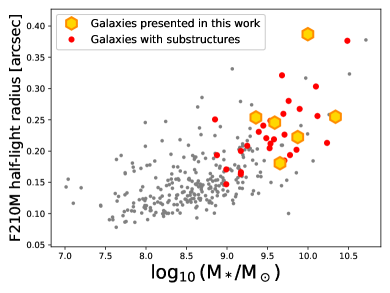
Figure 1: The parent sample of $3<z<4.5$ galaxies from JEMS. The $x$-axis shows the stellar mass from our Prospector SED fitting (Section 2.4), the $y$-axis shows the half-light radius derived directly from the F210M surface brightness profile (no PSF-convolved analysis included). Red circles show the 37 galaxies with visually identified substructures having distinct rest-frame colors at 4000 Å. The golden hexagons show the final sample of 6 galaxies with red, massive cores presented in this work (see Section 2.1 for the detailed sample selection).

Our analysis finds that the 37 galaxies with visually identified substructures have diverse spatially resolved stellar populations, representing different stages of galaxy structural transformations. This motivates this and upcoming papers in this series, where we address different physical mechanisms associated with those different stages of structural transformations. In this first paper, we only focus on a group of 6 galaxies whose basic information is present in Table 1. Figure 2 and 3 show their 23-filter cutouts.

In each one of the 6 galaxies, there is a bright and red (at rest-frame $\sim$ 4000 Å) clumpy substructure, which we refer to as C1. C1 is always close to the center of stellar-light distribution, accompanied by additional off-center, minor clumpy substructures (named as C2 and C3, if present). Our analysis below shows that C1 is more massive than what one would expect from a single collapse due to the Toomre instability, and has a star formation history (SFH) that shows a recent major star-formation episode started $\sim 0.5-1$ Gyr ago that peaked at $\sim 0.1-0.3$ Gyr prior to the time of observation. The formation of the stellar core C1 and its impact, if any, on star formation will be the main focus of this paper.

2.2 Observations & Data Reduction

The 6 galaxies have been observed with deep imaging in 14 JWST/NIRCam filters. These include 9-filter images (F090W, F115W, F150W, F200W, F277W, F335M, F356W, F410M, F444W) acquired as part in the GOODS-S portion of JADES, and 5 additional medium-filter images (F182M, F210M, F430M, F460M and F480M) acquired by JEMS.

The NIRCam observations of all 14 filters are reduced using a consistent method, which has been briefly summarized in Robertson et al. (2022) and will be presented in detail in Rieke et al. (2023 in preparation) and Tacchella et al. (2023 in preparation). In short, we process the raw images with the JWST Calibration Pipeline v1.8.1 with the CRDS pipeline mapping (pmap) context 1009. To perform the detector-level corrections and obtain count-rate images, we run the Stage 1 of the JWST pipeline with default parameters, during which we also mask and correct for the “snowballs” effect caused by charge deposition arising from cosmic ray hits. We then run the Stage 2 of the JWST pipeline, with default parameters, to perform the flat-fielding and flux calibration, after which we perform several custom corrections including the removal of $1/f$ noise and the subtraction of 2D background from the images, and the correction for the “wisp” features in the short-wavelength (SW, i.e. filters bluer than F277W) images. Afterwards, for individual exposures of a given visit, we match sources to the World Coordinate System of a reference catalog constructed from HST F160W mosaics in the GOODS-S field with astrometry tied to Gaia-EDR3 (Gaia Collaboration et al., 2021), calculate astrometric corrections and then run the Stage 3 of the JWST pipeline to combine together all those individual exposures. Finally, we combine individual visit-level mosaics together to create the final mosaic, where we choose a pixel scale of 0.03 arcsec pixel^-1 for all filters.

The ancillary HST data used in this work are taken from the latest Hubble Legacy Fields Data Release in the GOODS-S field (Illingworth et al., 2016; Whitaker et al., 2019), including the imaging data of the ACS/WFC F435W, F606W, F775W, F850LP and F814W filters, and of the WFC3 F105W, F125W, F140W and F160W filters. For all those HST images, we have (1) tied them to the same astrometry and (2) resampled them to the same pixel scale as those of our NIRCam images (Robertson et al 2023 in preparation).

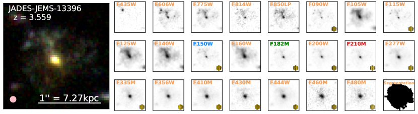
(a) JADES–JEMS–13396

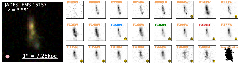
(b) JADES–JEMS–15157

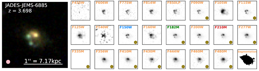
(c) JADES–JEMS–6885

Figure 2: Panchromatic HST and JWST/NIRCam images of the three galaxies with spectroscopically confirmed redshifts $z_{\rm{spec}}$. The RGB image shown on the left is made with JWST/NIRCam F150W (B), F182M (G) and F210M (R) images. The pink circle at the bottom-left marks the FWHM of the NIRCam/F210M PSF (Appendix A). Small panels show cutouts of individual 23 filters covering observed $\lambda\approx 0.35-5\micron$ included in the analysis of this work, where the newly obtained 14-filter NIRCam images are labelled with a hexagon symbol at the bottom-right. The last small panel shows the segmentation map. All cutouts are shown in a linear color scale. We adjust the pixel value range of each cutout to highlight the substructures.

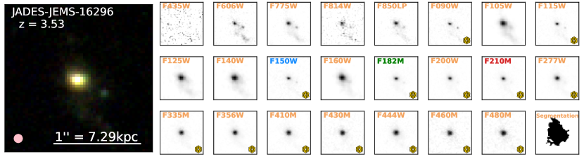
(a) JADES–JEMS–16296

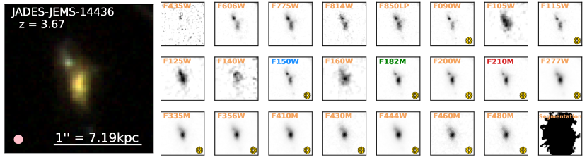
(b) JADES–JEMS–14436

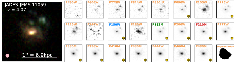
(c) JADES–JEMS–11059

Figure 3: Similar to Figure 2, but for the remaining three galaxies with photometric redshifts $z_{\rm{phot}}$.

2.3 Photometry

For each galaxy, we perform aperture-matched photometry for (1) integrated flux, (2) individual substructures and (3) a smooth component. The integrated flux is defined as total flux in the pixel aperture generated from a galaxy’s segmentation map generated by JADES (Robertson et al., 2022). For fluxes of individual substructures, we use customized elliptical apertures which are illustrated in the RGB images in Figure 5 and 6. Finally, the smooth component is defined as integrated flux minus co-added fluxes of individual substructures.

Point Spread Functions (PSFs) of all images are first homogenised to that of NIRCam/F444W. To do so, in the footprint of JEMS, we visually identify 13 isolated, bright stars which are unsaturated across all filters from HST through JWST. We then build effective PSFs (ePSFs) following the method from Anderson & King (2000). For NIRCam filters, we have also generated model PSFs (mPSFs) using the package Webbpsf(v1.1.1, Perrin et al., 2012, 2014), during which we also took into account the observational (e.g., source location on detectors, optical path difference) and data reduction (e.g., mosaicking) effects. As shown in Appendix A, we find excellent agreement between ePSFs and mPSFs, with a typical difference of $\lesssim 1\%$. We then homogenise ePSFs using the package Pypher which calculates the convolution kernel based on Wiener filtering with a regularisation factor (Boucaud et al., 2016). Finally, we perform aperture-matched photometry in the PSF-matched images.

To estimate photometric uncertainties, we follow Labbé et al. (2005) to first use randomly placed apertures in empty (i.e., no sources) regions in the images to estimate the growth of noise as a function of the linear size of aperture. We then fit the function using the parametrization of Quadri et al. (2007) and finally estimate photometric uncertainties using equation 5 in Whitaker et al. (2011). This procedure will be presented in detail in Robertson et al. (2023 in preparation).

2.4 Measuring Stellar-population Properties

We model panchromatic Spectral Energy Distributions (SEDs) to derive stellar-population properties of individual structural components, with the emphasis on robustly measuring their stellar masses, ages and SFHs. For each one of the galaxies, we perform two rounds of SED fitting. The first round aims at checking the physical association of all structural components, as opposed to the case when sources at different distances are projected onto the regions of sky in close proximity of each other. During the SED fitting of this round, we set redshift as a free parameter with a flat prior of $z\in(0,10)$. We then check posterior distributions of redshift, and consider structural components as being physically linked when the difference in the median of their redshift posteriors is $\leq 0.1$. Afterwards, we fix redshifts of all components to either the spectroscopic redshift if available or the best-fit value that we derive from the first-round SED fitting using the galaxy’s integrated photometry, and run the second-round SED fitting. The fitting results are shown in Figure 5 and 6, and will be discussed in Section 3.1. Below, we detail the model assumptions of our SED fitting.

2.4.1 Basic setup of the Prospector fitting

The SED fitting code Prospector (Johnson et al., 2021) is elected to use in this work. It is built upon a fully Bayesian framework that makes it possible to fit galaxies’ SEDs with complex models of stellar population synthesis.

Regarding the basic setup of Prospector fitting, we adopt the Flexible Stellar Population Synthesis (FSPS) code (Conroy et al., 2009; Conroy & Gunn, 2010) where we use the stellar isochrone libraries MIST (Choi et al., 2016; Dotter, 2016) and the stellar spectral libraries MILES (Falcón-Barroso et al., 2011). During the modeling, we use the MCMC sampling code dynesty (Speagle, 2020) which adopts the nested sampling procedure (Skilling, 2004). We assume the Kroupa 2001 initial mass function (IMF) for consistency with the IMF used in the Byler et al. (2017) nebular continuum and line emission model which we adopt in our SED modeling. We adopt the Madau (1995) IGM absorption model.

We set the stellar metallicity as a free parameter and assume a flat prior in logarithmic space $\log(Z_{*}/Z_{\sun})\in(-2,0.19)$, where $Z_{\sun}=0.0142$ is solar metallicity. The upper limit of the prior is chosen because it is the highest metallicity that the MILES library has. We also leave the gas-phase metallicity $Z_{\rm{gas}}$ and ionization parameter $U$ as free parameters during the fitting, where we use flat priors of $\log(Z_{\rm{gas}}/Z_{\sun})\in(-2,0.5)$ and $\log U\in(-4,1)$.

Following Tacchella et al. (2022a), we assume a two-component dust attenuation model where the dust attenuation of nebular emission and young stellar populations, and of old stellar populations, are treated differently (Charlot & Fall, 2000). For stellar populations older than 10 Myr, we assume the dust attenuation using the parametrization from Noll et al. (2009), i.e.,

$$\tau_{\rm{dust,2}}(\lambda)=\frac{\hat{\tau}_{\rm{dust,2}}}{4.05}(k^{{}^{\prime}}(\lambda)+D(\lambda))\left(\frac{\lambda}{5500\rm{\AA}}\right)^{\delta}$$ (2)

where $\rm{\hat{\tau}_{dust,2}}$ and $\delta$ correspond to dust2 and dust_index in the FSPS, $k^{{}^{\prime}}(\lambda)$ is the Calzetti et al. (2000) dust attenuation law and $D(\lambda)$ is the Lorentzian-like profile used to describe the UV dust bump at 2175 Å. Instead of setting $D(\lambda)$ as a free parameter, we tie it to $\delta$ following the results of Kriek & Conroy (2013). Therefore, the dust attenuation for the older stellar populations only has two free parameters, $\delta$ and $\rm{\hat{\tau}_{dust,2}}$. We assume flat priors for both parameters, i.e., $\delta\in(-1,0.4)$ and $\rm{\hat{\tau}_{dust,2}}\in(0,10)$. For stellar populations younger than 10 Myr, we assume the same dust attenuation law as for the nebular emission, which has a functional form of

$$\tau_{\rm{dust,1}}(\lambda)=\hat{\tau}_{\rm{dust,1}}\left(\frac{\lambda}{5500\rm{\AA}}\right)^{-1},$$ (3)

where $\rm{\hat{\tau}_{dust,1}}$ corresponds to the parameter dust1 in the FSPS. Instead of modeling $\rm{\hat{\tau}_{dust,1}}$ as an independent free parameter, we tie it to $\rm{\hat{\tau}_{dust,2}}$ and model their ratio using a clipped normal prior centered at 1, with a width of 0.3 and in the range of $\rm{\hat{\tau}_{dust,1}}/\rm{\hat{\tau}_{dust,2}}\in(0,2)$.

We also include AGN dust torus templates from Nenkova et al. (2008a) and Nenkova et al. (2008b), but we stress that the purpose of including this AGN component is not to quantitatively constrain the AGN strength, since the data coverage we currently have does not have power to do so. Instead, the purpose simply is to marginalize over it in order to check how the AGN component can affect the fitting results. This adds two free parameters: the ratio of bolometric luminosity from the galaxy divided by that from the AGN ($f_{\rm{AGN}}$), and the optical depth of clumps in AGN dust torus at 5500 Å ($\tau_{\rm{AGN}}$). We assume flat priors in logarithmic space for both parameters, i.e., $f_{\rm{AGN}}\in(10^{-5},3)$ and $\tau_{\rm{AGN}}\in(5,150)$. We find that $f_{\rm{AGN}}$ is consistent with zero for all sample galaxies, which is in line with the fact that these galaxies are not classified as AGN using other different selection methods, including X-ray (Luo et al., 2017), IRAC colors (Ji et al., 2022) and multi-wavelength selections (Lyu et al., 2022).

2.4.2 Reconstructing star formation histories

One key feature of Prospector is that it allows flexible parameterizations of galaxies’ SFHs, both in parametric and nonparametric forms. This has been demonstrated as crucial to reducing systematic biases in the measurements of stellar mass, star formation rate and stellar age (Leja et al., 2019). Several recent studies have further shown that statistically, Prospector is capable of reconstructing high-fidelity nonparametric SFHs for synthetic galaxies generated from cosmological simulations (Leja et al., 2019; Johnson et al., 2021; Tacchella et al., 2022a; Ji & Giavalisco, 2022).

For the fiducial SFH, we assume a piece-wise, nonparametric form composed of $N_{\rm{SFH}}=9$ lookback time bins ($t_{\rm{lookback}}$, i.e., the time prior to the time of observation), where star formation rate is constant in each bin. Among the 9 lookback time bins, the first two bins are fixed to be $0-30$ and $30-100$ Myr in order to capture the recent star formation activity; the last bin is assumed to be $\rm{0.85t_{H}-t_{H}}$ where $\rm{t_{H}}$ is the Hubble Time at the time of observation; and the remaining 6 bins are evenly spaced in logarithmic space between $\rm{100\,Myr-0.85t_{H}}$. As have been extensively tested by Leja et al. (2019) using mock observations of simulated galaxies (see their Figure 15), the recovered physical properties are largely insensitive to $N_{\rm{SFH}}$ when it is greater than 5. This is also found later through our analysis presented in Section 3.1 and Figure 4.

The procedure above to reconstruct nonparametric SFHs potentially suffers from overfitting problems, because it includes “more bins than the data warrant” (Leja et al., 2019). An effective solution to mitigate the issue is to choose a prior weight for physically plausible forms, as opposed to letting the SFHs have a fully arbitrary shape (Carnall et al., 2019a; Leja et al., 2019). Our fiducial measures use the continuity prior that has been demonstrated to work well across various galaxy types (Leja et al., 2019). Recent studies have noted the systematics introduced by assumed priors to reconstructed SFHs (Tacchella et al., 2022b; Ji & Giavalisco, 2022; Suess et al., 2022). To check possible systematics in our measurements, we therefore also experiment using another well-tested Dirichlet prior (Leja et al., 2017). In addition, we have also tested our results using the parametric delayed-tau model. As we show in Appendix B, the results of this work remain qualitatively unchanged using these different methods of SFH reconstructions. In the remainder of main text, our discussion thus will only focus on measurements from the continuity prior.

2.5 Measuring Morphological Properties of the Substructures

To estimate intrinsic stellar masses (Section 3.2) and stellar-mass surface densities (Section 4.2) of the clumpy substructures, we perform PSF-convolved morphological fitting. For each one of the galaxies, we simultaneously model the 2D light distributions of all clumpy substructures with the fitting code forcepho (Johnson et al. 2023 in preparation), which adopts a fully MCMC framework and performs the fitting on the basis of individual NIRCam exposures, as opposed to performing the fitting in a drizzled image (i.e., a mosaic). In this way, parameter uncertainties are better estimated because correlations of adjacent image pixels, and, more importantly here given the complex morphologies of the galaxies, correlations of fluxes from neighbouring substructures are naturally taken into account (see Robertson et al. 2022 and Tacchella et al. 2023 for a brief discussion). A redder NIRCam filter generally better probes the stellar-mass distribution. Meanwhile, a better angular resolution also helps to better separate fluxes from individual substructures. As Figures 2 and 3 show, it becomes increasingly difficult to separate individual substructures in images of longer-wavelength filters owing to their worse angular resolutions compared to shorter wavelengths. We thus perform the forcepho analysis using the reddest NIRCam’s SW filter we have, i.e., F210M which probes rest-frame $\sim$ 5000Å of the six galaxies. Finally, we model each clumpy substructure using a single Sérsic profile.

Figure 7 shows results of the forcepho fitting. As the residual map shows, each one of the substructures is well fit by a single Sérsic profile. The $\chi$ map also confirms the presence of the Smooth component surrounding the clumpy substructures in each one of the galaxies. Ideally, in the forcepho fitting we could add an additional morphological component to model this Smooth component together with the clumpy substructures. However, we find that a single Sérsic profile is unable to describe the Smooth component, because its morphology is rather complex with large-scale asymmetries. In principle, we could assume a more complex model for it, e.g., a summation of several Sérsic profiles. But such a model is purely arbitrary and it would be hard to understand and control the systematic errors behind it. We therefore decide not to model the Smooth component in the forcepho fitting. One concern is then how this can affect the morphological fits to the clumpy substructures. While it can be significant for faint clumps C2 and C3, we argue that the effect should be minor for C1 (which is the focus of this work) because the ratio of the median residual flux (primarily from the Smooth component) to the peak flux of C1 is only $\sim 0.1-4\%$.

3 Results

In this Section, we present the spatially resolved stellar populations of the 6 galaxies. In particular, we focus on the properties of the red, massive core C1 in each one of the galaxies, and discuss the constraints on its formation mechanisms.

Table 2: Properties of Spatially Resolved Stellar Populations

ID	Redshift	Component	F${}_{\nu}^{\rm{F150W}}$ (a)	log M∗ (b)	SFR (b),(c)	Stellar Age (b)	sSFR (b)
			(nJy)	(M☉)	(M☉ yr-1)	(Gyr)	(Gyr-1)
JADES-JEMS-13396	3.559	C1	24.6 $\pm$0.8	9.40 ${}^{+0.03}_{-0.04}$	2.7 ${}^{+0.2}_{-0.3}$	0.7 ${}^{+0.1}_{-0.2}$	1.07 ${}^{+0.10}_{-0.15}$
		Smooth	212.8 $\pm$11.4	9.88 ${}^{+0.06}_{-0.13}$	13.4 ${}^{+2.3}_{-1.6}$	0.6 ${}^{+0.1}_{-0.2}$	1.76 ${}^{+0.38}_{-0.56}$
		Integrated	237.4 $\pm$11.7	10.00 ${}^{+0.02}_{-0.04}$	13.5 ${}^{+0.8}_{-0.6}$	0.8 ${}^{+0.1}_{-0.1}$	1.35 ${}^{+0.10}_{-0.13}$
JADES-JEMS-15157	3.591	C1	11.4 $\pm$0.7	8.71 ${}^{+0.10}_{-0.08}$	0.2 ${}^{+0.1}_{-0.1}$	0.6 ${}^{+0.1}_{-0.2}$	0.38 ${}^{+0.21}_{-0.20}$
		C2	9.2 $\pm$0.9	8.02 ${}^{+0.15}_{-0.43}$	0.3 ${}^{+0.1}_{-0.1}$	0.5 ${}^{+0.1}_{-0.4}$	2.86 ${}^{+1.37}_{-2.99}$
		C3	9.8 $\pm$0.8	8.55 ${}^{+0.09}_{-0.15}$	0.2 ${}^{+0.1}_{-0.1}$	0.5 ${}^{+0.1}_{-0.3}$	0.56 ${}^{+0.30}_{-0.34}$
		Smooth	58.7 $\pm$7.3	9.35 ${}^{+0.07}_{-0.05}$	0.4 ${}^{+0.4}_{-0.2}$	0.7 ${}^{+0.1}_{-0.2}$	0.17 ${}^{+0.18}_{-0.09}$
		Integrated	89.2 $\pm$8.3	9.36 ${}^{+0.09}_{-0.11}$	1.3 ${}^{+1.0}_{-0.4}$	0.4 ${}^{+0.2}_{-0.1}$	0.56 ${}^{+0.45}_{-0.22}$
JADES-JEMS-6885	3.698	C1	39.9 $\pm$1.6	9.19 ${}^{+0.07}_{-0.03}$	1.5 ${}^{+0.1}_{-0.2}$	0.6 ${}^{+0.1}_{-0.1}$	0.96 ${}^{+0.16}_{-0.14}$
		C2	16.8 $\pm$0.8	8.30 ${}^{+0.10}_{-0.15}$	1.2 ${}^{+0.1}_{-0.1}$	0.3 ${}^{+0.1}_{-0.1}$	6.01 ${}^{+1.47}_{-2.13}$
		C3	12.2 $\pm$0.8	8.13 ${}^{+0.08}_{-0.09}$	1.2 ${}^{+0.1}_{-0.2}$	0.1 ${}^{+0.1}_{-0.1}$	8.89 ${}^{+1.79}_{-2.36}$
		Smooth	169.0 $\pm$13.0	9.62 ${}^{+0.07}_{-0.21}$	3.6 ${}^{+1.1}_{-0.6}$	0.4 ${}^{+0.2}_{-0.2}$	0.86 ${}^{+0.29}_{-0.14}$
		Integrated	238.1 $\pm$14.0	9.87 ${}^{+0.03}_{-0.07}$	7.4 ${}^{+1.1}_{-0.9}$	0.4 ${}^{+0.2}_{-0.2}$	0.99 ${}^{+0.16}_{-0.20}$
JADES-JEMS-16296	3.53	C1	42.5 $\pm$1.3	8.82 ${}^{+0.02}_{-0.03}$	2.7 ${}^{+0.1}_{-0.1}$	0.5 ${}^{+0.1}_{-0.1}$	4.08 ${}^{+0.24}_{-0.32}$
		C2	7.1 $\pm$0.9	7.88 ${}^{+0.05}_{-0.08}$	0.4 ${}^{+0.1}_{-0.1}$	0.1 ${}^{+0.1}_{-0.1}$	5.27 ${}^{+1.45}_{-1.63}$
		Smooth	80.8 $\pm$7.3	9.37 ${}^{+0.02}_{-0.01}$	0.9 ${}^{+0.1}_{-0.2}$	0.9 ${}^{+0.1}_{-0.1}$	0.38 ${}^{+0.04}_{-0.08}$
		Integrated	130.6 $\pm$8.4	9.65 ${}^{+0.05}_{-0.06}$	5.4 ${}^{+1.2}_{-0.9}$	0.5 ${}^{+0.3}_{-0.2}$	1.20 ${}^{+0.30}_{-0.26}$
JADES-JEMS-14436	3.67	C1	87.8 $\pm$1.8	9.58 ${}^{+0.05}_{-0.02}$	3.9 ${}^{+0.2}_{-0.2}$	0.4 ${}^{+0.1}_{-0.1}$	1.02 ${}^{+0.12}_{-0.07}$
		C2	38.5 $\pm$0.9	9.32 ${}^{+0.11}_{-0.06}$	5.8 ${}^{+0.6}_{-0.7}$	0.3 ${}^{+0.2}_{-0.1}$	2.77 ${}^{+0.75}_{-0.50}$
		Smooth	169.9 $\pm$17.0	10.05 ${}^{+0.04}_{-0.06}$	2.8 ${}^{+0.6}_{-0.6}$	0.9 ${}^{+0.1}_{-0.2}$	0.24 ${}^{+0.05}_{-0.06}$
		Integrated	296.3 $\pm$18.0	10.34 ${}^{+0.07}_{-0.09}$	11.8 ${}^{+2.5}_{-1.9}$	0.8 ${}^{+0.1}_{-0.1}$	0.53 ${}^{+0.14}_{-0.14}$
JADES-JEMS-11059	4.07	C1	47.8 $\pm$1.2	9.32 ${}^{+0.02}_{-0.03}$	2.0 ${}^{+0.1}_{-0.1}$	0.7 ${}^{+0.1}_{-0.1}$	0.95 ${}^{+0.06}_{-0.08}$
		C2	24.0 $\pm$1.1	7.97 ${}^{+0.05}_{-0.07}$	1.2 ${}^{+0.1}_{-0.1}$	0.4 ${}^{+0.1}_{-0.1}$	12.85 ${}^{+1.82}_{-2.33}$
		C3	8.2 $\pm$0.5	8.22 ${}^{+0.22}_{-0.39}$	0.4 ${}^{+0.1}_{-0.1}$	0.5 ${}^{+0.1}_{-0.3}$	2.41 ${}^{+1.36}_{-2.24}$
		Smooth	164.0 $\pm$11.6	9.81 ${}^{+0.07}_{-0.12}$	7.3 ${}^{+1.7}_{-2.5}$	0.3 ${}^{+0.4}_{-0.2}$	1.13 ${}^{+0.32}_{-0.49}$
		Integrated	244.2 $\pm$12.9	9.59 ${}^{+0.08}_{-0.07}$	9.6 ${}^{+0.7}_{-0.6}$	0.4 ${}^{+0.1}_{-0.2}$	2.46 ${}^{+0.48}_{-0.42}$

• (a) Fluxes from aperture photometry in PSF-matched NIRCam/F150W images. (b) Reported values are from the Prospector SED fitting with our fiducial model (Section 2.4). (c) Instantaneous SFR from SED fitting, i.e., SFR in the first lookback time bin (30 Myr) of a nonparametric SFH.

3.1 Spatially Resolved Stellar Populations

Table 2 presents the physical properties derived from the fiducial Prospector model described in Section 2.4. To check the SED fitting results, we first compare the stellar mass and star formation rate derived using the integrated flux with the sum of that measured for individual components, i.e., substructures plus the Smooth component. We note that these two values are not necessarily consistent with each other, because summation of the measurements of $N$ individual components is equivalent to fitting a galaxy’s SED with $(N-1)$ $\times$ more free parameters than using its integrated flux alone. Yet, excellent agreement between the two measurements is seen in Figure 4, showing the consistency and robustness of our SED fitting.

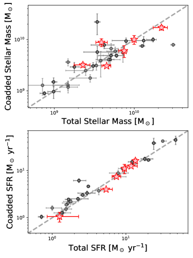
Figure 4: Comparisons of the stellar-mass (top panel) and star formation rate (bottom panel) measures. The $x$-axis shows the measure using integrated flux, and the $y$-axis shows the results by coadding the measures of individual structural components (i.e. substructures+smooth) together. In the figure we plot all 37 galaxies showing distinct substructures around the rest-frame 4000 Å (Section 2.1), and the final sample of 6 galaxies presented in this paper are marked with the red star symbols. We see excellent agreement between the two measurements.

Figure 5 and 6 show the spatially resolved SED fitting results in detail. The SED shapes of individual structural components differ across the entire rest-frame UV to NIR wavelengths, suggesting that stellar populations vary significantly within each one of the galaxies. This highlights the importance of having spatially resolved measures of stellar populations to get a comprehensive view on the mass assembly processes in high-redshift galaxies. We refer the readers to Appendix C for detailed descriptions of SED fitting results of individual galaxies. In the list below, we only summarize the key findings. In each one of the galaxies,

• the red stellar core C1 is the dominant, most massive one among all identified clumpy substructures. Relative to the off-center, minor clumps C2 and C3, C1 contains older stellar populations, spanning a range in mass-weighted stellar age of $0.4-0.7$ Gyr, and has a lower specific star formation rate. In all galaxies, C1 has a common feature in its reconstructed SFH – it experienced a recent major star-formation episode that started $\sim 0.5-1$ Gyr and peaked at $\sim 0.1-0.3$ Gyr prior to the time of observation.

• compared to C1, the minor, off-center clumps C2 and C3 are less massive by $\gtrsim 0.5$ dex. They have bluer colors and larger specific star formation rates, and feature a generally rising SFH.

• the stellar population of the Smooth component has a comparable or older stellar age than C1. The Smooth component contributes the most stellar mass and star formation rate to the entire galaxy, but it has smaller surface densities (i.e. mass/SFR per area) compared to the clumpy substructures.

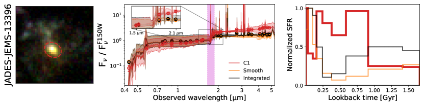
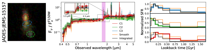
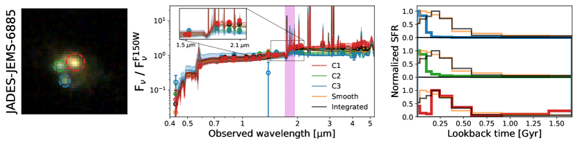
Figure 5: Spatially resolved stellar populations of the three galaxies with $z_{\rm{spec}}$. Left: The RGB images are the same as those shown in Figure 2, except that here we zoom in to the central 1.3”$\times$1.3” region. The middle and right panels show the SED fitting results from our fiducial Prospector model (Section 2.4). Middle: The normalized (i.e., F${}_{\nu}^{\rm{F150W}}=1$) photometry and best-fit SEDs of individual structural components defined in Section 2.3. These include best-fit SEDs for (1) visually identified clumpy substructures which are color-coded accordingly based on the colors used in the RGB images for individual apertures, (2) the Smooth component (orange) and (3) integrated flux (black). The inset highlights the wavelength range around 2$\micron$ covered by NIRCam F150W, F182M, F200W and F210M, and HST/WFC3 F160W filters. The magenta shaded region marks the rest-frame wavelength range between 3645 Å and 4100 Å which contains key spectral features sensitive to stellar age such as the Balmer jump and D4000 break (Bruzual A., 1983; Balogh et al., 1999). Right: Reconstructed nonparametric SFHs of individual substructures. Each SFH is normalized with its peak SFR, i.e., Normalized SFR(t) = SFR(t)/max(SFR(t)), to better show the difference in the shape of SFHs. In each subpanel, we overplot the best-fit nonparametric SFHs for the Smooth component (orange) and integrated flux (black). For better illustration, here we only plot the best-fit SFHs with solid lines, while in Appendix B we also plot the 1$\sigma$ uncertainties.

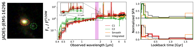
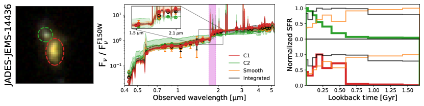
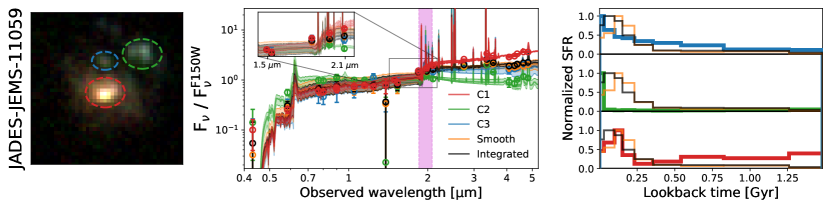
Figure 6: Similar to Figure 5, but for the three galaxies with $z_{\rm{phot}}$ shown in Figure 3. Note that the C2 of JADES-JEMS-11059 is not covered by its segmentation map (the bottom row of Figure 3), but we still include it to the analysis because its photometric redshift is consistent with that of the central galaxy.

3.2 Stellar Masses of the Substructures

The stellar mass of clumpy substructures contains key information on their physical origins (e.g., Dekel et al., 2009; Genzel et al., 2011; Guo et al., 2012; Bournaud et al., 2014; Guo et al., 2015; Dessauges-Zavadsky & Adamo, 2018). Directly comparing their stellar masses with the mass threshold of gravitational collapse due to local hydrodynamical instabilities ($M_{\rm{Toomre}}$, Toomre, 1964, see Section 3.3 for details) will immediately tell us that if their formation is consistent with in-situ fragmentation in gaseous disks.

Accurately measuring the stellar mass of clumps, however, is very challenging, because they are embedded in a smooth component, e.g., a galaxy disk. We thus need to properly subtract the contribution from the smooth component at the clump locations, otherwise the stellar-mass measures will be biased (Huertas-Company et al., 2020). In our case, this can be formularized as

$$\rm{M_{C}^{int}=\eta\cdot(M_{C}-M_{S}^{C}})$$ (4)

where $\rm{M_{C}^{int}}$ is the intrinsic (i.e., true) stellar mass of a clump; $\rm{M_{C}}$ is the stellar mass of that clump derived from SED fitting with fluxes directly from aperture photometry (Section 2.3 and Section 2.4); $\rm{M_{S}^{C}}$ is the contribution from the smooth component to the stellar-mass measure at the clump location and finally $\eta$ accounts for aperture correction.

Reliably estimating $\rm{M_{S}^{C}}$ and $\eta$ requires information on intrinsic shapes of clumps and the smooth component, which unfortunately are not known a priori, and it becomes increasingly challenging when clumps are fainter. However, we reiterate that the primary goal of this work is to understand the formation of massive stellar cores (i.e., C1), rather than to, e.g., measure the stellar-mass function of clumps. If the stellar mass of a clump is less than the threshold mass even before subtracting $\rm{M_{S}^{C}}$, i.e., $\eta M_{\rm{C}}<M_{\rm{Toomre}}$, its formation will then be fully consistent with in-situ fragmentation. Robustly determining the stellar masses for these low-mass, faint clumps (mostly C2 and C3) is beyond the scope of this paper, and in such cases we simply use $\eta M_{\rm{C}}$ as a strict upper limit (Figure 8 and Section 3.3).

In the remainder of this Section, the main focus will be on estimating intrinsic stellar masses of clumps (C1 in particular) more massive than $M_{\rm{Toomre}}$. We estimate them using two different empirical methods (Section 3.2.1 and 3.2.2), and with different aperture correction factors (Section 3.2.3). In short, our conclusion, that intrinsic stellar masses of C1 are larger than $M_{\rm{Toomre}}$, does not depend on the choice of method.

3.2.1 Estimating $\rm{M_{C}^{int}}$ by Directly Subtracting the Mass Contribution from the Smooth Component

As we showed earlier in Figure 4, because the coadded measurements of stellar mass and star formation rate are consistent with those derived using integrated flux, this supports our decision to perform the direct subtraction in mass. If we assume that the mass-to-light (M/L) ratio is constant and stellar mass is uniformly distributed within the Smooth component, then $\rm{M_{S}^{C}}$ simply is the stellar mass of the Smooth component derived via SED fitting using fluxes directly from aperture photometry ($\rm{M_{S}}$) and scaled by the area ratio of the clump (A_C) to the Smooth component (A_S). The intrinsic stellar mass of the clump is then

$$\rm{M_{C}^{int}=\eta\cdot\left(M_{C}-\frac{A_{C}}{A_{S}}M_{S}\right)}.$$ (5)

Because stellar masses of individual components were derived by SED fitting (Section 2.4), the biggest advantage of this approach is that the spatial variation in M/L has already been largely taken into account, despite not being on a pixel-by-pixel basis. In Figure 8, we plot the resulting $\rm{M_{C}^{int}}$ as filled symbols with error bars. For all C1, we find $\rm{M_{C}^{int}/M_{Toomre}\gtrsim 2}$, arguing against formation via in-situ fragmentation. We use the intrinsic stellar masses of C1 derived from this approach as the fiducial ones for the discussion in Section 4.

3.2.2 Estimating $\rm{M_{C}^{int}}$ by Subtracting the Flux Contribution from the Smooth Component

Differing from directly subtracting mass, alternatively we can first subtract the flux contribution from the Smooth component to the clump location, and then estimate $\rm{M_{C}^{int}}$. The Equation (4) thus becomes

$$\rm{M_{C}^{int}=\eta\cdot\left(M_{C}-\frac{A_{C}\cdot f_{S}^{C}}{F_{C}}M_{C}\right)}$$ (6)

where $\rm{f_{S}^{C}}$ is the flux contribution per pixel from the Smooth component to the clump location, and $\rm{F_{C}}$ is the flux of the clump from aperture photometry.

For each one of the galaxies, we estimate $\rm{f_{S}^{C}}$ by subtracting from its F210M image the best-fit forcepho models (Section 2.5) of all clumpy substructures. We then do a 3$\sigma$ clipping on the residual image and use the median residual pixel value as $\rm{f_{S}^{C}}$. Because we ignore the Smooth component during the forcepho fitting (Section 2.5), instead of using the residual image, we also estimate $\rm{f_{S}^{C}}$ in a more aggressive way. We first mask out pixels within $r=2\times$R_e circular regions of individual clumpy substructures from the galaxy’s segmentation map, and then estimate $\rm{f_{S}^{C}}$ as the median pixel value of the masked image (i.e., without subtracting the best-fit forcepho models of clumpy substructures). This latter estimate certainly overestimates $\rm{f_{S}^{C}}$ because the flux contribution from clumps to the Smooth component is not fully removed. Even so, we find that $\rm{f_{S}^{C}}$ only increases by $\sim 3-7\%$, which is small and will not cause any substantial changes in our results.

In Figure 8, we use hollow symbols with dashed edges to show the $\rm{M_{C}^{int}}$ of C1 from this approach. The $\rm{M_{C}^{int}}$ from this approach are larger than the fiducial ones, which is expected because Equation 6 assumes the same M/L for C1 and the Smooth component. As Figure 5 and 6 show, in each one of the galaxies, C1 has a redder rest-frame (B $-$ V) color, as probed by F182M $-$ F277W, than the Smooth component. Because M/L increases as (B $-$ V) becomes redder (e.g., McGaugh & Schombert, 2014), using Equation 6 can lead to an under-subtraction of $\rm{M_{S}^{C}}$. This issue can be mitigated by doing the forcepho analysis across all filters, as opposed to only using the F210M filter, and then taking the M/L variation into account with the forcepho-derived model photometry. Following this, we find that the intrinsic masses of C1 can change by $\lesssim 20\%$, a sufficiently small amount that does not substantially change any of our results.

3.2.3 Estimating the Aperture Correction Factor $\mu$

By default, we use the best-fit Sérsic profile from the forcepho fitting (Section 2.5) to derive the aperture correction factor $\mu$. As the posterior plots of Figure 7 show, the Sérsic profiles of C1 are tightly constrained, with typical uncertainties of Sérsic index $n$ and effective radius R_e of $<10\%$. C1 are resolved/marginally resolved in NIRCam/F210M images (PSF FWHM $\approx 0^{\prime\prime}.07$), spanning a range in R_e of $0^{\prime\prime}.07-0^{\prime\prime}.14$, corresponding to $0.5-1$ kpc at the median redshift $\bar{z}=3.7$. For minor clumps C2 and C3, their Sérsic profiles are much less constrained. We also check our results by adopting a rather conservative aperture correction, namely, assuming the clumps are point sources, which we already knew does not accurately describe C1’s morphologies. Using the point source aperture correction can lead to a decrease in stellar mass by a factor of $\sim 1.5-2.1$, which, still, cannot substantially change our conclusions because all C1 have $\rm{M_{C}^{int}/M_{Toomre}\gtrsim 2}$ (see Figure 8 and Section 3.3 below).

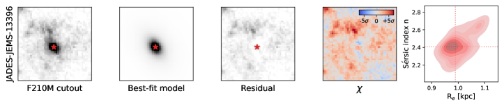
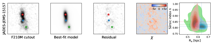
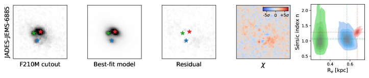
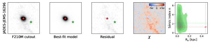
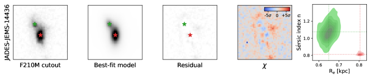
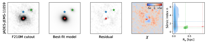
Figure 7: Morphological analysis for the individual substructures. Each substructure is modelled as a Sérsic profile using the code forcepho that adopts an MCMC framework to perform PSF-convolved analysis in individual exposures to better estimate the parameter uncertainties (Section 3.2). The best-fit centroids of individual substructures are marked with the star symbols. The left three columns show the F210M cutout, best-fit model and residual, respectively. The fourth column shows the residual $\chi$ map, which is defined as $\chi=$ (data $-$ model)/error, from which we clearly see the Smooth component surrounding the clumpy substructures. The last column shows the posterior corner plot of Sérsic index $n$ vs circularized effective (i.e., half-light) radius R_e.

3.3 Origins of the Substructures

A prominent feature of high-redshift galaxies is the presence of giant stellar clumps which are far more massive than individual star clusters observed in nearby galaxies (e.g., Elmegreen et al., 2007; Genzel et al., 2008, 2011; Guo et al., 2012, 2018; Wuyts et al., 2012). One scenario to form such giant clumpy substructures is through in-situ fragmentation due to violent disk instabilities (e.g., Noguchi, 1999; Immeli et al., 2004; Bournaud et al., 2007; Elmegreen et al., 2008; Dekel et al., 2009; Ceverino et al., 2010; Inoue et al., 2016). In a rotating gaseous disk, gravity needs to overcome both gas pressure and shear forces produced by the relative motion between fluid parcels. Toomre (1964) showed that in-situ fragmentation can happen if the parameter $Q$ is less than unity (Section 1). Consequently, clumps have a characteristic mass which represents the largest stellar mass that a clump can form via Toomre instability, a.k.a. the Toomre mass. Following Genzel et al. (2011), the Toomre mass can be calculated as

$$M_{\rm{Toomre}}\approx 5\times 10^{9}\left(\frac{f_{\rm{young}}}{0.4}\right)^{2}\left(\frac{M_{\rm{disk}}}{10^{11}M_{\sun}}\right)M_{\sun}$$ (7)

where $f_{\rm{young}}$ is the mass fraction of components forming stars and $M_{\rm{disk}}$ is the total baryonic mass of a disk.

To estimate $M_{\rm{Toomre}}$ for our sample, we assume $f_{\rm{young}}\approx f_{\rm{gas}}$, where $f_{\rm{gas}}$ is the gas-to-baryonic mass fraction, i.e., $M_{\rm{gas}}/(M_{\rm{gas}}+M_{*})$. Strictly speaking, $M_{\rm{gas}}$ here should be the summation of molecular and atomic gas masses in galaxy disks, but we assume $M_{\rm{gas}}\approx M_{\rm{molgas}}$ for the following reason. While directly measuring atomic gas in galaxies beyond the local universe is technically challenging, studies using the damped Lyman-alpha absorbers toward high-redshift quasars infer a generally very weak, if any, evolution of the cosmic atomic Hydrogen density ($\rho_{\rm{HI}}$) up to $z\sim 5$ (e.g., Rao et al., 2006; Prochaska & Wolfe, 2009; Péroux & Howk, 2020; Walter et al., 2020). Meanwhile, observations with different probes of molecular gas, including CO, FIR SED and sub-mm dust continuum, have reached a consensus, at least up to $z=4$, that the molecular-gas mass of galaxies rapidly evolves at a rate of $(1+z)^{3\pm 1}$ (e.g., Genzel et al., 2015; Scoville et al., 2017; Tacconi et al., 2018; Liu et al., 2019). Putting together the weak $\rho_{\rm{HI}}$ and strong molecular-gas evolutions, because the mass ratio of atomic gas divided by molecular gas is $\approx 2-3$ at $z\sim 0$ (e.g., Saintonge et al., 2011; Catinella et al., 2013), it is reasonable to assume $M_{\rm{gas}}\approx M_{\rm{molgas}}$ (hence $f_{\rm{gas}}\approx f_{\rm{molgas}}$) in galaxies at $z\gtrsim 1$ (see a similar argument from Tacconi et al. 2018 for this assumption).

We estimate $f_{\rm{molgas}}$ for the 6 galaxies using the best-fit relationship from Tacconi et al. (2020) (their Equation 2), who combined a number of surveys of galaxies’ molecular gas content across cosmic time, and also included the dependence of the relationship on stellar mass and the distance to the star-forming main sequence. We note, however, that almost all those high-redshift surveys were designed for galaxies with M${}_{*}>10^{10}M_{\sun}$, either on or above the star-forming main sequence. Because 5 out of the 6 galaxies presented in this work have M${}_{*}\approx 10^{9.3-10}M_{\sun}$ (Table 1), we use the $f_{\rm{molgas}}$ derived for M${}_{*}=10^{10}M_{\sun}$ galaxies. As we will show in Section 4.2, all 6 galaxies are below the star-forming main sequence. Using their distances to the star-forming main sequence, we find $f_{\rm{gas}}\approx 0.5$ for our sample, similar to those observed in star-forming galaxies on the main sequence at $z\sim 2$ (e.g., Tacconi et al., 2008, 2010; Daddi et al., 2010). With $f_{\rm{gas}}$ in hand, we then get $M_{\rm{disk}}=M_{*}+M_{\rm{gas}}=M_{*}/f_{\rm{gas}}$, and finally use Equation 7 to calculate $M_{\rm{Toomre}}$. In Figure 8, we plot the relationship between $M_{\rm{Toomre}}$ and $M_{*}$ as the black solid line. In what follows, we discuss possible physical origins of the clumpy substructures.

To begin, Figure 8 shows that the most minor clumps (C2 and C3) are less massive than $M_{\rm{Toomre}}$, hence they are consistent with in-situ formation through gravitational fragmentation in gaseous, turbulent disks. These clumps are bluer, and have enhanced specific star formation rates compared to C1 and the Smooth component (Table 2). These properties are similar to the star-forming clumps found in galaxies at lower redshifts $1<z<3$ from earlier HST studies (e.g., Elmegreen & Elmegreen, 2005; Elmegreen et al., 2007; Wuyts et al., 2012). Quantitatively, these individual minor clumps contribute $5-50\%$ of the total star formation rate, and $<10\%$ of the total stellar mass of their host galaxies, in broad agreement with earlier studies of UV-bright clumps at $1<z<3$ (e.g., Guo et al., 2012). In addition, they have overall rising SFHs started $\approx 0.3$ Gyr ago, which is also consistent with the young stellar ages found in $2<z<3$ star-forming clumps (Elmegreen et al., 2009; Förster Schreiber et al., 2011; Genzel et al., 2011; Guo et al., 2018).

Apart from C1, two other clumpy substructures are more massive than $M_{\rm{Toomre}}$, i.e., the C3 of JADES-JEMS-15157 (blue X in Figure 8) and the C2 of JADES-JEMS-14436 (green hexagon in Figure 8). Regarding the former, its intrinsic stellar mass is $\sim 1.5\times$ $M_{\rm{Toomre}}$. We notice, however, that it might contain two distinct clumps, which is particularly clear in the F210M image but becomes less obvious in other filters (Figure 2). After taking this into account, its formation is then still consistent with in-situ fragmentation. Regarding the latter, i.e. the C2 of JADES-JEMS-14436, we see a clear tidal feature associated with this substructure in the NIRCam SW’s filter images (Figure 3 and Appendix C). Therefore, the physical origin of this substructure is very likely related to a minor merger with a mass ratio of 1:10 (Table 2). The minor mergers can have two broad effects on the clump formation. First, minor mergers can disturb the gas distribution in galaxy disks, trigger local starbursts and hence induce clump formation (Bournaud et al., 2014; Inoue et al., 2016). Second, the clumps can be minor mergers themselves, i.e., the clumps have an ex-situ origin. Using cosmological hydrodynamical simulations, Mandelker et al. (2014) found that the ex-situ clumps have a typical stellar age of $0.5-3$ Gyr and specific star formation rate of $0.1-2$ Gyr^-1, which are in quantitative agreement with the C2 of JADES-JEMS-14436 (Figure 6 and Appendix C).

Finally, at the core of this study is the physical origin of C1 – the dominated clumpy substructure. In each one of the 6 galaxies, C1 is redder than the other parts of the galaxy, and has significantly larger stellar mass than $M_{\rm{Toomre}}$, with a typical ratio of $\rm{M_{C}^{int}/M_{Toomre}\gtrsim 2}$. This excessive stellar mass is strong evidence that C1 may not formed via in-situ fragmentation in gaseous disks. Relative to those minor clumps discussed above, C1 has a lower specific star formation rate and is closer to the light centroid of NIRCam images at $\sim 4\micron$. All these are consistent with C1 being a forming stellar core/(pseudo-)bulge, which will be discussed in detail in the remainder of this paper.

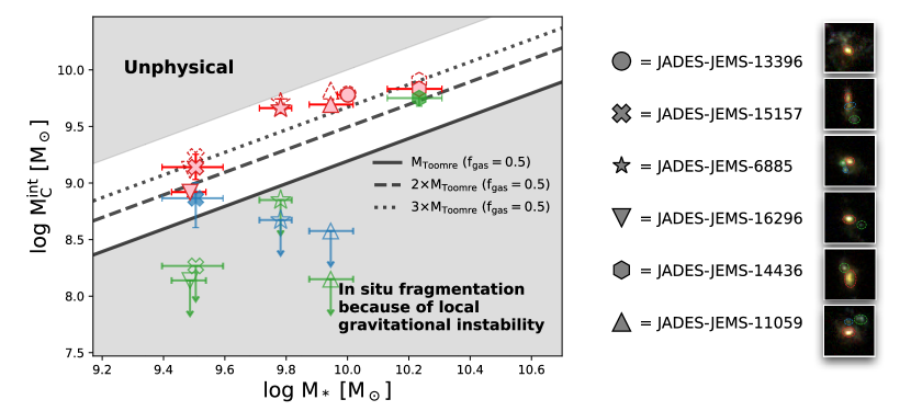
Figure 8: The scatter plot of the intrinsic stellar masses of clumpy substructures ($y$-axis) vs. the total stellar masses of their host galaxies ($x$-axis). The black solid line marks the prediction of Toomre mass $M_{\rm{Toomre}}$, which represents the largest stellar mass that a clump can form through Toomre instability in an unstable, gaseous disk (see Section 3.3). The dashed and dotted lines mark $2\times$ and $3\times M_{\rm{Toomre}}$, respectively. The upper-left grey shaded region marks the unphysical part where $\rm{M_{C}^{int}>M_{*}}$. The symbols used for individual galaxies, as well as the corresponding color scheme used for individual clumpy substructures are labelled on the right. For low-mass clumps whose stellar masses are already less than $M_{\rm{Toomre}}$ before subtracting the contribution from the surrounding smooth component (Section 3.2), we plot the upper limits of their $\rm{M_{C}^{int}}$. Similar to previous plots, the stellar cores C1 are color-coded in red. The filled symbols with error bars show the $\rm{M_{C}^{int}}$ estimated via the method of Section 3.2.1, while the hollow symbols with dashed edges show the $\rm{M_{C}^{int}}$ estimated via a different method described in of Section 3.2.2. We find that the intrinsic stellar masses of C1 are significantly larger than $M_{\rm{Toomre}}$ in all the six galaxies, suggesting that C1 may not form through in-situ fragmentation due to Toomre instability.

4 Discussion

4.1 The Formation of C1: Early (Pseudo-)Bulge Formation?

In the local universe, bulges and pseudo-bulges are believed to have different origins, with the former primarily formed through major mergers (e.g. Hernquist, 1989; Barnes & Hernquist, 1996; Hopkins et al., 2009) and the latter formed through secular evolution in galaxy disks (e.g. Debattista et al., 2004; Okamoto, 2013; Athanassoula et al., 2015). According to the classification for $z\sim 0$ galaxies, the light distribution of a classic bulge is similar to a spheroid ($n=4$), while it becomes flattened (smaller $n$) for a pseudo-bulge (Kormendy & Kennicutt, 2004). Therefore, from a purely morphological perspective (Figure 7), the C1 of JADES-JEMS-13396 ($n>2$) is more like a classic bulge, while in the other 5 galaxies C1 are consistent with pseudo-bulges, although we stress that without dynamical measures it remains difficult to definitively distinguish the two.

At high redshifts, early numerical simulations showed that stellar cores formed through the coalescence of in-spiral stellar clumps should have $n\sim 2-4$, being consistent with classic bulges (Elmegreen et al., 2008). Later simulations however, after taking into account the gas kinematics of individual clumps, showed that the remnant of the clump coalescence should still have significant rotation, arguing that the high-redshift cores are more consistent with being pseudo-bulges (Ceverino et al., 2012; Inoue & Saitoh, 2012). Regardless, those simulations consistently showed that the coalescence of clumps is an efficient way to grow dense central cores in gas-rich galaxies at high redshifts. Indeed, the coexistence of C1 with other minor, off-center star-forming clumps (C2 and C3) in the 6 galaxies is consistent with this picture.

The reconstructed SFHs provide another key constraint on the physical origin of C1. If they form through the coalescence of in-spiral clumps, the timescale for the clumps’ inward migration will be $\approx 0.5$ Gyr (e.g., Noguchi, 1999; Immeli et al., 2004; Bournaud et al., 2007; Genzel et al., 2008, 2011). This is consistent with the SED fitting that the mass-weighted stellar ages of C1 span a range of $0.4-0.7$ Gyr (Section 3.1). The clump migration scenario also predicts the radial age gradient of clumps. Indeed, those off-center minor clumps (C2 and C3, if present) have significantly younger SFHs (Figure 5 and 6), spanning a range in mass-weighted stellar age of $0.1-0.5$ Gyr (Table 2). These are in quantitative agreement with the model from Dekel et al. (2009) which predicts that clumps should have stellar ages $<0.5$ Gyr at the outskirt while they are older at the center.

One important question about the efficacy of the inward migration scenario is the uncertain lifetime of clumps. Can clumps formed in disks survive stellar feedback until they coalesce at the center? Some simulations with intense stellar feedback models showed that clumps are short-lived, and should be self-destroyed within $<50-100$ Myr (Genel et al., 2012; Hopkins et al., 2012). In contrast, other simulations with different stellar feedback models showed that they can produce relatively longer-lived stellar clumps with a typical age of a few hundred Myr (Perez et al., 2013; Bournaud et al., 2014; Ceverino et al., 2014). The stellar ages of $0.1-0.5$ Gyr measured for the minor clumps C2 and C3 favor a relatively longer lifetime of clumps than the predictions from intense stellar feedback models, similar conclusions were also reached by earlier studies of $z\sim 2$ star-forming clumps (Wuyts et al., 2012; Guo et al., 2012). Arguably, however, the measured stellar ages of C2 and C3 still seem to be shorter than the $\approx 0.5$ Gyr required for the inward migration. As pointed out by Bournaud (2016), however, the observed stellar ages of clumps are only lower limits to their true ages, because during their evolution clumps continuously exchange mass with the surrounding ISM through outflows and inflows (Bournaud et al., 2007; Dekel & Krumholz, 2013; Bournaud et al., 2014; Perret et al., 2014). According to the zoom-in simulations from Bournaud et al. (2014), a clump with an observed stellar age of $0.1-0.2$ Gyr corresponds to a true age of $0.3-0.5$ Gyr. Taking this into account, the inferred stellar populations for the minor clumps thus are still in line with the scenario where the central regions of high-redshift galaxies are built through the in-spiral of clumps.

We also note that major mergers, if present, can help efficiently grow central cores/bulges at high redshifts as well. However we do not see clear evidence of major mergers in the 6 galaxies presented here. The effect induced by recent minor mergers, e.g., the formation of bars, can also contribute to the buildup of (pseudo-)bulges (e.g., Bournaud et al., 2005; Eliche-Moral et al., 2011; Guedes et al., 2013). Given the complex morphologies of the galaxies, however, it is hard to distinguish an in-situ stellar clump from a merging low-mass galaxy. Minor mergers thus might also contribute to the development of central regions in the six galaxies.

Finally, we notice that C1 has a comparable/younger mass-weighted stellar age than the Smooth component in each one of the galaxies (Table 2). As the reconstructed SFHs show (see Figures 5 and 6), this is because the Smooth component started its major mass assembly either at about the same time as C1, or earlier, i.e., $>1$ Gyr prior to the time of observation. Interestingly, recent studies of galactic archaeology found that the Milky Way’s bulge is predominately composed of $\gtrsim 9-10$ Gyr-old stars (corresponding to a formation redshift $z\gtrsim 2-3$, e.g., Barbuy et al., 2018; Hasselquist et al., 2020), while the formation of thick-disk stars likely started as early as at $z>6$, i.e. 13 Gyr ago (Xiang & Rix, 2022). These are seemingly similar to the reconstructed SFHs of C1 and the Smooth component. It is thus possible that we are witnessing the early formation of structural components that will eventually evolve into the bulge and thick-disk components in the Milky Way-like galaxies at $z\sim 0$, although we caution that the 6 galaxies are likely hosted by dark matter halos $\approx 0.5-1.5$ dex more massive than the Milky Way’s.

4.2 Implications for Galaxy Quenching

We now advance the discussion by connecting what we found about the 6 galaxies to the general picture of galaxy quenching.

To begin, in Figure 9 we present the star-forming main sequence, i.e. star formation rate vs stellar mass, for all 301 galaxies at $3<z<4.5$ in our parent sample from JEMS (Section 2.1). The star formation rate and stellar-mass measures shown in the plot are from our Prospector SED fitting with the same model as that assumed for the 6 galaxies (Section 2.4), measured with integrated flux. We compare the star-forming main sequence with that from Popesso et al. (2023) who conducted a comprehensive literature search, and used a consistent method to derive the star-forming main sequence over $1<z<6$ for galaxies with $M_{*}>10^{8.5}M_{\sun}$. As Figure 9 shows, our measurements are in excellent agreement with the distribution measured by Popesso et al. (2023). We also plot the star-forming main sequence from Leja et al. (2022), who also used Prospector with a very similar SED model to ours, but only measured the relation for galaxies up to $z=2.7$ with $M_{*}>10^{10.2}M_{\sun}$ owing to the stellar-mass incompleteness. As Figure 9 shows, the 6 galaxies presented in this work are below the star-forming main sequence by $0.2-0.7$ dex, suggesting a possible link between the presence of a massive stellar core (e.g., C1) and galaxy quenching.

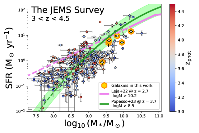
Figure 9: The star-forming main sequence of $3<z<4.5$ galaxies from JEMS. The stellar mass and star formation rate are derived from SED fitting with integrated flux. Each galaxy is color-coded using its best-fit photometric redshift. The green solid line shows the star-forming main sequence at $z=3.7$ for $M_{*}>10^{8.5}M_{\sun}$ galaxies from Popesso et al. (2023). We extrapolate it to $M_{*}<10^{8.5}M_{\sun}$, and plot it as the green dashed line. The green shaded region marks the $\pm 0.3$ dex range. Also plotted as the magenta solid line is the star-forming main sequence at $z=2.7$ for $M_{*}>10^{10.2}M_{\sun}$ galaxies from Leja et al. (2022), who also used Prospector with a similar SED model of this work. Similarly, we also extrapolate it to $M_{*}<10^{10.2}M_{\sun}$, and plot it as the magenta dashed line. The six galaxies presented in this work are marked with golden hexagons. They are below the star-forming main sequence by $\approx 0.2-0.7$ dex.

In Figure 10, we continue the discussion by comparing the stellar-mass surface densities at the location of C1 ($\rm{\Sigma_{C1}}$) with the prediction based on the evolution of $\Sigma_{\rm{1kpc}}$, i.e., the stellar-mass surface density within the central radius of 1 kpc, of $0.5<z<3$ galaxies measured by Barro et al. (2017) using HST data from CANDELS. Specifically, we compare with the $\Sigma_{\rm{1kpc}}$ evolution of star-forming (the cyan line in Figure 10) and quiescent (the magenta line in Figure 10) galaxies with $M_{*}=10^{9.7}M_{\sun}$, i.e., the median stellar mass of the galaxies presented in this work.

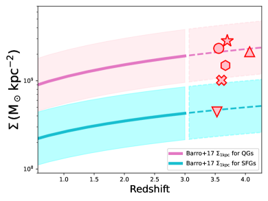
Figure 10: The stellar-mass surface density at the location of C1. The symbol used for each galaxy is the same as Figure 8. The solid line shows the $\Sigma_{\rm{1kpc}}$ evolution of galaxies at $0.5<z<3$ measured by Barro et al. (2017). We extrapolate this evolution to $z>3$ and plot it as the dashed line. The evolution of star-forming galaxies and quiescent galaxies is plotted in cyan and magenta, respectively. The shaded region marks the $\pm 0.3$ dex range. Although the six galaxies have not quenched yet, their stellar-mass densities within the region of C1 are already high, approaching the central stellar-mass surface density of high-redshift quiescent galaxies (see Section 4.2 for detailed discussions and caveats of this comparison).

Before proceeding to discuss the results, we clarify how we estimate $\rm{\Sigma_{C1}}$ for a fair comparison with the existing $\Sigma_{\rm{1kpc}}$ measures, and caution about the caveats in this comparison. First, because C1 are close to the center of stellar-light distributions (NIRCam images at $\sim 4\micron$ in Figure 2 and Figure 3), and their sizes are $\approx 0.5-1$ kpc (effective radius, Figure 7), $\rm{\Sigma_{C1}}$ is a good proxy for the central stellar-mass surface densities of the galaxies presented in this work. Second, we note that the existing $\Sigma_{\rm{1kpc}}$ measures simply assumed a single Sérsic profile for the entire galaxy, meaning that those $\Sigma_{\rm{1kpc}}$ measures included all stellar masses in the central regions, regardless of their origins (e.g., cores vs stars in disks). For a fair comparison, instead of using $\rm{M_{C1}^{int}}$ (Equation 4), we thus include all masses at the location of C1, i.e., $\rm{\Sigma_{C1}=\eta M_{C1}/A_{C1}}$, where $\rm{A_{C1}}$ is the aperture size used for C1. Third, the earlier studies were only able to study the evolution of $\Sigma_{\rm{1kpc}}$ up to $z=3$. In this work, we therefore need to extrapolate the $\Sigma_{\rm{1kpc}}$ evolution from Barro et al. (2017) to a higher redshift range, i.e., $3<z<4.5$. Finally, at $z\sim 3$, while the stellar-mass completeness of CANDELS is still $\sim 10^{9.5}M_{\sun}$ for star-forming galaxies (e.g., Ji et al., 2018; Santini et al., 2022), it rises to $\sim 10^{10.3}M_{\sun}$ for quiescent galaxies (Barro et al., 2017). We therefore also need to extrapolate the $\Sigma_{\rm{1kpc}}$ evolution for quiescent galaxies from Barro et al. (2017) to a lower stellar mass $10^{9.7}M_{\sun}$.

As Figure 10 shows, except JADES-JEMS-16296, all the other 5 galaxies have large central stellar-mass surface densities, namely, that their $\rm{\Sigma_{C1}}$ are already similar to the $\Sigma_{\rm{1kpc}}$ of quiescent galaxies of similar redshifts and masses. Interestingly, JADES-JEMS-16296 in fact is the galaxy that shows evidence of recent rejuvenation of central star formation which will be further discussed in Section 4.3. Although the galaxies presented in this work are not quenched yet, they are below the star-forming main sequence. On the one hand, although we cannot be sure that these 6 galaxies will not rejuvenate their star-formation activities in the future, the findings here suggest that galaxies have already formed significant amount of their mass in a spheroidal central component while they are still in the star-forming phase, which is consistent with what has been found in the IllustrisTNG simulations (Pillepich et al., 2019; Tacchella et al., 2019). On the other hand, it is also possible that the galaxies are actually heading toward quiescence. The presence of a massive stellar core with a surface density comparable to quenched galaxies then suggests that the suppression of star formation may occur along with the development of dense central regions. The implication is that there is either a causal link between quenching and central structural transformations, or an as-yet unidentified physical process that controls both events.

The conclusion above is in broad agreement with the studies at lower redshifts (e.g. Fang et al., 2013; Barro et al., 2017; Whitaker et al., 2017; Tacchella et al., 2018; Suess et al., 2021; Ji & Giavalisco, 2023). What is different here, though, is that we are now able to study the buildup of central regions in the act at $3<z<5$ in the progenitor of lower-redshift massive quiescent galaxies, thanks to the deep NIRCam imaging obtained by JADES and JEMS. This, in our view, is an important step forward because those lower-redshift quiescent galaxies are already old – the typical stellar age of $z\sim 1-2$ massive quiescent galaxies is about 1 Gyr (e.g., Carnall et al., 2019b; Tacchella et al., 2022a; Ji & Giavalisco, 2022). This fact complicates the interpretation for the correlation between the star-formation properties and central stellar-mass surface density that is well established at $z=1-2$ (e.g. Belli et al., 2015; Williams et al., 2017; Estrada-Carpenter et al., 2020), because post-quenching processes can alter galaxies’ structures. Thus, it is difficult to assess if the correlation is really due to a causal link between the development of dense cores and quenching, or is simply a byproduct of another yet-to-be identified physical process. Pushing observations closer to higher redshifts $z>3$, i.e. closer to the time of quenching, enables a more direct view of the relative timing between structural transformations and quenching, hence guarantees a more accurate constraint on the relationship between the two phenomena.

4.3 Consistency between our Observations and the Gas-rich Compaction Scenario

Finally, we discuss our constraints on the physical mechanisms responsible for the correlation between the star-formation properties and central stellar-mass surface density observed in galaxies at cosmic noon (e.g., Franx et al., 2008; Cheung et al., 2012; Whitaker et al., 2017; Barro et al., 2017). Our observations are fully in line with the so-called “gas-rich compaction” scenario, which actually is a class of processes whose main feature is highly dissipative gas accretion toward the center of galaxies. This process promotes enhanced central star-formation activity, followed by the central gas depletion and finally the quenching of central star formation (Dekel et al., 2009; Ceverino et al., 2010; Dekel & Burkert, 2014; Wellons et al., 2015; Zolotov et al., 2015; Tacchella et al., 2016).

One important prediction of gas-rich compaction is that, right after a compaction event, we should observe a younger stellar population at the center as a result of recent central starburst triggered by the highly dissipative gas accretion. This is observed in the 6 galaxies where C1 are comparable to/younger than the Smooth component (Section 3.1). Additionally, we find that C1 feature a common SFH whose star formation rate declines over the past $0.1-0.3$ Gyr, following a major star-forming episode $\approx 0.5-1$ Gyr prior, and peaked $\approx 0.2-0.5$ Gyr ago. This SFH is consistent with the 6 galaxies experiencing a gas compaction event, followed by a suppression of star formation likely as the result of central gas depletion. If there is future gas replenishment, this chain of events, i.e. gas compaction followed by gas depletion, will repeat several times before the final quiescence of the entire galaxy at $z<3$ (Tacchella et al., 2016). Indeed, we see evidence of star-formation rejuvenation in the C1 of JADES-JEMS-16296 by the time of observation. This rejuvenation event happens at $\approx 0.3$ Gyr after the peak of the galaxy’s most recent major star-formation episode. Interestingly, this timescale is very similar to the model predictions for the oscillation timescale ($0.2-0.5\,{\rm{t_{H}}}$, corresponding to $0.3-0.8$ Gyr at $z=3.7$) of star formation triggered by gas replenishment (Tacchella et al., 2016). However, we caution that this result is sensitive to the assumed prior of nonparametric SFHs (see Appendix B).

5 Summary

This is the first paper of the series that uses deep 14-filter JWST/NIRCam imaging data from the JEMS and JADES surveys to study in detail the spatially resolved stellar populations of galaxies at redshifts $3<z<4.5$, a key epoch of the universe that can provide unique insight into the role that substructures among massive galaxies may play in the transition from star-forming disks to bulge-dominated, quiescent galaxies.

We visually inspected color maps at rest-frame $3600-4100$ Å produced by JWST/NIRCam imaging for all $3<z<4.5$ galaxies in JEMS, from which we identified a sample of 37 galaxies having substructures with distinct rest-frame colors. These 37 galaxies show diverse spatially resolved stellar populations. In this first paper, we present the spatially resolved stellar populations in 6 galaxies with massive stellar cores, representing a specific stage of galaxy structural transformation.

We divided each one of the 6 galaxies into different structural components, including (1) a bright central stellar core C1, the focus of this study, (2) off-center, minor clumps C2 and C3 (if present), and (3) the Smooth component representing the remaining, extended light distribution of the galaxy. Together with 9-filter ancillary imaging from HST, we fit a total of 23-filter photometry covering truly panchromatic swathes of observed wavelength range $\lambda=0.4-5\micron$, corresponding to the rest-frame $0.1-1\micron$, using the SED fitting code Prospector with nonparametric SFHs. We then studied the stellar-population properties of those different structural components.

In each one of the galaxies, C1 has a redder color at rest-frame 4000 Å and a significantly lower specific star formation rate than off-center clumps C2 and C3. We showed that C1 is $\gtrsim 2$ times more massive than $M_{\rm{Toomre}}$, i.e., the maximum stellar mass that a clump can form via Toomre instability, suggesting that it may not have formed via in-situ fragmentation in an unstable, gaseous disk. Instead, because C1 has a typical stellar age of $\sim 0.5$ Gyr which is similar to the timescale of clump inward migration as the result of dynamical friction, we argued that C1 likely formed through the coalescence of giant stellar clumps.

We found that all 6 galaxies are below the star-forming main sequence by $0.2-0.7$ dex. We showed that the stellar-mass surface densities of C1 are already comparable to the central stellar-mass surface density of quenched galaxies of similar masses and redshifts. In addition, we found that the stellar populations of C1 are either comparable to or younger than the Smooth component. Putting these together, we thus concluded that we are likely witnessing the coeval development of dense central cores, along with the beginning of galaxy-wide quenching at $z>3$, likely triggered by gas-rich compaction.

As a closing remark, we stress that the sample presented here only contains 6 galaxies and hence has no statistical power. In addition, the visual selection means that this study is biased toward bright substructures in relatively bright galaxies. To obtain a robust statistical characterization of massive stellar cores in high-redshift galaxies, and a comprehensive picture of its relationship with quenching, a much larger sample with a more uniform selection method is required. We, however, view this work as a pilot study to demonstrate the power of JWST, especially its imaging capability with NIRCam, in constraining the spatially resolved mass assembly history of galaxies at $z>3$ in unprecedented detail. We reiterate that the galaxies here were selected from JEMS, whose sky coverage is relatively small ($\sim 10$ arcmin²). The ongoing JADES survey will eventually produce NIRCam imaging and NIRSpec spectroscopy of similar depth over a sky area of $\gtrsim 200$ arcmin² in the GOODS fields, promising a statistically significant galaxy sample at $z>3$ that will dramatically advance our understanding of the physics of galaxy structural transformation and quenching in the early universe.

Appendix A Comparing effective PSF with webbpsf-predicted model PSF

Knowledge of the Point Spread Function (PSF) plays an essential role in getting accurate PSF-matched aperture photometry, and hence the inferences of physical properties of stellar populations. Per JWST User Documentation, NIRCam’s PSFs are under-sampled in both $<2\micron$ SW filters and $<4\micron$ LW filters. To overcome this, we have constructed empirical and theoretical PSF models for JADES and JEMS with the following three different approaches:

• Effective PSF (ePSF) – We construct ePSFs using the EPSFBuilder in Photutils, which adopts the empirical method from Anderson & King (2000) to iteratively solve the centroids and fluxes of a list of input point sources, and then stack them together. For the list of point sources, we visually selected 13 isolated point sources from JADES and JEMS. These point sources are bright, but unsaturated across all NIRCam filters used in this study.

• Model PSF (mPSF) – Two effects are taken into account during the construction of mPSFs. The first effect comes from instrumental responses, which are taken care by the software Webbpsf. The other effect comes from data reduction, especially from the mosaicking process. To include both effects to the mPSF construction, we assume a list of synthetic point sources with known WCS coordinates. For each one of the point sources, we first project its WCS coordinate to individual exposures. In each exposure, we then convert the WCS coordinate to the corresponding detector coordinate, and use the Webbpsf to predict the PSF at that location, during which we adopt the JWST on-orbit measured Optical Path Difference (OPD) map closest to the date of that exposure. We repeat these for all synthetic point sources. Finally, we use the mosaicking pipeline of JADES to combine individual exposures together and get the mosaicked PSF images. We have made the PSF mosaics for all NIRCam filters used in this work (three examples are shown in Figure 11). These mosaics allow us to check astrometric accuracy, image quality and to study the spatial variation of PSFs, which will be presented in detail in Ji et al 2023 in preparation.

• Simple Webbpsf – Unlike mPSFs, simple Webbpsf models do not include any observational and data reduction effects.

In Figure 12 and 13, we compare the above three PSF models. Excellent agreement is seen between ePSFs and mPSFs, with a typical difference of $\lesssim 1\%$ in radial profiles of enclosed energy. We have tested our PSF-matched photometry using the mPSFs, and found no substantial changes at all for the results of this paper.

We note, however, that the analysis here demonstrates that simple Webbpsf models can significantly deviate from ePSFs, especially at small angular scales of $<0.1$ arcsec. Therefore, using simple Webbpsf models can lead to significant systematics in the PSF-related analysis, if observational and data reduction effects are not taken into account. Once these effects are properly modelled, the prediction of Webbpsf is very accurate. This last point is very important for extragalatic deep surveys like JADES, whose observational configurations (e.g. dithering patterns) can be complex and where not enough high S/N, unsaturated stars are in the field for constructing high-quality ePSF models to large angular scales.

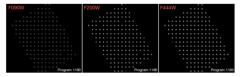
Figure 11: JADES PSF mosaics of NIRCam/F090W (left), F200W (middle) and F444W (right) filters produced following the procedure described in Appendix A.

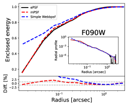
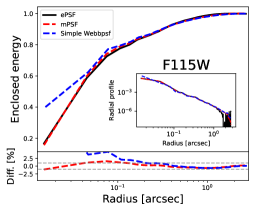
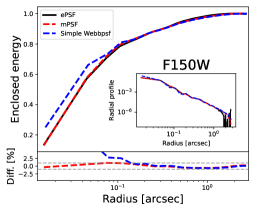
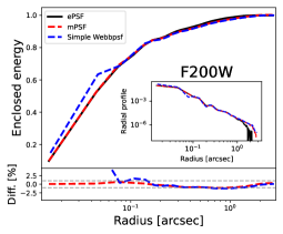
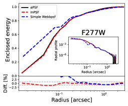
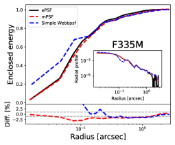
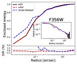
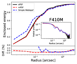
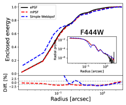
Figure 12: Comparisons among three different PSF models (Appendix A) for the NIRCam filters used by JADES. Plotted in the bottom of each panel are the differences between mPSFs and ePSFs (red dashed line), and between simple Webbpsf models and ePSFs (blue dashed line), where the horizontal, grey dashed lines mark $\pm 1\%$ range. Excellent agreement is observed between ePSFs and mPSFs, while simple Webbpsf models significantly deviate from ePSFs at small angular scales.

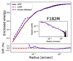
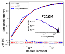
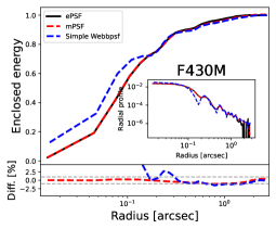
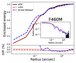
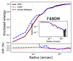
Figure 13: Similar to Figure 12, but for the 5 medium-band NIRCam filters used by JEMS.

Appendix B SED fitting with different priors of star formation history

Apart from the fiducial SED fitting with nonparametric SFHs assuming the continuity prior (Section 2.4), we have also tested our Prospector fitting results using the other two SFHs, namely, nonparametric SFHs with the Dirichlet prior (Leja et al., 2017) and parametric SFHs with a delayed-tau functional form. For the difference between the continuity and Dirichlet priors, we refer readers to Leja et al. (2017) for details. In short, these two priors for nonparametric SFHs are very similar except that the continuity prior is strongly against sudden changes in star formation rate in adjacent lookback time bins. For the delayed-tau model, i.e. $\rm{SFR}(t)\propto(t-t_{age})e^{-(t-t_{age})/\tau}$, we fit $\tau$ with a logarithmically flat prior of $\log(\tau/\rm{Gyr})\in(-2,1)$, and $t_{\rm{age}}$ with a flat prior of $t_{\rm{age}}/\rm{Gyr}\in(10^{-3},t_{\rm{H}})$.

In Figure 14, we compare the measurements of stellar mass and star formation rate from different SFH assumptions. Very good agreement is seen across the three SFH models. In Figure 15 and 16, we compare the fiducial reconstructed SFHs with the delayed-tau and Dirichlet nonparametric SFHs, respectively. As expected, the nonparamtric SFHs are able to capture more complex shapes than the delayed-tau ones, but the overall shapes of these two SFHs are very similar. Meanwhile, relative to the fiducial SFHs from the continuity prior, the Dirichlet nonparametric SFHs show larger fluctuations in star formation rate in adjacent lookback time bins, but these two nonparametric SFHs are in general mirror each other in terms of their overall shapes. The tests here show that the results of this work are not sensitive to the assumptions of SED models.

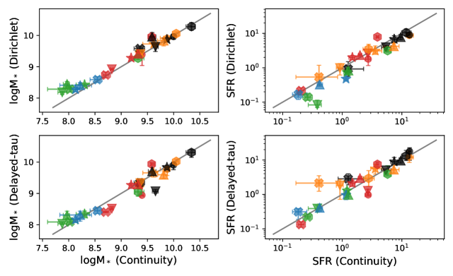
Figure 14: Comparisons of stellar-mass and star formation rate measures from different SFHs for the individual structural components of the 6 galaxies presented in this work. Color-coding is the same as Figure 5 in the main text (C1 are in red). Symbols used for individual galaxies are the same as Figure 8 in the main text. The black solid line in each panel marks the one-to-one relationship.

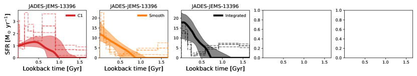
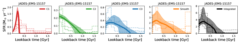
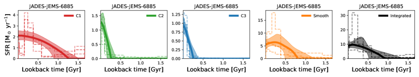
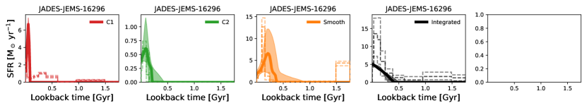
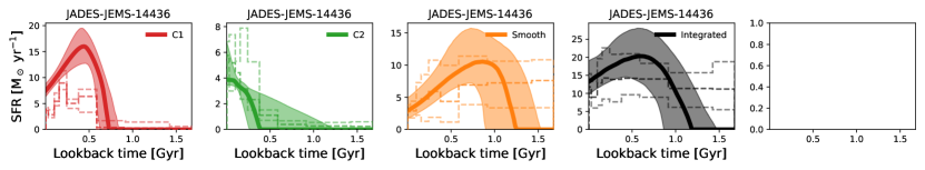
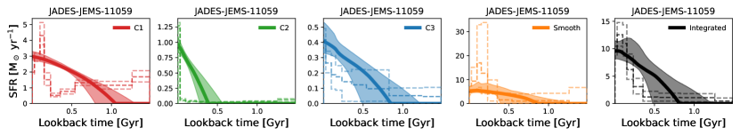
Figure 15: The comparison of the nonparametric SFH reconstructed by our fiducial model (Section 2.4), plotted as dashed lines, with the SFH derived from a parametric delayed-tau model, plotted as solid lines (the best-fit) and shaded regions (1$\sigma$ uncertainty).

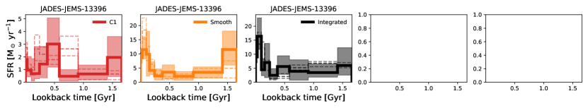
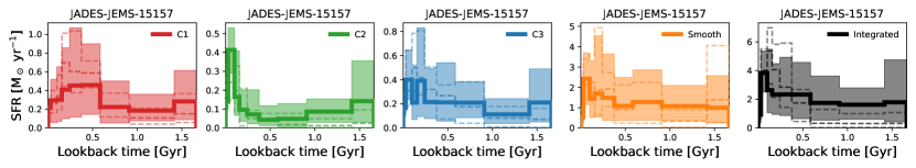
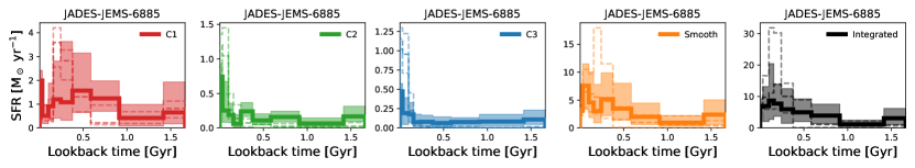
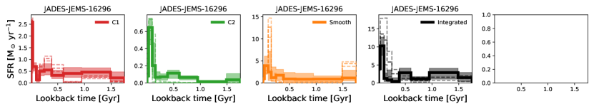
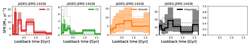
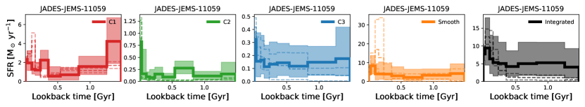
Figure 16: Similar to Figure 15, but now comparing with the nonparametric SFH reconstructed using the Dirichlet prior.

Appendix C Detailed descriptions of the spatially resolved stellar populations of the 6 galaxies

JADES-JEMS-13396. The top row of Figure 5 shows the SED fitting result of this galaxy. Despite that the mass-weighted stellar age of C1 is consistent with that of the Smooth component, the shapes of their SFHs are different. For the Smooth component, its mass assembly was at a relatively low, but non-negligible rate in early times of $t_{\rm{lookback}}>0.4$ Gyr, followed by a rapid increase in SFR. For C1, however, its most mass formed through a recent star-formation episode during $t_{\rm{lookback}}=0.2\sim 0.8$ Gyr. By the time of observation, the Smooth component is forming stars at a higher rate than C1, with the sSFR of the former being $\approx$ 1.6 times larger (Table 2). These differences in SFH shapes qualitatively remains if we instead use a parametric delayed-tau or nonparametric Dirichlet SFH priors (Figure 15 and 16). We also notice that a color gradient is clearly present in the Smooth component, with the upper-left side (likely contains several faint clumps in it) being bluer than its rest parts.

JADES-JEMS-15157. The middle row of Figure 5 shows the SED fitting result of this galaxy. Unlike C2 having a monotonically rising SFH, the SFH of C1 gradually rises toward a relatively recent peak at $t_{\rm{lookback}}$ $\approx 0.3$ Gyr, followed by a rapid decline over the past 0.2 Gyr. By the time of observation, the sSFR of C1 is only $\approx 0.4$ Gyr^-1, $\approx$ 7.5 times smaller than that of C2 (Table 2). We note that C3 has a similar stellar population to that of C1, but this is because the spatial separation between C1 and C3 is so small – about 0.1” that is smaller than the angular resolution of NIRCam/F444W imaging – that the aperture photometry (Section 2.3) for one substructure is significantly affected by the other. Finally, while C1 and the Smooth component share a similar SFH in early times, they differentiate from each other at late times: unlike C1 whose SFR quickly declined after the $t_{\rm{lookback}}$ $\approx 0.3$ Gyr peak, the Smooth component retained that peak SFR toward a later time of $t_{\rm{lookback}}$ $<0.1$ Gyr. All these remain qualitatively unchanged if we instead use a parametric delayed-tau or nonparametric Dirichlet SFH priors (Figure 15 and 16).

JADES-JEMS-6885. The bottom row of Figure 5 shows the SED fitting result of this galaxy. There is no significant mass assembly before $t_{\rm{lookback}}$ $>1$ Gyr for all structural components, but their SFHs are different over the recent 1 Gyr. Compared to C2 and C3, C1 is older by $0.3\sim 0.5$ Gyr (Table 2). Moreover, C1 has a poststarburst-like SFH, namely, it experienced a burst of star formation during $t_{\rm{lookback}}$ $=0.2\sim 0.6$ Gyr, followed by a rapid decline of SFR. Differing from C1, C2 and C3 are experiencing on-going bursts of star formation started $\approx$ 0.2 Gyr ago. By the time of observation, the sSFR of C1 is 6.3 and 9.3 times smaller than that of C2 and C3, respectively. Finally, while the Smooth component generally mirrored the shape of C1’s SFH before the peak ($t_{\rm{lookback}}$ $\approx 0.2$ Gyr), they differed from each other afterward: the SFR of C1 quickly declined to a very low level, while the Smooth component retained the peak SFR to a later time of $t_{\rm{lookback}}$ $<0.1$ Gyr. All these differences in the SFHs of different structural components remain qualitatively unchanged if we instead use the other two SFH priors (Figure 15 and 16).

JADES-JEMS-16296. The top row of Figure 6 shows the SED fitting result of this galaxy. Both C1 and C2 are experiencing bursts of star formation started $\lesssim 0.1$ Gyr ago, and their instantaneous sSFRs are similar, $\approx 5$ Gyr^-1. While it is not seen from the delayed-tau SFH (Figure 15), the reconstructed nonparametric SFH (Figure 6 and 16) suggests that older ($t_{\rm{lookback}}$ $\gtrsim 0.5$ Gyr) stellar populations are also present in C1, leading to its larger mass-weighted stellar age than C2 (Table 2).

JADES-JEMS-14436. The middle row of Figure 6 shows the SED fitting result of this galaxy. The major mass assembly event of C1 started at $t_{\rm{lookback}}$ $\approx 0.6$ Gyr, peaked at $t_{\rm{lookback}}$ $\approx 0.2$ Gyr and gradually declined afterward. For C2, its SFR monotonically increased since $t_{\rm{lookback}}$ $\approx 0.8$ Gyr, before which its SFR was consistent with zero. There also seems to be a tidal tail associated with C2 (see e.g. NIRCam F150W cutouts in Figure 3), so this is a possible merging system. Also noticed for this galaxy is that the Smooth component has a very extended SFH, namely, its mass assembly began at $t_{\rm{lookback}}$ $>1$ Gyr, corresponding to redshift $z>7$, and the SFR started to decline since $t_{\rm{lookback}}$ $\approx 0.6$ Gyr. All these features in SFHs remain qualitatively unchanged if we instead use the other two SFH priors (Figure 15 and 16).

JADES-JEMS-11059. The bottom row of Figure 6 shows the SED fitting result of this galaxy. C1 contains old stellar populations with age $>1$ Gyr, and it also has a recent burst of star formation that started $\approx 0.2$ Gyr ago, peaked at $t_{\rm{lookback}}$ $\approx 0.1$ Gyr and declined afterward. Meanwhile, C3 has an overall rising SFH. For C2, although it is not in the segmentation map of the galaxy (Figure 3), it is still included to the analysis because its photometric redshift solution is consistent with that of the galaxy JADES-JEMS-11059. C2 is experiencing a starburst started $\lesssim 0.3$ Gyr ago.

References

- Anderson & King (2000) Anderson, J., & King, I. R. 2000, PASP, 112, 1360, doi: 10.1086/316632
- Athanassoula et al. (2015) Athanassoula, E., Laurikainen, E., Salo, H., & Bosma, A. 2015, MNRAS, 454, 3843, doi: 10.1093/mnras/stv2231
- Bacon et al. (2022) Bacon, R., Brinchmann, J., Conseil, S., et al. 2022, arXiv e-prints, arXiv:2211.08493. https://arxiv.org/abs/2211.08493
- Balogh et al. (1999) Balogh, M. L., Morris, S. L., Yee, H. K. C., Carlberg, R. G., & Ellingson, E. 1999, ApJ, 527, 54, doi: 10.1086/30805610.48550/arXiv.astro-ph/9906470
- Barbuy et al. (2018) Barbuy, B., Chiappini, C., & Gerhard, O. 2018, ARA&A, 56, 223, doi: 10.1146/annurev-astro-081817-051826
- Barnes & Hernquist (1996) Barnes, J. E., & Hernquist, L. 1996, ApJ, 471, 115, doi: 10.1086/177957
- Barro et al. (2017) Barro, G., Faber, S. M., Koo, D. C., et al. 2017, ApJ, 840, 47, doi: 10.3847/1538-4357/aa6b05
- Behrendt et al. (2015) Behrendt, M., Burkert, A., & Schartmann, M. 2015, MNRAS, 448, 1007, doi: 10.1093/mnras/stv027
- Behroozi et al. (2013a) Behroozi, P. S., Wechsler, R. H., & Conroy, C. 2013a, ApJ, 770, 57, doi: 10.1088/0004-637X/770/1/57
- Behroozi et al. (2013b) —. 2013b, ApJ, 762, L31, doi: 10.1088/2041-8205/762/2/L31
- Belli et al. (2015) Belli, S., Newman, A. B., & Ellis, R. S. 2015, ApJ, 799, 206, doi: 10.1088/0004-637X/799/2/206
- Binney & Tremaine (2008) Binney, J., & Tremaine, S. 2008, Galactic Dynamics: Second Edition
- Boucaud et al. (2016) Boucaud, A., Bocchio, M., Abergel, A., et al. 2016, A&A, 596, A63, doi: 10.1051/0004-6361/201629080
- Bournaud (2016) Bournaud, F. 2016, in Astrophysics and Space Science Library, Vol. 418, Galactic Bulges, ed. E. Laurikainen, R. Peletier, & D. Gadotti, 355, doi: 10.1007/978-3-319-19378-6_13
- Bournaud et al. (2007) Bournaud, F., Elmegreen, B. G., & Elmegreen, D. M. 2007, ApJ, 670, 237, doi: 10.1086/522077
- Bournaud et al. (2005) Bournaud, F., Jog, C. J., & Combes, F. 2005, A&A, 437, 69, doi: 10.1051/0004-6361:20042036
- Bournaud et al. (2014) Bournaud, F., Perret, V., Renaud, F., et al. 2014, ApJ, 780, 57, doi: 10.1088/0004-637X/780/1/57
- Bradley et al. (2022) Bradley, L., Sipőcz, B., Robitaille, T., et al. 2022, astropy/photutils: 1.5.0, 1.5.0, Zenodo, doi: 10.5281/zenodo.6825092
- Brinchmann et al. (2004) Brinchmann, J., Charlot, S., White, S. D. M., et al. 2004, MNRAS, 351, 1151, doi: 10.1111/j.1365-2966.2004.07881.x
- Bruce et al. (2012) Bruce, V. A., Dunlop, J. S., Cirasuolo, M., et al. 2012, MNRAS, 427, 1666, doi: 10.1111/j.1365-2966.2012.22087.x
- Bruce et al. (2014) Bruce, V. A., Dunlop, J. S., McLure, R. J., et al. 2014, MNRAS, 444, 1001, doi: 10.1093/mnras/stu1478
- Bruzual A. (1983) Bruzual A., G. 1983, ApJ, 273, 105, doi: 10.1086/161352
- Buck et al. (2017) Buck, T., Macciò, A. V., Obreja, A., et al. 2017, MNRAS, 468, 3628, doi: 10.1093/mnras/stx685
- Bundy et al. (2010) Bundy, K., Scarlata, C., Carollo, C. M., et al. 2010, ApJ, 719, 1969, doi: 10.1088/0004-637X/719/2/1969
- Byler et al. (2017) Byler, N., Dalcanton, J. J., Conroy, C., & Johnson, B. D. 2017, ApJ, 840, 44, doi: 10.3847/1538-4357/aa6c66
- Calzetti et al. (2000) Calzetti, D., Armus, L., Bohlin, R. C., et al. 2000, ApJ, 533, 682, doi: 10.1086/308692
- Carnall et al. (2019a) Carnall, A. C., Leja, J., Johnson, B. D., et al. 2019a, ApJ, 873, 44, doi: 10.3847/1538-4357/ab04a2
- Carnall et al. (2019b) Carnall, A. C., McLure, R. J., Dunlop, J. S., et al. 2019b, MNRAS, 490, 417, doi: 10.1093/mnras/stz2544
- Carnall et al. (2023a) Carnall, A. C., McLeod, D. J., McLure, R. J., et al. 2023a, MNRAS, doi: 10.1093/mnras/stad369
- Carnall et al. (2023b) Carnall, A. C., McLure, R. J., Dunlop, J. S., et al. 2023b, arXiv e-prints, arXiv:2301.11413, doi: 10.48550/arXiv.2301.11413
- Catinella et al. (2013) Catinella, B., Schiminovich, D., Cortese, L., et al. 2013, MNRAS, 436, 34, doi: 10.1093/mnras/stt1417
- Ceverino et al. (2010) Ceverino, D., Dekel, A., & Bournaud, F. 2010, MNRAS, 404, 2151, doi: 10.1111/j.1365-2966.2010.16433.x
- Ceverino et al. (2012) Ceverino, D., Dekel, A., Mandelker, N., et al. 2012, MNRAS, 420, 3490, doi: 10.1111/j.1365-2966.2011.20296.x
- Ceverino et al. (2014) Ceverino, D., Klypin, A., Klimek, E. S., et al. 2014, MNRAS, 442, 1545, doi: 10.1093/mnras/stu956
- Charlot & Fall (2000) Charlot, S., & Fall, S. M. 2000, ApJ, 539, 718, doi: 10.1086/309250
- Cheung et al. (2012) Cheung, E., Faber, S. M., Koo, D. C., et al. 2012, ApJ, 760, 131, doi: 10.1088/0004-637X/760/2/131
- Choi et al. (2016) Choi, J., Dotter, A., Conroy, C., et al. 2016, ApJ, 823, 102, doi: 10.3847/0004-637X/823/2/102
- Conroy & Gunn (2010) Conroy, C., & Gunn, J. E. 2010, ApJ, 712, 833, doi: 10.1088/0004-637X/712/2/833
- Conroy et al. (2009) Conroy, C., Gunn, J. E., & White, M. 2009, ApJ, 699, 486, doi: 10.1088/0004-637X/699/1/486
- Conselice et al. (2000) Conselice, C. J., Bershady, M. A., & Jangren, A. 2000, ApJ, 529, 886, doi: 10.1086/308300
- Cowie et al. (1995) Cowie, L. L., Hu, E. M., & Songaila, A. 1995, AJ, 110, 1576, doi: 10.1086/117631
- Daddi et al. (2010) Daddi, E., Bournaud, F., Walter, F., et al. 2010, ApJ, 713, 686, doi: 10.1088/0004-637X/713/1/686
- Debattista et al. (2004) Debattista, V. P., Carollo, C. M., Mayer, L., & Moore, B. 2004, ApJ, 604, L93, doi: 10.1086/386332
- Dekel & Burkert (2014) Dekel, A., & Burkert, A. 2014, MNRAS, 438, 1870, doi: 10.1093/mnras/stt2331
- Dekel & Krumholz (2013) Dekel, A., & Krumholz, M. R. 2013, MNRAS, 432, 455, doi: 10.1093/mnras/stt480
- Dekel et al. (2009) Dekel, A., Sari, R., & Ceverino, D. 2009, ApJ, 703, 785, doi: 10.1088/0004-637X/703/1/785
- Dessauges-Zavadsky & Adamo (2018) Dessauges-Zavadsky, M., & Adamo, A. 2018, MNRAS, 479, L118, doi: 10.1093/mnrasl/sly112
- Dimauro et al. (2022) Dimauro, P., Daddi, E., Shankar, F., et al. 2022, MNRAS, 513, 256, doi: 10.1093/mnras/stac884
- Dotter (2016) Dotter, A. 2016, ApJS, 222, 8, doi: 10.3847/0067-0049/222/1/8
- Eisenstein et al. (2017) Eisenstein, D. J., Ferruit, P., Rieke, M. J., Willmer, C. N. A., & Willott, C. J. 2017, NIRCam-NIRSpec galaxy assembly survey - GOODS-S - part #1a, JWST Proposal. Cycle 1, ID. #1180
- Eliche-Moral et al. (2011) Eliche-Moral, M. C., González-García, A. C., Balcells, M., et al. 2011, A&A, 533, A104, doi: 10.1051/0004-6361/201116509
- Elmegreen et al. (2008) Elmegreen, B. G., Bournaud, F., & Elmegreen, D. M. 2008, ApJ, 688, 67, doi: 10.1086/592190
- Elmegreen & Elmegreen (2005) Elmegreen, B. G., & Elmegreen, D. M. 2005, ApJ, 627, 632, doi: 10.1086/430514
- Elmegreen et al. (2009) Elmegreen, D. M., Elmegreen, B. G., Marcus, M. T., et al. 2009, ApJ, 701, 306, doi: 10.1088/0004-637X/701/1/306
- Elmegreen et al. (2007) Elmegreen, D. M., Elmegreen, B. G., Ravindranath, S., & Coe, D. A. 2007, ApJ, 658, 763, doi: 10.1086/511667
- Escala & Larson (2008) Escala, A., & Larson, R. B. 2008, ApJ, 685, L31, doi: 10.1086/592271
- Estrada-Carpenter et al. (2020) Estrada-Carpenter, V., Papovich, C., Momcheva, I., et al. 2020, ApJ, 898, 171, doi: 10.3847/1538-4357/aba004
- Falcón-Barroso et al. (2011) Falcón-Barroso, J., Sánchez-Blázquez, P., Vazdekis, A., et al. 2011, A&A, 532, A95, doi: 10.1051/0004-6361/201116842
- Fang et al. (2013) Fang, J. J., Faber, S. M., Koo, D. C., & Dekel, A. 2013, ApJ, 776, 63, doi: 10.1088/0004-637X/776/1/63
- Ferguson et al. (2004) Ferguson, H. C., Dickinson, M., Giavalisco, M., et al. 2004, ApJ, 600, L107, doi: 10.1086/378578
- Förster Schreiber & Wuyts (2020) Förster Schreiber, N. M., & Wuyts, S. 2020, ARA&A, 58, 661, doi: 10.1146/annurev-astro-032620-021910
- Förster Schreiber et al. (2006) Förster Schreiber, N. M., Genzel, R., Lehnert, M. D., et al. 2006, ApJ, 645, 1062, doi: 10.1086/504403
- Förster Schreiber et al. (2009) Förster Schreiber, N. M., Genzel, R., Bouché, N., et al. 2009, ApJ, 706, 1364, doi: 10.1088/0004-637X/706/2/1364
- Förster Schreiber et al. (2011) Förster Schreiber, N. M., Shapley, A. E., Genzel, R., et al. 2011, ApJ, 739, 45, doi: 10.1088/0004-637X/739/1/45
- Förster Schreiber et al. (2018) Förster Schreiber, N. M., Renzini, A., Mancini, C., et al. 2018, ApJS, 238, 21, doi: 10.3847/1538-4365/aadd49
- Franx et al. (2008) Franx, M., van Dokkum, P. G., Förster Schreiber, N. M., et al. 2008, ApJ, 688, 770, doi: 10.1086/592431
- Gaia Collaboration et al. (2021) Gaia Collaboration, Brown, A. G. A., Vallenari, A., et al. 2021, A&A, 649, A1, doi: 10.1051/0004-6361/202039657
- Gardner et al. (2023) Gardner, J. P., Mather, J. C., Abbott, R., et al. 2023, arXiv e-prints, arXiv:2304.04869, doi: 10.48550/arXiv.2304.04869
- Genel et al. (2012) Genel, S., Naab, T., Genzel, R., et al. 2012, ApJ, 745, 11, doi: 10.1088/0004-637X/745/1/11
- Genzel et al. (2006) Genzel, R., Tacconi, L. J., Eisenhauer, F., et al. 2006, Nature, 442, 786, doi: 10.1038/nature05052
- Genzel et al. (2008) Genzel, R., Burkert, A., Bouché, N., et al. 2008, ApJ, 687, 59, doi: 10.1086/591840
- Genzel et al. (2011) Genzel, R., Newman, S., Jones, T., et al. 2011, ApJ, 733, 101, doi: 10.1088/0004-637X/733/2/101
- Genzel et al. (2015) Genzel, R., Tacconi, L. J., Lutz, D., et al. 2015, ApJ, 800, 20, doi: 10.1088/0004-637X/800/1/20
- Genzel et al. (2020) Genzel, R., Price, S. H., Übler, H., et al. 2020, ApJ, 902, 98, doi: 10.3847/1538-4357/abb0ea
- Giavalisco et al. (2004) Giavalisco, M., Ferguson, H. C., Koekemoer, A. M., et al. 2004, ApJ, 600, L93, doi: 10.1086/379232
- Grogin et al. (2011) Grogin, N. A., Kocevski, D. D., Faber, S. M., et al. 2011, ApJS, 197, 35, doi: 10.1088/0067-0049/197/2/35
- Guedes et al. (2013) Guedes, J., Mayer, L., Carollo, M., & Madau, P. 2013, ApJ, 772, 36, doi: 10.1088/0004-637X/772/1/36
- Guo et al. (2012) Guo, Y., Giavalisco, M., Ferguson, H. C., Cassata, P., & Koekemoer, A. M. 2012, ApJ, 757, 120, doi: 10.1088/0004-637X/757/2/120
- Guo et al. (2015) Guo, Y., Ferguson, H. C., Bell, E. F., et al. 2015, ApJ, 800, 39, doi: 10.1088/0004-637X/800/1/39
- Guo et al. (2018) Guo, Y., Rafelski, M., Bell, E. F., et al. 2018, ApJ, 853, 108, doi: 10.3847/1538-4357/aaa018
- Hasselquist et al. (2020) Hasselquist, S., Zasowski, G., Feuillet, D. K., et al. 2020, ApJ, 901, 109, doi: 10.3847/1538-4357/abaeee
- Hernquist (1989) Hernquist, L. 1989, Nature, 340, 687, doi: 10.1038/340687a0
- Hopkins et al. (2009) Hopkins, P. F., Cox, T. J., Younger, J. D., & Hernquist, L. 2009, ApJ, 691, 1168, doi: 10.1088/0004-637X/691/2/1168
- Hopkins et al. (2012) Hopkins, P. F., Kereš, D., Murray, N., Quataert, E., & Hernquist, L. 2012, MNRAS, 427, 968, doi: 10.1111/j.1365-2966.2012.21981.x
- Huertas-Company et al. (2015) Huertas-Company, M., Gravet, R., Cabrera-Vives, G., et al. 2015, ApJS, 221, 8, doi: 10.1088/0067-0049/221/1/8
- Huertas-Company et al. (2020) Huertas-Company, M., Guo, Y., Ginzburg, O., et al. 2020, MNRAS, 499, 814, doi: 10.1093/mnras/staa2777
- Ilbert et al. (2010) Ilbert, O., Salvato, M., Le Floc’h, E., et al. 2010, ApJ, 709, 644, doi: 10.1088/0004-637X/709/2/644
- Ilbert et al. (2013) Ilbert, O., McCracken, H. J., Le Fèvre, O., et al. 2013, A&A, 556, A55, doi: 10.1051/0004-6361/201321100
- Illingworth et al. (2016) Illingworth, G., Magee, D., Bouwens, R., et al. 2016, arXiv e-prints, arXiv:1606.00841. https://arxiv.org/abs/1606.00841
- Immeli et al. (2004) Immeli, A., Samland, M., Westera, P., & Gerhard, O. 2004, ApJ, 611, 20, doi: 10.1086/422179
- Inoue et al. (2016) Inoue, S., Dekel, A., Mandelker, N., et al. 2016, MNRAS, 456, 2052, doi: 10.1093/mnras/stv2793
- Inoue & Saitoh (2012) Inoue, S., & Saitoh, T. R. 2012, MNRAS, 422, 1902, doi: 10.1111/j.1365-2966.2011.20338.x
- Ji & Giavalisco (2022) Ji, Z., & Giavalisco, M. 2022, ApJ, 935, 120, doi: 10.3847/1538-4357/ac7f43
- Ji & Giavalisco (2023) —. 2023, ApJ, 943, 54, doi: 10.3847/1538-4357/aca807
- Ji et al. (2022) Ji, Z., Giavalisco, M., Kirkpatrick, A., et al. 2022, ApJ, 925, 74, doi: 10.3847/1538-4357/ac3837
- Ji et al. (2018) Ji, Z., Giavalisco, M., Williams, C. C., et al. 2018, ApJ, 862, 135, doi: 10.3847/1538-4357/aacc2c
- Johnson et al. (2021) Johnson, B. D., Leja, J., Conroy, C., & Speagle, J. S. 2021, ApJS, 254, 22, doi: 10.3847/1538-4365/abef67
- Kassin et al. (2012) Kassin, S. A., Weiner, B. J., Faber, S. M., et al. 2012, ApJ, 758, 106, doi: 10.1088/0004-637X/758/2/106
- Kauffmann et al. (2003) Kauffmann, G., Heckman, T. M., White, S. D. M., et al. 2003, MNRAS, 341, 33, doi: 10.1046/j.1365-8711.2003.06291.x
- Koekemoer et al. (2011) Koekemoer, A. M., Faber, S. M., Ferguson, H. C., et al. 2011, ApJS, 197, 36, doi: 10.1088/0067-0049/197/2/36
- Kormendy & Kennicutt (2004) Kormendy, J., & Kennicutt, Robert C., J. 2004, ARA&A, 42, 603, doi: 10.1146/annurev.astro.42.053102.134024
- Kriek & Conroy (2013) Kriek, M., & Conroy, C. 2013, ApJ, 775, L16, doi: 10.1088/2041-8205/775/1/L16
- Kroupa (2001) Kroupa, P. 2001, MNRAS, 322, 231, doi: 10.1046/j.1365-8711.2001.04022.x
- Labbé et al. (2005) Labbé, I., Huang, J., Franx, M., et al. 2005, ApJ, 624, L81, doi: 10.1086/430700
- Lang et al. (2014) Lang, P., Wuyts, S., Somerville, R. S., et al. 2014, ApJ, 788, 11, doi: 10.1088/0004-637X/788/1/11
- Law et al. (2009) Law, D. R., Steidel, C. C., Erb, D. K., et al. 2009, ApJ, 697, 2057, doi: 10.1088/0004-637X/697/2/2057
- Leja et al. (2019) Leja, J., Carnall, A. C., Johnson, B. D., Conroy, C., & Speagle, J. S. 2019, ApJ, 876, 3, doi: 10.3847/1538-4357/ab133c
- Leja et al. (2017) Leja, J., Johnson, B. D., Conroy, C., van Dokkum, P. G., & Byler, N. 2017, ApJ, 837, 170, doi: 10.3847/1538-4357/aa5ffe
- Leja et al. (2022) Leja, J., Speagle, J. S., Ting, Y.-S., et al. 2022, ApJ, 936, 165, doi: 10.3847/1538-4357/ac887d
- Liu et al. (2019) Liu, D., Schinnerer, E., Groves, B., et al. 2019, ApJ, 887, 235, doi: 10.3847/1538-4357/ab578d
- Lotz et al. (2004) Lotz, J. M., Primack, J., & Madau, P. 2004, AJ, 128, 163, doi: 10.1086/421849
- Lotz et al. (2017) Lotz, J. M., Koekemoer, A., Coe, D., et al. 2017, ApJ, 837, 97, doi: 10.3847/1538-4357/837/1/97
- Luo et al. (2017) Luo, B., Brandt, W. N., Xue, Y. Q., et al. 2017, ApJS, 228, 2, doi: 10.3847/1538-4365/228/1/2
- Lyu et al. (2022) Lyu, J., Alberts, S., Rieke, G. H., & Rujopakarn, W. 2022, arXiv e-prints, arXiv:2209.06219. https://arxiv.org/abs/2209.06219
- Madau (1995) Madau, P. 1995, ApJ, 441, 18, doi: 10.1086/175332
- Mandelker et al. (2017) Mandelker, N., Dekel, A., Ceverino, D., et al. 2017, MNRAS, 464, 635, doi: 10.1093/mnras/stw2358
- Mandelker et al. (2014) —. 2014, MNRAS, 443, 3675, doi: 10.1093/mnras/stu1340
- McGaugh & Schombert (2014) McGaugh, S. S., & Schombert, J. M. 2014, AJ, 148, 77, doi: 10.1088/0004-6256/148/5/77
- Merlin et al. (2019) Merlin, E., Fortuni, F., Torelli, M., et al. 2019, MNRAS, 490, 3309, doi: 10.1093/mnras/stz2615
- Merlin et al. (2021) Merlin, E., Castellano, M., Santini, P., et al. 2021, A&A, 649, A22, doi: 10.1051/0004-6361/202140310
- Mosleh et al. (2017) Mosleh, M., Tacchella, S., Renzini, A., et al. 2017, ApJ, 837, 2, doi: 10.3847/1538-4357/aa5f14
- Murata et al. (2014) Murata, K. L., Kajisawa, M., Taniguchi, Y., et al. 2014, ApJ, 786, 15, doi: 10.1088/0004-637X/786/1/15
- Murray et al. (2010) Murray, N., Quataert, E., & Thompson, T. A. 2010, ApJ, 709, 191, doi: 10.1088/0004-637X/709/1/191
- Muzzin et al. (2013) Muzzin, A., Marchesini, D., Stefanon, M., et al. 2013, ApJ, 777, 18, doi: 10.1088/0004-637X/777/1/18
- Nelson et al. (2014) Nelson, E., van Dokkum, P., Franx, M., et al. 2014, Nature, 513, 394, doi: 10.1038/nature13616
- Nenkova et al. (2008a) Nenkova, M., Sirocky, M. M., Ivezić, Ž., & Elitzur, M. 2008a, ApJ, 685, 147, doi: 10.1086/590482
- Nenkova et al. (2008b) Nenkova, M., Sirocky, M. M., Nikutta, R., Ivezić, Ž., & Elitzur, M. 2008b, ApJ, 685, 160, doi: 10.1086/590483
- Newman et al. (2015) Newman, A. B., Belli, S., & Ellis, R. S. 2015, ApJ, 813, L7, doi: 10.1088/2041-8205/813/1/L7
- Newman et al. (2018) Newman, A. B., Belli, S., Ellis, R. S., & Patel, S. G. 2018, ApJ, 862, 126, doi: 10.3847/1538-4357/aacd4f
- Noguchi (1999) Noguchi, M. 1999, ApJ, 514, 77, doi: 10.1086/306932
- Noll et al. (2009) Noll, S., Burgarella, D., Giovannoli, E., et al. 2009, A&A, 507, 1793, doi: 10.1051/0004-6361/200912497
- Oesch et al. (2023) Oesch, P. A., Brammer, G., Naidu, R. P., et al. 2023, arXiv e-prints, arXiv:2304.02026, doi: 10.48550/arXiv.2304.02026
- Okamoto (2013) Okamoto, T. 2013, MNRAS, 428, 718, doi: 10.1093/mnras/sts067
- Perez et al. (2013) Perez, J., Valenzuela, O., Tissera, P. B., & Michel-Dansac, L. 2013, MNRAS, 436, 259, doi: 10.1093/mnras/stt1563
- Péroux & Howk (2020) Péroux, C., & Howk, J. C. 2020, ARA&A, 58, 363, doi: 10.1146/annurev-astro-021820-120014
- Perret et al. (2014) Perret, V., Renaud, F., Epinat, B., et al. 2014, A&A, 562, A1, doi: 10.1051/0004-6361/201322395
- Perrin et al. (2014) Perrin, M. D., Sivaramakrishnan, A., Lajoie, C.-P., et al. 2014, in Society of Photo-Optical Instrumentation Engineers (SPIE) Conference Series, Vol. 9143, Space Telescopes and Instrumentation 2014: Optical, Infrared, and Millimeter Wave, ed. J. Oschmann, Jacobus M., M. Clampin, G. G. Fazio, & H. A. MacEwen, 91433X, doi: 10.1117/12.2056689
- Perrin et al. (2012) Perrin, M. D., Soummer, R., Elliott, E. M., Lallo, M. D., & Sivaramakrishnan, A. 2012, in Society of Photo-Optical Instrumentation Engineers (SPIE) Conference Series, Vol. 8442, Space Telescopes and Instrumentation 2012: Optical, Infrared, and Millimeter Wave, ed. M. C. Clampin, G. G. Fazio, H. A. MacEwen, & J. Oschmann, Jacobus M., 84423D, doi: 10.1117/12.925230
- Pillepich et al. (2019) Pillepich, A., Nelson, D., Springel, V., et al. 2019, MNRAS, 490, 3196, doi: 10.1093/mnras/stz2338
- Planck Collaboration et al. (2020) Planck Collaboration, Aghanim, N., Akrami, Y., et al. 2020, A&A, 641, A6, doi: 10.1051/0004-6361/201833910
- Popesso et al. (2023) Popesso, P., Concas, A., Cresci, G., et al. 2023, MNRAS, 519, 1526, doi: 10.1093/mnras/stac3214
- Posti & Helmi (2019) Posti, L., & Helmi, A. 2019, A&A, 621, A56, doi: 10.1051/0004-6361/201833355
- Prochaska & Wolfe (2009) Prochaska, J. X., & Wolfe, A. M. 2009, ApJ, 696, 1543, doi: 10.1088/0004-637X/696/2/1543
- Quadri et al. (2007) Quadri, R., Marchesini, D., van Dokkum, P., et al. 2007, AJ, 134, 1103, doi: 10.1086/520330
- Rao et al. (2006) Rao, S. M., Turnshek, D. A., & Nestor, D. B. 2006, ApJ, 636, 610, doi: 10.1086/498132
- Rieke et al. (2023) Rieke, M. J., Kelly, D. M., Misselt, K., et al. 2023, PASP, 135, 028001, doi: 10.1088/1538-3873/acac53
- Robertson et al. (2022) Robertson, B. E., Tacchella, S., Johnson, B. D., et al. 2022, arXiv e-prints, arXiv:2212.04480. https://arxiv.org/abs/2212.04480
- Saintonge et al. (2011) Saintonge, A., Kauffmann, G., Kramer, C., et al. 2011, MNRAS, 415, 32, doi: 10.1111/j.1365-2966.2011.18677.x
- Santini et al. (2022) Santini, P., Castellano, M., Fontana, A., et al. 2022, ApJ, 940, 135, doi: 10.3847/1538-4357/ac9a48
- Sattari et al. (2023) Sattari, Z., Mobasher, B., Chartab, N., et al. 2023, arXiv e-prints, arXiv:2305.09021, doi: 10.48550/arXiv.2305.09021
- Schreiber et al. (2018) Schreiber, C., Glazebrook, K., Nanayakkara, T., et al. 2018, A&A, 618, A85, doi: 10.1051/0004-6361/201833070
- Scoville et al. (2017) Scoville, N., Lee, N., Vanden Bout, P., et al. 2017, ApJ, 837, 150, doi: 10.3847/1538-4357/aa61a0
- Shahidi et al. (2020) Shahidi, A., Mobasher, B., Nayyeri, H., et al. 2020, ApJ, 897, 44, doi: 10.3847/1538-4357/ab96c5
- Shapiro et al. (2008) Shapiro, K. L., Genzel, R., Förster Schreiber, N. M., et al. 2008, ApJ, 682, 231, doi: 10.1086/587133
- Shibuya et al. (2015) Shibuya, T., Ouchi, M., & Harikane, Y. 2015, ApJS, 219, 15, doi: 10.1088/0067-0049/219/2/15
- Shibuya et al. (2016) Shibuya, T., Ouchi, M., Kubo, M., & Harikane, Y. 2016, ApJ, 821, 72, doi: 10.3847/0004-637X/821/2/72
- Simons et al. (2017) Simons, R. C., Kassin, S. A., Weiner, B. J., et al. 2017, ApJ, 843, 46, doi: 10.3847/1538-4357/aa740c
- Skilling (2004) Skilling, J. 2004, in American Institute of Physics Conference Series, Vol. 735, Bayesian Inference and Maximum Entropy Methods in Science and Engineering: 24th International Workshop on Bayesian Inference and Maximum Entropy Methods in Science and Engineering, ed. R. Fischer, R. Preuss, & U. V. Toussaint, 395–405, doi: 10.1063/1.1835238
- Soto et al. (2017) Soto, E., de Mello, D. F., Rafelski, M., et al. 2017, ApJ, 837, 6, doi: 10.3847/1538-4357/aa5da3
- Speagle (2020) Speagle, J. S. 2020, MNRAS, 493, 3132, doi: 10.1093/mnras/staa278
- Suess et al. (2021) Suess, K. A., Kriek, M., Price, S. H., & Barro, G. 2021, ApJ, 915, 87, doi: 10.3847/1538-4357/abf1e4
- Suess et al. (2022) Suess, K. A., Leja, J., Johnson, B. D., et al. 2022, ApJ, 935, 146, doi: 10.3847/1538-4357/ac82b0
- Tacchella et al. (2016) Tacchella, S., Dekel, A., Carollo, C. M., et al. 2016, MNRAS, 458, 242, doi: 10.1093/mnras/stw303
- Tacchella et al. (2015) Tacchella, S., Carollo, C. M., Renzini, A., et al. 2015, Science, 348, 314, doi: 10.1126/science.1261094
- Tacchella et al. (2018) Tacchella, S., Carollo, C. M., Förster Schreiber, N. M., et al. 2018, ApJ, 859, 56, doi: 10.3847/1538-4357/aabf8b
- Tacchella et al. (2019) Tacchella, S., Diemer, B., Hernquist, L., et al. 2019, MNRAS, 487, 5416, doi: 10.1093/mnras/stz1657
- Tacchella et al. (2022a) Tacchella, S., Conroy, C., Faber, S. M., et al. 2022a, ApJ, 926, 134, doi: 10.3847/1538-4357/ac449b
- Tacchella et al. (2022b) Tacchella, S., Finkelstein, S. L., Bagley, M., et al. 2022b, ApJ, 927, 170, doi: 10.3847/1538-4357/ac4cad
- Tacchella et al. (2023) Tacchella, S., Eisenstein, D. J., Hainline, K., et al. 2023, arXiv e-prints, arXiv:2302.07234, doi: 10.48550/arXiv.2302.07234
- Tacconi et al. (2020) Tacconi, L. J., Genzel, R., & Sternberg, A. 2020, ARA&A, 58, 157, doi: 10.1146/annurev-astro-082812-141034
- Tacconi et al. (2008) Tacconi, L. J., Genzel, R., Smail, I., et al. 2008, ApJ, 680, 246, doi: 10.1086/587168
- Tacconi et al. (2010) Tacconi, L. J., Genzel, R., Neri, R., et al. 2010, Nature, 463, 781, doi: 10.1038/nature08773
- Tacconi et al. (2018) Tacconi, L. J., Genzel, R., Saintonge, A., et al. 2018, ApJ, 853, 179, doi: 10.3847/1538-4357/aaa4b4
- Toft et al. (2017) Toft, S., Zabl, J., Richard, J., et al. 2017, Nature, 546, 510, doi: 10.1038/nature22388
- Tomczak et al. (2014) Tomczak, A. R., Quadri, R. F., Tran, K.-V. H., et al. 2014, ApJ, 783, 85, doi: 10.1088/0004-637X/783/2/85
- Toomre (1964) Toomre, A. 1964, ApJ, 139, 1217, doi: 10.1086/147861
- van den Bergh et al. (1996) van den Bergh, S., Abraham, R. G., Ellis, R. S., et al. 1996, AJ, 112, 359, doi: 10.1086/118020
- van der Wel et al. (2011) van der Wel, A., Rix, H.-W., Wuyts, S., et al. 2011, ApJ, 730, 38, doi: 10.1088/0004-637X/730/1/38
- van der Wel et al. (2014) van der Wel, A., Franx, M., van Dokkum, P. G., et al. 2014, ApJ, 788, 28, doi: 10.1088/0004-637X/788/1/28
- Walter et al. (2020) Walter, F., Carilli, C., Neeleman, M., et al. 2020, ApJ, 902, 111, doi: 10.3847/1538-4357/abb82e
- Weiner et al. (2006) Weiner, B. J., Willmer, C. N. A., Faber, S. M., et al. 2006, ApJ, 653, 1027, doi: 10.1086/508921
- Wellons et al. (2015) Wellons, S., Torrey, P., Ma, C.-P., et al. 2015, MNRAS, 449, 361, doi: 10.1093/mnras/stv303
- Whitaker et al. (2011) Whitaker, K. E., Labbé, I., van Dokkum, P. G., et al. 2011, ApJ, 735, 86, doi: 10.1088/0004-637X/735/2/86
- Whitaker et al. (2017) Whitaker, K. E., Bezanson, R., van Dokkum, P. G., et al. 2017, ApJ, 838, 19, doi: 10.3847/1538-4357/aa6258
- Whitaker et al. (2019) Whitaker, K. E., Ashas, M., Illingworth, G., et al. 2019, ApJS, 244, 16, doi: 10.3847/1538-4365/ab3853
- Williams et al. (2014) Williams, C. C., Giavalisco, M., Cassata, P., et al. 2014, ApJ, 780, 1, doi: 10.1088/0004-637X/780/1/1
- Williams et al. (2017) Williams, C. C., Giavalisco, M., Bezanson, R., et al. 2017, ApJ, 838, 94, doi: 10.3847/1538-4357/aa662f
- Williams et al. (2023) Williams, C. C., Tacchella, S., Maseda, M. V., et al. 2023, arXiv e-prints, arXiv:2301.09780. https://arxiv.org/abs/2301.09780
- Wisnioski et al. (2019) Wisnioski, E., Förster Schreiber, N. M., Fossati, M., et al. 2019, ApJ, 886, 124, doi: 10.3847/1538-4357/ab4db8
- Wuyts et al. (2012) Wuyts, S., Förster Schreiber, N. M., Genzel, R., et al. 2012, ApJ, 753, 114, doi: 10.1088/0004-637X/753/2/114
- Xiang & Rix (2022) Xiang, M., & Rix, H.-W. 2022, Nature, 603, 599, doi: 10.1038/s41586-022-04496-5
- Zolotov et al. (2015) Zolotov, A., Dekel, A., Mandelker, N., et al. 2015, MNRAS, 450, 2327, doi: 10.1093/mnras/stv740