Polynomial-time classical sampling of high-temperature quantum Gibbs states

Abstract

The computational complexity of simulating quantum many-body systems generally scales exponentially with the number of particles. This enormous computational cost prohibits first principles simulations of many important problems throughout science, ranging from simulating quantum chemistry to discovering the thermodynamic phase diagram of quantum materials or high-density neutron stars. We present a classical algorithm that samples from a high-temperature quantum Gibbs state in a computational (product state) basis. The runtime grows polynomially with the number of particles, while error vanishes polynomially. This algorithm provides an alternative strategy to existing quantum Monte Carlo methods for overcoming the sign problem. Our result implies that measurement-based quantum computation on a Gibbs state can provide exponential speed up only at sufficiently low temperature, and further constrains what tasks can be exponentially faster on quantum computers.

1 Introduction

Many-body physics is greatly aided by the ability to use classical computation to perform calculations that cannot be done by hand. When one wishes to calculate the properties of a system at finite temperature $T=1/\beta$, it is desirable to have an algorithm that efficiently samples from a thermal (Gibbs) distribution, where the probability $p(s)$ of finding state $s$ is given by

$$p(s)=\frac{\langle s|\mathrm{e}^{-\beta H}|s\rangle}{\mathrm{Tr}\left(\mathrm{e}^{-\beta H}\right)}.$$ (1)

For simplicity in this paper, we consider states $|s\rangle$ that are bit strings of length $N$: i.e., the quantum system consists of $N$ interacting qubits.

Even in classical statistical mechanics, this Gibbs sampling task is generically hard. We can easily compute the numerator of (1): $H(s)$ is a known function. But if ground states of $H$ encode solutions to an NP-hard optimization problem Barahona (1982); Lucas (2014), estimating the denominator of (1) may take exponential runtime. Hence, efficient sampling at low temperature is restricted to special ferromagnetic models without frustration Jerrum et al. (1986); Jerrum and Sinclair (1993); Randall and Wilson (1999). In contrast, at high temperature, so long as $H$ contains only few-body interactions (with each spin not coupled to extensively many others), we can accurately sample from $p(s)$ at sufficiently small $\beta$ using standard Glauber/Metropolis dynamics Levin et al. (2009), using polynomial runtime.

It has not been established whether or not quantum systems with few-body ($k$-local) interactions are easy to sample classically, even at high temperature. We can immediately see why quantum mechanics makes this task harder: since $H$ may be a sum of local non-commuting terms, evaluating both the numerator and the denominator of (1) become hard. This remains true even if all that is desired is the thermal expectation value of a local observable:

$$\langle A\rangle_{\beta}:=\frac{\mathrm{Tr}\left(A\mathrm{e}^{-\beta H}\right)}{\mathrm{Tr}\left(\mathrm{e}^{-\beta H}\right)}.$$ (2)

A common setting where this expectation value is notoriously hard is in systems with interacting bosons and fermions. Integrating out fermions, one finds formally exact expressions for both the numerator and denominator of (2). However, these expressions cannot be evaluated easily, as they are over rapidly oscillating functions causing the sign problem Troyer and Wiese (2005). Nevertheless, this numerical method (called quantum Monte Carlo) is often the state-of-the-art, even though its runtime could be exponential in $N$ for any $\beta>0$ Dornheim (2019). The generic challenge of quantum Monte Carlo makes it hard to study a broad array problems, such as simulating quantum chemical reactions Diedrich and Anderson (1992), or determining the phase diagrams of high-density nuclear matter Creutz et al. (1983); Carlson et al. (2015) or quantum materials White et al. (1989).

So far, rigorous results exist for quantum systems remain limited. There are quantum systems, e.g. systems without a sign problem, where one can prove that quantum Monte Carlo – including classical sampling of $p(s)$ – is efficient Bravyi et al. (2008); Barrett et al. (2009); Bravyi and Gosset (2017); Li and Yao (2019); Crosson and Slezak (2020); Crosson and Harrow (2021). A first generic rigorous locality result for high-temperature Gibbs states was Kliesch et al. (2014), which proves that connected correlators decay exponentially. As an improvement, Kuwahara et al. (2020) argues that high-temperature Gibbs states are approximate Markov networks. Combining with Brandão and Kastoryano (2019), this yields a $\log N$ depth quantum algorithm to prepare the state. However, it does not guarantee the state can be sampled classically in polynomial time, since even depth-3 circuits are known to be exponentially hard to simulate on a classical computer Terhal and DiVincenzo (2004) in the worst-case. Harrow et al. (2020) also studied the problem of classically sampling a quantum Gibbs state, but did not obtain a polynomial-time algorithm. Further efforts to understand the computational complexity of characterizing quantum Gibbs states can be found in Bravyi et al. (2022); Alhambra and Cirac (2021); Bluhm et al. (2022); Chi-Fang et al. (2023), and the review Alhambra (2022).

The purpose of this work is to show that, for arbitrary quantum systems with geometrically local few-body interactions, classical sampling of quantum systems can be done in polynomial time in $N$, at sufficiently small $\beta=\mathrm{O}(1)$ (i.e. $\beta$ does not need to vanish at large $N$). Since, as explained above, at sufficiently large $\beta=\mathrm{O}(1)$, quantum systems must be hard to sample in general, our work establishes a relatively abrupt transition from easy to hard to simulate. Our result provides strong constraints on what tasks a future quantum computer may perform more efficiently than a classical computer.

2 Main results

We consider a set of $N$ qubits (two-level systems), $\Lambda=\{1,\cdots,N\}$, placed on the vertices of a graph $G$, whose maximal degree $K=\mathrm{O}(1)$ (does not scale with $N$). This includes constant-dimensional lattices, used to simulate lattice gauge theories or correlated electrons, as special cases. We define the distance $\mathsf{d}(i,j)$ between qubits $i$ and $j$ as the minimal number of edges contained in a path connecting $i$ and $j$. This induces the diameter of any set of qubits $S\subset\Lambda$ to be defined as ${\rm diam}(S):=\max_{i,j\in S}\mathsf{d}(i,j)$.

We assume the qubits interact via local Hamiltonian

$$H=\textstyle{\sum_{a}}\lambda_{a}H_{a},$$ (3)

where each term $H_{a}$ is a Pauli string acting on a set $S_{a}\subset\Lambda$ of diameter no larger than some constant, with $\left\lvert S_{a}\right\rvert\leq k$. In computer science, such Hamiltonians are called $k$-local. We further assume that each term is bounded ($\left\lvert\lambda_{a}\right\rvert\leq 1$), and that single-site Pauli matrices $\{X_{1},Y_{1},Z_{1},X_{2},\cdots\}$ are all included in $\{H_{a}\}$. As a result, there exists a constant $\mathfrak{d}$ such that, each term $H_{a}$ is supported on a local region that overlaps with the support of at most $\mathfrak{d}$ other terms, with $\mathfrak{d}<4^{k}\Delta!/k!(\Delta-k)!$ where $\Delta$ is the maximal degree of a vertex (the number of qubits $v$ for which – for fixed $u$ – we can find $\{u,v\}\subseteq S_{a}$ for some set $S_{a}$). By considering a single-site Pauli as one of the allowed $H_{a}$ terms, we see that a (potentially loose) upper bound on the number of $a$s in (3) is $\mathfrak{d}N$. While the discussion of this paper focuses on qubits, our results can be generalized to other finite-dimensional quantum systems.

Let us assume for now (we will generalize later) that we wish to sample from a probability distribution obtained by the following thought experiment. We draw a state $|\psi\rangle$ from the quantum Gibbs ensemble $\mathrm{e}^{-\beta H}$ (up to normalization), and then simultaneously measure the commuting Paulis $Z_{1},\ldots,Z_{N}$. This collapses the wave function into the computational basis state $|x_{1}\cdots x_{N}\rangle:=|\bm{x}\rangle$. We use the convention that (for one qubit) $Z|0\rangle=|0\rangle$, $Z|1\rangle=-1$. Denoting $E_{0_{i}}=\frac{1+Z_{i}}{2}$ and $E_{1_{i}}=\frac{1-Z_{i}}{2}$, our goal is to sample the binary string $\bm{x}$ from the probability distribution

$$p(\bm{x}):=\frac{\mathrm{Tr}\left(E_{x_{1}}\cdots E_{x_{N}}\mathrm{e}^{-\beta H}\right)}{\mathrm{Tr}\left(\mathrm{e}^{-\beta H}\right)}.$$ (4)

Our main result is that for sufficiently small $\beta$ (high temperature), this task is “easy” on a classical computer:

Theorem 1.

Suppose

$$\beta<\beta_{*}:=\left[2\mathrm{e}^{2}\mathfrak{d}(\mathfrak{d}+1)\right]^{-1}.$$ (5)

There exists a classical algorithm with runtime $t\sim\mathrm{poly}(N)$, that samples the measurement outcome $\bm{x}$ from probability distribution $p^{\prime}(\bm{x})$ that is close to the true $p(\bm{x})$ in total variation distance

$$\textstyle{\sum_{\bm{x}}}\left\lvert p^{\prime}(\bm{x})-p(\bm{x})\right\rvert=:\left\lVert p^{\prime}-p\right\rVert_{1}\leq 1/\mathrm{poly}\left(N\right).$$ (6)

Let observable $A$ be supported on a set $R$ containing finitely many vertices. By just explicitly evaluating

$$\langle A\rangle\approx\sum_{\bm{x}}p^{\prime}(\bm{x})\langle\bm{x}|A|\bm{x}\rangle,$$ (7)

Theorem 1 implies:

Corollary 2.

For arbitrary local operator $A$, there exists a classical algorithm with runtime $t\sim\mathrm{poly}(N)$ to calculate thermal expectation values (2) up to an inverse-polynomial error.

Corollary 2 was previously argued for in Brandão and Kastoryano (2019), although their methods did not establish our stronger result Theorem 1. Indeed, our Theorem 1 implies that generic quantum Monte Carlo calculations can be done in polynomial time, at high enough temperature.

In a related fashion, while it was shown that thermal states at sufficiently low temperature can be resources for universal measurement-based quantum computation Barrett et al. (2009); Li et al. (2011); Fujii et al. (2013), the following theorem forbids this possibility at high temperature, by extending Kliesch et al. (2014) to show that even after measuring arbitrarily many qubits, there are no long-range correlations in the resulting quantum state.

Theorem 3.

At high-temperature (5), after projecting $n$ qubits onto fixed computational basis states using $E_{n}$, two unmeasured qubits $i,j$ have correlation exponentially small in their distance

$$\mathrm{Cor}(i,j):=\max_{E_{i},E_{j}}\frac{\mathrm{Tr}\left(E_{i}E_{j}E_{n}\mathrm{e}^{-\beta H}\right)}{\mathrm{Tr}\left(E_{n}\mathrm{e}^{-\beta H}\right)}-$$

$$\frac{\mathrm{Tr}\left(E_{i}E_{n}\mathrm{e}^{-\beta H}\right)}{\mathrm{Tr}\left(E_{n}\mathrm{e}^{-\beta H}\right)}\frac{\mathrm{Tr}\left(E_{j}E_{n}\mathrm{e}^{-\beta H}\right)}{\mathrm{Tr}\left(E_{n}\mathrm{e}^{-\beta H}\right)}\leq c^{\prime\prime}\left(\frac{\beta}{\beta_{*}}\right)^{c^{\prime}\mathsf{d}(i,j)},$$ (8)

for some constants $c^{\prime},c^{\prime\prime}>0$, where $E_{i},E_{j}$ act on $i$ and $j$ respectively with $\left\lVert E_{i}\right\rVert,\left\lVert E_{j}\right\rVert\leq 1$.

3 Algorithm

We will prove Theorem 1 constructively: i.e., provide the explicit algorithm that gives efficient sampling. The algorithm is inspired by the following idea: suppose that we could easily compute the marginal probabilities $p(x_{j}|\bm{x}_{j-1})$, where $\bm{x}_{j-1}=(x_{1},\ldots,x_{j-1})$. We have assumed an (arbitrary) ordering of the qubits. Since

$$p(\bm{x})=p(x_{1})p(x_{2}|x_{1})\cdots p(x_{N}|\bm{x}_{N-1}),$$ (9)

we could then (in $\mathrm{O}(N)$ time) calculate the actual distribution $p(\bm{x})$. Of course, what we would really like is just to sample from the distribution $p(\bm{x})$, but that is also readily done. We simply pick $x_{1}$ with probability $p(x_{1})$, and conditioned on our result, pick $x_{2}$ with probability $p(x_{2}|x_{1})$, etc. This algorithm also has $\mathrm{O}(N)$ runtime, and – by construction – samples exactly from the desired distribution $p(\bm{x})$.

Our key observation is that while we do not know how to exactly calculate $p(x_{j}|\bm{x}_{j-1})$ in general, we can calculate it approximately. Our first lemma shows that we only need to calculate these marginals with polynomial accuracy, to sample from $p(\bm{x})$ with accuracy (6).

Lemma 4.

Suppose for each substring $\bm{x}_{n}$, a number $0\leq p^{\prime}(0|\bm{x}_{n})\leq 1$ is known such that

$$\left\lvert p^{\prime}(0|\bm{x}_{n})-p(0|\bm{x}_{n})\right\rvert\leq\epsilon\sim N^{-\alpha}.$$ (10)

Then, if $\alpha>1$, the distribution

$$p^{\prime}(\bm{x})=p^{\prime}(x_{1})p^{\prime}(x_{2}|x_{1})\cdots p^{\prime}(x_{N}|\bm{x}_{N-1})$$ (11)

satisfies (6).

Proof.

We follow Bremner et al. (2017). Let $p^{\prime}(1|\bm{x}_{n})=1-p^{\prime}(0|\bm{x}_{n})$. To bound the total variation distance $\lVert p-p^{\prime}\rVert_{1}$, we re-write

$$p^{\prime}(\bm{x})-p(\bm{x})=$$

$$p(x_{1})\cdots p(x_{N-1}|\bm{x}_{N-2})\left[p^{\prime}(x_{N}|\bm{x}_{N-1})-p(x_{N}|\bm{x}_{N-1})\right]$$

$$+\cdots+\left[p^{\prime}(x_{1})-p(x_{1})\right]p^{\prime}(x_{2}|x_{1})\cdots p^{\prime}(x_{N}|\bm{x}_{N-1}).$$ (12)

We now observe that:

$$\textstyle{\sum_{\bm{x}}} |p^{\prime}(\bm{x})-p(\bm{x})|\leq\textstyle{\sum_{\bm{x}}}\sum_{j}p(x_{1})\cdots p(x_{j-1}|\bm{x}_{j-2})$$

$$\cdot|p^{\prime}(x_{j}|\bm{x}_{j-1})-p(x_{j}|\bm{x}_{j-1})|p^{\prime}(x_{j+1}|\bm{x}_{j})\cdots p^{\prime}(x_{N}|\bm{x}_{N-1})$$

$$\leq\epsilon\textstyle{\sum_{j}\sum_{x_{1}\cdots x_{j}}}p(x_{1})\cdots p(x_{j-1}|\bm{x}_{j-2})\leq 2\epsilon N.$$ (13)

The first inequality is simply the triangle inequality; the second uses that the iterative sum over marginals for $x_{N},\ldots,x_{j+1}$ gives exactly 1, and invokes (10); the final inequality follows analogously to the second, together with the fact that the sum over $j$ contains $N$ terms. ∎

4 Calculating marginal probabilities

It remains to show that, using polynomial classical resources and runtime, we can calculate an approximation of the marginal $p(0|\bm{x}_{n})$ with error $N^{-\alpha}$ for any $\bm{x}_{n}$. We emphasize that we do not need to compute the marginal for all substrings, just the one given the string we have found so far in any given run of the algorithm.

Similar to (4), we have

$$p(0|\bm{x}_{n})=\frac{\mathrm{Tr}\left(E_{x_{1}}\cdots E_{x_{n}}E_{0_{j}}\mathrm{e}^{-\beta H}\right)}{\mathrm{Tr}\left(E_{x_{1}}\cdots E_{x_{n}}\mathrm{e}^{-\beta H}\right)},$$ (14)

where we set $j=n+1$. In a nutshell, we want to calculate the local density matrix on qubit $j$, after measuring the previous $n$ qubits with outcome $\bm{x}_{n}$. Recent work using cluster expansions Haah et al. (2021); Wild and Alhambra (2022) has shown that such few-qubit reduced density matrices can be accurately estimated in the absence of the extensive product $E_{x_{1}}\cdots E_{x_{n}}$. The basic strategy is to notice that

$$2 p(0|\bm{x}_{n})-1=$$

$$\left.\frac{\partial}{\partial\kappa}\log\left(\mathrm{Tr}\left(E_{x_{1}}\cdots E_{x_{n}}\mathrm{e}^{\kappa Z_{j}}\mathrm{e}^{-\beta H}\right)\right)\right|_{\kappa=0}.$$ (15)

The logarithm of a partition function, or free energy, can be efficiently estimated by cluster expansion at high $\beta$: the terms which contribute to this sum correspond to traces over products of $H_{a}$s that form connected clusters. Moreover, since we are interested only in the $\kappa$ derivative of this sum, we can focus on connected clusters that include site $j$. Notice that these facts do not depend on the projectors $E_{x_{1}}\cdots E_{x_{n}}$. Therefore, we can extend Theorem 3.1 of Haah et al. (2021) to derive:

Lemma 5.

For $\beta$ obeying (5), the marginal is given by

$$p(0|\bm{x}_{n})=\frac{1}{2}+\frac{1}{2}\sum_{m=1}^{\infty}\gamma_{m}\beta^{m},$$ (16)

where $\gamma_{m}$ is bounded:

$$\left\lvert\gamma_{m}\right\rvert\leq m\beta_{*}^{-m},$$ (17)

with $\beta_{*}$ given in (5). This implies the series (16) converges absolutely. Moreover, $\gamma_{m}$ can be computed in time $\mathrm{O}\left[\exp(cm)\right]$ where $c=\log\left(\mathfrak{d}2^{2k+1}\right)$ is a constant; recall the definitions of $\mathfrak{d}$ and $k$ below (3).

The proof of Lemma 5 is technical (but constructive), and we explain it in Appendix A. With this lemma in hand, we can explain how to quickly sample from $p^{\prime}(\bm{x})$. One approximates $p(0|\bm{x}_{n})$ for $n=0,\ldots,N-1$ by simply truncating the sum in (16) to $m\leq M=\eta\log N$. Using the bound (17), $\eta$ is related to $\alpha$ defined in (10) by

$$\left(\log N\right)(\beta/\beta_{*})^{M}\lesssim N^{-\alpha},$$ (18)

meaning that

$$\eta>\alpha\left(\log\frac{\beta_{*}}{\beta}\right)^{-1}.$$ (19)

According to Lemma 5, this takes computation time $\mathrm{O}\left[\exp(cM)\right]=\mathrm{O}(N^{c\eta})$. Combining this computation algorithm with the reduction in Section 3 yields the advertised sampling algorithm in Theorem 1, with runtime $\mathrm{O}(N^{1+c\eta})$ to output one string $\bm{x}$.

5 Generalization to adaptive protocols

Previously we considered a thought-experiment where we measured the Gibbs state in the computational basis; the result was easy to sample. In quantum mechanics, we might measure individual qubits in arbitrary bases, and change the basis of future measurement based on previous outcomes. Such adaptive protocols play a critical role in error correction and measurement-based quantum computation. Nevertheless, at sufficiently high temperature (5), we now show that classically simulating this quantum adaptive protocol is easy, at high temperature.

Suppose one first measures qubit $n=1$ in some basis, and then depending on the measurement outcome $x_{1}\in\{0,1\}$, qubit $n=2$ is measured in an adaptive basis to get $x_{2}$. Then one measures $n=3$ in a basis determined by the previous outcomes $x_{1},x_{2}$, and so on. This defines adaptive local projectors $E_{x_{1}\cdots x_{n}}$ acting on qubit $n$, and the outcome binary string $\bm{x}$ is sampled from probability $p(\bm{x})$ defined by marginals

$$p(x_{n+1}|\bm{x}_{n})=\frac{\mathrm{Tr}\left(E_{\bm{x}_{n+1}}\mathrm{e}^{-\beta H}\right)}{\mathrm{Tr}\left(E_{\bm{x}_{n}}\mathrm{e}^{-\beta H}\right)},$$ (20)

where $E_{\bm{x}_{n}}:=E_{x_{1}}E_{x_{1}x_{2}}\cdots E_{x_{1}\cdots x_{n}}$. Note that which qubit to measure next can depends on previous measurement outcomes, where $n$ would become a dynamical label.

Assuming the adaptive local basis can be computed efficiently from previous measurement outcomes, we claim Theorem 1 still holds in this adaptive case. The reason is that one can still use the algorithm in Section 3, where marginals are computable using Lemma 5, which we prove for the general adaptive case in Appendix A. The proof of Theorem 3 uses similar methods, and is found in Appendix B.

6 Outlook

We provide an efficient (polynomial runtime in $N$, the number of qubits) algorithm for sampling from quantum Gibbs states on a classical computer. There exists a small (but still O(1)) $\beta$ such that our algorithm runtime is $t\sim N^{1+\delta}$ for any constant $\delta>0$. Our proof is inspired by recent technical advances Haah et al. (2021); Wild and Alhambra (2022) in applying combinatorial cluster expansion techniques to many-body quantum systems. Our work provides a rigorous foundation for the physically intuitive idea that, at very high temperature, quantum systems are in a “disordered phase” that is easy to classically simulate, together with explicit algorithms for such simulation.

Our algorithm may provide an interesting alternative and/or subroutine for quantum Monte Carlo methods. After all, while Theorem 1 gives a bound on when our algorithm is guaranteed to perform well, it might be the case that in certain models, our sampling algorithm remains efficient down to lower temperatures. We hope that these ideas can find practical applications in large-scale computation in the coming years.

Using generalizations of the Jordan-Wigner transformation Bravyi and Kitaev (2002); Verstraete and Cirac (2005); Setia et al. (2019); Derby et al. (2021), we can encode local Hamiltonians involving fermion operators using local qubit Hamiltonians on an enlarged Hilbert space. However, such mappings encode the fermionic states into an entangled subspace of Hilbert space, meaning that our sampling algorithm in a product basis of the qubit Hilbert space will not immediately apply. It would be interesting to generalize our methods to such fermionic models.

We will report in upcoming work Yin and Lucas (2023) that it is classically efficient to sample from the probability distribution $|\langle\bm{x}|\psi\rangle|^{2}$, where $\ket{\psi}=\mathrm{e}^{-\mathrm{i}tH}\ket{\bm{0}}$ is a time-evolved product state for a short time $t$ and $|\bm{x}\rangle$ is sampled from certain bases, along with a generalization to settings where $H(t)$ is time-dependent. Since it is known that the simulation becomes hard in the worst case if $t$ is larger than some constant (e.g. if $\ket{\psi}$ is a cluster state that enables measurement-based quantum computation Raussendorf and Briegel (2001)), this also demonstrates a sharp transition in the simulatability of quantum evolution in real time.

Appendix A Proof of Lemma 5

We prove (16) directly for the general adaptive case (20). We use the shorthand $j=n+1$, and:

$$E_{n}=E_{\bm{x}_{n}},\quad E_{j}=2E_{x_{1}\cdots x_{n}0_{j}}-I,\quad p=p(0|\bm{x}_{n}).$$ (21)

We closely follow Haah et al. (2021), whose Theorem 3.1 establishes (16) for the case $n=0$. The central technique is called cluster expansion; key technical ingredients are found in Wild and Alhambra (2022), and the method was sketched in the main text. The whole proof in Haah et al. (2021) is rather long (and uses slightly different notation), but only several places need to be modified to properly insert $E_{n}$. Therefore, we will frequently refer to Haah et al. (2021), and only explain the steps of their work that require modification (along with introducing requisite notation to explain the relevant modifications). For the reader familiar with Haah et al. (2021), our Lemma may seem to be a natural generalization.

To exploit the local nature of $H$ in (3), we need some definitions for clusters. An example is sketched in Fig. 1 to help familiarize the reader with the construction.

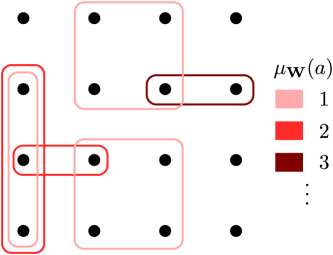
Figure 1: Sketch of a cluster ${\mathbf{W}}$ on a 2d square lattice (black dots). Each Pauli string $a$ contained in ${\mathbf{W}}$ is shown by a square loop, whose color represents its multiplicity $\mu_{\mathbf{W}}(a)$. As shown on the very left, two Pauli strings can be supported on an identical set of qubits. One can verify $|{\mathbf{W}}|=10$ and ${\mathbf{W}}!=24$ for this example. The cluster ${\mathbf{W}}$ is disconnected, and is the union ${\mathbf{W}}={\mathbf{V}}_{1}\cup{\mathbf{V}}_{2}$ of two connected clusters, where ${\mathbf{V}}_{1}$ (${\mathbf{V}}_{2}$) lies on the lower left (upper right).

Definition 6.

A cluster ${\mathbf{V}}$ is a multiset of $a$s, which assigns a multiplicity $\mu_{\mathbf{V}}(a)\in\{0,1,\cdots\}$ to each $a$. We also denote ${\mathbf{V}}=\{a,\cdots,a,b,\cdots\}$, where $a$ appears $\mu_{\mathbf{V}}(a)$ times. We say ${\mathbf{V}}$ contains $a$ (denoted by $a\in{\mathbf{V}}$) if $\mu_{\mathbf{V}}(a)\geq 1$. Define the total weight of ${\mathbf{V}}$ as $|{\mathbf{V}}|:=\sum_{a}\mu_{\mathbf{V}}(a)$, while ${\mathbf{V}}!:=\prod_{a}\left(\mu_{\mathbf{V}}(a)!\right)$ (note the difference to $|{\mathbf{V}}|!$) and $\lambda^{\mathbf{V}}:=\prod_{a}\lambda_{a}^{\mu_{{\mathbf{V}}}(a)}$.

Clusters can union with each other. For example, the cluster ${\mathbf{W}}={\mathbf{V}}_{1}\cup{\mathbf{V}}_{2}$ is defined by $\mu_{\mathbf{W}}(a)=\mu_{{\mathbf{V}}_{1}}(a)+\mu_{{\mathbf{V}}_{2}}(a),\forall a$.

A cluster ${\mathbf{W}}$ is called disconnected, if the $a$s contained in ${\mathbf{W}}$ can be separated to two sets $A_{1},A_{2}$, such that any pair $a_{1}\in A_{1},a_{2}\in A_{2}$ from the two sets do not overlap in their support qubits. Otherwise ${\mathbf{W}}$ is connected.

The proof idea is to first convert the fraction (16) to a logarithm that is easier to deal with. One can explicitly verify (generalizing Proposition 3.2 in Haah et al. (2021))

$$2p-1=\left.\partial_{\kappa}\log\mathcal{Z}\right|_{\kappa=0},$$ (22)

where

$$\mathcal{Z}:=2^{n-N}\mathrm{Tr}\left(E_{n}\mathrm{e}^{\kappa E_{j}}\mathrm{e}^{-\beta H}\right),$$ (23)

and $E_{j}$ is a Pauli operator on $j$ due to (21). We proceed to find the $\beta$-expansion for the “partition function” $\mathcal{Z}$ (c.f. (47) in Haah et al. (2021))

$$\mathcal{Z}= 2^{n-N}\left[\mathrm{Tr}\left(E_{n}\mathrm{e}^{\kappa E_{j}}\right)-\beta\mathrm{Tr}\left(E_{n}\mathrm{e}^{\kappa E_{j}}\textstyle{\sum_{a}}\lambda_{a}H_{a}\right)+\cdots\right]$$

$$= \cosh\kappa+\sum_{m=1}^{\infty}\sum_{{\mathbf{V}}:\left\lvert{\mathbf{V}}\right\rvert=m}\frac{\lambda^{\mathbf{V}}}{{\mathbf{V}}!}\mathcal{D}_{\mathbf{V}}\mathcal{Z}.$$ (24)

The sum is over all clusters ${\mathbf{V}}$, where

$$\mathcal{D}_{\mathbf{V}}\mathcal{Z}:=2^{n-N}\frac{(-\beta)^{m}}{m!}\sum_{\sigma\in\mathsf{S}_{m}}\mathrm{Tr}\left(E_{n}\mathrm{e}^{\kappa E_{j}}H_{a_{\sigma_{1}}}\cdots H_{a_{\sigma_{m}}}\right),$$ (25)

with ${\mathbf{V}}=\{a_{1},\cdots,a_{m}\}$, and $\mathsf{S}_{m}$ being the permutation group of $m$ elements. Intuitively, $\mathcal{D}_{\mathbf{V}}\mathcal{Z}$ is a derivative of $\mathcal{Z}$ over multi-variables $\{\lambda_{a}\}$ at $\lambda_{a}=0$. To get (A), we have expanded $H$ to local Paulis $H_{a}$ by (3), used $\mathrm{Tr}\left(E_{n}\right)=2^{N-n}$, and organized terms into clusters according to (25). The ${\mathbf{V}}!$ factor appears in (A) because, for example, there is only one $H_{a}H_{a}$ term in $H^{2}$, but that term is counted twice in (25).

Taking the logarithm of (A) and expanding in $\beta$, each final term may correspond to multiple clusters ${\mathbf{V}}_{1},{\mathbf{V}}_{2},\cdots$ in (A), which comes from higher orders in the expansion $\log(1+y)=y-y^{2}/2+\cdots$ with $y=\sum_{{\mathbf{V}}}\cdots$. These multiple clusters combine to a single one ${\mathbf{W}}={\mathbf{V}}_{1}\cup{\mathbf{V}}_{2}\cup\cdots$, and we organize the final terms according to the combined cluster: (see (25) in Haah et al. (2021))

$$\log\mathcal{Z}=\log\cosh\kappa+\sum_{m=1}^{\infty}\beta^{m}\sum_{{\mathbf{W}}:\left\lvert{\mathbf{W}}\right\rvert=m}\lambda^{\mathbf{W}}\varGamma_{{\mathbf{W}}}.$$ (26)

where $\varGamma_{{\mathbf{W}}}$ do not depend on $\beta$ and $\{\lambda_{a}\}$. Schematically,

$$\beta^{m}\varGamma_{\mathbf{W}}=\sum_{\{{\mathbf{V}}_{\ell}\}}\chi({\mathbf{W}},\{{\mathbf{V}}_{\ell}\})\prod_{\ell=1}^{L}\frac{\mathcal{D}_{{\mathbf{V}}_{\ell}}\mathcal{Z}}{\cosh\kappa},$$ (27)

where $\{{\mathbf{V}}_{\ell}\}$ denotes a multiset of connected clusters ${\mathbf{V}}_{1},{\mathbf{V}}_{2},\cdots,{\mathbf{V}}_{L}$ with $L\leq m$ that partitions the entire cluster ${\mathbf{W}}$, and the coefficient $\chi({\mathbf{W}},\{{\mathbf{V}}_{\ell}\})$ is determined by geometry alone. Using (22) to compare to (16), we identify

$$\gamma_{m}=\sum_{{\mathbf{W}}\ni j:\left\lvert{\mathbf{W}}\right\rvert=m}\lambda^{\mathbf{W}}\left(\partial_{\kappa}\varGamma_{\mathbf{W}}\right)_{0},$$ (28)

where $\left(\cdots\right)_{0}$ means taking $\kappa=0$. Here the sum is constrained to clusters ${\mathbf{W}}$ containing $j$, because if $j\notin{\mathbf{W}}$, $\mathcal{D}_{{\mathbf{V}}_{\ell}}\mathcal{Z}$ in (27) will depend on $\kappa$ simply by a multiplicative factor $\cosh\kappa$ according to (25):

$$\mathrm{Tr}\left(E_{n}\mathrm{e}^{\kappa E_{j}}O\right)\propto\mathrm{Tr}\left(E_{n}\mathrm{e}^{\kappa E_{j}}\right)\mathrm{Tr}\left(E_{n}O\right)\propto\cosh\kappa,$$ (29)

if $O=H_{a_{\sigma_{1}}}\cdots$ does not act on $j$. This factor cancels the $\kappa$-dependence in the denominator of (27), thus taking the $\kappa$-derivative simply yields zero.

Although general expressions for $\varGamma_{\mathbf{W}}$ are complicated, we know it always vanishes if ${\mathbf{W}}$ is disconnected: Suppose the $a$s contained in ${\mathbf{W}}$ belong to two disconnected sets of qubits $A_{1},A_{2}$, and we set $\lambda_{a}=0$ for all $a\notin{\mathbf{W}}$ , so that $H=H_{1}+H_{2}$ where $H_{1}$ ($H_{2}$) only acts inside $A_{1}$ ($A_{2}$). Then similar to (29), the trace factorizes

$$\mathrm{Tr}\left(E_{n}\mathrm{e}^{-\beta H}\right) =\mathrm{Tr}\left[\left(E_{n,1}\mathrm{e}^{\kappa E_{j}}\mathrm{e}^{-\beta H_{1}}\right)\otimes\left(E_{n,2}\mathrm{e}^{-\beta H_{2}}\right)\right]$$

$$\propto\mathrm{Tr}\left(E_{n}\mathrm{e}^{\kappa E_{j}}\mathrm{e}^{-\beta H_{1}}\right)\mathrm{Tr}\left(E_{n}\mathrm{e}^{-\beta H_{2}}\right),$$ (30)

where we have expressed the single-site projectors $E_{n}=E_{n,1}\otimes E_{n,2}$ with $E_{n,1}$ ($E_{n,2}$) acting inside (outside) $A_{1}$, and assumed $j\in A_{1}$ without loss of generality. As a result, $\log\mathcal{Z}=\zeta_{1}+\zeta_{2}$, where $\zeta_{1,2}$ is a multivariate polynomial of $\lambda_{a}$ for $a\in A_{1,2}$ alone. There are no cross terms like $\lambda_{a_{1}}\lambda_{a_{2}}$ where $a_{1}\in A_{1},a_{2}\in A_{2}$, which proves $\varGamma_{\mathbf{W}}=0$ because it is a coefficient of such cross terms.

Hence, the sum in (28) is further restricted to connected clusters of total weight $m$ that contains $j$. There are at most

$$C_{m}:=\mathrm{e}\mathfrak{d}\left[1+\mathrm{e}(\mathfrak{d}-1)\right]^{m-1}\leq(\mathrm{e}\mathfrak{d})^{m}$$ (31)

of them (Proposition 3.6 in Haah et al. (2021)), which can be enumerated in time $\mathrm{O}(m\mathfrak{d}C_{m})$ (Section 3.4 in Haah et al. (2021)).

Therefore, to prove (17), we only need to show that for each such cluster ${\mathbf{W}}$,

$$\left\lvert\left(\partial_{\kappa}\varGamma_{{\mathbf{W}}}\right)_{0}\right\rvert\leq m\left[2\mathrm{e}(\mathfrak{d}+1)\right]^{m}.$$ (32)

To proceed, we derive from (27)

$$\beta^{m}\left\lvert\left(\partial_{\kappa}\varGamma_{\mathbf{W}}\right)_{0}\right\rvert =\left\lvert\sum_{\{{\mathbf{V}}_{\ell}\}}\chi({\mathbf{W}},\{{\mathbf{V}}_{\ell}\})\sum_{\ell^{\prime}=1}^{L}\left(\partial_{\kappa}\mathcal{D}_{{\mathbf{V}}_{\ell^{\prime}}}\mathcal{Z}\right)_{0}\prod_{\ell=1,\ell\neq\ell^{\prime}}^{L}\left(\mathcal{D}_{{\mathbf{V}}_{\ell}}\mathcal{Z}\right)_{0}\right\rvert$$

$$\leq m\sum_{\{{\mathbf{V}}_{\ell}\}}\left\lvert\chi({\mathbf{W}},\{{\mathbf{V}}_{\ell}\})\right\rvert\beta^{\sum_{\ell}\left\lvert{\mathbf{V}}_{\ell}\right\rvert}=m\beta^{m}\sum_{\{{\mathbf{V}}_{\ell}\}}\left\lvert\chi({\mathbf{W}},\{{\mathbf{V}}_{\ell}\})\right\rvert.$$ (33)

Here we have used

$$\left\lvert\left(\partial_{\kappa}\mathcal{D}_{\mathbf{V}}\mathcal{Z}\right)_{0}\right\rvert,\left\lvert\left(\mathcal{D}_{\mathbf{V}}\mathcal{Z}\right)_{0}\right\rvert\leq\beta^{|{\mathbf{V}}|},$$ (34)

together with $L\leq m$ and the fact that $\{V_{\ell}\}$ partitions ${\mathbf{W}}$: $m=\sum_{\ell}\left\lvert{\mathbf{V}}_{\ell}\right\rvert$. We will prove (34) shortly; for now observe that what we need is a bound on the coefficient $\chi$. This is done precisely in Haah et al. (2021), where the major chunk of the proof establishes the right hand side of (32) as a bound for (A). Note that our $\chi$ is the same as what can be read out in eq.(50) of Haah et al. (2021), since it is merely a combinatorial factor that comes from expanding the logarithm, and does not depend on how $\mathcal{D}_{\mathbf{V}}\mathcal{Z}$ is defined in (25) (where there is no $E_{n}\mathrm{e}^{\kappa E_{j}}$ insertion in Haah et al. (2021)).

Now we show (34). Let $m=|{\mathbf{V}}|$. (25) leads to

$$\left\lvert\left(\mathcal{D}_{\mathbf{V}}\mathcal{Z}\right)_{0}\right\rvert \leq 2^{n-N}\beta^{m}\left\lVert E_{n}H_{a_{1}}\cdots H_{a_{m}}\right\rVert_{1}$$

$$\leq 2^{n-N}\beta^{m}\left\lVert E_{n}\right\rVert_{1}\left\lVert H_{a_{1}}\cdots H_{a_{m}}\right\rVert_{\infty}=\beta^{m}.$$ (35)

Here in the first line, we have used that the number of permutations is $|\mathsf{S}_{m}|=m!$ and $\mathrm{Tr}\left(A\right)\leq\left\lVert A\right\rVert_{1}:=\mathrm{Tr}\left(\sqrt{A^{\dagger}A}\right)$. In the second line, we have used Hölder inequality $\left\lVert AB\right\rVert_{1}\leq\left\lVert A\right\rVert_{1}\left\lVert B\right\rVert_{\infty}$, together with $\left\lVert H_{a_{1}}\cdots H_{a_{m}}\right\rVert_{\infty}\leq\left\lVert H_{a_{1}}\right\rVert_{\infty}\cdots\left\lVert H_{a_{m}}\right\rVert_{\infty}=1$ and $\left\lVert E_{n}\right\rVert_{1}=\mathrm{Tr}\left(E_{n}\right)=2^{N-n}$. As one can verify, $\left(\partial_{\kappa}\mathcal{D}_{\mathbf{V}}\mathcal{Z}\right)_{0}$ is bounded similarly by inserting $E_{j}$ in (A). As a result, (34) then establishes (32) following Haah et al. (2021), from which (17) is obtained.

Finally, to prove Lemma 5, we need to show that $\left(\partial_{\kappa}\varGamma_{\mathbf{W}}\right)_{0}$ can be computed in time

$$t_{\mathrm{compute}}=\mathrm{O}\left[2^{m(2k-1)}\mathrm{poly}\left(m\right)\right].$$ (36)

Haah et al. (2021) (Section 3.6) shows that $\varGamma_{\mathbf{W}}$ is computable in time

$$\mathrm{O}(8^{m}\mathrm{poly}\left(m\right)),$$ (37)

without the $E_{n}\mathrm{e}^{\kappa E_{j}}$ insertion, via taking multivariate derivative $\mathcal{D}_{\mathbf{W}}$ on $\log\mathcal{Z}$ (see (26)). Here we show that the insertion does not change this scaling much. The only subroutine in Haah et al. (2021) where $E_{n}\mathrm{e}^{\kappa E_{j}}$ would appear is to calculate

$$\mathrm{Tr}\left(E_{n}\mathrm{e}^{\kappa E_{j}}\mathcal{M}^{\mathcal{K}}\right)=\mathrm{Tr}\left(E_{n}\mathcal{M}^{\mathcal{K}}\right)+\kappa\mathrm{Tr}\left(E_{n}E_{j}\mathcal{M}^{\mathcal{K}}\right)+\cdots,$$ (38)

for $\mathcal{K}=1,\cdots,m$, where the matrix $\mathcal{M}:=\sum_{a\in{\mathbf{W}}}z_{a}H_{a}$ with $z_{a}$ being integers. We have expanded (38) in $\kappa$, so that what is really computed is the $c$-number coefficients. This is more complicated than Haah et al. (2021) where (38) is a single $c$-number $\mathrm{Tr}\left(\mathcal{M}^{\mathcal{K}}\right)$. However, this only yields an extra constant factor for the total complexity, because only the first derivative in $\kappa$ is needed in the end, so in each step of the calculation one can throw away $\kappa^{2}$ and higher orders. In other words, we only need to show that computing the first two orders in (38) requires a similar runtime as $\mathrm{Tr}\left(\mathcal{M}^{\mathcal{K}}\right)$, which is $\mathrm{O}(4^{m}\mathrm{poly}\left(m\right))$ shown in Haah et al. (2021).

We focus on the first term in (38), since the second follows similarly. Observe that computing that term can be restricted to no more than $1+m(k-1)$ qubits that support ${\mathbf{W}}$, since $E_{n}$ is a tensor product. This number of qubits is because the connected cluster ${\mathbf{W}}$ can be generated by starting from one $k$-local term $a\in{\mathbf{W}}$, and then gradually appending terms in ${\mathbf{W}}$ to it while keeping connectivity; each time appending one term adds at most $k-1$ support qubits. In other words, the first term in (38) is restricted to a Hilbert space of dimension $D=\mathrm{O}[2^{m(k-1)}]$. Furthermore, the matrix $\mathcal{M}=\sum_{a}z_{a}H_{a}$ to be powered is sparse: each row/column contains at most $m$ nonzero entries, so multiplying any matrix to it yields complexity $\mathrm{O}(D^{2})=\mathrm{O}[4^{m(k-1)}]$. This is the dominant complexity of (38) up to $\mathrm{poly}\left(m\right)$, so comparing to $\mathrm{O}(4^{m})$ without $E_{n}\mathrm{e}^{\kappa E_{j}}$ insertion, the computation time for $\left(\partial_{\kappa}\varGamma_{\mathbf{W}}\right)_{0}$ is given by (36) comparing to (37) following Haah et al. (2021).

Appendix B Proof of Theorem 3

We sketch the proof since it is very similar to Appendix A. Define $\mathcal{Z}^{\prime}$ in a similar way as (23) with replacement

$$\kappa E_{j}\rightarrow\kappa_{i}E_{i}+\kappa_{j}E_{j},$$ (39)

where $E_{i},E_{j}$ are the ones achieving the maximum in (3), and define $\varGamma^{\prime}_{\mathbf{W}}$ as the coefficient of the corresponding expansion in (26). Observe that

$$\mathrm{Cor}(i,j)=\left(\partial_{\kappa_{i}}\partial_{\kappa_{j}}\log\mathcal{Z}^{\prime}\right)_{0}$$

$$=\sum_{m=1}^{\infty}\beta^{m}\sum_{\begin{subarray}{c}{\mathbf{W}}\text{ connected}:\\ \{i,j\}\subset{\mathbf{W}},\left\lvert{\mathbf{W}}\right\rvert=m\end{subarray}}\lambda^{\mathbf{W}}\left(\partial_{\kappa_{i}}\partial_{\kappa_{j}}\varGamma_{{\mathbf{W}}}^{\prime}\right)_{0},$$ (40)

Here the first line comes from explicit calculation similar to (22), while the second line follows from generalizing the arguments around (29) and (A). For a connected cluster ${\mathbf{W}}$ that contains $i$ and $j$, the total weight cannot be too small: $m=\mathrm{\Omega}(\mathsf{d}(i,j))$. As a result, (3) then follows from (31) and a generalization of (32):

$$\left\lvert\left(\partial_{\kappa_{i}}\partial_{\kappa_{j}}\varGamma^{\prime}_{{\mathbf{W}}}\right)_{0}\right\rvert\leq m^{2}\left[2\mathrm{e}(\mathfrak{d}+1)\right]^{m}.$$ (41)

This holds by generalizing (A) to two derivatives, and (34) to

$$\left\lvert\left(\partial_{\kappa_{i}}\partial_{\kappa_{j}}\mathcal{D}_{\mathbf{V}}\mathcal{Z}^{\prime}\right)_{0}\right\rvert,\left\lvert\left(\partial_{\kappa_{i}}\mathcal{D}_{\mathbf{V}}\mathcal{Z}^{\prime}\right)_{0}\right\rvert,\left\lvert\left(\mathcal{D}_{\mathbf{V}}\mathcal{Z}^{\prime}\right)_{0}\right\rvert\leq\beta^{|{\mathbf{V}}|},$$ (42)

which comes from, e.g. $\left(\mathcal{D}_{\mathbf{V}}\mathcal{Z}^{\prime}\right)_{0}=\left(\mathcal{D}_{\mathbf{V}}\mathcal{Z}\right)_{0}$ and (A).

References

- Barahona (1982) F Barahona, “On the computational complexity of ising spin glass models,” Journal of Physics A: Mathematical and General 15, 3241 (1982).
- Lucas (2014) Andrew Lucas, “Ising formulations of many NP problems,” Frontiers in Physics 2, 5 (2014).
- Jerrum et al. (1986) Mark R. Jerrum, Leslie G. Valiant, and Vijay V. Vazirani, “Random generation of combinatorial structures from a uniform distribution,” Theoretical Computer Science 43, 169–188 (1986).
- Jerrum and Sinclair (1993) Mark Jerrum and Alistair Sinclair, “Polynomial-time approximation algorithms for the ising model,” SIAM Journal on Computing 22, 1087–1116 (1993).
- Randall and Wilson (1999) Dana Randall and David Wilson, “Sampling spin configurations of an ising system,” in Proceedings of the Tenth Annual ACM-SIAM Symposium on Discrete Algorithms, SODA ’99 (Society for Industrial and Applied Mathematics, USA, 1999) p. 959–960.
- Levin et al. (2009) D. A. Levin, Y. Peres, and E. L. Wilmer, Markov Chains and Mixing Times (AMS, 2009).
- Troyer and Wiese (2005) Matthias Troyer and Uwe-Jens Wiese, “Computational complexity and fundamental limitations to fermionic quantum monte carlo simulations,” Phys. Rev. Lett. 94, 170201 (2005).
- Dornheim (2019) T. Dornheim, “Fermion sign problem in path integral monte carlo simulations: Quantum dots, ultracold atoms, and warm dense matter,” Phys. Rev. E 100, 023307 (2019).
- Diedrich and Anderson (1992) D. L. Diedrich and J. B. Anderson, “An accurate quantum Monte Carlo calculation of the barrier height for the reaction ,” Science 258, 786 (1992).
- Creutz et al. (1983) M. Creutz, L. Jacobs, and C. Rebbi, “Monte Carlo computations in lattice gauge theories,” Phys. Rep. 95, 201 (1983).
- Carlson et al. (2015) J. Carlson, S. Gandolfi, F. Pederiva, Steven C. Pieper, R. Schiavilla, K. E. Schmidt, and R. B. Wiringa, “Quantum monte carlo methods for nuclear physics,” Rev. Mod. Phys. 87, 1067–1118 (2015).
- White et al. (1989) S. R. White, D. J. Scalapino, R. L. Sugar, E. Y. Loh, J. E. Gubernatis, and R. T. Scalettar, “Numerical study of the two-dimensional hubbard model,” Phys. Rev. B 40, 506–516 (1989).
- Bravyi et al. (2008) Sergey Bravyi, David P. DiVincenzo, Roberto I. Oliveira, and Barbara M. Terhal, “The complexity of stoquastic local hamiltonian problems,” Quant. Inf. Comp. 8, 361 (2008), arXiv:quant-ph/0606140 [quant-ph] .
- Barrett et al. (2009) Sean D. Barrett, Stephen D. Bartlett, Andrew C. Doherty, David Jennings, and Terry Rudolph, “Transitions in the computational power of thermal states for measurement-based quantum computation,” Phys. Rev. A 80, 062328 (2009).
- Bravyi and Gosset (2017) Sergey Bravyi and David Gosset, “Polynomial-time classical simulation of quantum ferromagnets,” Phys. Rev. Lett. 119, 100503 (2017).
- Li and Yao (2019) Zi-Xiang Li and Hong Yao, “Sign-problem-free fermionic quantum monte carlo: Developments and applications,” Ann. Rev. Cond. Mat. Phys. 10, 337–356 (2019).
- Crosson and Slezak (2020) Elizabeth Crosson and Samuel Slezak, “Classical simulation of high temperature quantum ising models,” (2020), arXiv:2002.02232 .
- Crosson and Harrow (2021) Elizabeth Crosson and Aram W. Harrow, “Rapid mixing of path integral Monte Carlo for 1D stoquastic Hamiltonians,” Quantum 5, 395 (2021).
- Kliesch et al. (2014) M. Kliesch, C. Gogolin, M. J. Kastoryano, A. Riera, and J. Eisert, “Locality of temperature,” Phys. Rev. X 4, 031019 (2014).
- Kuwahara et al. (2020) Tomotaka Kuwahara, Kohtaro Kato, and Fernando G. S. L. Brandão, “Clustering of conditional mutual information for quantum gibbs states above a threshold temperature,” Phys. Rev. Lett. 124, 220601 (2020).
- Brandão and Kastoryano (2019) Fernando G. S. L. Brandão and Michael J. Kastoryano, “Finite Correlation Length Implies Efficient Preparation of Quantum Thermal States,” Commun. Math. Phys. 365, 1–16 (2019), arXiv:1609.07877 [quant-ph] .
- Terhal and DiVincenzo (2004) Barbara M. Terhal and David P. DiVincenzo, “Adaptive quantum computation, constant depth quantum circuits and arthur-merlin games,” Quantum Info. Comput. 4, 134–145 (2004).
- Harrow et al. (2020) Aram W. Harrow, Saeed Mehraban, and Mehdi Soleimanifar, “Classical algorithms, correlation decay, and complex zeros of partition functions of quantum many-body systems,” in Proceedings of the 52nd Annual ACM SIGACT Symposium on Theory of Computing, STOC 2020 (Association for Computing Machinery, New York, NY, USA, 2020) p. 378–386.
- Bravyi et al. (2022) Sergey Bravyi, Anirban Chowdhury, David Gosset, and Pawel Wocjan, “Quantum hamiltonian complexity in thermal equilibrium,” Nature Physics 18, 1367–1370 (2022).
- Alhambra and Cirac (2021) Álvaro M. Alhambra and J. Ignacio Cirac, “Locally accurate tensor networks for thermal states and time evolution,” PRX Quantum 2, 040331 (2021).
- Bluhm et al. (2022) Andreas Bluhm, Ángela Capel, and Antonio Pérez-Hernández, “Exponential decay of mutual information for Gibbs states of local Hamiltonians,” Quantum 6, 650 (2022).
- Chi-Fang et al. (2023) Chi-Fang, Chen, Michael J. Kastoryano, Fernando G. S. L. Brandão, and András Gilyén, “Quantum Thermal State Preparation,” (2023), arXiv:2303.18224 [quant-ph] .
- Alhambra (2022) Álvaro M. Alhambra, “Quantum many-body systems in thermal equilibrium,” (2022) arXiv:2204.08349 [quant-ph] .
- Li et al. (2011) Ying Li, Daniel E. Browne, Leong Chuan Kwek, Robert Raussendorf, and Tzu-Chieh Wei, “Thermal states as universal resources for quantum computation with always-on interactions,” Phys. Rev. Lett. 107, 060501 (2011).
- Fujii et al. (2013) Keisuke Fujii, Yoshifumi Nakata, Masayuki Ohzeki, and Mio Murao, “Measurement-based quantum computation on symmetry breaking thermal states,” Phys. Rev. Lett. 110, 120502 (2013).
- Bremner et al. (2017) Michael J. Bremner, Ashley Montanaro, and Dan J. Shepherd, “Achieving quantum supremacy with sparse and noisy commuting quantum computations,” Quantum 1, 8 (2017).
- Haah et al. (2021) Jeongwan Haah, Robin Kothari, and Ewin Tang, “Optimal learning of quantum Hamiltonians from high-temperature Gibbs states,” (2021) arXiv:2108.04842 [quant-ph] .
- Wild and Alhambra (2022) Dominik S. Wild and Álvaro M. Alhambra, “Classical simulation of short-time quantum dynamics,” (2022), arXiv:2210.11490 [quant-ph] .
- Bravyi and Kitaev (2002) Sergey B. Bravyi and Alexei Yu. Kitaev, “Fermionic quantum computation,” Annals of Physics 298, 210–226 (2002).
- Verstraete and Cirac (2005) F. Verstraete and J. I. Cirac, “Mapping local Hamiltonians of fermions to local Hamiltonians of spins,” J. Stat. Mech. 0509, P09012 (2005), arXiv:cond-mat/0508353 .
- Setia et al. (2019) Kanav Setia, Sergey Bravyi, Antonio Mezzacapo, and James D. Whitfield, “Superfast encodings for fermionic quantum simulation,” Phys. Rev. Res. 1, 033033 (2019).
- Derby et al. (2021) Charles Derby, Joel Klassen, Johannes Bausch, and Toby Cubitt, “Compact fermion to qubit mappings,” Phys. Rev. B 104, 035118 (2021).
- Yin and Lucas (2023) C. Yin and A. Lucas, “to appear,” (2023).
- Raussendorf and Briegel (2001) Robert Raussendorf and Hans J. Briegel, “A one-way quantum computer,” Phys. Rev. Lett. 86, 5188–5191 (2001).