A Rainbow in Deep Network Black Boxes

Abstract

We introduce rainbow networks as a probabilistic model of trained deep neural networks. The model cascades random feature maps whose weight distributions are learned. It assumes that dependencies between weights at different layers are reduced to rotations which align the input activations. Neuron weights within a layer are independent after this alignment. Their activations define kernels which become deterministic in the infinite-width limit. This is verified numerically for ResNets trained on the ImageNet dataset. We also show that the learned weight distributions have low-rank covariances. Rainbow networks thus alternate between linear dimension reductions and non-linear high-dimensional embeddings with white random features. Gaussian rainbow networks are defined with Gaussian weight distributions. These models are validated numerically on image classification on the CIFAR-10 dataset, with wavelet scattering networks. We further show that during training, SGD updates the weight covariances while mostly preserving the Gaussian initialization.

Keywords: deep neural networks, infinite-width limit, weight probability distribution, random features, network alignment.

1 Introduction

Deep neural networks have been described as black boxes because many of their fundamental properties are not understood. Their weight matrices are learned by performing stochastic gradient descent from a random initialization. Each training run thus results in a different set of weight matrices, which can be considered as a random realization of some probability distribution. What is this probability distribution? What is the corresponding functional space? Do all networks learn the same function, and even the same weights, up to some symmetries? This paper addresses these questions.

Theoretical studies have mostly focused on shallow learning. A first line of work has studied learning of the last layer while freezing the other ones. The previous layers thus implement random features (Jarrett et al., 2009; Pinto et al., 2009) which specify a kernel that becomes deterministic in the infinite-width limit (Rahimi and Recht, 2007; Daniely et al., 2016). Learning has then been incorporated in these models. Neal (1996); Williams (1996); Lee et al. (2018); Matthews et al. (2018) show that some networks behave as Gaussian processes. Training is then modeled as sampling from the Bayesian posterior given the training data. On the other hand, Jacot et al. (2018) and Lee et al. (2019) assume that trained weights have small deviations from their initialization. In these cases, learning is in a “lazy” regime (Chizat et al., 2019) specified by a fixed kernel. It has been opposed to a “rich” or feature-learning regime (Chizat and Bach, 2020; Woodworth et al., 2020), which achieves higher performance on complex tasks (Lee et al., 2020; Geiger et al., 2020). Empirical observations of weight statistics have indeed shown that they significantly evolve during training (Martin and Mahoney, 2021; Thamm et al., 2022). This has been precisely analyzed for one-hidden-layer networks in the infinite-width “mean-field” limit (Chizat and Bach, 2018; Mei et al., 2018; Rotskoff and Vanden-Eijnden, 2018; Sirignano and Spiliopoulos, 2020), which allows tracking the neuron weight distribution as it evolves away from the Gaussian initialization during training. The generalization to deeper networks is greatly complicated by the fact that intermediate activations depend on the random weight realizations (Sirignano and Spiliopoulos, 2022; E and Wojtowytsch, 2020; Nguyen and Pham, 2020; Chen et al., 2022; Yang and Hu, 2021). However, numerical experiments (Raghu et al., 2017; Kornblith et al., 2019) show that intermediate activations correlate significantly across independent realizations, which calls for an explanation of this phenomenon.

Building upon these ideas, we introduce the rainbow model of the joint probability distribution of trained network weights across layers. It assumes that dependencies between the weight matrices $W_{j}$ at all layers $j$ are reduced to rotations. This means that $W_{j}=W^{\prime}_{j}\hat{A}_{j-1}$, where $W^{\prime}_{1},\dots,W^{\prime}_{J}$ are independent random matrices, and $\hat{A}_{j-1}$ is a rotation that depends on the previous layer weights $W_{1},\dots,W_{j-1}$. The $W^{\prime}_{j}$ are further assumed to be random feature matrices, that is, their rows are independent and identically distributed.

The functional properties of rainbow networks depend on the random feature distribution at each layer. We show numerically that weights of trained networks typically have low-rank covariances. The corresponding rainbow networks thus implement dimensionality reductions in-between the high-dimensional random feature embeddings, similar to previous works (Cho and Saul, 2009; Mairal, 2016; Bietti, 2019). We further demonstrate that input activation covariances provide efficient approximations of the eigenspaces of the weight covariances. The number of model parameters and hence the supervised learning complexity can thus be considerably reduced by unsupervised information.

The weight covariances completely specify the rainbow network output and properties when the weight distributions are Gaussian. The eigenvectors of these weight covariances can be interpreted as learned features, rather than individual neuron weights which are random. This Gaussian assumption is too restrictive to model arbitrary trained networks. However, it can approximately hold for architectures which incorporate prior information and restrict their learned weights. In some of our numerical experiments, we will thus consider learned scattering networks (Zarka et al., 2021; Guth et al., 2022), which have fixed wavelet spatial filters and learn weights along channels only.

This paper makes the following main contributions:

• We prove that the rainbow network activations converge to a random rotation of a deterministic kernel feature vector in the infinite-width limit, which explains the empirical results of representation similarity of Raghu et al. (2017) and Kornblith et al. (2019). We verify numerically this convergence on scattering networks and ResNets trained on the CIFAR-10 and ImageNet image classification datasets. We conjecture but do not prove that this convergence conversely implies the first rainbow assumption that layer dependencies are reduced to rotations.

• We validate the Gaussian rainbow model for scattering networks trained on CIFAR-10. We verify that the weight covariances converge up to rotation when the width increases, and that the weights are approximately Gaussian. The weight covariances are sufficient to sample rainbow weights and define new networks that achieve comparable classification accuracy as the original trained network when the width is large enough. Further, we show that SGD training only updates the weight covariances while nearly preserving the white random feature initializations, suggesting a possible explanation for the Gaussian rainbow assumption in this setting.

• We prove that equivariance to general groups can be achieved in rainbow networks with weight distributions that are invariant to the group action. This constraint on distributions rather than on individual neurons (Cohen and Welling, 2016; Kondor and Trivedi, 2018) avoids any weight sharing or synchronizations, which are difficult to implement in biological systems.

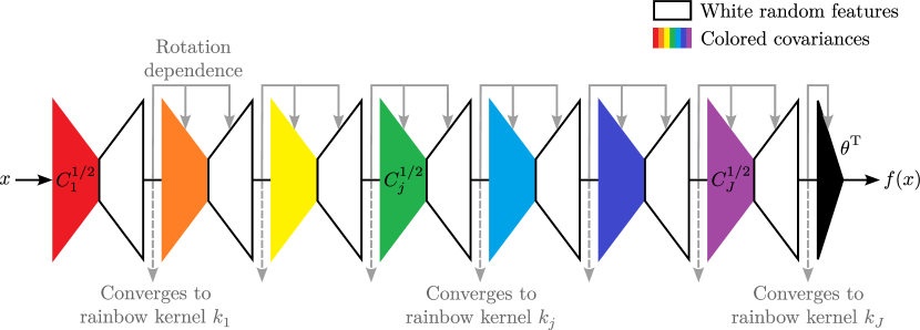
Figure 1: A deep rainbow network cascades random feature maps whose weight distributions are learned. They typically have a low-rank covariance. Each layer can be factorized into a linear dimensionality reduction determined by the colored covariance, followed by a non-linear high-dimensional embedding with white random features. At each layer, the hidden activations define a kernel which converges to a deterministic rainbow kernel in the infinite width limit. It induces a random rotation of the next layer weights. For Gaussian rainbow networks, the random feature embedding is a dot-product kernel feature map which does not need to be rotated.

The rainbow model is illustrated in Figure 1. In Section 2, we introduce rainbow networks and the associated kernels that describe their infinite-width limit. We validate numerically the above properties and results in Section 3.

2 Rainbow networks

Weight matrices of learned deep networks are strongly dependent across layers. Deep rainbow networks define a mathematical model of these dependencies through rotation matrices that align input activations at each layer. We review in Section 2.1 the properties of random features, which are the building blocks of the model. We then introduce in Section 2.2 deep fully-connected rainbow networks, which cascade aligned random feature maps. We show in Section 2.3 how to incorporate inductive biases in the form of symmetries or local neuron receptive fields. We also extend rainbow models to convolutional networks.

2.1 Rotations in random feature maps

We being by reviewing the properties of one-hidden layer random feature networks. We then prove that random weight fluctuations produce a random rotation of the hidden activation layer in the limit of infinite layer width. The rainbow network model will be obtained by applying this result at all layers of a deep network.

Random feature network.

A one-hidden layer network computes a hidden activation layer with a matrix $W$ of size $d_{1}\times d_{0}$ and a pointwise non-linearity $\rho$:

$$\hat{\varphi}(x)=\rho(Wx)\leavevmode\nobreak\ \leavevmode\nobreak\ \mbox{for}\leavevmode\nobreak\ \leavevmode\nobreak\ x\in{\mathbb{R}}^{d_{0}}.$$

We consider a random feature network (Rahimi and Recht, 2007). The rows of $W$, which contain the weights of different neurons, are independent and have the same probability distribution $\pi$:

$$W=(w_{i})_{i\leq d_{1}}\leavevmode\nobreak\ \leavevmode\nobreak\ \mbox{with i.i.d.}\leavevmode\nobreak\ \leavevmode\nobreak\ w_{i}\sim\pi.$$

In many random feature models, each row vector has a known distribution with uncorrelated coefficients (Jarrett et al., 2009; Pinto et al., 2009). Learning is then reduced to calculating the output weights $\hat{\theta}$, which define

$$\hat{f}(x)={\langle}\hat{\theta},\hat{\varphi}(x){\rangle}.$$

In contrast, we consider general distributions $\pi$ which will be estimated from the weights of trained networks in Section 3.

Our network does not include any bias for simplicity. Bias-free networks have been shown to achieve comparable performance as networks with biases for denoising (Mohan et al., 2019) and image classification (Zarka et al., 2021; Guth et al., 2022). However, biases can easily be incorporated in random feature models and thus rainbow networks.

We consider a normalized network, where $\rho$ includes a division by $\sqrt{d_{1}}$ so that ${\mathopen{}\mathclose{{}\left\lVert\hat{\varphi}(x)}\right\rVert}$ remains of the order of unity when the width $d_{1}$ increases. We shall leave this normalization implicit to simplify notations, except when illustrating mathematical convergence results. Note that this choice differs from the so-called standard parameterization (Yang and Hu, 2021). In numerical experiments, we perform SGD training with this standard parameterization which avoids getting trapped in the lazy training regime (Chizat et al., 2019). Our normalization convention is only applied at the end of training, where the additional factor of $\sqrt{d_{1}}$ is absorbed in the next-layer weights $\hat{\theta}$.

We require that the input data has finite energy: $\mathbb{E}_{x}[{\mathopen{}\mathclose{{}\left\lVert x}\right\rVert}^{2}]<+\infty$. We further assume that the non-linearity $\rho$ is Lipschitz, which is verified by many non-linearities used in practice, including ReLU. Finally, we require that the random feature distribution $\pi$ has finite fourth-order moments.

Kernel convergence.

We now review the convergence properties of one-hidden layer random feature networks. This convergence is captured by the convergence of their kernel (Rahimi and Recht, 2007, 2008),

$$\hat{k}(x,x^{\prime})=\langle\hat{\varphi}(x),\hat{\varphi}(x^{\prime})\rangle=\frac{1}{d_{1}}\sum_{i=1}^{d_{1}}\rho\mathopen{}\mathclose{{}\left(\mathopen{}\mathclose{{}\left\langle x,w_{i}}\right\rangle}\right)\,\rho(\langle x^{\prime},w_{i}\rangle),$$

where we have made explicit the factor $d_{1}^{-1}$ coming from our choice of normalization. Since the rows $w_{i}$ are independent and identically distributed, the law of large numbers implies that when the width $d_{1}$ goes to infinity, this empirical kernel has a mean-square convergence to the asymptotic kernel

$$k(x,x^{\prime})=\mathbb{E}_{w\sim\pi}\mathopen{}\mathclose{{}\left[\rho\mathopen{}\mathclose{{}\left(\mathopen{}\mathclose{{}\left\langle x,w}\right\rangle}\right)\,\rho(\langle x^{\prime},w\rangle)}\right].$$ (1)

This convergence means that even though $\hat{\varphi}$ is random, its geometry (as described by the resulting kernel) is asymptotically deterministic. As we will see, this imposes that random fluctuations of $\hat{\varphi}(x)$ are reduced to rotations.

Let $\varphi(x)$ be an infinite-dimensional deterministic colored feature vector in a separable Hilbert space $H$, which satisfies

$$\langle\varphi(x),\varphi(x^{\prime})\rangle_{H}=k(x,x^{\prime}).$$ (2)

Such feature vectors always exist (Aronszajn, 1950, see also Schölkopf and Smola, 2002). For instance, one can choose $\varphi(x)=\mathopen{}\mathclose{{}\left(\rho(\mathopen{}\mathclose{{}\left\langle x,w}\right\rangle)}\right)_{w}$, the infinite-width limit of random features $\rho W$. In that case, $H=L^{2}(\pi)$, that is, the space of square-integrable functions with respect to $\pi$, with dot-product $\mathopen{}\mathclose{{}\left\langle g,h}\right\rangle_{H}=\mathbb{E}_{w\sim\pi}[g(w)\,h(w)]$. This choice is however not unique: one can obtain other feature vectors defined in other Hilbert spaces by applying a unitary transformation to $\varphi$, which does not modify the dot product in eq. 2. In the following, we choose the kernel PCA (KPCA) feature vector, whose covariance matrix $\mathbb{E}_{x}[\varphi(x)\,\varphi(x)^{\mathrm{T}}]$ is diagonal with decreasing values along the diagonal, introduced by Schölkopf et al. (1997). It is obtained by expressing any feature vector $\varphi$ in its PCA basis relative to the distribution of $x$. In this case $H=\ell^{2}({\mathbb{N}})$.

Finally, we denote by $\cal H$ the reproducing kernel Hilbert space (RKHS) associated to the kernel $k$ in eq. 1. It is the space of functions $f$ which can be written $f(x)=\mathopen{}\mathclose{{}\left\langle\theta,\varphi(x)}\right\rangle_{H}$, with norm ${\mathopen{}\mathclose{{}\left\lVert f}\right\rVert}_{\mathcal{H}}={\mathopen{}\mathclose{{}\left\lVert\theta}\right\rVert}_{H}$. A random feature network defines approximations of functions in this RKHS. With $H=L^{2}(\pi)$, these functions can be written

$$f(x)=\mathbb{E}_{w\sim\pi}\mathopen{}\mathclose{{}\left[\theta(w)\,\rho(\mathopen{}\mathclose{{}\left\langle x,w}\right\rangle)}\right]=\int\theta(w)\,\rho(\mathopen{}\mathclose{{}\left\langle x,w}\right\rangle)\,\mathrm{d}\pi(w).$$

This expression is equivalent to the mean-field limit of one-hidden-layer networks (Chizat and Bach, 2018; Mei et al., 2018; Rotskoff and Vanden-Eijnden, 2018; Sirignano and Spiliopoulos, 2020), which we will generalize to deep networks in Section 2.2.

Rotation alignment.

We now introduce rotations which align approximate kernel feature vectors. By abuse of language, we use rotations as a synonym for orthogonal transformations, and also include improper rotations which are the composition of a rotation with a reflection.

We have seen that the kernel $\hat{k}(x,x^{\prime})={\langle}\hat{\varphi}(x),\hat{\varphi}(x^{\prime}){\rangle}$ converges to the kernel $k(x,x^{\prime})={\langle}\varphi(x),\varphi(x^{\prime}){\rangle}$. We thus expect (and will later prove) that there exists a rotation $\hat{A}$ such that $\hat{A}\,\hat{\varphi}\approx\varphi$ because all feature vectors of the kernel $k$ are rotations of one another. The rotation $\hat{A}$ is dependent on the random feature realization $W$ and is thus random. The network activations $\hat{\varphi}(x)\approx\hat{A}^{\mathrm{T}}\varphi(x)$ are therefore a random rotation of the deterministic feature vector $\varphi(x)$. For the KPCA feature vector $\varphi$, $\hat{A}$ approximately computes an orthonormal change of coordinate of $\hat{\varphi}(x)$ to its PCA basis.

For any function $f(x)=\mathopen{}\mathclose{{}\left\langle\theta,\varphi(x)}\right\rangle_{H}$ in $\mathcal{H}$, if the output layer weights are $\hat{\theta}=\hat{A}^{\mathrm{T}}\theta$, then the network output is

$$\hat{f}(x)=\langle\hat{A}^{\mathrm{T}}\theta,\hat{\varphi}(x)\rangle=\langle\theta,\hat{A}\,\hat{\varphi}(x)\rangle_{H}\approx f(x).$$

This means that the final layer coefficients $\hat{\theta}$ can cancel the random rotation $\hat{A}$ introduced by $W$, so that the random network output $\hat{f}(x)$ converges when the width $d_{1}$ increases to a fixed function in $\cal H$. This propagation of rotations across layers is key to understanding the weight dependencies in deep networks. We now make the above arguments more rigorous and prove that $\hat{\varphi}$ and $\hat{f}$ respectively converge to $\varphi$ and $f$, for an appropriate choice of $\hat{A}$.

We write ${\cal O}(d_{1})$ the set of linear operators $A$ from ${\mathbb{R}}^{d_{1}}$ to $H=\ell^{2}(\mathbb{N})$ which satisfy $A^{\mathrm{T}}A=\mathrm{Id}_{d_{1}}$. Each $A\in\mathcal{O}(d_{1})$ computes an isometric embedding of $\mathbb{R}^{d_{1}}$ into $H$, while $A^{\mathrm{T}}$ is an orthogonal projection onto a $d_{1}$-dimensional subspace of $H$ which can be identified with $\mathbb{R}^{d_{1}}$. The alignment $\hat{A}$ of $\hat{\varphi}$ to $\varphi$ is defined as the minimizer of the mean squared error:

$$\hat{A}=\operatorname*{arg\,min}_{\hat{A}\in{\cal O}(d_{1})}\ \mathbb{E}_{x}\mathopen{}\mathclose{{}\left[{\lVert\hat{A}\,\hat{\varphi}(x)-\varphi(x)\rVert}^{2}_{H}}\right].$$ (3)

This optimization problem, known as the (orthogonal) Procrustes problem (Hurley and Cattell, 1962; Schönemann, 1966), admits a closed-form solution, computed from a singular value decomposition of the (uncentered) cross-covariance matrix between $\varphi$ and $\hat{\varphi}$:

$$\hat{A}=UV^{\mathrm{T}}\leavevmode\nobreak\ \leavevmode\nobreak\ \text{with}\leavevmode\nobreak\ \leavevmode\nobreak\ \mathbb{E}_{x}\mathopen{}\mathclose{{}\left[\varphi(x)\,\hat{\varphi}(x)^{\mathrm{T}}}\right]=USV^{\mathrm{T}}.$$ (4)

The mean squared error (3) of the optimal $\hat{A}$ (4) is then

$$\mathbb{E}_{x}\mathopen{}\mathclose{{}\left[{\lVert\hat{A}\,\hat{\varphi}(x)-\varphi(x)\rVert}^{2}_{H}}\right]=\operatorname{tr}{\mathbb{E}_{x}\mathopen{}\mathclose{{}\left[\hat{\varphi}(x)\,\hat{\varphi}(x)^{\mathrm{T}}}\right]}+\operatorname{tr}{\mathbb{E}_{x}\mathopen{}\mathclose{{}\left[\varphi(x)\,\varphi(x)^{\mathrm{T}}}\right]}-2{\mathopen{}\mathclose{{}\left\lVert\mathbb{E}_{x}\mathopen{}\mathclose{{}\left[\varphi(x)\,\hat{\varphi}(x)^{\mathrm{T}}}\right]}\right\rVert}_{1},$$ (5)

where ${\mathopen{}\mathclose{{}\left\lVert\cdot}\right\rVert}_{1}$ is the nuclear (or trace) norm, that is, the sum of the singular values. Equation 5 defines a distance between the representations $\hat{\varphi}$ and $\varphi$ which is related to various similarity measures used in the literature.

The alignment rotation (3,4) was used by Haxby et al. (2011) to align fMRI response patterns of human visual cortex from different individuals, and by Smith et al. (2017) to align word embeddings from different languages. Alignment between network weights has also been considered in previous works, but it was restricted to permutation matrices (Entezari et al., 2022; Benzing et al., 2022; Ainsworth et al., 2022). Permutations have the advantage of commuting with pointwise non-linearities, and can therefore be introduced while exactly preserving the network output function. However, they are not sufficiently rich to capture the variability of random features. It is shown in Entezari et al. (2022) that the error after permutation alignment converges to zero with the number of random features $d_{1}$ at a polynomial rate which is cursed by the dimension $d_{0}$ of $x$. On the contrary, the following theorem proves that the error after rotation alignment has a convergence rate which is independent of the dimension $d_{0}$.

Theorem 0

Assume that $\mathbb{E}_{x}[{\lVert x\rVert}^{2}]<+\infty$, $\rho$ is Lipschitz, and $\pi$ has finite fourth order moments. Then there exists a constant $c>0$ which does not depend on $d_{0}$ nor $d_{1}$ such that

$$\mathbb{E}_{W,x,x^{\prime}}\mathopen{}\mathclose{{}\left[{\lvert\hat{k}(x,x^{\prime})-k(x,x^{\prime})\rvert}{}^{2}}\right]\leq c\,d_{1}^{-1},$$

where $x^{\prime}$ is an i.i.d. copy of $x$. Suppose that the sorted eigenvalues $\lambda_{1}\geq\cdots\geq\lambda_{m}\geq\cdots$ of ${\mathbb{E}}_{x}[\varphi(x)\,\varphi(x)^{T}]$ satisfy $\lambda_{m}=O(m^{-\alpha})$ with $\alpha>1$. Then the alignment $\hat{A}$ defined in (3) satisfies

$${\mathbb{E}_{W,x}\mathopen{}\mathclose{{}\left[{\lVert\hat{A}\,\hat{\varphi}(x)-\varphi(x)\rVert}^{2}_{H}}\right]}\leq c\,d_{1}^{-\eta}\leavevmode\nobreak\ \leavevmode\nobreak\ \mbox{with}\leavevmode\nobreak\ \leavevmode\nobreak\ \eta=\frac{\alpha-1}{2(2\alpha-1)}>0.$$

Finally, for any $f(x)=\mathopen{}\mathclose{{}\left\langle\theta,\varphi(x)}\right\rangle_{H}$ in ${\cal H}$, if $\hat{\theta}=\hat{A}^{\mathrm{T}}\theta$ then

$${\mathbb{E}_{W,x}\mathopen{}\mathclose{{}\left[|\hat{f}(x)-f(x)|^{2}}\right]}\leq c\,{\mathopen{}\mathclose{{}\left\lVert f}\right\rVert}^{2}_{\mathcal{H}}\,d_{1}^{-\eta}.$$

The proof is given in Appendix A. The convergence of the empirical kernel $\hat{k}$ to the asymptotic kernel $k$ is a direct application of the law of large numbers. The mean-square distance (5) between $\hat{A}\,\hat{\varphi}$ and $\varphi$ is then rewritten as the Bures-Wasserstein distance (Bhatia et al., 2019) between the kernel integral operators associated to $\hat{k}$ and $k$. It is controlled by their mean-square distance via an entropic regularization of the underlying optimal transport problem (see, e.g., Peyré and Cuturi, 2019). The convergence rate is then obtained by exploiting the eigenvalue decay of the kernel integral operator.

Theorem  proves that there exists a rotation $\hat{A}$ which nearly aligns the hidden layer of a random feature network with any feature vector of the asymptotic kernel, with an error which converges to zero. The network output converges if that same rotation is applied on the last layer weights. We will use this result in the next section to define deep rainbow networks, but we note that it can be of independent interest in the analysis of random feature representations. The theorem assumes a power-law decay of the covariance spectrum of the feature vector $\varphi$ (which is independent of the choice of $\varphi$ satisfying eq. 2). Because $\sum_{m=1}^{\infty}\lambda_{m}=\mathbb{E}_{x}[{\mathopen{}\mathclose{{}\left\lVert\varphi(x)}\right\rVert}^{2}]<+\infty$ (as shown in the proof), a standard result implies that $\lambda_{m}=o(m^{-1})$, so the assumption $\alpha>1$ is not too restrictive. The constant $c$ is explicit and depends polynomially on the constants involved in the hypotheses (except for the exponent $\alpha$). The convergence rate $\eta=\frac{\alpha-1}{2(2\alpha-1)}$ is an increasing function of the power-law exponent $\alpha$. It vanishes in the critical regime when $\alpha\to 1$, and increases to $\frac{1}{4}$ when $\alpha\to\infty$. This bound might be pessimistic in practice, as a heuristic argument suggests a rate of $\frac{1}{2}$ when $\alpha\to\infty$ based on the rate $1$ on the kernels. A comparison with convergence rates of random features KPCA (Sriperumbudur and Sterge, 2022) indeed suggests it might be possible to improve the convergence rate to $\frac{\alpha-1}{2\alpha-1}$. Although we give results in expectation for the sake of simplicity, bounds in probability can be obtained using Bernstein concentration bounds for operators (Tropp, 2012; Minsker, 2017) in the spirit of Rudi et al. (2013); Bach (2017).

2.2 Deep rainbow networks

The previous section showed that the hidden layer of a random feature network converges to an infinite-dimensional feature vector, up to a rotation defined by the alignment $\hat{A}$. This section defines deep fully-connected rainbow networks by cascading conditional random features, whose kernels also converge in the infinite-width limit. It provides a model of the joint probability distribution of weights of trained networks, whose layer dependencies are captured by alignment rotation matrices.

We consider a deep fully-connected neural network with $J$ hidden layers, which iteratively transforms the input data $x\in\mathbb{R}^{d_{0}}$ with weight matrices $W_{j}$ of size $d_{j}\times d_{j-1}$ and a pointwise non-linearity $\rho$, to compute each activation layer of depth $j$:

$$\hat{\phi}_{j}(x)=\rho W_{j}\,\cdots\,\rho W_{1}\,x.$$

$\rho$ includes a division by $\sqrt{d_{j}}$, which we do not write explicitly to simplify notations. After $J$ non-linearities, the last layer outputs

$$\hat{f}(x)={\langle}\hat{\theta},\hat{\phi}_{J}(x){\rangle}.$$

Infinite-width rainbow networks.

A rainbow model defines each $W_{j}$ conditionally on the previous $(W_{\ell})_{\ell<j}$ as a random feature matrix. The distribution of random features at layer $j$ is rotated to account for the random rotation introduced by $\hat{\phi}_{j-1}$. We first introduce infinite-width rainbow networks which define the asymptotic feature vectors used to compute these rotations.

Definition 0

An infinite-width rainbow network has activation layers defined in a separable Hilbert space $H_{j}$ for any $j\leq J$ by

$$\phi_{j}(x)=\varphi_{j}(\varphi_{j-1}(\dots\varphi_{1}(x)\dots))\in H_{j}\leavevmode\nobreak\ \leavevmode\nobreak\ \mbox{for}\leavevmode\nobreak\ \leavevmode\nobreak\ x\in H_{0}={\mathbb{R}}^{d_{0}},$$

where each $\varphi_{j}\colon H_{j-1}\to H_{j}$ is defined from a probability distribution $\pi_{j}$ on $H_{j-1}$ by

$${\langle}\varphi_{j}(z),\varphi_{j}(z^{\prime}){\rangle}_{H_{j}}=\mathbb{E}_{w\sim\pi_{j}}\mathopen{}\mathclose{{}\left[\rho(\mathopen{}\mathclose{{}\left\langle z,w}\right\rangle_{H_{j-1}})\,\rho(\langle z^{\prime},w\rangle_{H_{j-1}})}\right]\leavevmode\nobreak\ \leavevmode\nobreak\ \mbox{for}\leavevmode\nobreak\ \leavevmode\nobreak\ z,z^{\prime}\in H_{j-1}.$$ (6)

It defines a rainbow kernel

$$k_{j}(x,x^{\prime})={\langle}\phi_{j}(x),\phi_{j}(x^{\prime}){\rangle}_{H_{j}}.$$

For $\theta\in H_{J}$, the infinite-width rainbow network outputs

$$f(x)={\langle}\theta,\phi_{J}(x){\rangle}_{H_{J}}\in{\cal H}_{J},$$

where ${\cal H}_{J}$ is the RKHS of the rainbow kernel $k_{J}$ of the last layer. If all probability distributions $\pi_{j}$ are Gaussian, then the rainbow network is said to be Gaussian.

Each activation layer $\phi_{j}(x)\in H_{j}$ of an infinite-width rainbow network has an infinite dimension and is deterministic. We shall see that the cascaded feature maps $\varphi_{j}$ are infinite-width limits of $\rho W_{j}$ up to rotations. One can arbitrarily rotate a feature vector $\varphi_{j}(z)$ which satisfies (6), which also rotates the Hilbert space $H_{j}$ and $\phi_{j}(x)$. If the distribution $\pi_{j+1}$ at the next layer (or the weight vector $\theta$ if $j=J$) is similarly rotated, this operation preserves the dot products $\langle\phi_{j}(x),w\rangle_{H_{j}}$ for $w\sim\pi_{j+1}$. It therefore does not affect the asymptotic rainbow kernels at each depth $j$:

$$k_{j}(x,x^{\prime})=\mathbb{E}_{w\sim\pi_{j}}\mathopen{}\mathclose{{}\left[\rho(\mathopen{}\mathclose{{}\left\langle\phi_{j-1}(x),w}\right\rangle_{H_{j-1}})\,\rho(\langle\phi_{j-1}(x^{\prime}),w\rangle_{H_{j-1}})}\right],$$ (7)

as well as the rainbow network output $f(x)$. We shall fix these rotations by choosing KPCA feature vectors. This imposes that $H_{j}=\ell^{2}(\mathbb{N})$ and $\mathbb{E}_{x}[\phi_{j}(x)\,\phi_{j}(x)^{\mathrm{T}}]$ is diagonal with decreasing values along the diagonal. The random feature distributions $\pi_{j}$ are thus defined with respect to the PCA basis of $\phi_{j}(x)$. Infinite-width rainbow networks are then uniquely determined by the distributions $\pi_{j}$ and the last-layer weights $\theta$.

The weight distributions $\pi_{j}$ for $j\geq 2$ are defined in the infinite-dimensional space $H_{j-1}$ and some care must be taken. We say that a distribution $\pi$ on a Hilbert space $H$ has bounded second-order moments if its (uncentered) covariance operator $\mathbb{E}_{w\sim\pi}[ww^{\mathrm{T}}]$ is bounded (for the operator norm). The expectation is to be understood in a weak sense: we assume that there exists a bounded operator $C$ on $H$ such that $z^{\mathrm{T}}Cz^{\prime}=\mathbb{E}_{w\sim\pi}[\langle z,w\rangle_{H}\langle z^{\prime},w\rangle_{H}]$ for $z,z^{\prime}\in H$. We further say that $\pi$ has bounded fourth-order moments if for every trace-class operator $T$ (that is, such that $\operatorname{tr}(T^{\mathrm{T}}T)^{1/2}<+\infty$), $\mathbb{E}_{w\sim\pi}[(w^{\mathrm{T}}Tw)^{2}]<+\infty$. We will assume that the weight distributions $\pi_{j}$ have bounded second- and fourth-order moments. Together with our assumptions that $\mathbb{E}_{x}[{\lVert x\rVert}^{2}]<+\infty$ and that $\rho$ is Lipschitz, this verifies the existence of all the infinite-dimensional objects we will use in the sequel. For the sake of brevity, we shall not mention these verifications in the main text and defer them to Appendix B. Finally, we note that we can generalize rainbow networks to cylindrical measures $\pi_{j}$, which define cylindrical random variables $w$ (Vakhania et al., 1987, see also Riedle, 2011 or Gawarecki and Mandrekar, 2011, Section 2.1.1). Such cylindrical random variables $w$ are linear maps such that $w(z)$ is a real random variable for every $z\in H_{j-1}$. $w(z)$ cannot necessarily be written $\mathopen{}\mathclose{{}\left\langle z,w}\right\rangle$ with a random $w\in H_{j-1}$. We still write $\mathopen{}\mathclose{{}\left\langle z,w}\right\rangle$ by abuse of notation, with the understanding that it refers to $w(z)$. For example, we will see that finite-width networks at initialization converge to infinite-width rainbow networks with $\pi_{j}=\mathcal{N}(0,\mathrm{Id})$, which is a cylindrical measure but not a measure when $H_{j-1}$ is infinite-dimensional.

Dimensionality reduction.

Empirical observations of trained deep networks show that they have approximately low-rank weight matrices (Martin and Mahoney, 2021; Thamm et al., 2022). They compute a dimensionality reduction of their input, which is characterized by the singular values of the layer weight $W_{j}$, or equivalently the eigenvalues of the empirical weight covariance $d_{j}^{-1}\,W_{j}^{\mathrm{T}}W_{j}$. For rainbow networks, the uncentered covariances $C_{j}=\mathbb{E}_{w\sim\pi_{j}}[ww^{\mathrm{T}}]$ of the weight distributions $\pi_{j}$ therefore capture the linear dimensionality reductions of the network. If $C^{1/2}_{j}$ is the symmetric square root of $C_{j}$, we can rewrite (6) with a change of variable as

$$\varphi_{j}(z)=\tilde{\varphi}_{j}\mathopen{}\mathclose{{}\left(C_{j}^{1/2}z}\right)\leavevmode\nobreak\ \leavevmode\nobreak\ \mbox{with}\leavevmode\nobreak\ \leavevmode\nobreak\ \langle\tilde{\varphi}_{j}(z),\tilde{\varphi}_{j}(z^{\prime})\rangle_{H_{j}}=\mathbb{E}_{w\sim\tilde{\pi}_{j}}\mathopen{}\mathclose{{}\left[\rho(\langle z,w\rangle)\,\rho(\langle z^{\prime},w\rangle)}\right],$$

where $\tilde{\pi}_{j}$ has an identity covariance. Rainbow network activations can thus be written:

$$\phi_{j}(x)=\tilde{\varphi}_{j}\,C_{j}^{1/2}\,\cdots\tilde{\varphi}_{1}\,C_{1}^{1/2}\,x.$$ (8)

Each square root $C_{j}^{1/2}$ performs a linear dimensionality reduction of its input, while the white random feature maps $\tilde{\varphi}_{j}$ compute high-dimensional non-linear embeddings. Such linear dimensionality reductions in-between kernel feature maps had been previously considered in previous works (Cho and Saul, 2009; Mairal, 2016; Bietti, 2019).

Gaussian rainbow networks.

The distributions $\pi_{j}$ are entirely specified by their covariance $C_{j}$ for Gaussian rainbow networks, where we then have

$$\pi_{j}={\cal N}(0,C_{j}).$$

When the covariance $C_{j}$ is not trace-class, $\pi_{j}$ is a cylindrical measure as explained above. If $\rho$ is a homogeneous non-linearity such as ReLU, on can derive (Cho and Saul, 2009) from (7) that Gaussian rainbow kernels can be written from a homogeneous dot-product:

$$k_{j}(x,x^{\prime})={\|z_{j}(x)\|\,\|z_{j}(x^{\prime})\|}\,\kappa\mathopen{}\mathclose{{}\left(\frac{{\langle}z_{j}(x),z_{j}(x^{\prime}){\rangle}}{\|z_{j}(x)\|\,\|z_{j}(x^{\prime})\|}}\right)\leavevmode\nobreak\ \leavevmode\nobreak\ \mbox{with}\leavevmode\nobreak\ \leavevmode\nobreak\ z_{j}(x)=C_{j}^{1/2}\phi_{j-1}(x),$$ (9)

where $\kappa$ is a scalar function which depends on the non-linearity $\rho$. The Gaussian rainbow kernels $k_{j}$ and the rainbow RKHS ${\cal H}_{J}$ only depend on the covariances $(C_{j})_{j\leq J}$. If $C_{j}=\mathrm{Id}$ for each $j$, then $k_{j}$ remains a dot-product kernel because $\langle z_{j}(x),z_{j}(x^{\prime})\rangle=\langle\phi_{j-1}(x),\phi_{j-1}(x^{\prime})\rangle=k_{j-1}(x,x^{\prime})$. If the norms ${\mathopen{}\mathclose{{}\left\lVert z_{j}(x)}\right\rVert}$ concentrate, we then obtain $k_{j}(x,x^{\prime})=\kappa(\dots\kappa(\langle x,x^{\prime}\rangle)\dots)$ (Daniely et al., 2016). Depth is then useless, as $k_{j}$ has the same expressivity as $k_{1}$ (Bietti and Bach, 2021). When $C_{j}\neq\mathrm{Id}$, Gaussian rainbow kernels $k_{j}$ cannot be written as a cascade of elementary kernels, but their square roots $\phi_{j}$ are a cascade of kernel feature maps $\varphi_{\ell}=\tilde{\varphi}_{\ell}\,C^{1/2}_{\ell}$ for $\ell\leq j$. The white random feature maps $\tilde{\varphi}_{j}$ have simple expressions as they arise from the homogeneous dot-product kernel:

$$\langle\tilde{\varphi}_{j}(z),\tilde{\varphi}_{j}(z^{\prime})\rangle_{H_{j}}={\|z\|\,\|z^{\prime}\|}\,\kappa\mathopen{}\mathclose{{}\left(\frac{{\langle}z,z^{\prime}{\rangle}}{\|z\|\,\|z^{\prime}\|}}\right).$$

This dot-product kernel implies that $\tilde{\varphi}_{j}$ is equivariant to rotations, and hence symmetry properties on the network $\phi_{j}$ as we will see in Section 2.3.

Finite-width rainbow networks.

We now go back to the general case of arbitrary weight distributions $\pi_{j}$ and introduce finite-width rainbow networks, which are random approximations of infinite-width rainbow networks. Each weight matrix $W_{j}$ is iteratively defined conditionally on the previous weight matrices $(W_{\ell})_{\ell<j}$. Its conditional probability distribution is defined in order to preserve the key induction property of the rainbow convergence of the activations $\hat{\phi}_{j}$. Informally, it states that $\hat{A}_{j}\,\hat{\phi}_{j}\approx\phi_{j}$ where $\hat{A}_{j}\colon\mathbb{R}^{d_{j}}\to H_{j}$ is an alignment rotation. Finite-width rainbow networks impose sufficient conditions to obtain this convergence at all layers, as we will show below.

The first layer $W_{1}$ is defined as in Section 2.1. Suppose that $W_{1},\,\dots,W_{j-1}$ have been defined. By induction, there exists an alignment rotation $\hat{A}_{j-1}\colon\mathbb{R}^{d_{j-1}}\to H_{j-1}$, defined by

$$\hat{A}_{j-1}=\operatorname*{arg\,min}_{\hat{A}\in{\cal O}(d_{j-1})}\ \mathbb{E}_{x}\mathopen{}\mathclose{{}\left[{\lVert\hat{A}\,\hat{\phi}_{j-1}(x)-\phi_{j-1}(x)\rVert}^{2}_{H_{j-1}}}\right],$$ (10)

such that $\hat{A}_{j-1}\,\hat{\phi}_{j-1}\approx\phi_{j-1}$. We wish to define $W_{j}$ so that $\hat{A}_{j}\,\hat{\phi}_{j}\approx\phi_{j}$. This can be achieved with a random feature approximation of $\varphi_{j}$ composed with the alignment $\hat{A}_{j-1}$. Consider a (semi-infinite) random matrix $W_{j}^{\prime}$ of $d_{j}$ i.i.d. rows in $H_{j-1}$ distributed according to $\pi_{j}$:

$$W^{\prime}_{j} =(w^{\prime}_{ji})_{i\leq d_{j}}\leavevmode\nobreak\ \leavevmode\nobreak\ \mbox{with i.i.d.}\leavevmode\nobreak\ \leavevmode\nobreak\ w^{\prime}_{ji}\sim\pi_{j}.$$

We then have $\hat{A}_{j}\,\rho W^{\prime}_{j}\approx\varphi_{j}$ for a suitably defined $\hat{A}_{j}$, as in Section 2.1. Combining the two approximations, we obtain

$$\hat{A}_{j}\,\rho W^{\prime}_{j}\,\hat{A}_{j-1}\,\hat{\phi}_{j-1}\approx\varphi_{j}\,\phi_{j-1}=\phi_{j}.$$

We thus define the weight at layer $j$ with the aligned random features

$$W_{j}=W^{\prime}_{j}\,\hat{A}_{j-1}.$$

It is a random weight matrix of size $d_{j}\times d_{j-1}$, with rotated rows $\hat{A}_{j-1}^{\mathrm{T}}w^{\prime}_{ji}$ that are independent and identically distributed when conditioned on the previous layers $(W_{\ell})_{\ell<j}$. This inverse rotation of random weights cancels the rotation introduced by the random features at the previous layer, and implies a convergence of the random features cascade as we will prove below. This qualitative derivation motivates the following definition of finite-width rainbow networks.

Definition 0

A finite-width rainbow network approximation of an infinite-width rainbow network with weight distributions $(\pi_{j})_{j\leq J}$ is defined for each $j\leq J$ by a random weight matrix $W_{j}$ of size $d_{j}\times d_{j-1}$ which satisfies

$$W_{j} =(\hat{A}^{T}_{j-1}w^{\prime}_{ji})_{i\leq d_{j}}\leavevmode\nobreak\ \leavevmode\nobreak\ \mbox{with i.i.d.}\leavevmode\nobreak\ \leavevmode\nobreak\ w^{\prime}_{ji}\sim\pi_{j},$$ (11)

where $\hat{A}_{j-1}$ is the rotation defined in (10). The last layer weight vector is $\hat{\theta}=\hat{A}_{J}^{\mathrm{T}}\theta$ where $\theta$ is the last layer weight of the infinite-width rainbow network.

The random weights $W_{j}$ of a finite rainbow networks are defined as rotations and finite-dimensional projections of the $d_{j}$ infinite-dimensional random vectors $w^{\prime}_{ji}$, which are independent. The dependence on the previous layers $(W_{\ell})_{\ell<j}$ is captured by the rotation $\hat{A}_{j-1}$. The rows of $W_{j}$ are thus not independent, but they are independent when conditioned on $(W_{\ell})_{\ell<j}$.

The rotation and projection of the random weights (11) implies a similar rotation and projection on the moments of $W_{j}$ conditionally on $(W_{\ell})_{\ell<j}$. In particular, the conditional covariance of $W_{j}$ is thus

$$\hat{C}_{j}=\hat{A}_{j-1}^{\mathrm{T}}C_{j}\hat{A}_{j-1}.$$ (12)

$W_{j}$ can then be factorized as the product of a white random feature matrix $\tilde{W}_{j}$ with the covariance square root:

$$W_{j}=\tilde{W}_{j}\,\hat{C}_{j}^{1/2}\leavevmode\nobreak\ \leavevmode\nobreak\ \mbox{with i.i.d.}\leavevmode\nobreak\ \leavevmode\nobreak\ \tilde{w}_{ji}\leavevmode\nobreak\ \mbox{conditionally on}\leavevmode\nobreak\ (W_{\ell})_{\ell<j}.$$

Note that the distribution of the white random features $\tilde{w}_{ji}$ depends in general on $\hat{A}_{j-1}$. However, for Gaussian rainbow networks with $\pi_{j}={\cal N}(0,C_{j})$, this dependence is limited to the covariance $\hat{C}_{j}$ and $\tilde{W}_{j}=G_{j}$ is a Gaussian white matrix with i.i.d. normal entries that are independent of the previous layer weights $(W_{\ell})_{\ell<j}$:

$$W_{j}=G_{j}\,\hat{C}_{j}^{1/2}\leavevmode\nobreak\ \leavevmode\nobreak\ \mbox{with i.i.d.}\leavevmode\nobreak\ \leavevmode\nobreak\ G_{jik}\sim{\cal N}(0,1)\leavevmode\nobreak\ .$$ (13)

Finite-width Gaussian rainbow networks are approximation models of deep networks that have been trained end-to-end by SGD on a supervised task. We will explain in Section 3 how each covariance $C_{j}$ of the rainbow model can be estimated from the weights of one or several trained networks. The precision of a Gaussian rainbow model is evaluated by sampling new weights according to (13) and verifying that the resulting rainbow network has a similar performance as the original trained networks.

Convergence to infinite-width networks.

The heuristic derivation used to motivate Definition  suggests that the weights rotation (11) guarantees the convergence of finite-width rainbow networks towards their infinite-width counterpart. This is proved by the next theorem, which builds on Theorem .

Theorem 0

Assume that $\mathbb{E}_{x}[{\mathopen{}\mathclose{{}\left\lVert x}\right\rVert}^{2}]<+\infty$ and $\rho$ is Lipschitz. Let $(\phi_{j})_{j\leq J}$ be the activation layer of an infinite-width rainbow network with distributions $(\pi_{j})_{j\leq J}$ with bounded second- and fourth-order moments, and an output $f(x)$. Let $(\hat{\phi}_{j})_{j\leq J}$ be the activation layers of sizes $(d_{j})_{j\leq J}$ of a finite-width rainbow network approximation, with an output $\hat{f}(x)$. Let $k_{j}(x,x^{\prime})=\langle\phi_{j}(x),\phi_{j}(x^{\prime})\rangle$ and $\hat{k}_{j}(x,x^{\prime})=\langle\hat{\phi}_{j}(x),\hat{\phi}_{j}(x^{\prime})\rangle$. Suppose that the sorted eigenvalues of $\mathbb{E}_{x}[\phi_{j}(x)\,\phi_{j}(x)^{\mathrm{T}}]$ satisfy $\lambda_{j,m}=O(m^{-\alpha_{j}})$ with $\alpha_{j}>1$. Then there exists $c>0$ which does not depend upon $(d_{j})_{j\leq J}$ such that

$${\mathbb{E}_{W_{1},\dots,W_{j},x,x^{\prime}}\mathopen{}\mathclose{{}\left[{\lvert\hat{k}_{j}(x,x^{\prime})-k_{j}(x,x^{\prime})\rvert}{}^{2}}\right]} \leq c\,\mathopen{}\mathclose{{}\left(\varepsilon_{j-1}+d_{j}^{-1/2}}\right)^{2}$$

$${\mathbb{E}_{W_{1},\dots,W_{j},x}\mathopen{}\mathclose{{}\left[{\lVert\hat{A}_{j}\,\hat{\phi}_{j}(x)-\phi_{j}(x)\rVert}^{2}_{H_{j}}}\right]} \leq c\,\varepsilon_{j}^{2}$$

$${\mathbb{E}_{W_{1},\dots,W_{J},x}\mathopen{}\mathclose{{}\left[{\lvert\hat{f}(x)-f(x)\rvert}{}^{2}}\right]} \leq c\,{\lVert f\rVert}^{2}_{\mathcal{H}_{J}}\,\varepsilon_{J}^{2},$$

where

$$\varepsilon_{j}=\sum_{\ell=1}^{j}d_{\ell}^{-\eta_{\ell}/2}\leavevmode\nobreak\ \leavevmode\nobreak\ \mbox{with}\leavevmode\nobreak\ \leavevmode\nobreak\ \eta_{\ell}=\frac{\alpha_{\ell}-1}{2(2\alpha_{\ell}-1)}>0.$$

The proof is given in Appendix B. It applies iteratively Theorem  at each layer. As in Theorem , the constant $c$ is explicit and depends polynomially on the constants involved in the hypotheses. For Gaussian weight distributions $\pi_{j}={\cal N}(0,C_{j})$, the theorem only requires that $\|C_{j}\|_{\infty}$ is finite for each $j\leq J$, where ${\mathopen{}\mathclose{{}\left\lVert\cdot}\right\rVert}_{\infty}$ is the operator norm (i.e., the largest singular value).

This theorem proves that at each layer, a finite-width rainbow network has an empirical kernel $\hat{k}_{j}$ which converges in mean-square to the deterministic kernel $k_{j}$ of the infinite-width network, when all widths $d_{\ell}$ grow to infinity. Similarly, after alignment, each activation layer $\hat{\phi}_{j}$ also converges to the activation layer $\phi_{j}$ of the infinite-width network. Finally, the finite-width rainbow output $\hat{f}$ converges to a function $f$ in the RKHS ${\cal H}_{J}$ of the infinite-width network. This demonstrates that all finite-width rainbow networks implement the same deterministic function when they are wide enough. Note that any relative scaling between the layer widths is allowed, as the error decomposes as a sum over layer contributions: each layer converges independently. In particular, this includes the proportional case when the widths are defined as $d_{j}=s\,d_{j}^{0}$ and the scaling factor $s$ grows to infinity.

The asymptotic existence of rotations between any two trained networks has implications for the geometry of the loss landscape: if the weight distributions $\pi_{j}$ are unimodal, which is the case for Gaussian distributions, alignment rotations can be used to build continuous paths in parameter space between the two rainbow network weights without encountering loss barriers (Freeman and Bruna, 2017; Draxler et al., 2018; Garipov et al., 2018). This could not be done with permutations (Entezari et al., 2022; Benzing et al., 2022; Ainsworth et al., 2022), which are discrete symmetries. It proves that under the rainbow assumptions, the loss landscape of wide-enough networks has a single connected basin, as opposed to many isolated ones.

Theorem  is a law-of-large-numbers result, which is different but complementary to the central-limit neural network Gaussian process convergence of Neal (1996); Williams (1996); Lee et al. (2018); Matthews et al. (2018). These works state that at initialization, random finite-dimensional projections of the activations $\hat{\phi}_{j}$ converge to a random Gaussian process described by a kernel. In contrast, we show in a wider setting that the activations $\hat{\phi}_{j}$ converge to a deterministic feature vector $\phi_{j}$ described by a more general kernel, up to a random rotation. Note that this requires no assumptions of Gaussianity on the weights or the activations. The convergence of the kernels is similar to the results of Daniely et al. (2016), but here generalized to non-compositional kernels obtained with arbitrary weight distributions $\pi_{j}$.

Theorem  can be considered as a multi-layer but static extension of the mean-field limit of Chizat and Bach (2018); Mei et al. (2018); Rotskoff and Vanden-Eijnden (2018); Sirignano and Spiliopoulos (2020). The limit is the infinite-width rainbow networks of Definition . It differs from other multi-layer extensions (Sirignano and Spiliopoulos, 2022; E and Wojtowytsch, 2020; Nguyen and Pham, 2020; Chen et al., 2022; Yang and Hu, 2021) because Definition  includes the alignment rotations $\hat{A}_{j}$. We shall not model the optimization dynamics of rainbow networks when trained with SGD, but we will make several empirical observations in Section 3.

Finally, Theorem  shows that the two assumptions of Definition , namely that layer dependencies are reduced to alignment rotations and that neuron weights are conditionally i.i.d.  at each layer, imply the convergence up to rotations of network activations at each layer. We will verify numerically this convergence in Section 3 for several network architectures on image classification tasks, corroborating the results of Raghu et al. (2017) and Kornblith et al. (2019). It does not mean that the assumptions of Definition  are valid, and verifying them is challenging in high-dimensions beyond the Gaussian case where the weight distributions $\pi_{j}$ are not known. We however note that the rainbow assumptions are satisfied at initialization with $\pi_{j}=\mathcal{N}(0,\mathrm{Id})$, as eq. 12 implies that $\hat{C}_{j}=\mathrm{Id}$ and thus that the weight matrices $W_{j}=G_{j}$ are independent. Theorem  therefore applies at initialization. It is an open problem to show whether the existence of alignment rotations $\hat{A}_{j}$ is preserved during training by SGD, or whether dependencies between layer weights are indeed reduced to these rotations. Regarding (conditional) independence between neuron weights, Sirignano and Spiliopoulos (2020) show that in one-hidden-layer networks, neuron weights remain independent at non-zero but finite training times in the infinite-width limit. In contrast, a result of Rotskoff and Vanden-Eijnden (2018) suggests that this is no longer true at diverging training times, as SGD leads to an approximation of the target function $f$ with a better rate than Monte-Carlo. Neuron weights at a given layer remain however (conditionally) exchangeable due to the permutation equivariance of the initialization and SGD, and therefore have the same marginal distribution. Theorem  can be extended to dependent neuron weights $w^{\prime}_{ji}$, e.g., with the more general assumption that their empirical distribution $d_{j}^{-1}\sum_{i=1}^{d_{j}}\delta_{w^{\prime}_{ji}}$ converges weakly to $\pi_{j}$ when the width $d_{j}$ increases.

2.3 Symmetries and convolutional rainbow networks

The previous sections have defined fully-connected rainbow networks. In applications, prior information on the learning problem is often available. Practitioners then design more constrained architectures which implement inductive biases. Convolutional networks are important examples, which enforce two fundamental properties: equivariance to translations, achieved with weight sharing, and local receptive fields, achieved with small filter supports (LeCun et al., 1989a; LeCun and Bengio, 1995). We first explain how equivariance to general groups may be achieved in rainbow networks. We then generalize rainbow networks to convolutional architectures.

Equivariant rainbow networks.

Prior information may be available in the form of a symmetry group under which the desired output is invariant. For instance, translating an image may not change its class. We now explain how to enforce symmetry properties in rainbow networks by imposing these symmetries on the weight distributions $\pi_{j}$ rather than on the values of individual neuron weights $w_{ji}$. For Gaussian rainbow networks, we shall see that it is sufficient to impose that the desired symmetries commute with the weight covariances $C_{j}$.

Formally, let us consider $G$ a subgroup of the orthogonal group $O(d_{0})$, under whose action the target function $f^{\star}$ is invariant: $f^{\star}(gx)=f^{\star}(x)$ for all $g\in G$. Such invariance is generally achieved progressively through the network layers. In a convolutional network, translation invariance is built up by successive pooling operations. The output $f(x)$ is invariant but intermediate activations $\phi_{j}(x)$ are equivariant to the group action. Equivariance is more general than invariance. The activation map $\phi$ is equivariant if there is a representation $\sigma$ of $G$ such that $\phi(gx)=\sigma(g)\phi(x)$, where $\sigma(g)$ is an invertible linear operator such that $\sigma(gg^{\prime})=\sigma(g)\sigma(g^{\prime})$ for all $g,g^{\prime}\in G$. An invariant function $f(x)=\mathopen{}\mathclose{{}\left\langle\theta,\phi(x)}\right\rangle$ is obtained from an equivariant activation map $\phi$ with a fixed point $\theta$ of the representation $\sigma$. Indeed, if $\sigma(g)\theta=\theta$ for all $g\in G$, then $f(gx)=f(x)$.

We say that $\sigma$ is an orthogonal representation of $G$ if $\sigma(g)$ is an orthogonal operator for all $g$. When $\sigma$ is orthogonal, we say that $\phi$ is orthogonally equivariant. We also say that a distribution $\pi$ is invariant under the action of $\sigma$ if $\sigma(g)^{\mathrm{T}}w\sim\pi$ for all $g\in G$, where $w\sim\pi$. We say that a linear operator $C$ commutes with $\sigma$ if it commutes with $\sigma(g)$ for all $g\in G$. Finally, a kernel $k$ is invariant to the action of $G$ if $k(gx,gx^{\prime})=k(x,x^{\prime})$. The following theorem proves that rainbow kernels are invariant to a group action if each weight distribution $\pi_{j}$ is invariant to the group representation on the activation layer $\phi_{j-1}$, which inductively defines orthogonal representations $\sigma_{j}$ at each layer.

Theorem 0

Let $G$ be a subgroup of the orthogonal group ${O}(d_{0})$. If all weight distribution $(\pi_{j})_{j\leq J}$ are invariant to the inductively defined orthogonal representation of $G$ on their input activations, then activations $(\phi_{j})_{j\leq J}$ are orthogonally equivariant to the action of $G$, and the rainbow kernels $(k_{j})_{j\leq J}$ are invariant to the action of $G$. For Gaussian rainbow networks, this is equivalent to imposing that all weight covariances $(C_{j})_{j\leq J}$ commute with the orthogonal representation of $G$ on their input activations.

The proof is in Appendix C. The result is proved by induction. If $\phi_{j}$ is orthogonally equivariant and $\pi_{j+1}$ is invariant to its representation $\sigma_{j}$, then the next-layer activations are equivariant. Indeed, for $w\sim\pi_{j+1}$,

$$\rho\mathopen{}\mathclose{{}\left(\mathopen{}\mathclose{{}\left\langle\phi_{j}(gx),w\vphantom{\sigma_{j}(g)^{\mathrm{T}}}}\right\rangle}\right)=\rho\mathopen{}\mathclose{{}\left(\mathopen{}\mathclose{{}\left\langle\sigma_{j}(g)\phi_{j}(x),w\vphantom{\sigma_{j}(g)^{\mathrm{T}}}}\right\rangle}\right)=\rho\mathopen{}\mathclose{{}\left(\mathopen{}\mathclose{{}\left\langle\phi_{j}(x),\sigma_{j}(g)^{\mathrm{T}}w}\right\rangle}\right)\sim\rho\mathopen{}\mathclose{{}\left(\mathopen{}\mathclose{{}\left\langle\phi_{j}(x),w\vphantom{\sigma_{j}(g)^{\mathrm{T}}}}\right\rangle}\right),$$

which defines an orthogonal representation $\sigma_{j+1}$ on $\phi_{j+1}$. Note that any distribution $\pi_{j}$ which is invariant to an orthogonal representation $\sigma_{j}$ necessarily has a covariance $C_{j}$ which commutes with $\sigma_{j}$. The converse is true when $\pi_{j}$ is Gaussian, which shows that Gaussian rainbow networks have a maximal number of symmetries among rainbow networks with weight covariances $C_{j}$.

Together with Theorem , Theorem  implies that finite-width rainbow networks can implement functions $\hat{f}$ which are approximately invariant, in the sense that the mean-square error $\mathbb{E}_{W_{1},\dots,W_{J},x}[{\lvert\hat{f}(gx)-\hat{f}(x)\rvert}{}^{2}]$ vanishes when the layer widths grow to infinity, with the same convergence rate as in Theorem . The activations $\hat{\phi}_{j}$ are approximately equivariant in a similar sense. This gives a relatively easy procedure to define neural networks having predefined symmetries. The usual approach is to impose that each weight matrix $W_{j}$ is permutation-equivariant to the representation of the group action on each activation layer (Cohen and Welling, 2016; Kondor and Trivedi, 2018). This means that $W_{j}$ is a group convolution operator and hence that the rows of $W_{j}$ are invariant by this group action. This property requires weight-sharing or synchronization between weights of different neurons, which has been criticized as biologically implausible (Bartunov et al., 2018; Ott et al., 2020; Pogodin et al., 2021). On the contrary, rainbow networks implement symmetries by imposing that the neuron weights are independent samples of a distribution which is invariant under the group action. The synchronization is thus only at a global, statistical level. It also provides representations with the orthogonal group, which is much richer than the permutation group, and hence increases expressivity. It comes however at the cost of an approximate equivariance for finite layer widths.

Convolutional rainbow networks.

Translation-equivariance could be achieved in a fully-connected architecture by imposing stationary weight distributions $\pi_{j}$. For Gaussian rainbow networks, this means that weight covariances $C_{j}$ commute with translations, and are thus convolution operators. However, the weights then have a stationary Gaussian distribution and therefore cannot have a localized support. This localization has to be enforced with the architecture, by constraining the connectivity of the network. We generalize the rainbow construction to convolutional architectures, without necessarily imposing that the weights are Gaussian. It is achieved by a factorization of the weight layers, so that identical random features embeddings are computed for each patch of the input. As a result, all previous theoretical results carry over to the convolutional setting.

In convolutional networks, each $W_{j}$ is a convolution operator which enforces both translation equivariance and locality. Typical architectures impose that convolutional filters have a predefined support with an output which may be subsampled. This architecture prior can be written as a factorization of the weight matrix:

$$W_{j}=L_{j}\,P_{j},$$

where $P_{j}$ is a prior convolutional operator which only acts along space and is replicated over channels (also known as depthwise convolution), while $L_{j}$ is a learned pointwise (or $1\times 1$) convolution which only acts along channels and is replicated over space. This factorization is always possible, and should not be confused with depthwise-separable convolutions (Sifre and Mallat, 2013; Chollet, 2017).

Let us consider a convolutional operator $W_{j}$ having a spatial support of size $s_{j}^{2}$, with $d_{j-1}$ input channels and $d_{j}$ output channels. The prior operator $P_{j}$ then extracts $d_{j-1}$ patches of size $s_{j}\times s_{j}$ at each spatial location and reshapes them as a channel vector of size $d^{\prime}_{j-1}=d_{j-1}s_{j}^{2}$. $P_{j}$ is fixed during training and represents the architectural constraints imposed by the convolutional layer. The learned operator $L_{j}$ is then a $1\times 1$ convolutional operator, applied at each spatial location across $d^{\prime}_{j-1}$ input channels to compute $d_{j}$ output channels. This factorization reshapes the convolution kernel of $W_{j}$ of size $d_{j}\times d_{j-1}\times s_{j}\times s_{j}$ into a $1\times 1$ convolution $L_{j}$ with a kernel of size $d_{j}\times d^{\prime}_{j-1}\times 1\times 1$. $L_{j}$ can then be thought as a fully-connected operator over channels that is applied at every spatial location.

The choice of the prior operator $P_{j}$ directly influences the learned operator $L_{j}$ and therefore the weight distributions $\pi_{j}$. $P_{j}$ may thus be designed to achieve certain desired properties on $\pi_{j}$. For instance, the operator $P_{j}$ may also specify predefined filters, such as wavelets in learned scattering networks (Zarka et al., 2021; Guth et al., 2022). In a learned scattering network, $P_{j}$ computes spatial convolutions and subsamplings, with $q$ wavelet filters having different orientations and frequency selectivity. The learned convolution $L_{j}$ then has $d^{\prime}_{j-1}=d_{j-1}q$ input channels. This is further detailed in Appendix D, which explains that one can reduce the size of $L_{j}$ by imposing that it commutes with $P_{j}$, which amounts to factorizing $W_{j}=P_{j}\,L_{j}$ instead.

The rainbow construction of Section 2.2 has a straightforward extension to the convolutional case, with a few adaptations. The activations layers $\hat{\phi}_{j-1}$ should be replaced with $P_{j}\hat{\phi}_{j-1}$ and $W_{j}$ with $L_{j}$, where it is understood that it represents a fully-connected matrix acting along channels and replicated pointwise across space. Similarly, the weight covariances $C_{j}$ and its square roots $C_{j}^{1/2}$ are $1\times 1$ convolutional operators which act along the channels of $P_{j}\hat{\phi}_{j-1}$, or equivalently are applied over patches of $\hat{\phi}_{j-1}$. Finally, the alignments $\hat{A}_{j-1}$ are $1\times 1$ convolutions which therefore commute with $P_{j}$ as they act along different axes. One can thus still define $\hat{C}_{j}=\hat{A}_{j-1}^{\mathrm{T}}C_{j}\hat{A}_{j-1}$. Convolutional rainbow networks also satisfy Theorems , ‣ 2.2 and  ‣ 2.3 with appropriate modifications.

We note that the expression of the rainbow kernel is different for convolutional architectures. Equation (7) becomes

$$k_{j}(x,x^{\prime})=\sum_{u}\mathbb{E}_{w\sim\pi_{j}}\mathopen{}\mathclose{{}\left[\rho\mathopen{}\mathclose{{}\left(\mathopen{}\mathclose{{}\left\langle P_{j}\phi_{j-1}(x)[u],w}\right\rangle}\right)\rho(\langle P_{j}\phi_{j-1}(x^{\prime})[u],w\rangle)}\right],$$

where $P_{j}\phi_{j-1}(x)[u]$ is a patch of $\phi_{j-1}(x)$ centered at $u$ and whose spatial size is determined by $P_{j}$. In the particular case where $\pi_{j}$ is Gaussian with a covariance $C_{j}$, the dot-product kernel in eq. 9 becomes

$$k_{j}(x,x^{\prime})=\sum_{u}{\|z_{u}(x)\|\,\|z_{u}(x^{\prime})\|}\,\kappa\mathopen{}\mathclose{{}\left(\frac{{\langle}z_{u}(x),z_{u}(x^{\prime}){\rangle}}{\|z_{u}(x)\|\,\|z_{u}(x^{\prime})\|}}\right)\leavevmode\nobreak\ \leavevmode\nobreak\ \text{with}\leavevmode\nobreak\ \leavevmode\nobreak\ z_{u}(x)=C_{j}^{1/2}P_{j}\phi_{j-1}(x)[u],$$

The sum on the spatial location $u$ averages the local dot-product kernel values and defines a translation-invariant kernel. Observe that it differs from the fully-connected rainbow kernel (9) with weight covariances $C^{\prime}_{j}=P_{j}^{\mathrm{T}}C_{j}P_{j}$, which is a global dot-product kernel with a stationary covariance. Indeed, the corresponding fully-connected rainbow networks have filters with global spatial support, while convolutional rainbow networks have localized filters. The covariance structure of depthwise convolutional filters has been investigated by Trockman et al. (2023).

The architecture plays an important role by modifying the kernel and hence the RKHS ${\cal H}_{J}$ of the output (Daniely et al., 2016). Hierarchical convolutional kernels have been studied by Mairal et al. (2014); Anselmi et al. (2015); Bietti (2019). Bietti and Mairal (2019) have proved that functions in $\mathcal{H}_{J}$ are stable to the action of diffeomorphisms (Mallat, 2012) when $P_{j}$ also include a local averaging before the patch extraction. However, the generalization properties of such kernels are not well understood, even when $C_{j}=\mathrm{Id}$. In that case, deep kernels with $J>1$ hidden layers are not equivalent to shallow kernels with $J=1$ (Bietti and Bach, 2021).

3 Numerical results

In this section, we validate the rainbow model on several network architectures trained on image classification tasks and make several observations on the properties of the learned weight covariances $C_{j}$. As our first main result, we partially validate the rainbow model by showing that network activations converge up to rotations when the layer widths increase (Section 3.1). We then show in Section 3.2 that the empirical weight covariances $\hat{C}_{j}$ converge up to rotations when the layer widths increase. Furthermore, the weight covariances are typically low-rank and can be partially specified from the input activation covariances. Our second main result, in Section 3.3, is that the Gaussian rainbow model applies to scattering networks trained on the CIFAR-10 dataset. Generating new weights from the estimated covariances $C_{j}$ leads to similar performance than SGD training when the network width is large enough. We further show that SGD only updates the weight covariance during training while preserving the white Gaussian initialization. It suggests a possible explanation for the Gaussian rainbow model, though the Gaussian assumption seems too strong to hold for more complex learning tasks for network widths used in practice.

3.1 Convergence of activations in the infinite-width limit

We show that trained networks with different initializations converge to the same function when their width increases. More precisely, we show the stronger property that at each layer, their activations converge after alignment to a fixed deterministic limit when the width increases. Trained networks thus share the convergence properties of rainbow networks (Theorem ). Section 3.3 will further show that scattering networks trained on CIFAR-10 indeed approximate Gaussian rainbow networks. In this case, the limit function is thus in the Gaussian rainbow RKHS (Definition ).

Architectures and tasks.

In this paper, we consider two architectures, learned scattering networks (Zarka et al., 2021; Guth et al., 2022) and ResNets (He et al., 2016), trained on two image classification datasets, CIFAR-10 (Krizhevsky, 2009) and ImageNet (Russakovsky et al., 2015).

Scattering networks have fixed spatial filters, so that their learned weights only operate across channels. This structure reduces the learning problem to channel matrices and plays a major role in the (conditional) Gaussianity of the learned weights, as we will see. The networks have $J$ hidden layers, with $J=7$ on CIFAR-10 and $J=10$ on ImageNet. Each layer can be written $W_{j}=L_{j}\,P_{j}$ where $L_{j}$ is a learned $1\times 1$ convolution, and $P_{j}$ is a convolution with predefined complex wavelets. $P_{j}$ convolves each of its $d_{j-1}$ input channels with $5$ different wavelet filters ($1$ low-frequency filter and $4$ oriented high-frequency wavelets), thus generating $d^{\prime}_{j-1}=5d_{j-1}$ channels. We shall still denote $L_{j}$ with $W_{j}$ to keep the notations of Section 2.2. The non-linearity $\rho$ is a complex modulus with skip-connection, followed by a standardization (as computed by a batch-normalization). This architecture is borrowed from Guth et al. (2022) and is further detailed in Appendix D.

Our scattering network reaches an accuracy of $92\%$ on the CIFAR-10 test set. As a comparison, ResNet-20 (He et al., 2016) achieves $91\%$ accuracy, while most linear classification methods based on hierarchical convolutional kernels such as the scattering transform or the neural tangent kernel reach less than $83\%$ accuracy (Mairal et al., 2014; Oyallon and Mallat, 2015; Li et al., 2019). On the ImageNet dataset (Russakovsky et al., 2015), learned scattering networks achieve $89\%$ top-5 accuracy (Zarka et al., 2021; Guth et al., 2022), which is also the performance of ResNet-18 with single-crop testing.

We have made minor adjustments to the ResNet architecture for ease of analysis such as removing bias parameters (at no cost in performance), as explained in Appendix D. It can still be written $W_{j}=L_{j}\,P_{j}$ where $P_{j}$ is a patch extraction operator as explained in Section 2.3, and the non-linearity $\rho$ is a ReLU.

Convergence of activations.

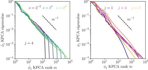
Figure 2: Convergence of spectra of activations $\hat{\phi}_{j}$ of finite-width trained scattering networks towards the feature vector $\phi_{j}$. The figure shows the covariance spectra of activations $\hat{\phi}_{j}$ for a given layer $j=4$ and various width scaling $s$ (left) and of the feature vector $\phi_{j}$ for the seven hidden layers $j\in\mathopen{}\mathclose{{}\left\{1,\dots,7}\right\}$ (right). The covariance spectrum is a power law of index close to $-1$.

We train several networks with a range of widths by simultaneously scaling the widths of all layers with a multiplicative factor $s$ varying over a range of $2^{6}=64$. We show that their activations $\hat{\phi}_{j}$ converge after alignment to a fixed deterministic limit $\phi_{j}$ when the width increases. The feature map $\phi_{j}$ is approximated with the activations of a large network with $s=2^{3}$.

We begin illustrating the behavior of activation spectra as a function of our width-scaling parameter $s$, for seven-hidden-layer trained scattering networks on CIFAR-10. In the left panel of Figure 2, we show how activation spectra vary as a function of $s$ for the layer $j=4$ which has a behavior representative of all other layers. The spectra are obtained by doing a PCA of the activations $\hat{\phi}_{j}(x)$, which corresponds to a KPCA of the input $x$ with respect to the empirical kernel $\hat{k}_{j}$. The $\hat{\phi}_{j}$ covariance spectra for networks of various widths overlap at lower KPCA ranks, suggesting well-estimated components, while the variance then decays rapidly at higher ranks. Wider networks thus estimate a larger number of principal components of the feature vector $\phi_{j}$. For the first layer $j=1$, this recovers the random feature KPCA results of Sriperumbudur and Sterge (2022), but this convergence is observed at all layers. The overall trend as a function of $s$ illustrates the infinite-width convergence. We also note that, as the width increases, the activation spectrum becomes closer to a power-law distribution with a slope of $-1$. The right panel of the figure shows that this type of decay with KPCA rank $m$ is observed at all layers of the infinite-width network $(\phi_{j})_{j\leq J}$. The power-law spectral properties of random feature activations have been studied theoretically by Scetbon and Harchaoui (2021), and in connection with the scaling laws observed in large language models (Kaplan et al., 2020) by Maloney et al. (2022). Note that here we do not scale the dataset size nor training hyperparameters such as the learning rate or batch size with the network width, and a different experimental setup would likely influence the infinite-width limit (Yang et al., 2022; Hoffmann et al., 2022).

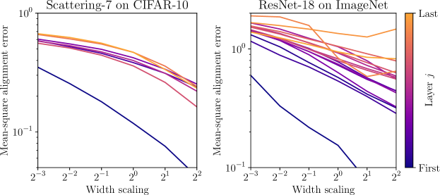
Figure 3: Convergence of activations $\hat{\phi}_{j}$ of finite-width networks towards the corresponding feature vector $\phi_{j}$, for scattering networks trained on CIFAR-10 (left) and ResNet trained on ImageNet (right). Both panels show the relative mean squared error $\mathbb{E}_{x}[{\lVert\hat{A}_{j}\,\hat{\phi}_{j}(x)-\phi_{j}(x)\rVert}{}^{2}]/\mathbb{E}_{x}[{\lVert\phi_{j}(x)\rVert}^{2}]$ between aligned activations $\hat{A}_{j}\,\hat{\phi}_{j}$ and the feature vector $\phi_{j}$. The error decreases as a function of the width scaling $s$ for all layers for the scattering network, and all but the last few layers for ResNet.

We now directly measure the convergence of activations by evaluating the mean-square distance after alignment $\mathbb{E}_{x}[{\lVert\hat{A}_{j}\,\hat{\phi}_{j}(x)-\phi_{j}(x)\rVert}{}^{2}]$. The left panel of Figure 3 shows that it does indeed decrease when the network width increases, for all layers $j$. Despite the theoretical convergence rate of Theorem  vanishing when the activation spectrum exponent $\alpha_{j}$ approaches $1$, in practice we still observe convergence. Alignment rotations $\hat{A}_{j}$ are computed on the train set while the mean-square distance is computed on the test set, so this decrease is not a result of overfitting. It demonstrates that scattering networks $\hat{\phi}_{j}$ approximate the same deterministic network $\phi_{j}$ no matter their initialization or width when it is large enough. The right panel of the figure evaluates this same convergence on a ResNet-18 trained on ImageNet. The mean-square distance after alignment decreases for most layers when the width increases. We note that the rate of decrease slows down for the last few layers. For these layers, the relative error after alignment is of the order of unity, indicating that the convergence is not observed at the largest width considered here. The overall trend however suggests that further increasing the width would reduce the error after alignment. The observations that networks trained from different initializations have similar activations had already been made by Raghu et al. (2017). Kornblith et al. (2019) showed that similarity increases with width, but with a weaker similarity measure. Rainbow networks, which we will show can approximate scattering networks, explain the source of these observations as a consequence of the law of large numbers applied to the random weight matrices with conditionally i.i.d. rows.

3.2 Properties of learned weight covariances

We have established the convergence (up to rotations) of the activations $\hat{\phi}_{j}$ in the infinite-width limit. Under the rainbow model, the weight matrices $W_{j}$ are random and thus cannot converge. However, they define estimates $\tilde{C}_{j}$ of the infinite-dimensional weight covariances $C_{j}$. We show that these estimates $\tilde{C}_{j}$ converge to the true covariances $C_{j}$ when the width increases. We then demonstrate that the covariances $C_{j}$ are effectively low-rank, and that their eigenspaces can be efficiently approximated by taking into account unsupervised information. The weight covariances are thus of low complexity, in the sense that they can be described with a number of parameters significantly smaller than their original size.

Estimation of the weight covariances.

We estimate the weight covariances $C_{j}$ from the learned weights of a deep network. This network has weight matrices $W_{j}$ of size $d_{j}\times d_{j-1}$ that have been trained end-to-end by SGD. The natural empirical estimate of the weight covariance $\hat{C}_{j}$ of $W_{j}$ is

$$\hat{C}_{j}\approx d_{j}^{-1}\,W_{j}^{\mathrm{T}}W_{j}.$$ (14)

It computes $\hat{C}_{j}$ from $d_{j}$ samples, which are conditionally i.i.d. under the rainbow model hypothesis. Although the number $d_{j}$ of samples is large, their dimension $d_{j-1}$ is also large. For many architectures $d_{j}/d_{j-1}$ remains nearly constant and we shall consider in this section that $d_{j}=s\,d_{j}^{0}$, so that when the scaling factor $s$ grows to infinity $d_{j}/d_{j-1}$ converges to a non-zero finite limit. This creates challenges in the estimation of $\hat{C}_{j}$, as we now explain. We will see that the weight variance is amplified during training. The learned covariance can thus be modeled $\hat{C}_{j}=\mathrm{Id}+\hat{C}^{\prime}_{j}$, where the magnitude of $\hat{C}^{\prime}_{j}$ keeps increasing during training. When the training time goes to infinity, the initialization $\mathrm{Id}$ becomes negligible with respect to $\hat{C}^{\prime}_{j}$. However, at finite training time, only the eigenvectors of $C^{\prime}_{j}$ with sufficiently high eigenvalues have been learned consistently, and $\hat{C}^{\prime}_{j}$ is thus effectively low-rank. $\hat{C}_{j}$ is then a spiked covariance matrix (Johnstone, 2001). A large statistical literature has addressed the estimation of spiked covariances when the number of parameters $d_{j-1}$ and the number of observations $d_{j}$ increases, with a constant ratio $d_{j}/d_{j-1}$ (Baik et al., 2005; El Karoui, 2008a). Consistent estimators of the eigenvalues of $\hat{C}_{j}$ can be computed, but not of its eigenvectors, unless we have other prior information such as sparsity of the covariance entries (El Karoui, 2008b) or its eigenvectors (Ma, 2013). In our setting, we shall see that prior information on eigenspaces of $\hat{C}_{j}$ is available from the eigenspaces of the input activation covariances. We use the empirical estimator (14) for simplicity, but it is not optimal. Minimax-optimal estimators are obtained by shrinking empirical eigenvalues (Donoho et al., 2018).

We would like to estimate the infinite-dimensional covariances $C_{j}$ rather than finite-dimensional projections $\hat{C}_{j}$. Since $\hat{C}_{j}=\hat{A}_{j-1}^{\mathrm{T}}C_{j}\hat{A}_{j-1}$, an empirical estimate of $C_{j}$ is given by

$$\tilde{C}_{j}=\hat{A}_{j-1}\hat{C}_{j}\hat{A}_{j-1}^{\mathrm{T}}.$$ (15)

To compute the alignment rotation $\hat{A}_{j-1}$ with eq. 4, we must estimate the infinite-width rainbow activations $\phi_{j-1}$. As above, we approximate $\phi_{j-1}$ with the activations $\hat{\phi}_{j-1}$ of a finite but sufficiently large network, relying on the activation convergence demonstrated in the previous section. We then estimate $C_{j}$ with eq. 15 and $\hat{C}_{j}\approx d_{j}^{-1}\,W_{j}^{\mathrm{T}}W_{j}$. We further reduce the estimation error of $C_{j}$ by training several networks of size $(d_{j})_{j\leq J}$, and by averaging the empirical estimators (15). Note that averaging directly the estimates (14) of $\hat{C}_{j}$ with different networks would not lead to an estimate of $C_{j}$, because the covariances $\hat{C}_{j}$ are represented in different bases which must be aligned. The final layer weights $\theta$ are also similarly computed with an empirical estimator from the trained weights $\hat{\theta}$.

Convergence of weight covariances.

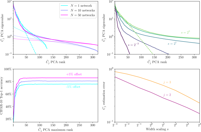
Figure 4: The weight covariance estimate $\tilde{C}_{j}$ converges towards the infinite-dimensional covariance $C_{j}$ for a three-hidden-layer scattering network trained on CIFAR-10. The first three panels show the behavior of the layer $j=2$. Upper left: spectra of empirical weight covariances $\tilde{C}_{j}$ as a function of the network sample size $N$ showing the transition from an exponential decay (fitted by the dashed line for $N=1$) to the Marchenko-Pastur spectrum (fitted by the dotted lines). Lower left: test classification performance on CIFAR-10 of the trained networks as a function of the maximum rank of its weight covariance $\tilde{C}_{j}$. Most of the performance is captured with the first eigenvectors of $\tilde{C}_{j}$. The curves for different network sample sizes $N$ when estimating $\tilde{C}_{j}$ overlap and are offset for visual purposes. Upper right: spectrum of empirical weight covariances $\tilde{C}_{j}$ as a function of the network width scaling $s$. The dashed line is a fit to an exponential decay at low rank. Lower right: relative distance between empirical and true covariances ${\lVert\hat{C}_{j}-C_{j}\rVert}{}_{\infty}/{\lVert C_{j}\rVert}{}_{\infty}$, as a function of the width scaling $s$.

We now show numerically that the weight covariance estimates $\tilde{C}_{j}$ (15) converge to the true covariances $C_{j}$. This performs a partial validation of the rainbow assumptions of Definition , as it verifies the rotation of the second-order moments of $\pi_{j}$ (12) but not higher-moments nor independence between neurons. Due to computational limitations, we perform this verification on three-hidden-layer scattering networks trained on CIFAR-10, for which we can scale both the number of networks $N$ we can average over, and their width $s$. The main computational bottleneck here is the singular value decomposition of the cross-covariance matrix $\mathbb{E}_{x}[\phi_{j}(x)\,\hat{\phi}_{j}(x)^{\mathrm{T}}]$ to compute the alignment $\hat{A}_{j}$, which requires $O(Ns^{3})$ time and $O(Ns^{2})$ memory. These shallower networks reach a test accuracy of $84\%$ at large width.

We begin by showing that empirical covariance matrices $\tilde{C}_{j}$ estimated from the weights of different networks share the same eigenspaces of large eigenvalues. To this end, we train $N$ networks of the same finite width ($s=1$) and compare the covariances $\tilde{C}_{j}$ estimated from these $N$ networks as a function of $N$. As introduced above, the estimated covariances $\tilde{C}_{j}$ are well modeled with a spiked-covariance model. The upper-left panel of Figure 4 indeed shows that the covariance spectrum interpolates between an exponential decay at low ranks (indicated by the dashed line, corresponding to the “spikes” resulting from training, as will be shown in Section 3.3), and a Marchenko-Pastur tail at higher ranks (indicated by dotted lines, corresponding to the initialization with identity covariance). Note that we show the eigenvalues as a function of their rank rather than a spectral density in order to reveal the exponential decay of the spike positions with rank, which was missed in previous works (Martin and Mahoney, 2021; Thamm et al., 2022). The exponential regime is present even in the covariance estimated from a single network, indicating its stability across training runs, while the Marchenko-Pastur tail becomes flatter as more samples are used to estimate the empirical covariance. Here, the feature vector $\phi_{j}$ has been estimated with a scattering network of same width $s=1$ for simplicity of illustration.

As shown in the lower-left panel, only the exponential regime contributes to the classification accuracy of the network: the neuron weights can be projected on the first principal components of $\tilde{C}_{j}$, which correspond to the learned spikes, without harming performance. The informative component of the weights is thus much lower-dimensional ($\approx 30$) than the network width ($128$), and this dimension appears to match the characteristic scale of the exponential decay of the covariance eigenvalues. The number $N$ of trained networks used to compute $\tilde{C}_{j}$ has no appreciable effect on the approximation accuracy, which again shows that the empirical covariance matrices of all $N$ networks share this common informative component. This presence of a low-dimensional informative weight component is in agreement with the observation that the Hessian of the loss at the end of training is dominated by a subset of its eigenvectors (LeCun et al., 1989b; Hassibi and Stork, 1992). These Hessian eigenvectors could indeed be related to the weight covariance eigenvectors. Similarly, the dichotomy in weight properties highlighted by our analysis could indicate why the eigenvalue distribution of the loss Hessian separates into two distinct regimes (Sagun et al., 2016, 2017; Papyan, 2019): the “bulk” (with small eigenvalues corresponding to uninformative flat directions of the loss landscape) is related to the Marchenko-Pastur tail of our weight covariance spectrum and the “top” (or spiked) components correspond to the exponential regime found at the lowest ranks of the covariance spectrum.

We now demonstrate that the weight covariances $\tilde{C}_{j}$ converge to an infinite-dimensional covariance operator $C_{j}$ when the widths of the scattering networks increase. Here, the weight covariances $\tilde{C}_{j}$ are estimated from the weights of $N=10$ networks with the same width scaling $s$, and we estimate $C_{j}$ from the weights of $N=10$ wide scattering networks with $s=2^{5}$. We first illustrate this convergence on the spectrum of $\tilde{C}_{j}$ in the upper-right panel of Figure 2. The entire spectrum of $\tilde{C}_{j}$ converges to a limiting spectrum which contains both the informative exponential part resulting from training and the uninformative Marchenko-Pastur tail coming from the initialization. The characteristic scale of the exponential regime grows with network width but converges to a finite value as the width increases to infinity. We then confirm that the estimated covariances $\tilde{C}_{j}$ indeed converge to the covariance $C_{j}$ when the width increases in the lower-right panel. The distance converges to zero as a power law of the width scaling. The first layer $j=1$ has a different convergence behavior (not shown) as its input dimension does not increase with $s$.

In summary, in the context considered here, networks trained from different initializations share the same informative weight subspaces (after alignment) described by the weight covariances at each layer, and they converge to a deterministic limit when the width increases. The following paragraphs then demonstrate several properties of the weight covariances.

Dimensionality reduction in deep networks.

We now consider deeper networks and show that they also learn low-rank covariances. Comparing the spectra of weights and activations reveals the alternation between dimensionality reduction with the colored weight covariances $C_{j}$ and high-dimensional embeddings with the white random features which are captured in the rainbow model. We do so with two architectures: a ten-hidden-layer scattering network and a slightly modified ResNet-18 trained on ImageNet (specified in Appendix D), which both reach $89\%$ top-5 test accuracy.

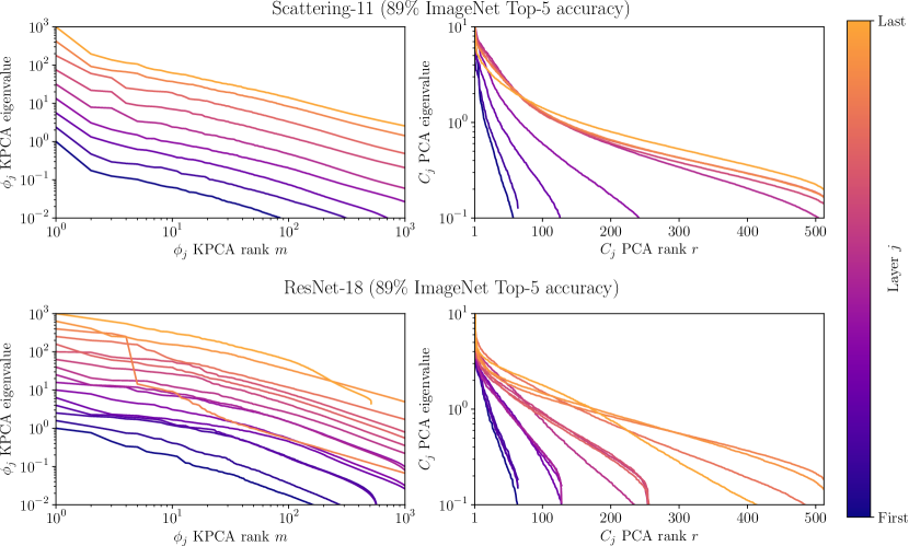
Figure 5: Covariance spectra of activations and weights of an ten-hidden-layer scattering network (top) and ResNet-18 (bottom) trained on ImageNet. In both cases, activation spectra (left) mainly follow power-law distribution with index roughly $-1$. Weight spectra (right) show a transition from an exponential decay with a characteristic scale increasing with depth to the Marchenko-Pastur spectral distribution. These behaviors are captured by the rainbow model. For visual purposes, activation and weight spectra are offset by a factor depending on $j$. In addition, we do not show the first layer nor the $1\times 1$ convolutional residual branches in ResNet as they have different layer properties.

We show the spectra of covariances of activations $\phi_{j}$ in the left panels of Figure 5 and of the weight covariances $C_{j}$ in the right panels. For both networks, we recover the trend that activation spectra are close to power laws of slope $-1$ and the weight spectra show a transition from a learned exponential regime to a decay consistent with the Marchenko-Pastur expectation, which is almost absent for ResNet-18. Considering them in sequence, as a function of depth, the input activations are thus high-dimensional (due to the power-law of index close to $-1$) while the subsequent weights perform a dimensionality reduction using an exponential bottleneck with a characteristic scale much smaller than the width. Next, the dimensionality is re-expanded with the non-linearity, as the activations at the next layer again have a power-law covariance spectrum. Considering the weight spectra, we observe that the effective exponential scale increases with depth, from about $10$ to $60$ for both the scattering network and the ResNet. This increase of dimensionality with depth is expected: in convolutional architectures, the weight covariances $C_{j}$ are only defined on small patches of activations $\phi_{j-1}$ because of the prior operator $P_{j}$. However, these patches correspond to a larger receptive field in the input image $x$ as the depth $j$ increases. The rank of the covariances is thus to be compared with the size of this receptive field. Deep convolutional networks thus implement a sequence of dimensionality contractions (with the learned weight covariances) and expansions (with the white random features and non-linearity). Without the expansion, the network would reduce the dimensionality of the data exponentially fast with depth, thus severely limiting its ability to process information on larger spatial scales (deeper layers), while without the contraction, its parameter count and learning sample complexity would increase exponentially fast with depth. This contraction/expansion strategy allows the network to maintain a balanced representation at each scale.

The successive increases and decreases in dimensionality due to the weights and non-linearity across deep network layers have been observed by Recanatesi et al. (2019) with a different dimensionality measure. The observation that weight matrices of trained networks are low-rank has been made in several works which exploited it for model compression (Denil et al., 2013; Denton et al., 2014; Yu et al., 2017), while the high-dimensional embedding property of random feature maps is well-known via the connection to their kernel (Rahimi and Recht, 2007; Scetbon and Harchaoui, 2021). The rainbow model integrates these two properties. In neuroscience, high-dimensional representations with power-law spectra have been measured in the mouse visual cortex by Stringer et al. (2019). Such representations in deep networks have been demonstrated to lead to increased predictive power of human fMRI cortical responses (Elmoznino and Bonner, 2022) and generalization in self-supervised learning (Agrawal et al., 2022).

Unsupervised approximations of weight covariances.

The learning complexity of a rainbow network depends upon the number of parameters needed to specify the weight covariances $(C_{j})_{j\leq J}$ to reach a given performance. After having shown that their informative subspace is of dimension significantly lower than the network width, we now show that this subspace can be efficiently approximated by taking into account unsupervised information.

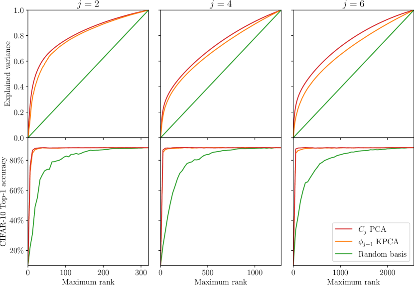
Figure 6: Unsupervised information defines low-dimensional approximations of the learned weight covariances. Each column shows a different layer $j=2,\,4,\,6$ of a seven-hidden-layer scattering network trained on CIFAR-10. For each $r$, we consider projections of the network weights on the first $r$ principal components of the weight covariances (red), the kernel principal components of the input activations (orange), or random orthogonal vectors (green). Top: weight variance explained by the first $r$ basis vectors as a function of $r$. Bottom: classification accuracy after projection of the $j$-th layer weights on the first $r$ basis vectors, as function of $r$.

We would like to define a representation of the weight covariances $C_{j}$ which can be accurately approximated with a limited number of parameters. We chose to represent the infinite-width activations $\phi_{j}$ as KPCA feature vectors, whose uncentered covariances $\mathbb{E}_{x}[\phi_{j}(x)\,\phi_{j}(x)^{\mathrm{T}}]$ are diagonal. In that case, the weight covariances $C_{j}$ for $j>1$ are operators defined on $H_{j-1}=\ell^{2}(\mathbb{N})$. It amounts to representing $C_{j}$ relatively to the principal components of $\phi_{j-1}$, or equivalently, the kernel principal components of $x$ with respect to $k_{j-1}$. This defines unsupervised approximations of the weight covariance $C_{j}$ by considering its projection on these first principal components. We now evaluate the quality of this approximation.

Here, we consider a seven-hidden-layer scattering network trained on CIFAR-10, and weight covariances estimated from $N=50$ same-width networks. The upper panels of Figure 6 shows the amount of variance in $C_{j}$ captured by the first $m$ basis directions as a function of $m$, for three different orthogonal bases. The speed of growth of this variance as a function of $m$ defines the quality of the approximation: a faster growth indicates that the basis provides an efficient low-dimensional approximation of the covariance. The PCA basis of $C_{j}$ provides optimal such approximations, but it is not known before supervised training. In contrast, the KPCA basis is computed from the previous layer activations $\phi_{j-1}$ without the supervision of class label information. Figure 6 demonstrates that the $\phi_{j-1}$ KPCA basis provides close to optimal approximations of $C_{j}$. This approximation is more effective for earlier layers, indicating that the supervised information becomes more important for the deeper layers. The lower panels of Figure 6 show a similar phenomenon when measuring classification accuracy instead of weight variance.

In summary, the learned weight matrices are low-rank, and a low-dimensional bottleneck can be introduced without harming performance. Further, unsupervised information (in the form of a KPCA) gives substantial prior information on this bottleneck: high-variance components of the weights are correlated with high-variance components of the activations. This observation was indirectly made by Raghu et al. (2017), who showed that network activations can be projected on stable subspaces, which are in fact aligned with the high-variance kernel principal components. It demonstrates the importance of self-supervised learning within supervised learning tasks (Bengio, 2012), and corroborates the empirical success of self-supervised pre-training for many supervised tasks. The effective number of parameters that need to be learned in a supervised manner is thus much smaller than the total number of trainable parameters.

3.3 Gaussian rainbow approximations

We now show that the Gaussian rainbow model applies to scattering networks trained on the CIFAR-10 dataset, by exploiting the fixed wavelet spatial filters incorporated in the architecture. The Gaussian assumption thus only applies to weights along channels. We make use of the factorization $W_{j}=G_{j}\,\hat{C}_{j}^{1/2}$ (13) of trained weights, where $\hat{C}_{j}$ results from an estimation of $C_{j}$ from several trained networks. We first show that the distribution of $G_{j}$ can be approximated with random matrices of i.i.d. normal coefficients. We then show that Gaussian rainbow networks, which replace $G_{j}$ with such a white Gaussian matrix, achieve similar classification accuracy as trained networks when the width is large. Finally, we show that in the same context, the SGD training dynamics of the weight matrices $W_{j}$ are characterized by the evolution of the weight covariances $\hat{C}_{j}$ only, while $G_{j}$ remains close to its initial value. The Gaussian approximation deteriorates at small widths or on more complex datasets, suggesting that its validity regime is when the network width is large compared to the task complexity.

Comparison between trained weights and Gaussian matrices.

We show that statistics of trained weights are reasonably well approximated by the Gaussian rainbow model. To do so, we train $N=50$ seven-hidden-layer scattering networks and estimate weight covariances $(C_{j})_{j\leq J}$ by averaging eq. 15 over the trained networks as explained in Section 3.2. We then retrieve $G_{j}=W_{j}\,\hat{C}_{j}^{-1/2}$ with $\hat{C}_{j}=\hat{A}_{j}^{\mathrm{T}}C_{j}\hat{A}_{j}$ as in eq. 12. Note that we use a single covariance $C_{j}$ to whiten the weights of all $N$ networks: this will confirm that the covariances of weights of different networks are indeed related through rotations, as was shown in Section 3.2 through the convergence of weight covariance estimates. The rainbow feature vectors $(\phi_{j})_{j\leq J}$ at each layer are approximated with the activations of one of the $N$ networks.

Figure 7: Marginal distributions of the weights of $N=50$ seven-hidden-layer scattering networks trained on CIFAR-10. The weights at the $j$-th layer $(w_{ji})_{i\leq d_{j}}$ of the $N$ networks are projected along the $r$-th eigenvector of $C_{j}$ and normalized by the square root of the corresponding eigenvalue. The distribution of the $Nd_{j}$ projections (blue histograms) is approximately normal (red curves). Each column shows a different layer $j$, and each row shows a different rank $r$.

As a first (partial) Gaussianity test, we compare marginal distributions of whitened weights $G_{j}$ with the expected normal distribution in Figure 7. We present results for a series of layers ($j=2,4,6$) across the network. Other layers present similar results, except for $j=1$ which has more significant deviations from Gaussianity (not shown), as its input dimension is constrained by the data dimension. We shall however not focus on this first layer as we will see that it can still be replaced by Gaussian realizations when generating new weights. The weights at the $j$-th layer $(w_{ji})_{i\leq d_{j}}$ of the $N$ networks are projected along the $r$-th eigenvector of $C_{j}$ and normalized by the square root of the corresponding eigenvalue. This global view shows that specific one-dimensional marginals are reasonably well approximated by a normal distribution. We purposefully remain not quantitative, as the goal is not to demonstrate that trained weights are statistically indistinguishable from Gaussian realizations (which is false), but to argue that the latter is an acceptable model for the former.

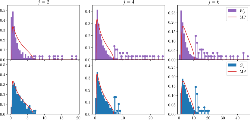
Figure 8: Spectral density of empirical covariances of trained (top) and whitened weights (bottom). Eigenvalue outside the support of the Marchenko-Pastur distribution (shown in red) are indicated with spikes of amplitude proportional to their bin count. After whitening, the number of outliers are respectively $2\%$, $4\%$, and $8\%$ for the layers $j=2$, $4$, and $6$.

To go beyond one-dimensional marginals, we now compare in the bottom panels of Figure 8 the spectral density of the whitened weights $G_{j}$ to the theoretical Marchenko-Pastur distribution (Marčenko and Pastur, 1967), which describes the limiting spectral density of matrices with i.i.d. normal entries. We note a good agreement for the earlier layers, which deteriorates for deeper layers (as well as the first layer, not shown, which again has a different behavior). Importantly, the proportion of eigenvalues outside the Marchenko-Pastur support is arguably negligible ($<10\%$ at all layers), which is not the case for the non-whitened weights $W_{j}$ (upper panels) where it can be $>25\%$ for $j=6$. As observed by Martin and Mahoney (2021) and Thamm et al. (2022), trained weights have non-Marchenko-Pastur spectral statistics. Our results show that these deviations are primarily attributable to correlations introduced by the non-identity covariance matrices $C_{j}$, as opposed to power-law distributions as hypothesized by Martin and Mahoney (2021). We however note that due to the universality of the Marchenko-Pastur distribution, even a perfect agreement is not sufficient to claim that trained networks have conditionally Gaussian weights. It merely implies that the Gaussian rainbow model provides a satisfactory description of a number of weight statistical properties. Despite the observed deviations from Gaussianity at later layers, we now show that generating new Gaussian weights at all layers simultaneously preserves most of the classification accuracy of the network.

Performance of Gaussian rainbow networks.

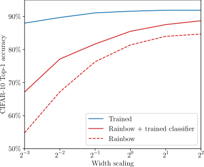
Figure 9: Performance of seven-hidden-layer scattering networks on CIFAR-10 as a function of network width for a trained network (blue), its rainbow network approximation with and without classifier retraining (red solid and dashed). The larger the width, the better the sampled rainbow model approximates the original network.

While the above tests indicate some level of validation that the whitened weights $G_{j}$ are matrices with approximately i.i.d. normal entries, it is not statistically feasible to demonstrate that this property is fully satisfied in high-dimensions. We thus sample network weights from the Gaussian rainbow model and verify that most of the performance can be recovered. This is done with the procedure described in Definition , using the covariances $C_{j}$, rainbow activations $\phi_{j}$ and final layer weights $\theta$ here estimated from a single trained network (having shown in Sections 3.1 and 3.2 that all networks define similar rainbow parameters if they are wide enough). New weights $W_{j}$ are sampled iteratively starting from the first layer with a covariance $\hat{C}_{j}=\hat{A}_{j-1}^{\mathrm{T}}C_{j}\hat{A}_{j-1}$, after computing the alignment rotation $\hat{A}_{j-1}$ between the activations $\hat{\phi}_{j-1}(x)$ of the partially sampled network and the activations $\phi_{j-1}(x)$ of the trained network. The alignment rotations are computed using the CIFAR-10 train set, while network accuracy is evaluated on the test set, so that the measured performance is not a result of overfitting.

We perform this test using a series of seven-hidden-layer scattering networks trained on CIFAR-10 with various width scalings. We present results in Figure 9 for two sets of Gaussian rainbow networks: a first set for which both the convolutional layers and the final layer are sampled from the rainbow model (which corresponds to aligning the classifier of the trained model to the sampled activations $\hat{\phi}_{J}(x)$), and another set for which we retrain the classifier after sampling the convolutional layers (which preserves the Gaussian rainbow RKHS). We observe that the larger the network, the better it can be approximated by a Gaussian rainbow model. At the largest width considered here, the Gaussian rainbow network achieves $85\%$ accuracy and $89\%$ with a retrained classifier, and recovers most of the performance of the trained network which reaches $92\%$ accuracy. This performance is non-trivial, as it is beyond most methods based on non-learned hierarchical convolutional kernels which obtain less than $83\%$ accuracy (Mairal et al., 2014; Oyallon and Mallat, 2015; Li et al., 2019). This demonstrates the importance of the learned weight covariances $C_{j}$, as has been observed by Pandey et al. (2022) for modeling sensory neuron receptive fields. It also demonstrates that the covariances $C_{j}$ are sufficiently well-estimated from a single network to preserve classification accuracy. We note however that Shankar et al. (2020) achieve a classification accuracy of $90\%$ with a non-trained kernel corresponding to an infinite-width convolutional network.

A consequence of our results is that these trained scattering networks have rotation invariant non-linearities, in the sense that the non-linearity can be applied in random directions, provided that the next layer is properly aligned. This comes in contrast to the idea that neuron weights individually converge to salient features of the input data. For large enough networks, the relevant information learned at the end of training is therefore not carried by individual neurons but encoded through the weight covariances $C_{j}$.

For smaller networks, the covariance-encoding property no longer holds, as Figure 9 suggests that trained weights becomes non-Gaussian. Networks trained on more complex tasks might require larger widths for the Gaussian rainbow approximation to be valid. We have repeated the analysis on scattering networks trained on the ImageNet dataset (Russakovsky et al., 2015), which reveals that the Gaussian rainbow approximation considered here is inadequate at widths used in practice. This is corroborated by many empirical observations of (occasional) semantic specialization in deep networks trained on ImageNet (Olah et al., 2017; Bau et al., 2020; Dobs et al., 2022). A promising direction is to consider Gaussian mixture rainbow models, as used by Dubreuil et al. (2022) to model the weights of linear RNNs. Finally, we note that the Gaussian approximation also critically rely on the fixed wavelet spatial filters of scattering networks. Indeed, the spatial filters learned by standard CNNs display frequency and orientation selectivity (Krizhevsky et al., 2012) which cannot be achieved with a single Gaussian distribution, and thus require adapted weight distributions $\pi_{j}$ to be captured in a rainbow model.

Training dynamics.

The rainbow model is a static model, which does not characterize the evolution of weights from their initialization during training. We now describe the SGD training dynamics of the seven-hidden-layer scattering network trained on CIFAR-10 considered above. This dynamic picture provides an empirical explanation for the validity of the Gaussian rainbow approximation.

We focus on the $j$-th layer weight matrix $W_{j}(t)$ as the training time $t$ evolves. To measure its evolution, we consider its projection along the principal components of the final learned covariance $\hat{C}_{j}$. More precisely, we project the $d_{j}$ neuron weights $w_{ji}(t)$, which are the rows of $W_{j}(t)$, in the direction of the $r$-th principal axis $e_{jr}$ of $\hat{C}_{j}$. This gives a vector $u_{r}(t)\in\mathbb{R}^{d_{j}}$ for each PCA rank $r$ and training time $t$, dropping the index $j$ for simplicity:

$$u_{r}(t)=\mathopen{}\mathclose{{}\left(\langle w_{ji}(t),e_{jr}\rangle}\right)_{i\leq d_{j}}.$$

Its squared magnitude is proportional to the variance of the neuron weights along the $r$-th principal direction, which should be of the order of $1$ at $t=0$ due to the white noise initialization, and evolves during training to reach the corresponding $\hat{C}_{j}$ eigenvalue. On the opposite, the direction of $u_{r}(t)$ encodes the sampling of the marginal distribution of the neurons along the $r$-th principal direction: a large entry $u_{r}(t)[i]$ indicates that neuron $i$ is significantly correlated with the $r$-th principal component of $\hat{C}_{j}$. This view allows considering the evolution of the weights $W_{j}(t)$ separately for each principal component $r$. It offers a simpler view than focusing on each individual neuron $i$, because it gives an account of the population dynamics across neurons. It separates the weight matrix by columns $r$ (in the weight PCA basis) rather than rows $i$. We emphasize that we consider the PCA basis of the final covariance $\hat{C}_{j}$, so that we analyze the training dynamics along the fixed principal axes $e_{jr}$ which do not depend on the training time $t$.

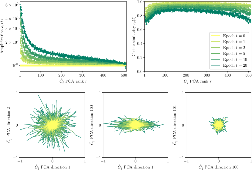
Figure 10: The learning dynamic of a seven-hidden-layer scattering network trained on CIFAR-10 is mainly a low-dimensional linear amplification effect that preserves most of the positional information of the initialization. We present results for layer $j=4$ (similar behavior is observed for the other layers). Upper left: amplification (overall stretch) of the weight variance as a function of rank. Upper right: cosine similarity (internal motion) as a function of rank. Lower panels: projections of individual neurons along pairs of principal components. Each neuron is represented as a point in the plane, whose trajectory during training is shown as a connected line (color indicates training time).

We now characterize the evolution of $u_{r}(t)$ during training for each rank $r$. We separate changes in magnitude, which correspond to changes in weight variance (overall stretch), from changes in direction, which correspond to internal motions of the neurons which preserve their variance. We thus define two quantities to compare $u_{r}(t)$ to its initialization $u_{r}(0)$, namely the amplification ratio $a_{r}(t)$ and cosine similarity $c_{r}(t)$:

$$a_{r}(t)=\frac{{\lVert u_{r}(t)\rVert}}{{\lVert u_{r}(0)\rVert}}\leavevmode\nobreak\ \leavevmode\nobreak\ \text{and}\leavevmode\nobreak\ \leavevmode\nobreak\ c_{r}(t)=\frac{\langle u_{r}(t),u_{r}(0)\rangle}{{\lVert u_{r}(t)\rVert}\,{\lVert u_{r}(0)\rVert}}.$$ (16)

We evaluate these quantities using our seven-hidden-layer scattering network trained on CIFAR-10. In Figure 10, we present the results for the intermediate layer $j=4$ (similar behavior is observed for the other layers). We show the two quantities $a_{r}(t)$ and $c_{r}(t)$ in the top row of Figure 10 as a function of the training epoch $t$. We observe that the motion of the weight vector is mainly an amplification effect operating in a sequence starting with the first eigenvectors, as the cosine similarity remains of order unity. Given the considered dimensionality ($d_{j}=512$), the observed departure from unity is rather small: the solid angle subtended by this angular change of direction covers a vanishingly small surface of the unit sphere in $d_{j}$ dimensions. We thus have $u_{r}(t)\approx a_{r}(t)\,u_{r}(0)$.

These results show that the weight evolution can be written

$$W_{j}(t)\approx G_{j}\,\hat{C}_{j}^{1/2}(t),$$

where $G_{j}=W_{j}(0)$ is the initialization and the weight covariance $\hat{C}_{j}(t)$ evolves by amplification in its fixed PCA basis:

$$\hat{C}_{j}(t)=\sum_{r}a_{r}(t)^{2}\,e_{jr}e_{jr}^{\mathrm{T}}.$$

In other words, the weight evolution during training is an ensemble motion of the neuron population, with negligible internal motion of individual neurons relative to the population: training amounts to learning the weight covariance. Surprisingly, the weight configuration at the end of training thus retains most of the information of its random initialization: the initial configuration can be practically recovered by whitening the trained weights. In addition, the stochasticity introduced by SGD and data augmentation appears to be negligible, as it does not affect the relative positions of individual neurons during training. This observation has two implications. First, the alignment rotations $\hat{A}_{j}$ which describe the trained network relative to its infinite-width rainbow counterpart (as $\hat{\phi}_{j}\approx\hat{A}_{j}^{\mathrm{T}}\phi_{j}$) are entirely determined by the initialization. Second, it provides an empirical explanation for the validity of the Gaussian rainbow approximation. While this argument seems to imply that the learned weight distributions $\pi_{j}$ depend significantly on the initialization scheme, note that significantly non-Gaussian initializations might not be preserved by SGD or could lead to poor performance.

The bottom row of Figure 10 illustrates more directly the evolution of individual neurons during training. Although each neuron of $W_{j}(t)$ is described by a $d_{j-1}$-dimensional weight vector, it can be projected along two principal directions to obtain a two-dimensional picture. We then visualize the trajectories of each neuron projected in this plane. The trajectories are almost straight lines, as the learning dynamics only amplify variance along the principal directions while preserving the relative positions of the neurons. Projections on principal components of higher ranks give a more static picture as the amplification along these directions is smaller.

A large literature has characterized properties of SGD training dynamics. Several works have observed that dynamics are linearized after a few epochs (Jastrzebski et al., 2020; Leclerc and Madry, 2020), so that the weights remain in the same linearly connected basin thereafter (Frankle et al., 2020). It has also been shown that the empirical neural tangent kernel evolves mostly during this short initial phase (Fort et al., 2020) and aligns itself with discriminative directions (Baratin et al., 2021; Atanasov et al., 2022). Our results indicate that this change in the neural tangent kernel is due to the large amplification of the neuron weights along the principal axes of $\hat{C}_{j}$, which happen early during training. The observation that neural network weights have a low-rank departure from initialization has been made in the lazy regime by Thamm et al. (2022), for linear RNNs by Schuessler et al. (2020), and for large language-model adaptation by Hu et al. (2022). The sequential emergence of the weight principal components has been derived theoretically in linear networks by Saxe et al. (2014, 2019).

4 Conclusion

We have introduced rainbow networks as a model of the probability distribution of weights of trained deep networks. The rainbow model relies on two assumptions. First, layer dependencies are reduced to alignment rotations. Second, neurons are independent when conditioned on the previous layer weights. Under these assumptions, trained networks converge to a deterministic function in the corresponding rainbow RKHS when the layer widths increase. We have verified numerically the convergence of activations after alignment for scattering networks and ResNets trained on CIFAR-10 and ImageNet. We conjecture that this convergence conversely implies the rotation dependency assumption of the rainbow model. We have verified this rotation on the second-order moments of the weights through the convergence of their covariance after alignment (for scattering networks trained on CIFAR-10 due to computational limitations).

The data-dependent kernels which describe the infinite-width rainbow networks, and thus their functional properties, are determined by the learned distributions $\pi_{j}$. Mathematically, we have shown how the symmetry properties of these distributions are transferred on the network. Numerically, we have shown that their covariances $C_{j}$ compute projections in a low-dimensional “informative” subspace that is shared among networks, is low-dimensional, and can be approximated efficiently with an unsupervised KPCA. It reveals that networks balance low learning complexity with high expressivity by computing a sequence of reductions and increases in dimensionality.

In the Gaussian case, the distributions $\pi_{j}$ are determined by their covariances $C_{j}$. We have validated that factorizing the learned weights with fixed wavelet filters is sufficient to obtain Gaussian rainbow networks on CIFAR-10, using scattering networks. In this setting, we can generate new weights and have shown that the weight covariances $C_{j}$ are sufficient to capture most of the performance of the trained networks. Further, the training dynamics are reduced to learning these covariances while preserving memory of the initialization in the individual neuron weights.

Our work has several limitations. First, we have not verified the rainbow assumptions of rotation dependence between layers beyond second-order moments, and conditional independence between neurons beyond the Gaussian case. A complete model would incorporate the training dynamics and show that such statistical properties are satisfied at all times. Second, our numerical experiments have shown that the Gaussian rainbow approximation of scattering networks gradually degrades when the network width is reduced. When this approximation becomes less accurate, it raises the question whether incorporating more prior information in the architecture could lead to Gaussian rainbow networks. Finally, even in the Gaussian case, the rainbow model is not completely specified as it requires to estimate the weight covariances $C_{j}$ from trained weights. A major mathematical issue is to understand the properties of the resulting rainbow RKHS which result from properties of these weight covariances.

By introducing the rainbow model, this work provides new insights towards understanding the inner workings of deep networks.

Acknowledgments

This work was partially supported by a grant from the PRAIRIE 3IA Institute of the French ANR-19-P3IA-0001 program. BM acknowledges support from the David and Lucile Packard Foundation. We thank the Scientific Computing Core at the Flatiron Institute for the use of their computing resources. BM thanks Chris Olah and Eric Vanden-Eijnden for inspiring discussions. FG would like to thank Francis Bach and Gabriel Peyré for helpful pointers for the proof of Theorem . We also thank Nathanaël Cuvelle-Magar and Etienne Lempereur for feedback on the manuscript.

Appendix A Proof of Theorem 

We prove a slightly more general version of Theorem  which we will need in the proof of Theorem . We allow the input $x$ to be in a possibly infinite-dimensional Hilbert space $H_{0}$ (the finite-dimensional case is recovered with $H_{0}=\mathbb{R}^{d_{0}})$. We shall assume that the random feature distribution $\pi$ has bounded second- and fourth-order moments in the sense of Section 2.2: it admits a bounded uncentered covariance operator $C=\mathbb{E}_{w\sim\pi}[ww^{\mathrm{T}}]$ and $\mathbb{E}_{w\sim\pi}[(w^{\mathrm{T}}Tw)^{2}]<+\infty$ for every trace-class operator $T$ on $H_{0}$. Without loss of generality, we assume that the non-linearity $\rho$ is $1$-Lipschitz and that $\rho(0)=0$. These last assumptions simplify the constants involved in the analysis. They can be satisfied for any $L$-Lipschitz non-linearity $\rho$ by replacing it with $(\rho-\rho(0))/L$, which does not change the linear expressivity of the network.

We give the proof outline in Section A.1. It relies on several lemmas, which are proven in Sections A.2, A.3, A.4 and A.5. We write ${\mathopen{}\mathclose{{}\left\lVert\cdot}\right\rVert}_{\infty}$ the operator norm, ${\mathopen{}\mathclose{{}\left\lVert\cdot}\right\rVert}_{2}$ the Hilbert-Schmidt norm, and ${\mathopen{}\mathclose{{}\left\lVert\cdot}\right\rVert}_{1}$ the nuclear (or trace) norm.

A.1 Proof outline

The convergence of the activations $\hat{\varphi}(x)$ to the feature vector $\varphi(x)$ relies on the convergence of the empirical kernel $\hat{k}$ to the asymptotic kernel $k$. We thus begin by reformulating the mean-square error $\mathbb{E}_{x}[{\lVert\hat{A}\,\hat{\varphi}(x)-\varphi(x)\rVert}{}_{H}^{2}]$ in terms of the kernels $\hat{k}$ and $k$. More precisely, we will consider the integral operators $\hat{T}$ and $T$ associated to the kernels. These integral operators are the infinite-dimensional equivalent of Gram matrices $(k(x_{i},x_{i^{\prime}}))_{1\leq i,i^{\prime}\leq n}$.

Let $\mu$ be the distribution of $x$. We define the integral operator $T\colon L^{2}(\mu)\to L^{2}(\mu)$ associated to the asymptotic kernel $k$ as

$$\mathopen{}\mathclose{{}\left(Tf}\right)(x)=\mathbb{E}_{x^{\prime}}\mathopen{}\mathclose{{}\left[k(x,x^{\prime})\,f(x^{\prime})}\right],$$

where $x^{\prime}$ is an i.i.d. copy of $x$ and $\mu$ is the law of $x$. Similarly, we denote $\hat{T}$ the integral operator defined by $\hat{k}$. Their standard properties are detailed in the next lemma. Moreover, the definition of $\hat{T}$ entails that it is the average of $d_{1}$ i.i.d. integral operators defined by the individual random features $(w_{i})_{i\leq d_{1}}$ of $\hat{\varphi}$. The law of large numbers then implies a mean-square convergence of $\hat{T}$ to $T$, as proven in the following lemma.

Lemma 0

$T$ and $\hat{T}$ are trace-class non-negative self-adjoint operators on $L^{2}(\mu)$, with

$$\operatorname{tr}(T)\leq{\mathopen{}\mathclose{{}\left\lVert C}\right\rVert}_{\infty}\,\mathbb{E}_{x}[{\mathopen{}\mathclose{{}\left\lVert x}\right\rVert}^{2}].$$

The eigenvalues of $T$ and $\hat{T}$ are the same as their respective activation covariance matrices $\mathbb{E}_{x}[\varphi(x)\,\varphi(x)^{\mathrm{T}}]$ and $\mathbb{E}_{x}[\hat{\varphi}(x)\,\hat{\varphi}(x)^{\mathrm{T}}]$. Besides, it holds that $\mathbb{E}_{W}[\hat{T}]=T$ and

$$\sqrt{\mathbb{E}_{W}\mathopen{}\mathclose{{}\left[{\lVert\hat{T}-T\rVert}{}_{2}^{2}}\right]}=\sqrt{\mathbb{E}_{W,x,x^{\prime}}\mathopen{}\mathclose{{}\left[{\lvert\hat{k}(x,x^{\prime})-k(x,x^{\prime})\rvert}{}^{2}}\right]}=c\,d_{1}^{-1/2},$$

with some constant $c<+\infty$.

We defer the proof, which relies on standard properties and a direct calculation of the variance of $\hat{T}$ around its mean $T$, to Section A.2. In the following, we shall write $c=\kappa\,{\lVert C\rVert}_{\infty}\,\mathbb{E}_{x}[{\mathopen{}\mathclose{{}\left\lVert x}\right\rVert}^{2}]$ to simplify calculations for the proof of Theorem , where $C=\mathbb{E}_{w\sim\pi}[ww^{\mathrm{T}}]$ is the uncentered covariance of $\pi$, and $\kappa$ is a constant. When $\pi$ is Gaussian, Section A.2 further shows that $\kappa\leq\sqrt{3}$.

The mean-square error between $\hat{\varphi}$ and $\varphi$ after alignment can then be expressed as a different distance between $\hat{T}$ and $T$, as proven in the next lemma.

Lemma 0

The alignment error between $\hat{\varphi}$ and $\varphi$ is equal to the Bures-Wasserstein distance $\mathrm{BW}$ between $\hat{T}$ and $T$:

$$\min_{\hat{A}\in\mathcal{O}\mathopen{}\mathclose{{}\left(d_{1}}\right)}\mathbb{E}_{x}\mathopen{}\mathclose{{}\left[{\lVert\hat{A}\,\hat{\varphi}(x)-\varphi(x)\rVert}^{2}_{H}}\right] =\mathrm{BW}(\hat{T},T)^{2}.$$

The Bures-Wasserstein distance (Bhatia et al., 2019) is defined, for any trace-class non-negative self-adjoint operators $\hat{T}$ and $T$, as

$$\mathrm{BW}(\hat{T},T)^{2}=\min_{\hat{A}\in O\mathopen{}\mathclose{{}\left(L^{2}(\mu)}\right)}{\lVert\hat{A}\,\hat{T}^{1/2}-T^{1/2}\rVert}{}_{2}^{2}=\operatorname{tr}\mathopen{}\mathclose{{}\left(\hat{T}+T-2\mathopen{}\mathclose{{}\left(T^{1/2}\hat{T}T^{1/2}}\right)^{1/2}}\right).$$

The minimization in the first term is done over unitary operators of $L^{2}(\mu)$, and can be solved in closed-form with a singular value decomposition of $T^{1/2}\hat{T}^{1/2}$ as in eqs. 3 and 4. A direct calculation then shows that the minimal value is equal to the expression in the second term, as in eq. 5. The Bures-Wasserstein distance arises in optimal transport as the Wasserstein-$2$ distance between two zero-mean Gaussian distributions of respective covariance operators $\hat{T}$ and $T$, and in quantum information as the Bures distance, a non-commutative generalization of the Hellinger distance. We refer the interested reader to Bhatia et al. (2019) for more details. We defer the proof of Lemma  to Section A.3.

It remains to establish the convergence of $\hat{T}$ towards $T$ for the Bures-Wasserstein distance, which is a distance on the square roots of the operators. The main difficulty comes from the fact that the square root is Lipschitz only when bounded away from zero. This lack of regularity in the optimization problem can be seen from the fact that the optimal alignment rotation $\hat{A}$ is obtained by setting all singular values of some operator to one, which is unstable when this operator has vanishing singular values. We thus consider an entropic regularization of the underlying optimal transport problem over $\hat{A}$ with a parameter $\lambda>0$ that will be adjusted with $d_{1}$. It penalizes the entropy of the coupling so that singular values smaller than $\lambda$ are not amplified. It leads to a bound on the Bures-Wasserstein distance, as shown in the following lemma.

Lemma 0

Let $\hat{T}$ and $T$ be two trace-class non-negative self-adjoint operators. For any $\lambda>0$, we have

$$\mathrm{BW}(\hat{T},T)^{2}\leq\frac{{\mathopen{}\mathclose{{}\left\lVert T}\right\rVert}_{2}{\lVert\hat{T}-T\rVert}_{2}}{\lambda}+\operatorname{tr}(\hat{T}-T)+2\operatorname{tr}\mathopen{}\mathclose{{}\left(T+\lambda\mathrm{Id}-\mathopen{}\mathclose{{}\left(T^{2}+\lambda^{2}\mathrm{Id}}\right)^{1/2}}\right).$$ (17)

We defer the proof to Section A.4.

The first two terms in eq. 17 are controlled in expectation with Lemma . The last term, when divided by $\lambda$, has a similar behavior to another quantity which arises in least-squares regression, namely the degrees of freedom $\operatorname{tr}(T\mathopen{}\mathclose{{}\left(T+\lambda\mathrm{Id}}\right)^{-1})$ (Hastie and Tibshirani, 1987; Caponnetto and De Vito, 2007). It can be calculated by assuming a decay rate for the eigenvalues of $T$, as done in the next lemma.

Lemma 0

Let $T$ be a trace-class non-negative self-adjoint operator whose eigenvalues satisfy $\lambda_{m}\leq c\,m^{-\alpha}$ for some $\alpha>1$ and $c>0$. Then it holds:

$$\operatorname{tr}\mathopen{}\mathclose{{}\left(T+\lambda\mathrm{Id}-\mathopen{}\mathclose{{}\left(T^{2}+\lambda^{2}\mathrm{Id}}\right)^{1/2}}\right)\leq c^{\prime}\,\lambda^{1-1/\alpha},$$

where the constant $c^{\prime}=\frac{c^{1/\alpha}}{1-1/\alpha}$.

The proof is in Section A.5.

We now put together Lemmas , ‣ A.1, ‣ A.1 and  ‣ A.1. We have for any $\lambda>0$,

$$\mathbb{E}_{W,x}\mathopen{}\mathclose{{}\left[{\lVert\hat{A}\,\hat{\varphi}(x)-\varphi(x)\rVert}{}^{2}_{H}}\right] =\mathbb{E}_{W}\mathopen{}\mathclose{{}\left[\mathrm{BW}(\hat{T},T)^{2}}\right]\leq\frac{\kappa\,\,{\mathopen{}\mathclose{{}\left\lVert C}\right\rVert}_{\infty}^{2}\mathbb{E}_{x}[{\mathopen{}\mathclose{{}\left\lVert x}\right\rVert}^{2}]^{2}}{\lambda\sqrt{d_{1}}}+\frac{2c^{1/\alpha}}{1-1/\alpha}\lambda^{1-\frac{1}{\alpha}},$$

where we have used the Cauchy-Schwarz inequality to bound $\mathbb{E}_{W}[{\lVert\hat{T}-T\rVert}_{2}]\leq\sqrt{\mathbb{E}_{W}[{\lVert\hat{T}-T\rVert}{}_{2}^{2}]}$ and the fact that ${\mathopen{}\mathclose{{}\left\lVert T}\right\rVert}_{2}\leq\operatorname{tr}T\leq{\mathopen{}\mathclose{{}\left\lVert C}\right\rVert}_{\infty}\,\mathbb{E}_{x}[{\mathopen{}\mathclose{{}\left\lVert x}\right\rVert}^{2}]$. We then optimize the upper bound with respect to $\lambda$ by setting

$$\lambda=\mathopen{}\mathclose{{}\left(\frac{2c^{1/\alpha}\sqrt{d_{1}}}{\kappa{\mathopen{}\mathclose{{}\left\lVert C}\right\rVert}_{\infty}^{2}\mathbb{E}_{x}[{\mathopen{}\mathclose{{}\left\lVert x}\right\rVert}^{2}]^{2}}}\right)^{-\alpha/\mathopen{}\mathclose{{}\left(2\alpha-1}\right)},$$

which yields

$$\mathbb{E}_{W,x}\mathopen{}\mathclose{{}\left[{\lVert\hat{A}\,\hat{\varphi}(x)-\varphi(x)\rVert}{}^{2}_{H}}\right]\leq c^{\prime\prime}\,d_{1}^{-\mathopen{}\mathclose{{}\left(\alpha-1}\right)/\mathopen{}\mathclose{{}\left(4\alpha-2}\right)},$$

with a constant

$$c^{\prime\prime}=\frac{2\kappa^{(\alpha-1)/(2\alpha-1)}}{(\alpha-1)/\mathopen{}\mathclose{{}\left(2\alpha-1}\right)}\mathopen{}\mathclose{{}\left(\frac{c}{{\mathopen{}\mathclose{{}\left\lVert C}\right\rVert}_{\infty}\mathbb{E}_{x}[{\mathopen{}\mathclose{{}\left\lVert x}\right\rVert}^{2}]}}\right)^{1/(2\alpha-1)}{\mathopen{}\mathclose{{}\left\lVert C}\right\rVert}_{\infty}\,\mathbb{E}_{x}[{\mathopen{}\mathclose{{}\left\lVert x}\right\rVert}^{2}].$$

Finally, the function $\hat{f}$ can be written

$$\hat{f}(x)=\langle\hat{A}^{\mathrm{T}}\theta,\hat{\varphi}(x)\rangle=\langle\theta,\hat{A}\,\hat{\varphi}(x)\rangle_{H},$$

so that

$${\lvert\hat{f}(x)-f(x)\rvert}{}^{2}={\lvert\langle\theta,\hat{A}\,\hat{\varphi}(x)-\varphi(x)\rangle_{H}\rvert}{}^{2}\leq{\mathopen{}\mathclose{{}\left\lVert\theta}\right\rVert}^{2}_{H}{\lVert\hat{A}\,\hat{\varphi}(x)-\varphi(x)\rVert}^{2}_{H}.$$

Rewriting ${\lVert\theta\rVert}_{H}={\lVert f\rVert}_{\mathcal{H}}$, assuming that $\theta$ is the minimum-norm vector such that $f(x)=\mathopen{}\mathclose{{}\left\langle\theta,\varphi(x)}\right\rangle_{H}$, and using the convergence of $\hat{A}\,\hat{\varphi}$ towards $\varphi$ then yields

$$\mathbb{E}_{W,x}\mathopen{}\mathclose{{}\left[{\lvert\hat{f}(x)-f(x)\rvert}{}^{2}}\right]\leq c^{\prime\prime}{\mathopen{}\mathclose{{}\left\lVert f}\right\rVert}^{2}_{\mathcal{H}}\,d_{1}^{-\mathopen{}\mathclose{{}\left(\alpha-1}\right)/\mathopen{}\mathclose{{}\left(4\alpha-2}\right)}.$$

A.2 Proof of Lemma 

We define the linear operator $\Phi\colon L^{2}(\mu)\to H$ by

$$\Phi f=\mathbb{E}_{x}\mathopen{}\mathclose{{}\left[f(x)\,\varphi(x)}\right].$$

Its adjoint $\Phi^{\mathrm{T}}\colon H\to L^{2}(\mu)$ is then given by

$$(\Phi^{\mathrm{T}}u)(x)=\mathopen{}\mathclose{{}\left\langle u,\varphi(x)}\right\rangle,$$

so that $T=\Phi^{\mathrm{T}}\Phi$. This proves that $T$ is self-adjoint and non-negative. On the other hand, we have $\Phi\Phi^{\mathrm{T}}=\mathbb{E}_{x}[\varphi(x)\,\varphi(x)^{\mathrm{T}}]$ the uncentered covariance matrix of the feature map $\varphi$ associated to the kernel $k$. This shows that $T$ and this uncentered covariance matrix have the same eigenvalues.

Moreover, we have

$$\operatorname{tr}(T)=\mathbb{E}_{x}\mathopen{}\mathclose{{}\left[k(x,x)}\right]=\operatorname{tr}\mathopen{}\mathclose{{}\left(\Phi^{\mathrm{T}}\Phi}\right)={\mathopen{}\mathclose{{}\left\lVert\Phi}\right\rVert}_{2}^{2}=\mathbb{E}_{x}\mathopen{}\mathclose{{}\left[{\lVert\varphi(x)\rVert}^{2}}\right],$$

and using the definition of $k$,

$$\mathbb{E}_{x}\mathopen{}\mathclose{{}\left[k(x,x)}\right]=\mathbb{E}_{x,w}\mathopen{}\mathclose{{}\left[\rho\mathopen{}\mathclose{{}\left(\mathopen{}\mathclose{{}\left\langle x,w}\right\rangle}\right)^{2}}\right]\leq\mathbb{E}_{x,w}\mathopen{}\mathclose{{}\left[{\mathopen{}\mathclose{{}\left\lvert\mathopen{}\mathclose{{}\left\langle x,w}\right\rangle}\right\rvert}^{2}}\right]=\operatorname{tr}\mathopen{}\mathclose{{}\left(C\,\mathbb{E}_{x}\mathopen{}\mathclose{{}\left[xx^{\mathrm{T}}}\right]}\right)\leq{\mathopen{}\mathclose{{}\left\lVert C}\right\rVert}_{\infty}\,\mathbb{E}_{x}\mathopen{}\mathclose{{}\left[{\mathopen{}\mathclose{{}\left\lVert x}\right\rVert}^{2}}\right],$$

where $w\sim\pi$ independently from $x$, ${\mathopen{}\mathclose{{}\left\lvert\rho(t)}\right\rvert}\leq{\mathopen{}\mathclose{{}\left\lvert t}\right\rvert}$ by assumption on $\rho$, and the last step follows from Hölder’s inequality. This proves that $T$ is trace-class and $\Phi$ is Hilbert-Schmidt, with an explicit upper bound on the trace.

The above remarks are also valid for $\hat{T}$ with an appropriate definition of $\hat{\Phi}\colon L^{2}(\mu)\to\mathbb{R}^{d_{1}}$. We have $\mathbb{E}_{W}[\hat{T}]=T$ because $\mathbb{E}_{W}[\hat{k}(x,x^{\prime})]=k(x,x^{\prime})$. Therefore, $\operatorname{tr}(\hat{T})={\lVert\hat{\Phi}\rVert}{}_{2}^{2}$ is almost surely finite because

$$\mathbb{E}_{W}[\operatorname{tr}(\hat{T})]=\operatorname{tr}(T)<+\infty.$$

Let $\hat{k}_{i}(x,x^{\prime})=\rho\mathopen{}\mathclose{{}\left(\mathopen{}\mathclose{{}\left\langle x,w_{i}}\right\rangle}\right)\,\rho(\langle x^{\prime},w_{i}\rangle)$ where $(w_{i})_{i\leq d_{j}}$ are the rows of $W$, and $\hat{T}_{i}$ the associated integral operators. The $\hat{T}_{i}$ are i.i.d. with $\mathbb{E}_{W}[\hat{T}_{i}]=T$ as for $\hat{T}$, and we have $\hat{T}=d_{1}^{-1}\sum_{i=1}^{d_{1}}\hat{T}_{i}$. It then follows by standard variance calculations that

$$\mathbb{E}_{W}\mathopen{}\mathclose{{}\left[{\lVert\hat{T}-T\rVert}{}_{2}^{2}}\right] =\frac{1}{d_{1}}\mathopen{}\mathclose{{}\left(\mathbb{E}_{W}\mathopen{}\mathclose{{}\left[{\lVert\hat{T}_{1}\rVert}{}_{2}^{2}}\right]-{\mathopen{}\mathclose{{}\left\lVert T}\right\rVert}_{2}^{2}}\right)=\frac{c}{d_{1}},$$

with a constant $c$ such that

$$c\leq\mathbb{E}_{W}\mathopen{}\mathclose{{}\left[{\lVert\hat{T}_{1}\rVert}{}_{2}^{2}}\right]\leq\mathbb{E}_{W}\mathopen{}\mathclose{{}\left[\operatorname{tr}(\hat{T}_{1})^{2}}\right]=\mathbb{E}_{W}\mathopen{}\mathclose{{}\left[\mathbb{E}_{x}\mathopen{}\mathclose{{}\left[\rho(\mathopen{}\mathclose{{}\left\langle x,w_{1}}\right\rangle)^{2}}\right]^{2}}\right]\leq\mathbb{E}_{W}\mathopen{}\mathclose{{}\left[\mathbb{E}_{x}\mathopen{}\mathclose{{}\left[{\lvert\mathopen{}\mathclose{{}\left\langle x,w_{1}}\right\rangle\rvert}^{2}}\right]^{2}}\right].$$

We then have, using the assumption on the fourth moments of $\pi$,

$$\mathbb{E}_{W}\mathopen{}\mathclose{{}\left[\mathbb{E}_{x}\mathopen{}\mathclose{{}\left[{\lvert\mathopen{}\mathclose{{}\left\langle x,w_{1}}\right\rangle\rvert}^{2}}\right]^{2}}\right] =\mathbb{E}_{W}\mathopen{}\mathclose{{}\left[\mathopen{}\mathclose{{}\left(w_{1}^{\mathrm{T}}\mathbb{E}_{x}\mathopen{}\mathclose{{}\left[xx^{\mathrm{T}}}\right]w_{1}}\right)^{2}}\right]<+\infty,$$

because $\operatorname{tr}\mathbb{E}_{x}[xx^{\mathrm{T}}]=\mathbb{E}_{x}[{\mathopen{}\mathclose{{}\left\lVert x}\right\rVert}^{2}]<+\infty$. When $\pi$ is Gaussian, we further have

$$\mathbb{E}_{W}\mathopen{}\mathclose{{}\left[\mathbb{E}_{x}\mathopen{}\mathclose{{}\left[{\lvert\mathopen{}\mathclose{{}\left\langle x,w_{1}}\right\rangle\rvert}^{2}}\right]^{2}}\right] =\mathopen{}\mathclose{{}\left(\operatorname{tr}\mathopen{}\mathclose{{}\left(C\,\mathbb{E}_{x}\mathopen{}\mathclose{{}\left[xx^{\mathrm{T}}}\right]}\right)}\right)^{2}+2\operatorname{tr}\mathopen{}\mathclose{{}\left(\mathopen{}\mathclose{{}\left(C\,\mathbb{E}_{x}\mathopen{}\mathclose{{}\left[xx^{\mathrm{T}}}\right]}\right)^{2}}\right)$$

$$\leq 3\mathopen{}\mathclose{{}\left(\operatorname{tr}\mathopen{}\mathclose{{}\left(C\,\mathbb{E}_{x}\mathopen{}\mathclose{{}\left[xx^{\mathrm{T}}}\right]}\right)}\right)^{2}$$

$$\leq 3\,{\mathopen{}\mathclose{{}\left\lVert C}\right\rVert}_{\infty}^{2}\,\mathbb{E}_{x}\mathopen{}\mathclose{{}\left[{\mathopen{}\mathclose{{}\left\lVert x}\right\rVert}^{2}}\right]^{2},$$

by classical fourth-moment computations of Gaussian random variables.

A.3 Proof of Lemma 

The alignment error can be rewritten in terms of the linear operators $\Phi$ and $\hat{\Phi}$ defined in Section A.2:

$$\mathbb{E}_{x}\mathopen{}\mathclose{{}\left[{\lVert\hat{A}\,\hat{\varphi}(x)-\varphi(x)\rVert}{}_{H}^{2}}\right]={\lVert\hat{A}\,\hat{\Phi}-\Phi\rVert}{}_{2}^{2}.$$

We then expand

$${\lVert\hat{A}\,\hat{\Phi}-\Phi\rVert}{}_{2}^{2} ={\lVert\hat{\Phi}\rVert}{}_{2}^{2}+{\lVert\Phi\rVert}_{2}^{2}-2\operatorname{tr}\mathopen{}\mathclose{{}\left(\Phi^{\mathrm{T}}\hat{A}\hat{\Phi}}\right).$$

The first two terms are respectively equal to $\operatorname{tr}\hat{T}$ and $\operatorname{tr}T$ per Section A.2. The alignment error is minimized with $\hat{A}=UV^{\mathrm{T}}$ from the SVD decomposition (Bhatia et al., 2019):

$$\Phi\hat{\Phi}^{\mathrm{T}}=\mathbb{E}_{x}\mathopen{}\mathclose{{}\left[\varphi(x)\,\hat{\varphi}(x)^{\mathrm{T}}}\right]=USV^{\mathrm{T}},$$

for which we then have

$$\operatorname{tr}\mathopen{}\mathclose{{}\left(\Phi^{\mathrm{T}}\hat{A}\hat{\Phi}}\right)=\operatorname{tr}\mathopen{}\mathclose{{}\left(\hat{\Phi}\Phi^{\mathrm{T}}\hat{A}}\right)=\operatorname{tr}\mathopen{}\mathclose{{}\left(VSU^{\mathrm{T}}UV^{\mathrm{T}}}\right)=\operatorname{tr}\mathopen{}\mathclose{{}\left(S}\right).$$

This can further be written

$$\operatorname{tr}(S)=\operatorname{tr}\mathopen{}\mathclose{{}\left(\mathopen{}\mathclose{{}\left(US^{2}U^{\mathrm{T}}}\right)^{1/2}}\right)=\operatorname{tr}\mathopen{}\mathclose{{}\left(\mathopen{}\mathclose{{}\left(\Phi\hat{\Phi}^{\mathrm{T}}\hat{\Phi}\Phi^{\mathrm{T}}}\right)^{1/2}}\right)=\operatorname{tr}\mathopen{}\mathclose{{}\left(\mathopen{}\mathclose{{}\left(\Phi\hat{T}\Phi^{\mathrm{T}}}\right)^{1/2}}\right).$$

To rewrite this in terms of $T$, we perform a polar decomposition of $\Phi$: there exists a unitary operator $P\colon L^{2}(\mu)\to H$ such that $\Phi=PT^{1/2}$. We then have

$$\operatorname{tr}\mathopen{}\mathclose{{}\left(\mathopen{}\mathclose{{}\left(\Phi\hat{T}\Phi^{\mathrm{T}}}\right)^{1/2}}\right) =\operatorname{tr}\mathopen{}\mathclose{{}\left(\mathopen{}\mathclose{{}\left(PT^{1/2}\hat{T}T^{1/2}P^{\mathrm{T}}}\right)^{1/2}}\right)$$

$$=\operatorname{tr}\mathopen{}\mathclose{{}\left(P\mathopen{}\mathclose{{}\left(T^{1/2}\hat{T}T^{1/2}}\right)^{1/2}P^{\mathrm{T}}}\right)$$

$$=\operatorname{tr}\mathopen{}\mathclose{{}\left(\mathopen{}\mathclose{{}\left(T^{1/2}\hat{T}T^{1/2}}\right)^{1/2}}\right).$$

Putting everything together, we have

$$\mathbb{E}_{x}\mathopen{}\mathclose{{}\left[{\lVert\hat{A}\,\hat{\varphi}(x)-\varphi(x)\rVert}{}_{H}^{2}}\right]=\operatorname{tr}\mathopen{}\mathclose{{}\left(\hat{T}+T-2\mathopen{}\mathclose{{}\left(T^{1/2}\hat{T}T^{1/2}}\right)^{1/2}}\right).$$

A.4 Proof of Lemma 

The Bures-Wasserstein distance can be rewritten as a minimum over contractions rather than unitary operators:

$$\mathrm{BW}(\hat{T},T)^{2}=\min_{{\lVert\hat{A}\rVert}_{\infty}\leq 1}\operatorname{tr}\mathopen{}\mathclose{{}\left(\hat{T}+T-2T^{1/2}\hat{A}\hat{T}^{1/2}}\right),$$

which holds because of Hölder’s inequality:

$$\operatorname{tr}\mathopen{}\mathclose{{}\left(T^{1/2}\hat{A}\hat{T}^{1/2}}\right)=\operatorname{tr}\mathopen{}\mathclose{{}\left(\hat{T}^{1/2}T^{1/2}\hat{A}}\right)\leq{\lVert\hat{T}^{1/2}T^{1/2}\rVert}_{1}{\lVert\hat{A}\rVert}_{\infty}=\operatorname{tr}\mathopen{}\mathclose{{}\left(\mathopen{}\mathclose{{}\left(T^{1/2}\hat{T}T^{1/2}}\right)^{1/2}}\right){\lVert\hat{A}\rVert}_{\infty}.$$

Rather than optimizing over contractions $\hat{A}$, which leads to a unitary $\hat{A}$, we shall use a non-unitary $\hat{A}$ with ${\lVert\hat{A}\rVert}_{\infty}<1$.

We introduce an “entropic” regularization: let $\lambda>0$, and define

$$\mathrm{BW}_{\lambda}(\hat{T},T)^{2}=\min_{{\lVert\hat{A}\rVert}_{\infty}\leq 1}\operatorname{tr}\mathopen{}\mathclose{{}\left(\hat{T}+T-2T^{1/2}\hat{A}\hat{T}^{1/2}}\right)+\lambda\operatorname{log\,det}\mathopen{}\mathclose{{}\left(\mathopen{}\mathclose{{}\left(\mathrm{Id}-\hat{A}^{\mathrm{T}}\hat{A}}\right)^{-1}}\right).$$

The second term corresponds to the negentropy of the coupling in the underlying optimal transport formulation of the Bures-Wasserstein distance. It can be minimized in closed-form by calculating the fixed-point of Sinkhorn iterations (Janati et al., 2020), or with a direct SVD calculation as in Section A.3. It is indeed clear that the minimum is attained at some $\hat{A}_{\lambda}=US_{\lambda}V^{\mathrm{T}}$ with $T^{1/2}\hat{T}^{1/2}=USV^{\mathrm{T}}$, and this becomes a separable quadratic problem over the singular values $S_{\lambda}$. We thus find

$$S_{\lambda} =\mathopen{}\mathclose{{}\left(\mathopen{}\mathclose{{}\left(S^{2}+\lambda^{2}\mathrm{Id}}\right)^{1/2}-\lambda\mathrm{Id}}\right)S^{-1},$$

$$\hat{A}_{\lambda} =\mathopen{}\mathclose{{}\left(\mathopen{}\mathclose{{}\left(T^{1/2}\hat{T}T^{1/2}+\lambda^{2}\mathrm{Id}}\right)^{1/2}-\lambda\mathrm{Id}}\right)T^{-\frac{1}{2}}\hat{T}^{-\frac{1}{2}},$$

and one can verify that we indeed have ${\lVert\hat{A}_{\lambda}\rVert}{}_{\infty}<1$. When plugged in the original distance, it gives the following upper bound:

$$\mathrm{BW}(\hat{T},T)^{2}\leq\operatorname{tr}\mathopen{}\mathclose{{}\left(\hat{T}+T-2\mathopen{}\mathclose{{}\left(\mathopen{}\mathclose{{}\left(T^{1/2}\hat{T}T^{1/2}+\lambda^{2}\mathrm{Id}}\right)^{1/2}-\lambda\mathrm{Id}}\right)}\right).$$

The term $\lambda^{2}\mathrm{Id}$ in the square root makes this a Lipschitz function of $\hat{T}$. Indeed, define the function $g$ by

$$g(\hat{T}) =\operatorname{tr}\mathopen{}\mathclose{{}\left(\mathopen{}\mathclose{{}\left(T^{1/2}\hat{T}T^{1/2}+\lambda^{2}\mathrm{Id}}\right)^{1/2}-\lambda\mathrm{Id}}\right).$$

Standard calculations (Bhatia et al., 2019; Janati et al., 2020) then show that

$$\nabla g(\hat{T}) =\frac{1}{2}T^{1/2}\mathopen{}\mathclose{{}\left(T^{1/2}\hat{T}T^{1/2}+\lambda^{2}\mathrm{Id}}\right)^{-1/2}T^{1/2}.$$

It implies that

$$0\preccurlyeq\nabla g(\hat{T})\preccurlyeq\frac{1}{2\lambda}T,$$

where have used that $T^{1/2}\hat{T}T^{1/2}\succcurlyeq 0$ in the second inequality, and finally,

$${\lVert\nabla g(\hat{T})\rVert}_{2}\leq\frac{{\mathopen{}\mathclose{{}\left\lVert T}\right\rVert}_{2}}{2\lambda}.$$

This last inequality follows from

$${\lVert\nabla g(\hat{T})\rVert}{}_{2}^{2}=\operatorname{tr}\mathopen{}\mathclose{{}\left(\nabla g(\hat{T})^{\mathrm{T}}\nabla g(\hat{T})}\right)\leq\operatorname{tr}\mathopen{}\mathclose{{}\left(\nabla g(\hat{T})^{\mathrm{T}}\frac{1}{2\lambda}T}\right)\leq{\lVert\nabla g(\hat{T})\rVert}_{2}\frac{{\lVert T\rVert}_{2}}{2\lambda},$$

where we have used the operator-monotonicity of the map $M\mapsto\operatorname{tr}\mathopen{}\mathclose{{}\left(\nabla g(\hat{T})^{\mathrm{T}}M}\right)$, which holds because $\nabla g(\hat{T})\succcurlyeq 0$.

Using the bound on the Lipschitz constant of $g$, we can then write

$${\lvert g(\hat{T})-g(T)\rvert} \leq\frac{{\mathopen{}\mathclose{{}\left\lVert T}\right\rVert}_{2}}{2\lambda}{\lVert\hat{T}-T\rVert}_{2}.$$

This leads to an inequality on the Bures-Wasserstein distance:

$$\mathrm{BW}(\hat{T},T)^{2} \leq\operatorname{tr}(\hat{T}+T)-2g(\hat{T})$$

$$=2\mathopen{}\mathclose{{}\left(\operatorname{tr}(T)-g(T)}\right)+\operatorname{tr}(\hat{T}-T)-2(g(\hat{T})-g(T))$$

$$\leq 2\mathopen{}\mathclose{{}\left(\operatorname{tr}(T)-g(T)}\right)+\operatorname{tr}(\hat{T}-T)+\frac{{\mathopen{}\mathclose{{}\left\lVert T}\right\rVert}_{2}}{\lambda}{\lVert\hat{T}-T\rVert}_{2},$$

which concludes the proof.

A.5 Proof of Lemma 

We have

$$\operatorname{tr}\mathopen{}\mathclose{{}\left(T+\lambda\mathrm{Id}-\mathopen{}\mathclose{{}\left(T^{2}+\lambda^{2}\mathrm{Id}}\right)^{1/2}}\right) =\sum_{m=1}^{\infty}\mathopen{}\mathclose{{}\left(\lambda_{m}+\lambda-\sqrt{\lambda_{m}^{2}+\lambda^{2}}}\right)$$

We have the following inequality

$${\lambda_{m}+\lambda-\sqrt{\lambda_{m}^{2}+\lambda^{2}}}\leq\min\mathopen{}\mathclose{{}\left(\lambda_{m},\lambda}\right),$$

by using $\sqrt{\lambda_{m}^{2}+\lambda^{2}}\geq\max\mathopen{}\mathclose{{}\left(\lambda_{m},\lambda}\right)$.

We have $\lambda_{m}\leq c\,m^{-\alpha}$ for all $m$. We split the sum at $M=\lfloor\mathopen{}\mathclose{{}\left(\lambda/c}\right)^{-1/\alpha}\rfloor$ (so that $c\,M^{-\alpha}\approx\lambda$), and we have

$$\sum_{m=1}^{M}\mathopen{}\mathclose{{}\left(\lambda_{m}+\lambda-\sqrt{\lambda_{m}^{2}+\lambda^{2}}}\right) \leq\sum_{m=1}^{M}\lambda=M\lambda,$$

$$\sum_{m=M+1}^{\infty}\mathopen{}\mathclose{{}\left(\lambda_{m}+\lambda-\sqrt{\lambda_{m}^{2}+\lambda^{2}}}\right) \leq\sum_{m=M+1}^{\infty}\lambda_{m}\leq c\sum_{m=M+1}^{\infty}m^{-\alpha}\leq c\frac{M^{1-\alpha}}{\alpha-1},$$

Finally,

$$\sum_{1=1}^{\infty}\mathopen{}\mathclose{{}\left(\lambda_{m}+\lambda-\sqrt{\lambda_{m}^{2}+\lambda^{2}}}\right) \leq\mathopen{}\mathclose{{}\left(\frac{\lambda}{c}}\right)^{-1/\alpha}\lambda+\frac{c}{\alpha-1}\mathopen{}\mathclose{{}\left(\frac{\lambda}{c}}\right)^{1-1/\alpha}=\frac{c^{1/\alpha}}{1-1/\alpha}\,\lambda^{1-1/\alpha}.$$

Appendix B Proof of Theorem 

In this section, expectations are taken with respect to both the weights $W_{1},\dots,W_{j}$ and the input $x$. We remind that $W_{j}=W^{\prime}_{j}\,\hat{A}_{j-1}$ with $W^{\prime}_{j}$ having i.i.d. rows $w^{\prime}_{ji}\sim\pi_{j}$. Let $C_{j}=\mathbb{E}_{w_{j}\sim\pi_{j}}[w_{j}w_{j}^{\mathrm{T}}]$ be the uncentered covariance of $\pi_{j}$. Similarly to Appendix A, we assume without loss of generality that $\rho$ is $1$-Lipschitz and that $\rho(0)=0$.

Let $\tilde{\phi}_{j}=\rho W^{\prime}_{j}\,\phi_{j-1}$. Let $A_{j}\in\mathcal{O}(d_{j})$ to be adjusted later. We have by definition of $\hat{A}_{j}$:

$$\sqrt{\mathbb{E}\mathopen{}\mathclose{{}\left[{\lVert\hat{A}_{j}\,\hat{\phi}_{j}(x)-\phi_{j}(x)\rVert}{}^{2}}\right]} \leq\sqrt{\mathbb{E}\mathopen{}\mathclose{{}\left[{\lVert A_{j}\,\hat{\phi}_{j}(x)-\phi_{j}(x)\rVert}{}^{2}}\right]}$$

$$\leq\sqrt{\mathbb{E}\mathopen{}\mathclose{{}\left[{\lVert A_{j}\hat{\phi}_{j}(x)-A_{j}\tilde{\phi}_{j}(x)\rVert}{}^{2}}\right]}+\sqrt{\mathbb{E}\mathopen{}\mathclose{{}\left[{\lVert A_{j}\tilde{\phi}_{j}(x)-\phi_{j}(x)\rVert}{}^{2}}\right]},$$ (18)

where the last step follows by the triangle inequality. We now bound separately each term.

To bound the first term, we compute the Lipschitz constant of $\rho W^{\prime}_{j}$ (in expectation). For any $z$, $z^{\prime}\in H_{j-1}$, we have:

$$\mathbb{E}\mathopen{}\mathclose{{}\left[{\lVert{\rho W^{\prime}_{j}}z-{\rho W^{\prime}_{j}}z^{\prime}\rVert}^{2}}\right] \leq\frac{1}{d_{j}}\mathbb{E}\mathopen{}\mathclose{{}\left[{\lVert W^{\prime}_{j}(z-z^{\prime})\rVert}^{2}}\right]$$

$$=\frac{1}{d_{j}}\sum_{i=1}^{d_{j}}\mathbb{E}\mathopen{}\mathclose{{}\left[{\lvert\langle z-z^{\prime},w^{\prime}_{ji}\rangle\rvert}^{2}}\right]$$

$$=(z-z^{\prime})^{\mathrm{T}}C_{j}(z-z^{\prime})$$

$$\leq{\lVert C_{j}\rVert}{}_{\infty}{\lVert z-z^{\prime}\rVert}{}^{2},$$

where we have used the fact that $\rho$ is $1$-Lipschitz, and have made explicit the normalization factor of $d_{j}^{-1}$. We can therefore bound the first term in eq. 18:

$$\sqrt{\mathbb{E}\mathopen{}\mathclose{{}\left[{\lVert A_{j}\hat{\phi}_{j}(x)-A_{j}\tilde{\phi}_{j}(x)\rVert}{}^{2}}\right]} =\sqrt{\mathbb{E}\mathopen{}\mathclose{{}\left[{\lVert(\rho W^{\prime}_{j})\hat{A}_{j-1}\hat{\phi}_{j-1}(x)-(\rho W^{\prime}_{j})\phi_{j-1}(x)\rVert}{}^{2}}\right]}$$

$$\leq{\lVert C_{j}\rVert}{}^{1/2}_{\infty}\sqrt{\mathbb{E}\mathopen{}\mathclose{{}\left[{\lVert\hat{A}_{j-1}\hat{\phi}_{j-1}(x)-\phi_{j-1}(x)\rVert}{}^{2}}\right]}.$$

We define $A_{j}$, which was arbitrary, as the minimizer of the second term in eq. 18 over $\mathcal{O}(d_{j})$. We can then apply Theorem  to $z=\phi_{j-1}(x)$. Indeed, $\mathbb{E}_{z}[\varphi_{j}(z)\,\varphi_{j}(z)^{\mathrm{T}}]=\mathbb{E}_{x}[\phi_{j}(x)\,\phi_{j}(x)^{\mathrm{T}}]$ is trace-class with eigenvalues $\lambda_{j,m}=O(m^{-\alpha_{j}})$, and $\pi_{j}$ has bounded second- and fourth-order moments. Therefore, there exists a constant $c_{j}$ such that

$$\sqrt{\mathbb{E}\mathopen{}\mathclose{{}\left[{\lVert A_{j}\tilde{\phi}_{j}(x)-\phi_{j}(x)\rVert}{}^{2}}\right]} =\sqrt{\mathbb{E}\mathopen{}\mathclose{{}\left[{\lVert A_{j}\,\rho W^{\prime}_{j}\,\phi_{j-1}(x)-\varphi_{j}\,\phi_{j-1}(x)\rVert}{}^{2}}\right]}$$

$$\leq{\lVert C_{j}\rVert}_{\infty}^{1/2}\sqrt{\mathbb{E}[{\mathopen{}\mathclose{{}\left\lVert\phi_{j-1}(x)}\right\rVert}^{2}]}\,c_{j}\,d_{j}^{-\eta_{j}/2},$$

with $\eta_{j}=\frac{\alpha_{j}-1}{2(2\alpha_{j}-1)}$. We have made explicit the factors ${\lVert C_{j}\rVert}_{\infty}^{1/2}\sqrt{\mathbb{E}[{\mathopen{}\mathclose{{}\left\lVert\phi_{j-1}(x)}\right\rVert}^{2}]}$ in the constant coming from Theorem to simplify the expressions in the sequel. We can further bound $\sqrt{\mathbb{E}[{\lVert\phi_{j-1}(x)\rVert}^{2}]}$ by iteratively applying Lemma  from Appendix A:

$$\sqrt{\mathbb{E}[{\lVert\phi_{j-1}(x)\rVert}^{2}]}\leq{\lVert C_{j-1}\rVert}{}_{\infty}^{1/2}\cdots{\lVert C_{1}\rVert}{}_{\infty}^{1/2}\sqrt{\mathbb{E}[{\mathopen{}\mathclose{{}\left\lVert x}\right\rVert}^{2}]}.$$

We thus have shown:

$$\sqrt{\mathbb{E}\mathopen{}\mathclose{{}\left[{\lVert\hat{A}_{j}\,\hat{\phi}_{j}(x)-\phi_{j}(x)\rVert}{}^{2}}\right]} \leq{\lVert C_{j}\rVert}{}^{1/2}_{\infty}\sqrt{\mathbb{E}\mathopen{}\mathclose{{}\left[{\lVert\hat{A}_{j-1}\hat{\phi}_{j-1}(x)-\phi_{j-1}(x)\rVert}{}^{2}}\right]}$$

$$\quad+{\lVert C_{j}\rVert}{}_{\infty}^{1/2}\cdots{\lVert C_{1}\rVert}{}_{\infty}^{1/2}\sqrt{\mathbb{E}[{\mathopen{}\mathclose{{}\left\lVert x}\right\rVert}^{2}]}\,c_{j}\,d_{j}^{-\eta_{j}/2}.$$

It then follows by induction:

$$\sqrt{\mathbb{E}\mathopen{}\mathclose{{}\left[{\lVert\hat{A}_{j}\,\hat{\phi}_{j}(x)-\phi_{j}(x)\rVert}{}^{2}}\right]} \leq{\lVert C_{j}\rVert}{}_{\infty}^{1/2}\cdots{\lVert C_{1}\rVert}{}_{\infty}^{1/2}\sqrt{\mathbb{E}[{\mathopen{}\mathclose{{}\left\lVert x}\right\rVert}^{2}]}\,\sum_{\ell=1}^{j}c_{\ell}\,d_{\ell}^{-\eta_{\ell}/2}.$$

We conclude like in the proof of Theorem :

$$\sqrt{\mathbb{E}\mathopen{}\mathclose{{}\left[{\lvert\hat{f}(x)-f(x)\rvert}{}^{2}}\right]} \leq{\lVert f\rVert}_{\mathcal{H}_{J}}{\lVert C_{J}\rVert}{}_{\infty}^{1/2}\cdots{\lVert C_{1}\rVert}{}_{\infty}^{1/2}\sqrt{\mathbb{E}[{\mathopen{}\mathclose{{}\left\lVert x}\right\rVert}^{2}]}\,\sum_{j=1}^{J}c_{j}\,d_{j}^{-\eta_{j}/2}.$$

We finally show the convergence of the kernels. Let $\tilde{k}_{j}$ be the kernel defined by the feature map $\tilde{\phi}_{j}$. Expectations are now also taken with respect to $x^{\prime}$, an i.i.d. copy of $x$. We have by the triangle inequality:

$${\lvert\hat{k}_{j}(x,x^{\prime})-k_{j}(x,x^{\prime})\rvert} \leq{\lvert\hat{k}_{j}(x,x^{\prime})-\tilde{k}_{j}(x,x^{\prime})\rvert}+{\lvert\tilde{k}_{j}(x,x^{\prime})-k_{j}(x,x^{\prime})\rvert}.$$ (19)

For the first term on the right-hand side:

$${\lvert\hat{k}_{j}(x,x^{\prime})-\tilde{k}_{j}(x,x^{\prime})\rvert} ={\lvert\langle\hat{\phi}_{j}(x),\hat{\phi}_{j}(x^{\prime})\rangle-\langle\tilde{\phi}_{j}(x),\tilde{\phi}_{j}(x^{\prime})\rangle\rvert}$$

$$\leq{\lvert\langle\hat{\phi}_{j}(x),\hat{\phi}_{j}(x^{\prime})-\tilde{\phi}_{j}(x^{\prime})\rangle+\langle\hat{\phi}_{j}(x)-\tilde{\phi}_{j}(x),\tilde{\phi}_{j}(x^{\prime})\rangle\rvert}$$

$$\leq{\lVert\hat{\phi}_{j}(x)\rVert}{\lVert\hat{\phi}_{j}(x^{\prime})-\tilde{\phi}_{j}(x^{\prime})\rVert}+{\lVert\tilde{\phi}_{j}(x^{\prime})\rVert}{\lVert\hat{\phi}_{j}(x)-\tilde{\phi}_{j}(x)\rVert}.$$

We thus have, because $x,x^{\prime}$ are i.i.d.,

$$\sqrt{\mathbb{E}\mathopen{}\mathclose{{}\left[{\lvert\hat{k}_{j}(x,x^{\prime})-\tilde{k}_{j}(x,x^{\prime})\rvert}{}^{2}}\right]}$$

$$\leq\sqrt{\mathbb{E}\mathopen{}\mathclose{{}\left[{\lVert\hat{\phi}_{j}(x)\rVert}{}^{2}}\right]\mathbb{E}\mathopen{}\mathclose{{}\left[{\lVert\hat{\phi}_{j}(x^{\prime})-\tilde{\phi}_{j}(x^{\prime})\rVert}{}^{2}}\right]}+\sqrt{\mathbb{E}\mathopen{}\mathclose{{}\left[{\lVert\tilde{\phi}_{j}(x^{\prime})\rVert}{}^{2}}\right]\mathbb{E}\mathopen{}\mathclose{{}\left[{\lVert\hat{\phi}_{j}(x)-\tilde{\phi}_{j}(x)\rVert}{}^{2}}\right]}.$$

Using the Lipschitz constant of $\rho W^{\prime}_{j}$ in expectation as above:

$$\sqrt{\mathbb{E}\mathopen{}\mathclose{{}\left[{\lvert\hat{k}_{j}(x,x^{\prime})-\tilde{k}_{j}(x,x^{\prime})\rvert}{}^{2}}\right]} \leq 2{\lVert C_{j}\rVert}{}_{\infty}\sqrt{\mathbb{E}\mathopen{}\mathclose{{}\left[{\lVert\phi_{j-1}(x)\rVert}{}^{2}}\right]\mathbb{E}\mathopen{}\mathclose{{}\left[{\lVert\hat{\phi}_{j-1}(x)-\phi_{j-1}(x)\rVert}{}^{2}}\right]}.$$

The factors on the right-hand side can be bounded using the above, to yield

$$\sqrt{\mathbb{E}\mathopen{}\mathclose{{}\left[{\lvert\hat{k}_{j}(x,x^{\prime})-\tilde{k}_{j}(x,x^{\prime})\rvert}{}^{2}}\right]} \leq 2{\lVert C_{j}\rVert}{}_{\infty}\cdots{\lVert C_{1}\rVert}{}_{\infty}\mathbb{E}[{\mathopen{}\mathclose{{}\left\lVert x}\right\rVert}^{2}]\,\sum_{\ell=1}^{j-1}c_{\ell}\,d_{\ell}^{-\eta_{\ell}/2}.$$

The second term on the right-hand side of eq. 19 can be bounded with Theorem  applied to $z=\phi_{j-1}(x)$ as before:

$$\sqrt{\mathbb{E}\mathopen{}\mathclose{{}\left[{\lvert\tilde{k}_{j}(x,x^{\prime})-k_{j}(x,x^{\prime})\rvert}{}^{2}}\right]}\leq\kappa_{j}{\lVert C_{j}\rVert}{}_{\infty}\cdots{\lVert C_{1}\rVert}{}_{\infty}{\mathbb{E}[{\mathopen{}\mathclose{{}\left\lVert x}\right\rVert}^{2}]}\,d_{j}^{-1/2}.$$

where we have again used the upper bound on $\sqrt{\mathbb{E}[{\mathopen{}\mathclose{{}\left\lVert\phi_{j-1}(x)}\right\rVert}^{2}]}$.

We thus have shown that

$$\sqrt{\mathbb{E}\mathopen{}\mathclose{{}\left[{\lvert k_{j}(x,x^{\prime})-k_{j}(x,x^{\prime})\rvert}{}^{2}}\right]}\leq{\lVert C_{j}\rVert}{}_{\infty}\cdots{\lVert C_{1}\rVert}{}_{\infty}{\mathbb{E}[{\mathopen{}\mathclose{{}\left\lVert x}\right\rVert}^{2}]}\,\mathopen{}\mathclose{{}\left(2\sum_{\ell=1}^{j-1}c_{\ell}\,d_{\ell}^{-\eta_{\ell}/2}+\kappa_{j}\,d_{j}^{-1/2}}\right).$$

Appendix C Proof of Theorem 

We prove the result by induction on the layer index $j$. We initialize with $\phi_{0}(x)=x$, which admits an orthogonal representation $\sigma_{0}(g)=g$. Now suppose that $\phi_{j-1}$ admits an orthogonal representation $\sigma_{j-1}$. Let $w\sim\pi_{j}$, we have that $\sigma_{j-1}(g)^{\mathrm{T}}w\sim\pi_{j}$ for all $g\in G$ by hypothesis. When $\pi_{j}=\mathcal{N}(0,C_{j})$, this is equivalent to $\sigma_{j-1}(g)^{\mathrm{T}}C_{j}\sigma_{j-1}(g)=C_{j}$, i.e. $\sigma_{j-1}(g)C_{j}=C_{j}\sigma_{j-1}(g)$. We begin by showing that $\phi_{j}$ then admits an orthogonal representation $\sigma_{j}$.

We have

$$\phi_{j}(gx)=\varphi_{j}(\phi_{j-1}(gx))=\varphi_{j}(\sigma_{j-1}(g)\phi_{j-1}(x)).$$

For simplicity, here we define the feature map $\varphi_{j}$ with $\varphi_{j}(z)(w)=\rho(\mathopen{}\mathclose{{}\left\langle z,w}\right\rangle)$ with $H_{j}=L^{2}(\pi_{j})$ (the result of the theorem does however not depend on this choice, as all feature maps are related by a rotation). Then,

$$\phi_{j}(gx)(w)=\rho\mathopen{}\mathclose{{}\left(\mathopen{}\mathclose{{}\left\langle\sigma_{j-1}(g)\phi_{j-1}(x),w}\right\rangle}\right)=\rho(\langle\phi_{j-1}(x),\sigma_{j-1}(g)^{\mathrm{T}}w\rangle).$$

For each $g\in G$, we thus define the operator $\sigma_{j}(g)$ by its action on $\psi\in H_{j}$:

$$(\sigma_{j}(g)\psi)(w)=\psi(\sigma_{j-1}(g)^{\mathrm{T}}w).$$

It is obviously linear, and bounded as ${\mathopen{}\mathclose{{}\left\lVert\sigma_{j}(g)}\right\rVert}_{\infty}=1$:

$${\mathopen{}\mathclose{{}\left\lVert\sigma_{j}(g)\psi}\right\rVert}^{2}_{H_{j}}=\mathbb{E}_{w}\mathopen{}\mathclose{{}\left[\psi(\sigma_{j-1}(g)^{\mathrm{T}}w)^{2}}\right]=\mathbb{E}_{w}\mathopen{}\mathclose{{}\left[\psi(w)^{2}}\right]={\mathopen{}\mathclose{{}\left\lVert\psi}\right\rVert}^{2}_{H_{j}},$$

where we have used that $\sigma_{j-1}(g)^{\mathrm{T}}w\sim w$. We further verify that $\sigma_{j}(gg^{\prime})=\sigma_{j}(g)\sigma_{j}(g^{\prime})$:

$$(\sigma_{j}(gg^{\prime})\psi)(w) =\psi(\sigma_{j-1}(gg^{\prime})^{\mathrm{T}}w)=\psi(\sigma_{j-1}(g^{\prime})^{\mathrm{T}}\sigma_{j-1}(g)^{\mathrm{T}}w)$$

$$=(\sigma_{j}(g^{\prime})\psi)(\sigma_{j-1}(g)^{\mathrm{T}}w)=(\sigma_{j}(g)\sigma_{j}(g^{\prime})\psi)(w).$$

We can thus write $\phi_{j}(gx)=\sigma_{j}(g)\phi_{j}(x)$, which shows that $\phi_{j}$ admits a representation.

It remains to show that $\sigma_{j}(g)$ is orthogonal. The adjoint $\sigma_{j}(g)^{\mathrm{T}}$ is equal to $\sigma_{j}(g^{\mathrm{T}})$:

$$\mathopen{}\mathclose{{}\left\langle\sigma_{j}(g)\psi,\psi^{\prime}}\right\rangle_{H_{j}}=\mathbb{E}_{w}\mathopen{}\mathclose{{}\left[\psi(\sigma_{j-1}(g)^{\mathrm{T}}w)\psi^{\prime}(w)}\right]=\mathbb{E}_{w}\mathopen{}\mathclose{{}\left[\psi(w)\psi^{\prime}(\sigma_{j-1}(g)w)}\right]=\mathopen{}\mathclose{{}\left\langle\psi,\sigma_{j}(g^{\mathrm{T}})\psi^{\prime}}\right\rangle_{H_{j}},$$

where we have used $\sigma_{j-1}(g)^{\mathrm{T}}=\sigma_{j-1}(g^{\mathrm{T}})$ since $\sigma_{j-1}$ is a group homomorphism. It is then straightforward that $\sigma_{j}(g)\sigma_{j}(g)^{\mathrm{T}}=\sigma_{j}(g)^{\mathrm{T}}\sigma_{j}(g)=\mathrm{Id}$ by using again the fact that $\sigma_{j}$ is a group homomorphism. This proves that $\sigma_{j}(g)\in{O}(H_{j})$.

We finally show that the rainbow kernel $k_{j}$ is invariant. We have

$$k_{j}(gx,gx^{\prime}) =\mathopen{}\mathclose{{}\left\langle\phi_{j}(gx),\phi_{j}(gx^{\prime})}\right\rangle_{H_{j}}=\mathopen{}\mathclose{{}\left\langle\sigma_{j}(g)\phi_{j}(x),\sigma_{j}(g)\phi_{j}(x^{\prime})}\right\rangle_{H_{j}}$$

$$=\mathopen{}\mathclose{{}\left\langle\phi_{j}(x),\phi_{j}(x^{\prime})}\right\rangle_{H_{j}}=k_{j}(x,x^{\prime}),$$

which concludes the proof.

Appendix D Experimental details

Normalization.

In all the networks considered in this paper, after each non-linearity $\rho$, a 2D batch-normalization layer (Ioffe and Szegedy, 2015) without learned affine parameters sets the per-channel mean and variance across space and data samples to $0$ and $1$ respectively. After training, we multiply the learned standard deviations by $1/\sqrt{d_{j}}$ and the learned weight matrices $L_{j+1}$ by $\sqrt{d_{j}}$ as per our normalization conventions. This ensures that $\mathbb{E}_{x}[\hat{\phi}_{j}(x)]=0$ and $\mathbb{E}_{x}[{\lVert\hat{\phi}_{j}(x)\rVert}{}^{2}]=1$, which enables more direct comparisons between networks of different sizes. When evaluating activation convergence for ResNet-18, we explicitly compute these expectations on the training set and standardize the activations $\hat{\phi}_{j}(x)$ after training for additional numerical stability. When sampling weights from the Gaussian rainbow model, the mean and variance parameters of the normalization layers are computed on the training set before alignment and sampling of the next layer.

Scattering networks.

We use the learned scattering architecture of Guth et al. (2022), with several simplifications based on the setting.

The prior operator $P_{j}$ performs a convolution of every channel of its input with predefined filters: one real low-pass Gabor filter $\phi$ (a Gaussian window) and $4$ oriented Morlet wavelets $\psi_{\theta}$ (complex exponentials localized with a Gaussian window). $P_{j}$ also implements a subsampling by a factor $2$ on even layer indices $j$, with a slight modification of the filters to compute wavelet coefficients at intermediate scales. See Guth et al. (2022, Appendix G) for a precise definition of the filters. The learned weight matrices $L_{j}$ are real for CIFAR-10 experiments, and complex for ImageNet experiments.

We impose a commutation property between $P_{j}$ and $L_{j}$, so that we implement $W_{j}=P_{j}\,L_{j}$. It is equivalent to having $W_{j}=L_{j}\,P_{j}$, with the constraint that $L_{j}$ is applied pointwise with respect to the channels created by $P_{j}$. The non-linearity $\rho$ is a complex modulus, which is only applied on the high-frequency channels. A scattering layer writes:

$$\rho W_{j}z=\mathopen{}\mathclose{{}\left(L_{j}z\ast\phi,{\mathopen{}\mathclose{{}\left\lvert L_{j}z\ast\psi_{\theta}}\right\rvert}}\right)_{\theta}.$$

The input (and therefore output) of $L_{j}$ are then both real when $L_{j}$ is real.

We apply a pre-processing $\rho P_{0}$ to the input $x$ before feeding it to the network. The fully-connected classifier $\theta$ is preceded with a learned $1\times 1$ convolution $L_{J+1}$ which reduces the channel dimension. The learned scattering architecture thus writes:

$$\hat{f}(x)=\theta^{\mathrm{T}}L_{J+1}\,\rho P_{J}L_{J}\,\cdots\,\rho P_{1}L_{1}\,\rho P_{0}x.$$

The number of output channels of $L_{j}$ is given in Table 1.

As explained above, we include a 2D batch-normalization layer without learned affine parameters after each non-linearity $\rho$, as well as before the classifier $\theta$. Furthermore, after each operator $L_{j}$, a divisive normalization sets the norm along channels at each spatial location to $1$ (except in Figures 4, 5 and 10). There are no learned biases in the architecture beyond the unsupervised channel means.

The non-linearity $\rho$ includes a skip-connection in Figures 9 and 5, in which case a scattering layer computes

$$\rho W_{j}z=\mathopen{}\mathclose{{}\left(L_{j}z\ast\phi,L_{j}z\ast\psi_{\theta},{\mathopen{}\mathclose{{}\left\lvert L_{j}z\ast\phi}\right\rvert},{\mathopen{}\mathclose{{}\left\lvert L_{j}z\ast\psi_{\theta}}\right\rvert}}\right)_{\theta}.$$

In this case, the activations $\phi_{j}(x)$ are complex. The rainbow model extends to this case by adding complex conjugates at appropriate places. For instance, the alignment matrices become complex unitary operators when both activations and weights are complex.

	$j$	1	2	3	4	5	6	7	8	9	10	11
CIFAR-10 ($J=3$)	$d_{j}$	64	128	256	512	-	-	-	-	-	-	-
CIFAR-10 ($J=7$)	$d_{j}$	64	128	256	512	512	512	512	512	-	-	-
ImageNet ($J=10$)	$d_{j}$	32	64	64	128	256	512	512	512	512	512	256

Table 1: Number $d_{j}$ of output channels of $L_{j}$, $1\leq j\leq J+1$. The total number of projectors is $J+1=4$ or $J+1=8$ for CIFAR-10 and $J+1=11$ for ImageNet.

ResNet.

$P_{j}$ is the patch-extraction operator defined in Section 2.3. The non-linearity $\rho$ is a ReLU. We have trained a slightly different ResNet with no bias parameters. In addition, the batch-normalization layers have no learned affine parameters, and are placed after the non-linearity to be consistent with our normalization conventions. The top-5 test accuracy on ImageNet remains at $89\%$ like the original model.

Training.

Network weights are initialized with i.i.d. samples from an uniform distribution (Glorot and Bengio, 2010) with so-called Kaiming variance scaling (He et al., 2015), which is the default in the PyTorch library (Paszke et al., 2019). Despite the uniform initialization, weight marginals become Gaussian after a single training epoch. Scattering networks are trained for $150$ epochs with an initial learning rate of $0.01$ which is divided by $10$ every $50$ epochs, with a batch size of $128$. ResNets are trained for $90$ epochs with an initial learning rate of $0.1$ which is divided by $10$ every $30$ epochs, with a batch size of $256$. We use the optimizer SGD with a momentum of $0.9$ and a weight decay of ${10}^{-4}$ (except for Figures 4 and 10 where weight decay has been disabled). We use classical data augmentations: horizontal flips and random crops for CIFAR, random resized crops of size $224$ and horizontal flips for ImageNet. The classification error on the ImageNet validation set is computed on a single center crop of size $224$.

Activation covariances.

The covariance of the activations $\hat{\phi}_{j}(x)$ is computed over channels and averaged across space. Precisely, we compute

$$\mathbb{E}_{x}\mathopen{}\mathclose{{}\left[\sum_{u}\hat{\phi}_{j}(x)[u]\,\hat{\phi}_{j}(x)[u]^{\mathrm{T}}}\right],$$

where $\hat{\phi}_{j}(x)[u]$ is a channel vector of dimension $d^{\prime}_{j}$ at spatial location $u$. It yields a matrix of dimension $d^{\prime}_{j}\times d^{\prime}_{j}$. For scattering networks, the $d^{\prime}_{j}$ channels correspond to the $d_{j}$ output channels of $L_{j}$ times the $5$ scattering channels computed by $P_{j}$ (times $2$ when $\rho$ includes a skip-connection). For ResNet, $\hat{\phi}_{j}(x)[u]$ is a patch of size $s_{j}\times s_{j}$ centered at $u$ due to the operator $P_{j}$. $d_{j}$ is thus equal to the number $d^{\prime}_{j}$ of channels of $\hat{\phi}_{j}$ multiplied by $s_{j}^{2}$.

References

- Agrawal et al. (2022) Kumar K Agrawal, Arnab Kumar Mondal, Arna Ghosh, and Blake Richards. -ReQ : Assessing representation quality in self-supervised learning by measuring eigenspectrum decay. In Advances in Neural Information Processing Systems, volume 35, pages 17626–17638, 2022.
- Ainsworth et al. (2022) Samuel K Ainsworth, Jonathan Hayase, and Siddhartha Srinivasa. Git re-basin: Merging models modulo permutation symmetries. arXiv preprint arXiv:2209.04836, 2022.
- Anselmi et al. (2015) Fabio Anselmi, Lorenzo Rosasco, Cheston Tan, and Tomaso Poggio. Deep convolutional networks are hierarchical kernel machines. arXiv preprint arXiv:1508.01084, 2015.
- Aronszajn (1950) Nachman Aronszajn. Theory of reproducing kernels. Transactions of the American mathematical society, 68(3):337–404, 1950.
- Atanasov et al. (2022) Alexander Atanasov, Blake Bordelon, and Cengiz Pehlevan. Neural networks as kernel learners: The silent alignment effect. In International Conference on Learning Representations, 2022.
- Bach (2017) Francis Bach. On the equivalence between kernel quadrature rules and random feature expansions. The Journal of Machine Learning Research, 18(1):714–751, 2017.
- Baik et al. (2005) Jinho Baik, Gérard Ben Arous, and Sandrine Péché. Phase transition of the largest eigenvalue for nonnull complex sample covariance matrices. The Annals of Probability, 33(5):1643–1697, 2005.
- Baratin et al. (2021) Aristide Baratin, Thomas George, César Laurent, R Devon Hjelm, Guillaume Lajoie, Pascal Vincent, and Simon Lacoste-Julien. Implicit regularization via neural feature alignment. In International Conference on Artificial Intelligence and Statistics, pages 2269–2277. PMLR, 2021.
- Bartunov et al. (2018) Sergey Bartunov, Adam Santoro, Blake Richards, Luke Marris, Geoffrey E Hinton, and Timothy Lillicrap. Assessing the scalability of biologically-motivated deep learning algorithms and architectures. Advances in Neural Information Processing Systems, 31, 2018.
- Bau et al. (2020) David Bau, Jun-Yan Zhu, Hendrik Strobelt, Agata Lapedriza, Bolei Zhou, and Antonio Torralba. Understanding the role of individual units in a deep neural network. Proceedings of the National Academy of Sciences, 117(48):30071–30078, 2020.
- Bengio (2012) Yoshua Bengio. Deep learning of representations for unsupervised and transfer learning. In Proceedings of ICML workshop on unsupervised and transfer learning, pages 17–36. JMLR Workshop and Conference Proceedings, 2012.
- Benzing et al. (2022) Frederik Benzing, Simon Schug, Robert Meier, Johannes Von Oswald, Yassir Akram, Nicolas Zucchet, Laurence Aitchison, and Angelika Steger. Random initialisations performing above chance and how to find them. In OPT 2022: Optimization for Machine Learning (NeurIPS 2022 Workshop), 2022.
- Bhatia et al. (2019) Rajendra Bhatia, Tanvi Jain, and Yongdo Lim. On the Bures–Wasserstein distance between positive definite matrices. Expositiones Mathematicae, 37(2):165–191, 2019.
- Bietti (2019) Alberto Bietti. Foundations of deep convolutional models through kernel methods. Theses, Université Grenoble Alpes, 2019.
- Bietti and Bach (2021) Alberto Bietti and Francis Bach. Deep equals shallow for ReLU networks in kernel regimes. In International Conference on Learning Representations, 2021.
- Bietti and Mairal (2019) Alberto Bietti and Julien Mairal. Group invariance, stability to deformations, and complexity of deep convolutional representations. Journal of Machine Learning Research, 20(25):1–49, 2019.
- Caponnetto and De Vito (2007) Andrea Caponnetto and Ernesto De Vito. Optimal rates for the regularized least-squares algorithm. Foundations of Computational Mathematics, 7:331–368, 2007.
- Chen et al. (2022) Zhengdao Chen, Eric Vanden-Eijnden, and Joan Bruna. A functional-space mean-field theory of partially-trained three-layer neural networks. arXiv preprint arXiv:2210.16286, 2022.
- Chizat and Bach (2018) Lenaic Chizat and Francis Bach. On the global convergence of gradient descent for over-parameterized models using optimal transport. Advances in Neural Information Processing Systems, 31, 2018.
- Chizat and Bach (2020) Lenaic Chizat and Francis Bach. Implicit bias of gradient descent for wide two-layer neural networks trained with the logistic loss. In Conference on Learning Theory, pages 1305–1338. PMLR, 2020.
- Chizat et al. (2019) Lenaic Chizat, Edouard Oyallon, and Francis Bach. On lazy training in differentiable programming. Advances in Neural Information Processing Systems, 32, 2019.
- Cho and Saul (2009) Youngmin Cho and Lawrence Saul. Kernel methods for deep learning. Advances in Neural Information Processing Systems, 22, 2009.
- Chollet (2017) François Chollet. Xception: Deep learning with depthwise separable convolutions. In Proceedings of the IEEE conference on computer vision and pattern recognition, pages 1251–1258, 2017.
- Cohen and Welling (2016) Taco Cohen and Max Welling. Group equivariant convolutional networks. In Proceedings of the 33nd International Conference on Machine Learning, ICML, volume 48 of JMLR Workshop and Conference Proceedings, pages 2990–2999, 2016.
- Cortes et al. (2012) Corinna Cortes, Mehryar Mohri, and Afshin Rostamizadeh. Algorithms for learning kernels based on centered alignment. The Journal of Machine Learning Research, 13(1):795–828, 2012.
- Cristianini et al. (2001) Nello Cristianini, John Shawe-Taylor, Andre Elisseeff, and Jaz Kandola. On kernel-target alignment. Advances in Neural Information Processing Systems, 14, 2001.
- Daniely et al. (2016) Amit Daniely, Roy Frostig, and Yoram Singer. Toward deeper understanding of neural networks: The power of initialization and a dual view on expressivity. Advances in Neural Information Processing Systems, 29, 2016.
- Denil et al. (2013) Misha Denil, Babak Shakibi, Laurent Dinh, Marc’Aurelio Ranzato, and Nando De Freitas. Predicting parameters in deep learning. Advances in Neural Information Processing Systems, 26, 2013.
- Denton et al. (2014) Emily L Denton, Wojciech Zaremba, Joan Bruna, Yann LeCun, and Rob Fergus. Exploiting linear structure within convolutional networks for efficient evaluation. Advances in Neural Information Processing Systems, 27, 2014.
- Dobs et al. (2022) Katharina Dobs, Julio Martinez, Alexander JE Kell, and Nancy Kanwisher. Brain-like functional specialization emerges spontaneously in deep neural networks. Science advances, 8(11):eabl8913, 2022.
- Donoho et al. (2018) David L Donoho, Matan Gavish, and Iain M Johnstone. Optimal shrinkage of eigenvalues in the spiked covariance model. Annals of statistics, 46(4):1742, 2018.
- Draxler et al. (2018) Felix Draxler, Kambis Veschgini, Manfred Salmhofer, and Fred Hamprecht. Essentially no barriers in neural network energy landscape. In International Conference on Machine Learning, pages 1309–1318. PMLR, 2018.
- Dubreuil et al. (2022) Alexis Dubreuil, Adrian Valente, Manuel Beiran, Francesca Mastrogiuseppe, and Srdjan Ostojic. The role of population structure in computations through neural dynamics. Nature neuroscience, 25(6):783–794, 2022.
- E and Wojtowytsch (2020) Weinan E and Stephan Wojtowytsch. On the banach spaces associated with multi-layer relu networks: Function representation, approximation theory and gradient descent dynamics. arXiv preprint arXiv:2007.15623, 2020.
- El Karoui (2008a) Noureddine El Karoui. Spectrum estimation for large dimensional covariance matrices using random matrix theory. The Annals of Statistics, pages 2757–2790, 2008a.
- El Karoui (2008b) Noureddine El Karoui. Operator norm consistent estimation of large-dimensional sparse covariance matrices. The Annals of Statistics, 36(6):2717–2756, 2008b.
- Elmoznino and Bonner (2022) Eric Elmoznino and Michael F Bonner. High-performing neural network models of visual cortex benefit from high latent dimensionality. bioRxiv, pages 2022–07, 2022.
- Entezari et al. (2022) Rahim Entezari, Hanie Sedghi, Olga Saukh, and Behnam Neyshabur. The role of permutation invariance in linear mode connectivity of neural networks. In International Conference on Learning Representations, 2022.
- Fort et al. (2020) Stanislav Fort, Gintare Karolina Dziugaite, Mansheej Paul, Sepideh Kharaghani, Daniel M Roy, and Surya Ganguli. Deep learning versus kernel learning: an empirical study of loss landscape geometry and the time evolution of the neural tangent kernel. Advances in Neural Information Processing Systems, 33:5850–5861, 2020.
- Frankle et al. (2020) Jonathan Frankle, Gintare Karolina Dziugaite, Daniel Roy, and Michael Carbin. Linear mode connectivity and the lottery ticket hypothesis. In International Conference on Machine Learning, pages 3259–3269. PMLR, 2020.
- Freeman and Bruna (2017) C Daniel Freeman and Joan Bruna. Topology and geometry of half-rectified network optimization. In International Conference on Learning Representations, 2017.
- Garipov et al. (2018) Timur Garipov, Pavel Izmailov, Dmitrii Podoprikhin, Dmitry P Vetrov, and Andrew G Wilson. Loss surfaces, mode connectivity, and fast ensembling of dnns. Advances in Neural Information Processing Systems, 31, 2018.
- Gawarecki and Mandrekar (2011) Leszek Gawarecki and Vidyadhar Mandrekar. Stochastic differential equations. Stochastic Differential Equations in Infinite Dimensions: with Applications to Stochastic Partial Differential Equations, pages 73–149, 2011.
- Geiger et al. (2020) Mario Geiger, Stefano Spigler, Arthur Jacot, and Matthieu Wyart. Disentangling feature and lazy training in deep neural networks. Journal of Statistical Mechanics: Theory and Experiment, 2020(11):113301, 2020.
- Glorot and Bengio (2010) Xavier Glorot and Yoshua Bengio. Understanding the difficulty of training deep feedforward neural networks. In Proceedings of the thirteenth international conference on artificial intelligence and statistics, pages 249–256. JMLR Workshop and Conference Proceedings, 2010.
- Guth et al. (2022) Florentin Guth, John Zarka, and Stephane Mallat. Phase Collapse in Neural Networks. In International Conference on Learning Representations, 2022.
- Hassibi and Stork (1992) Babak Hassibi and David Stork. Second order derivatives for network pruning: Optimal brain surgeon. Advances in Neural Information Processing Systems, 5, 1992.
- Hastie and Tibshirani (1987) Trevor Hastie and Robert Tibshirani. Generalized additive models: some applications. Journal of the American Statistical Association, 82(398):371–386, 1987.
- Haxby et al. (2011) James V Haxby, J Swaroop Guntupalli, Andrew C Connolly, Yaroslav O Halchenko, Bryan R Conroy, M Ida Gobbini, Michael Hanke, and Peter J Ramadge. A common, high-dimensional model of the representational space in human ventral temporal cortex. Neuron, 72(2):404–416, 2011.
- He et al. (2015) Kaiming He, Xiangyu Zhang, Shaoqing Ren, and Jian Sun. Delving deep into rectifiers: Surpassing human-level performance on imagenet classification. In Proceedings of the IEEE international conference on computer vision, pages 1026–1034, 2015.
- He et al. (2016) Kaiming He, Xiangyu Zhang, Shaoqing Ren, and Jian Sun. Deep residual learning for image recognition. In 2016 IEEE Conference on Computer Vision and Pattern Recognition (CVPR), pages 770–778, 2016.
- Hoffmann et al. (2022) Jordan Hoffmann, Sebastian Borgeaud, Arthur Mensch, Elena Buchatskaya, Trevor Cai, Eliza Rutherford, Diego de Las Casas, Lisa Anne Hendricks, Johannes Welbl, Aidan Clark, Tom Hennigan, Eric Noland, Katie Millican, George van den Driessche, Bogdan Damoc, Aurelia Guy, Simon Osindero, Karen Simonyan, Erich Elsen, Jack W. Rae, Oriol Vinyals, and Laurent Sifre. Training compute-optimal large language models. arXiv preprint arXiv:2203.15556, 2022.
- Hu et al. (2022) Edward J Hu, Yelong Shen, Phillip Wallis, Zeyuan Allen-Zhu, Yuanzhi Li, Shean Wang, Lu Wang, and Weizhu Chen. LoRA: Low-rank adaptation of large language models. In International Conference on Learning Representations, 2022.
- Hurley and Cattell (1962) John R Hurley and Raymond B Cattell. The Procrustes program: Producing direct rotation to test a hypothesized factor structure. Behavioral science, 7(2):258, 1962.
- Ioffe and Szegedy (2015) Sergey Ioffe and Christian Szegedy. Batch normalization: Accelerating deep network training by reducing internal covariate shift. In Proceedings of the 32nd International Conference on International Conference on Machine Learning - Volume 37, page 448–456, 2015.
- Jacot et al. (2018) Arthur Jacot, Franck Gabriel, and Clément Hongler. Neural tangent kernel: Convergence and generalization in neural networks. Advances in Neural Information Processing Systems, 31, 2018.
- Janati et al. (2020) Hicham Janati, Boris Muzellec, Gabriel Peyré, and Marco Cuturi. Entropic optimal transport between unbalanced Gaussian measures has a closed form. Advances in Neural Information Processing Systems, 33:10468–10479, 2020.
- Jarrett et al. (2009) Kevin Jarrett, Koray Kavukcuoglu, Marc’Aurelio Ranzato, and Yann LeCun. What is the best multi-stage architecture for object recognition? In 2009 IEEE 12th international conference on computer vision, pages 2146–2153. IEEE, 2009.
- Jastrzebski et al. (2020) Stanislaw Jastrzebski, Maciej Szymczak, Stanislav Fort, Devansh Arpit, Jacek Tabor, Kyunghyun Cho, and Krzysztof Geras. The break-even point on optimization trajectories of deep neural networks. In International Conference on Learning Representations, 2020.
- Johnstone (2001) Iain M Johnstone. On the distribution of the largest eigenvalue in principal components analysis. The Annals of statistics, 29(2):295–327, 2001.
- Kaplan et al. (2020) Jared Kaplan, Sam McCandlish, Tom Henighan, Tom B Brown, Benjamin Chess, Rewon Child, Scott Gray, Alec Radford, Jeffrey Wu, and Dario Amodei. Scaling laws for neural language models. arXiv preprint arXiv:2001.08361, 2020.
- Kondor and Trivedi (2018) Risi Kondor and Shubhendu Trivedi. On the generalization of equivariance and convolution in neural networks to the action of compact groups. In Proceedings of the 35th International Conference on Machine Learning, ICML, volume 80 of Proceedings of Machine Learning Research, pages 2747–2755, 2018.
- Kornblith et al. (2019) Simon Kornblith, Mohammad Norouzi, Honglak Lee, and Geoffrey Hinton. Similarity of neural network representations revisited. In International Conference on Machine Learning, pages 3519–3529. PMLR, 2019.
- Krizhevsky (2009) Alex Krizhevsky. Learning multiple layers of features from tiny images. Technical report, University of Toronto, 2009.
- Krizhevsky et al. (2012) Alex Krizhevsky, Ilya Sutskever, and Geoffrey E Hinton. Imagenet classification with deep convolutional neural networks. In Advances in Neural Information Processing Systems 25, NeurIPS, pages 1097–1105, 2012.
- Leclerc and Madry (2020) Guillaume Leclerc and Aleksander Madry. The two regimes of deep network training. arXiv preprint arXiv:2002.10376, 2020.
- LeCun and Bengio (1995) Yann LeCun and Yoshua Bengio. Convolutional networks for images, speech, and time series. The handbook of brain theory and neural networks, 3361(10):1995, 1995.
- LeCun et al. (1989a) Yann LeCun, Bernhard Boser, John Denker, Donnie Henderson, Richard Howard, Wayne Hubbard, and Lawrence Jackel. Handwritten digit recognition with a back-propagation network. Advances in Neural Information Processing Systems, 2, 1989a.
- LeCun et al. (1989b) Yann LeCun, John Denker, and Sara Solla. Optimal brain damage. Advances in Neural Information Processing Systems, 2, 1989b.
- Lee et al. (2018) Jaehoon Lee, Yasaman Bahri, Roman Novak, Samuel S Schoenholz, Jeffrey Pennington, and Jascha Sohl-Dickstein. Deep neural networks as Gaussian processes. In International Conference on Learning Representations, 2018.
- Lee et al. (2019) Jaehoon Lee, Lechao Xiao, Samuel Schoenholz, Yasaman Bahri, Roman Novak, Jascha Sohl-Dickstein, and Jeffrey Pennington. Wide neural networks of any depth evolve as linear models under gradient descent. Advances in Neural Information Processing Systems, 32, 2019.
- Lee et al. (2020) Jaehoon Lee, Samuel Schoenholz, Jeffrey Pennington, Ben Adlam, Lechao Xiao, Roman Novak, and Jascha Sohl-Dickstein. Finite versus infinite neural networks: an empirical study. Advances in Neural Information Processing Systems, 33:15156–15172, 2020.
- Li et al. (2019) Zhiyuan Li, Ruosong Wang, Dingli Yu, Simon S Du, Wei Hu, Ruslan Salakhutdinov, and Sanjeev Arora. Enhanced convolutional neural tangent kernels. arXiv preprint arXiv:1911.00809, 2019.
- Ma (2013) Zongming Ma. Sparse principal component analysis and iterative thresholding. The Annals of Statistics, 41(2):772–801, 2013.
- Mairal (2016) Julien Mairal. End-to-end kernel learning with supervised convolutional kernel networks. Advances in Neural Information Processing Systems, 29, 2016.
- Mairal et al. (2014) Julien Mairal, Piotr Koniusz, Zaid Harchaoui, and Cordelia Schmid. Convolutional kernel networks. Advances in Neural Information Processing Systems, 27, 2014.
- Mallat (2012) Stephane Mallat. Group invariant scattering. Communications on Pure and Applied Mathematics, 65(10):1331–1398, 2012.
- Maloney et al. (2022) Alexander Maloney, Daniel A Roberts, and James Sully. A solvable model of neural scaling laws. arXiv preprint arXiv:2210.16859, 2022.
- Marčenko and Pastur (1967) Vladimir A Marčenko and Leonid A Pastur. Distribution of eigenvalues for some sets of random matrices. Mathematics of the USSR-Sbornik, 1(4):457, 1967.
- Martin and Mahoney (2021) Charles H Martin and Michael W Mahoney. Implicit self-regularization in deep neural networks: Evidence from random matrix theory and implications for learning. The Journal of Machine Learning Research, 22(1):7479–7551, 2021.
- Matthews et al. (2018) Alexander G de G Matthews, Mark Rowland, Jiri Hron, Richard E Turner, and Zoubin Ghahramani. Gaussian process behaviour in wide deep neural networks. arXiv preprint arXiv:1804.11271, 2018.
- Mei et al. (2018) Song Mei, Andrea Montanari, and Phan-Minh Nguyen. A mean field view of the landscape of two-layers neural networks. Proceedings of the National Academy of Sciences, 115(33):E7665–E7671, 2018.
- Minsker (2017) Stanislav Minsker. On some extensions of Bernstein’s inequality for self-adjoint operators. Statistics & Probability Letters, 127:111–119, 2017.
- Mohan et al. (2019) Sreyas Mohan, Zahra Kadkhodaie, Eero P Simoncelli, and Carlos Fernandez-Granda. Robust and interpretable blind image denoising via bias-free convolutional neural networks. In International Conference on Learning Representations, 2019.
- Morcos et al. (2018) Ari Morcos, Maithra Raghu, and Samy Bengio. Insights on representational similarity in neural networks with canonical correlation. Advances in Neural Information Processing Systems, 31, 2018.
- Neal (1996) Radford M Neal. Bayesian learning for neural networks, volume 118. Springer Science & Business Media, 1996.
- Nguyen and Pham (2020) Phan-Minh Nguyen and Huy Tuan Pham. A rigorous framework for the mean field limit of multilayer neural networks. arXiv preprint arXiv:2001.11443, 2020.
- Olah et al. (2017) Chris Olah, Alexander Mordvintsev, and Ludwig Schubert. Feature visualization. Distill, 2017. https://distill.pub/2017/feature-visualization.
- Ott et al. (2020) Jordan Ott, Erik Linstead, Nicholas LaHaye, and Pierre Baldi. Learning in the machine: To share or not to share? Neural Networks, 126:235–249, 2020. ISSN 0893-6080.
- Oyallon and Mallat (2015) Edouard Oyallon and Stephane Mallat. Deep roto-translation scattering for object classification. In IEEE Conference on Computer Vision and Pattern Recognition, CVPR, pages 2865–2873. IEEE Computer Society, 2015.
- Pandey et al. (2022) Biraj Pandey, Marius Pachitariu, Bingni W Brunton, and Kameron Decker Harris. Structured random receptive fields enable informative sensory encodings. PLoS Computational Biology, 18(10):e1010484, 2022.
- Papyan (2019) Vardan Papyan. Measurements of three-level hierarchical structure in the outliers in the spectrum of deepnet Hessians. In International Conference on Machine Learning, pages 5012–5021. PMLR, 2019.
- Paszke et al. (2019) Adam Paszke, Sam Gross, Francisco Massa, Adam Lerer, James Bradbury, Gregory Chanan, Trevor Killeen, Zeming Lin, Natalia Gimelshein, Luca Antiga, Alban Desmaison, Andreas Kopf, Edward Yang, Zachary DeVito, Martin Raison, Alykhan Tejani, Sasank Chilamkurthy, Benoit Steiner, Lu Fang, Junjie Bai, and Soumith Chintala. PyTorch: An imperative style, high-performance deep learning library. In Advances in Neural Information Processing Systems, pages 8024–8035, 2019.
- Peyré and Cuturi (2019) Gabriel Peyré and Marco Cuturi. Computational optimal transport: With applications to data science. Foundations and Trends in Machine Learning, 11(5-6):355–607, 2019.
- Pinto et al. (2009) Nicolas Pinto, David Doukhan, James J DiCarlo, and David D Cox. A high-throughput screening approach to discovering good forms of biologically inspired visual representation. PLoS computational biology, 5(11):e1000579, 2009.
- Pogodin et al. (2021) Roman Pogodin, Yash Mehta, Timothy Lillicrap, and Peter E Latham. Towards biologically plausible convolutional networks. Advances in Neural Information Processing Systems, 34:13924–13936, 2021.
- Raghu et al. (2017) Maithra Raghu, Justin Gilmer, Jason Yosinski, and Jascha Sohl-Dickstein. SVCCA: Singular vector canonical correlation analysis for deep learning dynamics and interpretability. Advances in Neural Information Processing Systems, 30, 2017.
- Rahimi and Recht (2007) Ali Rahimi and Benjamin Recht. Random features for large-scale kernel machines. Advances in Neural Information Processing Systems, 20, 2007.
- Rahimi and Recht (2008) Ali Rahimi and Benjamin Recht. Uniform approximation of functions with random bases. In 46th annual Allerton conference on communication, control, and computing, pages 555–561. IEEE, 2008.
- Recanatesi et al. (2019) Stefano Recanatesi, Matthew Farrell, Madhu Advani, Timothy Moore, Guillaume Lajoie, and Eric Shea-Brown. Dimensionality compression and expansion in deep neural networks. arXiv preprint arXiv:1906.00443, 2019.
- Riedle (2011) Markus Riedle. Cylindrical wiener processes. Séminaire de Probabilités XLIII, pages 191–214, 2011.
- Rotskoff and Vanden-Eijnden (2018) Grant M Rotskoff and Eric Vanden-Eijnden. Trainability and accuracy of neural networks: An interacting particle system approach. arXiv preprint arXiv:1805.00915, 2018.
- Rudi et al. (2013) Alessandro Rudi, Guillermo D Canas, and Lorenzo Rosasco. On the sample complexity of subspace learning. In Advances in Neural Information Processing Systems, volume 26, 2013.
- Russakovsky et al. (2015) Olga Russakovsky, Jia Deng, Hao Su, Jonathan Krause, Sanjeev Satheesh, Sean Ma, Zhiheng Huang, Andrej Karpathy, Aditya Khosla, Michael Bernstein, Alexander C Berg, and Li Fei-Fei. ImageNet large scale visual recognition challenge. International Journal of Computer Vision (IJCV), 115(3):211–252, 2015.
- Sagun et al. (2016) Levent Sagun, Leon Bottou, and Yann LeCun. Eigenvalues of the Hessian in deep learning: Singularity and beyond. arXiv preprint arXiv:1611.07476, 2016.
- Sagun et al. (2017) Levent Sagun, Utku Evci, V Ugur Guney, Yann Dauphin, and Leon Bottou. Empirical analysis of the Hessian of over-parametrized neural networks. arXiv preprint arXiv:1706.04454, 2017.
- Saxe et al. (2014) Andrew M Saxe, James L McClelland, and Surya Ganguli. Exact solutions to the nonlinear dynamics of learning in deep linear neural networks. In International Conference on Learning Representations, 2014.
- Saxe et al. (2019) Andrew M Saxe, James L McClelland, and Surya Ganguli. A mathematical theory of semantic development in deep neural networks. Proceedings of the National Academy of Sciences, 116(23):11537–11546, 2019.
- Scetbon and Harchaoui (2021) Meyer Scetbon and Zaid Harchaoui. A spectral analysis of dot-product kernels. In International conference on artificial intelligence and statistics, pages 3394–3402. PMLR, 2021.
- Schölkopf and Smola (2002) Bernhard Schölkopf and Alexander J Smola. Learning with kernels: support vector machines, regularization, optimization, and beyond. MIT press, 2002.
- Schölkopf et al. (1997) Bernhard Schölkopf, Alexander Smola, and Klaus-Robert Müller. Kernel principal component analysis. In Artificial Neural Networks—ICANN’97: 7th International Conference Lausanne, Switzerland, October 8–10, 1997 Proceeedings, pages 583–588. Springer Verlag, 1997.
- Schönemann (1966) Peter H Schönemann. A generalized solution of the orthogonal Procrustes problem. Psychometrika, 31(1):1–10, 1966.
- Schuessler et al. (2020) Friedrich Schuessler, Francesca Mastrogiuseppe, Alexis Dubreuil, Srdjan Ostojic, and Omri Barak. The interplay between randomness and structure during learning in RNNs. Advances in Neural Information Processing Systems, 33:13352–13362, 2020.
- Shankar et al. (2020) Vaishaal Shankar, Alex Fang, Wenshuo Guo, Sara Fridovich-Keil, Jonathan Ragan-Kelley, Ludwig Schmidt, and Benjamin Recht. Neural kernels without tangents. In International Conference on Machine Learning, pages 8614–8623. PMLR, 2020.
- Sifre and Mallat (2013) Laurent Sifre and Stephane Mallat. Rotation, scaling and deformation invariant scattering for texture discrimination. In Proceedings of the IEEE conference on computer vision and pattern recognition, pages 1233–1240, 2013.
- Sirignano and Spiliopoulos (2020) Justin Sirignano and Konstantinos Spiliopoulos. Mean field analysis of neural networks: A law of large numbers. SIAM Journal on Applied Mathematics, 80(2):725–752, 2020.
- Sirignano and Spiliopoulos (2022) Justin Sirignano and Konstantinos Spiliopoulos. Mean field analysis of deep neural networks. Mathematics of Operations Research, 47(1):120–152, 2022.
- Smith et al. (2017) Samuel L Smith, David HP Turban, Steven Hamblin, and Nils Y Hammerla. Offline bilingual word vectors, orthogonal transformations and the inverted softmax. In International Conference on Learning Representations, 2017.
- Sriperumbudur and Sterge (2022) Bharath K Sriperumbudur and Nicholas Sterge. Approximate kernel PCA: Computational versus statistical trade-off. The Annals of Statistics, 50(5):2713–2736, 2022.
- Stringer et al. (2019) Carsen Stringer, Marius Pachitariu, Nicholas Steinmetz, Matteo Carandini, and Kenneth D Harris. High-dimensional geometry of population responses in visual cortex. Nature, 571(7765):361–365, 2019.
- Thamm et al. (2022) Matthias Thamm, Max Staats, and Bernd Rosenow. Random matrix analysis of deep neural network weight matrices. Physical Review E, 106(5):054124, 2022.
- Trockman et al. (2023) Asher Trockman, Devin Willmott, and J Zico Kolter. Understanding the covariance structure of convolutional filters. In International Conference on Learning Representations, 2023.
- Tropp (2012) Joel A Tropp. User-friendly tail bounds for sums of random matrices. Foundations of computational mathematics, 12:389–434, 2012.
- Vakhania et al. (1987) Nicholas Vakhania, Vazha Tarieladze, and S Chobanyan. Probability distributions on Banach spaces, volume 14. Springer Science & Business Media, 1987.
- Williams (1996) Christopher Williams. Computing with infinite networks. Advances in Neural Information Processing Systems, 9, 1996.
- Woodworth et al. (2020) Blake Woodworth, Suriya Gunasekar, Jason D Lee, Edward Moroshko, Pedro Savarese, Itay Golan, Daniel Soudry, and Nathan Srebro. Kernel and rich regimes in overparametrized models. In Conference on Learning Theory, pages 3635–3673. PMLR, 2020.
- Yang and Hu (2021) Greg Yang and Edward J Hu. Tensor programs IV: Feature learning in infinite-width neural networks. In International Conference on Machine Learning, pages 11727–11737. PMLR, 2021.
- Yang et al. (2022) Greg Yang, Edward J Hu, Igor Babuschkin, Szymon Sidor, Xiaodong Liu, David Farhi, Nick Ryder, Jakub Pachocki, Weizhu Chen, and Jianfeng Gao. Tensor programs V: Tuning large neural networks via zero-shot hyperparameter transfer. arXiv preprint arXiv:2203.03466, 2022.
- Yu et al. (2017) Xiyu Yu, Tongliang Liu, Xinchao Wang, and Dacheng Tao. On compressing deep models by low rank and sparse decomposition. In Proceedings of the IEEE conference on computer vision and pattern recognition, pages 7370–7379, 2017.
- Zarka et al. (2021) John Zarka, Florentin Guth, and Stephane Mallat. Separation and concentration in deep networks. In International Conference on Learning Representations, ICLR, 2021.