RLAD: Reinforcement Learning from Pixels for Autonomous Driving in Urban Environments

Abstract

Current approaches of Reinforcement Learning (RL)applied in urban Autonomous Driving (AD)focus on decoupling the perception training from the driving policy training. The main reason is to avoid training a convolution encoder alongside a policy network, which is known to have issues related to sample efficiency, degenerated feature representations, and catastrophic self-overfitting. However, this paradigm can lead to representations of the environment that are not aligned with the downstream task, which may result in suboptimal performances. To address this limitation, this paper proposes RLAD, the first Reinforcement Learning from Pixels (RLfP)method applied in the urban AD domain. We propose several techniques to enhance the performance of an RLfP algorithm in this domain, including: i) an image encoder that leverages both image augmentations and Adaptive Local Signal Mixing (A-LIX)layers; ii) WayConv1D, which is a waypoint encoder that harnesses the 2D geometrical information of the waypoints using 1D convolutions; and iii) an auxiliary loss to increase the significance of the traffic lights in the latent representation of the environment. Experimental results show that RLAD significantly outperforms all state-of-the-art RLfP methods on the NoCrash benchmark. We also present an infraction analysis on the NoCrash-regular benchmark, which indicates that RLAD performs better than all other methods in terms of both collision rate and red light infractions.

I Introduction

In recent years, Autonomous Driving (AD)has experienced significant growth due to advancements in artificial intelligence and information sensing, which have received widespread attention in both academia and industry [1, 2]. In general terms, AD involves tasks that fall into two main categories: environment perception and driving policy [3, 4, 5]. First, the autonomous agent must derive a useful representation of the environment from sensor data, and then generate the appropriate control commands based on the driving policy in order to keep the vehicle on a safe route.

Urban driving is one of the most challenging environments for autonomous vehicles, mainly due to the unpredictability and diversity of agents present in the environment, as well as complex situations, such as pedestrians crossing lanes, traffic lights, intersections, among others [6, 2]. Given the multifaceted nature of urban driving, researchers have recognized the necessity of employing information fusion techniques to effectively perceive and comprehend data from various sources and of different natures [5, 7]. Consequently, there has been a notable shift in focus from traditional modular pipelines to end-to-end approaches, such as Imitation Learning (IL)and Reinforcement Learning (RL)[8].

Imitation Learning (IL)learns a driving policy from a dataset of expert demonstrations using supervised learning techniques [9], in which the goal is to create an agent that behaves as similarly as possible to the expert. The major limitations of this method are that the driving policy is limited to the performance of the experts, and it is practically inconceivable to collect expert data covering all possible driving situations [2]. IL algorithms also suffer from a distribution mismatch in the training data, i.e., the algorithm will never encounter failing situations, and therefore, will not react properly in those conditions [6].

Conversely, Reinforcement Learning (RL)learns a driving policy by interacting directly with an environment and collecting rewards that assess the suitability of an action taken in a given state [10]. Usually, the goal of the agent is to maximize the cumulative rewards. As in this case the agent is interacting directly with the environment, it does not suffer from a distribution mismatch and is also not limited to the performance of an expert. However, due to the extensive exploration of the environment during the training stage, RL is known to have a poor sample efficiency, requiring an order of magnitude more data than IL to converge [10].

Reinforcement Learning from Pixels (RLfP)is a type of RL that directly maps the image data into actions. This requires simultaneously training a convolution encoder alongside a policy network, which is a challenging task due to the sample efficiency problem [11]. Additionally, it is known that performing Temporal Differences (TD)learning with a convolutional encoder leads to unstable training and premature convergence, which eventually results in degenerated feature representations [12].

Existing RLfP approaches have been applied on Atari games [13] and MuJoCo [14] tasks, which present significantly fewer challenges in terms of environment perception when compared to AD. For instance, in Atari and MuJoCo, practically any change in the observation space is task-relevant, whereas in AD the observation space contains predominately task-irrelevant information, as is the case of clouds and architectural details [15]. To bypass this problem, current RL approaches applied in urban AD focus on decoupling the perception training from the driving policy training [16, 17, 6, 10, 9, 8]. The idea is to train an encoder using supervised or unsupervised techniques to derive a latent representation from the sensor data, and then train an RL algorithm that maps the latent representation into actions. This adds stability to the optimization by circumventing dueling training objectives. However, it leads to suboptimal policies because the encoder may not be aligned with the downstream task [18]. Since the objective is to maximize the cumulative rewards, it is beneficial to use them to improve simultaneously the feature representation of the sensor data and the driving policy network [15].

This paper proposes RLAD, a Reinforcement Learning from Pixels Autonomous Driving agent, capable of driving under complex urban environments. This is the first approach to carry out a successful simultaneous training of the encoder and policy network using RL in the domain of vision-based urban AD. We leverage the latest advancements in RLfP that have been achieved by Meta AI and propose techniques to integrate those advancements in the urban AD domain. Overall, we summarize our main contributions as follows:

• We propose RLAD, the first method that learns simultaneously the encoder and the driving policy network using RL in the domain of vision-based urban AD. We also show that RLAD significantly outperforms all state-of-the-art RLfP methods in this domain;

• We introduce an image encoder that leverages both image augmentations and Adaptive Local Signal Mixing (A-LIX)layers to minimize the catastrophic self-overfitting of the encoder;

• We propose WayConv1D, a waypoint encoder that leverages the 2D geometrical information of the waypoints using 1D convolutions with a 2$\times$2 kernel, which significantly improves the stability of the driving;

• We perform a comparative analysis of the state-of-the-art RLfP in the domain of vision-based urban AD, where we show that one of the main challenges is obeying traffic lights. To address this limitation, we incorporate an auxiliary loss that specifically targets the traffic light information in the latent representation of the image, thereby enhancing its significance.

II Related Work

II-A Reinforcement Learning for Autonomous Driving

RL has been used in AD to overcome the limitations of IL, however, vision-based RL, or more precisely RLfP, comes with several drawbacks [10]. Camera images are of high dimensions, thus requiring larger RL networks and optimizing dueling training objectives: the image encoder and the policy network [18]. To overcome these limitations, the common approach is to disentangle the perception network from the policy network and perform a two-stage training [16, 17, 6, 10, 9, 8]. The first stage consists of encoding the sensor data in a latent representation by pretraining a visual encoder on visual tasks, such as classification and segmentation [10]. Then, the latent representations are received by an RL algorithm to train the driving policy network. Following this line, Toromanoff et al., [6] proposed a method called Implicit Affordances. First, a visual encoder is trained using auxiliary tasks, such as traffic light state and distance, road type, semantic segmentation classification, among others. Then the visual encoder is frozen, and an RL algorithm (Rainbow-IQN Ape-X [19]) is used to train the policy network on the latent representation. Ahmed et al., [8] also used the concept of affordances, but went even further and used the affordances themselves as the input of the RL algorithm. More recently, Zhao et al., [16] proposed CADRE, a cascade RL framework for vision-based urban autonomous driving. Their method first trains offline a co-attention perception module to learn relationships between the input images and the corresponding command controls from a driving dataset. This module is then frozen and is used as the input of an efficient distributed Proximal Policy Optimization (PPO)[20] that learns the driving policy network online [16]. The usage of the two-stage training allowed these approaches to use large image encoders to derive a more complex representation of the environment from the sensor data. However, one can argue that the obtained representation may not be totally aligned with the downstream task since it was not trained jointly with the driving policy network. RLfP aims to fix this limitation by updating the image encoder alongside the driving policy network. It is a method that is receiving massive attention in recent years and can offer numerous benefits to vision-based urban AD.

II-B Reinforcement Learning from Pixels

Sample-efficient RL algorithms capable of training directly from pixel observations could open up a multitude of real-world applications [11]. However, simultaneously training an image encoder and a policy network is a challenging problem due to the strong correlation between samples, sparse reward signal, and degenerated feature representations [12, 11, 21]. Naive approaches that use a large image encoder result in severe overfitting, and a smaller image encoder usually produces impoverished representations which limit the performance of the agent [11]. One way of addressing this problem is to employ auxiliary losses. Shelhamer et al., [21] proposed to use several auxiliary losses to enhance the performance of Asynchronous Advantage Actor Critic (A3C)[22]. Zhang et al., [15] predicted the rewards and dynamics of the environment as auxiliary losses. Yarats et al., [18] proposed SAC+AE, where the authors demonstrated that combining the off-policy RL algorithm Soft Actor-Critic (SAC)[23] with pixel reconstruction is vital for learning good representations. Following this line, Srinivas et al., [24] proposed CURL – Contrastive Unsupervised Representations for Reinforcement Learning. CURL uses contrastive learning to maximize agreement between an augmented version of the same observation, and to minimize agreement between different observations [24]. The authors showed that this method significantly improves the sample efficiency of the algorithm. A different line of research was proposed by Kostrikov et al., [11], where the authors proposed DrQ. This work demonstrated how image augmentations can be applied in the context of model-free off-policy RL algorithms. The authors proved that using image augmentations leads to better results than using auxiliary losses [11]. Finally, Yarats et al., [25] proposed an improved version of DrQ, named DrQ-V2. This version is the result of several algorithmic changes: (i) changing from SAC to Deep Deterministic Policy Gradient (DDPG)[26], (ii) incorporating multi-step return, (iii) improving the data augmentation technique, (iv) introducing an exploration schedule, (v) selecting better hyper-parameters [25].

III Method

RLAD is the first RLfP method applied to the domain of urban AD. Its main purpose is to derive a feature representation from the sensor data that is fully aligned with the driving task while learning the driving policy simultaneously. The core of RLAD is built upon DrQ [11], but with several modifications. First, in addition to the image augmentations, we also append at the end of each convolutional layer of the image encoder, a regularization layer called Adaptive Local Signal Mixing (A-LIX)[12] (more details in Section III-B1), which significantly improves the stability and efficiency of the training. Second, we performed an extensive study of the best hyperparameters, where we realized that some hyperparameters of DrQ weren’t optimal for the AD domain. Finally, we use an additional loss for traffic light classification in order to guide the latent representation of the image ($\tilde{\boldsymbol{i}}$) to contain information about the traffic lights.

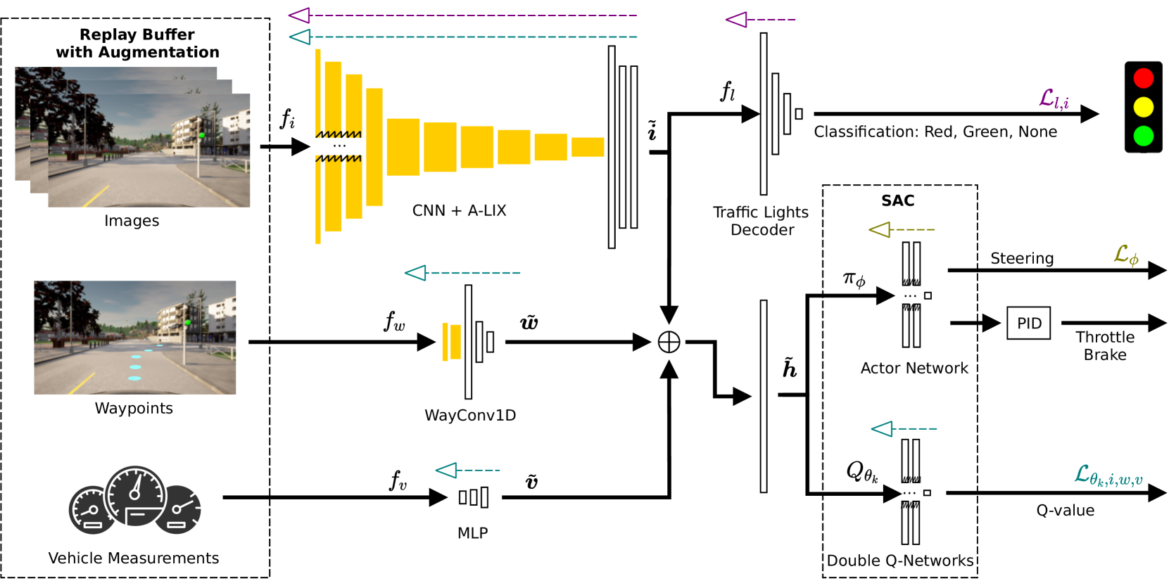
Figure 1: Architecture of RLAD. As input, the system receives $K$ consecutive central images, $N$ waypoints computed using a global planner, and measurements from the vehicle from the last $K$ steps. Each input is processed independently by a different encoder. The latent representations of each input are then concatenated, forming the input of the SAC algorithm ($\tilde{\boldsymbol{h}}=\begin{bmatrix}\tilde{\boldsymbol{i}}&\tilde{\boldsymbol{w}}&\tilde{\boldsymbol{v}}\end{bmatrix}$). The actor network of the SAC, along with a PID, is responsible for outputting the command controls, while the Q-networks are responsible for outputting the value function. To guide $\tilde{\boldsymbol{i}}$ to contain information about the traffic lights, we add an auxiliary branch to perform traffic light classification. All elements of the neural networks are represented at scale. The dashed arrows provide a visual representation of how each loss function affects the parameters of the system in the backpropagation stage.

III-A Learning Environment

The learning environment is defined as a Partially Observable Markov Decision Process (POMDP). The environment was built by using the CARLA driving simulator (version 0.9.10.1) [27].

State space

$\mathcal{S}$ is defined by CARLA, containing the ground truth about the world. The agent has no access to the state of the environment.

Observation space

At each step the state $s_{t}\in\mathcal{S}$ generates the corresponding observation $o_{t}\in\mathcal{O}$, which is conveyed to the agent. An observation is a stack of $K=3$ sets of tensors from the last $K$ timesteps. Specifically, $o_{t}=\{(\boldsymbol{I},\boldsymbol{W},\boldsymbol{V})_{k}\}_{k=0}^{2}$, where: $\boldsymbol{I}$ is a 3$\times$256$\times$256 image, $\boldsymbol{W}$ corresponds to the 2D coordinates related to the vehicle, for the next $N=10$ waypoints provided by the global planner from CARLA, and $\boldsymbol{V}$ corresponds to a two-dimensional vector containing the current speed and steering of the vehicle.

Action Space

$\mathcal{A}$ is composed of three continuous actions: throttle, which ranges from 0 to 1; brake, which ranges from 0 to 1; and steering, which ranges from -1 to 1.

Reward function

We used the reward function defined in [28] because it has been shown to accurately guide the AD training.

Training

We used CARLA at 10 FPS. Similarly to [28], at the beginning of the episode, the start and target locations are randomly generated and the desired route is computed using the global planner. When the target location is reached, a new random target location is computed. The episode is terminated if one of the following conditions is met: collision, running a red traffic light, blocked, or if a predefined timeout is reached.

III-B Agent Architecture

The architecture of RLAD is depicted in Figure 1. In general, our system has three main components: an encoder (Section III-B1), an RL algorithm (Section III-B2), and an auxiliary loss (Section III-B3). To simplify the longitudinal control and ensure smooth control, we reparameterize the throttle and brake commands using a target speed. As such, a PID controller is appended at the end of the actor network that produces the corresponding throttle and brake commands that match the predicted target speed.

III-B1 Encoder

The encoder is responsible for transforming the data from the sensors ($o_{t}$) into a low-dimension feature vector ($\tilde{\boldsymbol{h}}_{t}$) to be processed by the RL algorithm.

Image Encoder

As demonstrated in [11], the size of the image encoder is a critical element in an RLfP method. Due to the weak signal of the RL loss, encoders commonly used in AD methods, such as ResNet50 [29] ($\sim$ 25M parameters) or Inception V3 [30] ($\sim$ 27M parameters), are impracticable. On the other side, small encoders, designed for scenarios of smaller complexity, such as IMPALA [31] ($\sim$ 0.22M parameters), cannot produce an adequate representation of the environment, which limits the performance of the driving agent. For urban AD, our findings suggest that the optimal configuration entails a trade-off between larger networks that are unsuitable for training with RL and smaller networks that cannot accurately perceive the environment. The architecture of the proposed image encoder is shown in Table I, containing around 1M parameters. Similarly to DrQ and DrQ-V2, we leverage simple image augmentations to regularize the value function [11, 25]. First, we apply padding to each side of the 256$\times$256 image by repeating the 8 boundary pixels and then selecting a random crop of 256$\times$256. As in [25], we found it useful to apply bilinear interpolation on the cropped images. In addition to the image augmentations, we also found that appending an A-LIX layer [12] at the end of each convolution layer improves the performance of the agent, possibly by preventing a phenomenon called catastrophic self-overfitting (spatially inconsistent feature maps that lead to discontinuous gradients in the backpropagation). A-LIX is applied on the features produced by the convolution layers $a\in\mathbb{R}^{C\times H\times W}$, by randomly mixing each component $a_{cij}$ with its neighbors belonging to the same feature map. Consequently, the output of A-LIX is of the same dimensionality as the input, but with the difference that the computation graph minimally disrupts the information of each feature $a_{cij}$, while smoothing discontinuous component of the gradients signal during backpropagation [12]. Hence, this technique works by enforcing the image encoder to produce feature maps that are spatially consistent and thus minimizing the effect of the catastrophic self-overfitting phenomenon. This process can be succinctly summarized as $\tilde{\boldsymbol{i}}_{t}=f_{i}(\mathrm{aug}(\left[\{\boldsymbol{I}_{t-k}\}_{k=0}^{2}\right]))$ , where $f_{i}$ is the image encoder, $\mathrm{aug}$ corresponds to the data augmentation applied, and $\tilde{\boldsymbol{i}}_{t}$ corresponds to the latent representation of the stack of three consecutive images $\left(\left[\{\boldsymbol{I}_{t-k}\}_{k=0}^{2}\right]\right)$.

TABLE I: Architecture of the proposed image encoder. After each convolution layer, we applied the ReLU function [32] and the A-LIX regularizer layer [12].

type	kernel/stride	input size
$\mathrm{conv}$	3$\times$3/2	9$\times$256$\times$256
$\mathrm{conv}$	3$\times$3/2	32$\times$127$\times$127
$\mathrm{conv}$	3$\times$3/2	32$\times$63$\times$63
$\mathrm{conv}$	3$\times$3/2	32$\times$31$\times$31
$\mathrm{conv}$	3$\times$3/1	64$\times$15$\times$15
$\mathrm{conv}$	3$\times$3/1	64$\times$13$\times$13
$\mathrm{conv}$	3$\times$3/1	64$\times$11$\times$11
$\mathrm{conv}$	3$\times$3/1	64$\times$9$\times$9
$\mathrm{conv}$	3$\times$3/1	64$\times$7$\times$7
$\mathrm{flatten}$	-	64$\times$5$\times$5
$\mathrm{linear}$	-	1600
$\mathrm{layernorm}$	-	256
$\mathrm{tanh}$	-	256

Waypoint Encoder

Usually, the waypoint encoder consists of using the mean orientation between the current pose of the agent and the next $N$ waypoints [9] or flattening the waypoints’ 2D coordinates into a vector and then applying an MLP [33]. In our point of view, both approaches have serious limitations. The former approach clearly oversimplifies the problem by encoding all waypoint coordinates into a single value. This method only works for small values of $N$, because as $N$ increases, the waypoints become more scattered, and thus the mean orientation ceases to be a reliable indicator. Although the latter approach works for all values of $N$, by flattening the 2D waypoint coordinates into a vector, the 2D geometrical information is not being used. To overcome both limitations, we propose WayConv1D, a waypoint encoder that leverages the 2D geometrical structure of the input by applying 1D convolutions with a 2$\times$2 kernel over the 2D coordinates of the next $N$ waypoints. The output of the 1D convolution is then flattened and processed by an MLP. This process can be summarized as $\tilde{\boldsymbol{w}}_{t}=f_{w}(\boldsymbol{W}_{t})$, where $f_{w}$ corresponds to the WayConv1D, and $\tilde{\boldsymbol{w}}_{t}$ corresponds to the latent representation of the waypoints for the current step ($\boldsymbol{W}_{t}$). We found that with WayConv1D, the agent learns more efficiently to follow the trajectory without oscillating near the center of the lane. This is a common issue encountered when utilizing RL in the urban AD domain, as documented in previous studies [28, 6].

Vehicle Measurements Encoder

Similarly to [33], we apply an MLP to the vehicle measurements: $\tilde{\boldsymbol{v}}_{t}=f_{v}(\left[\{\boldsymbol{V}_{t-k}\}_{k=0}^{2}\right])$, where $f_{v}$ is the MLP, and $\tilde{\boldsymbol{v}}_{t}$ corresponds to the latent representation of the concatenation of the vehicle measurements across three steps $\left(\left[\{\boldsymbol{V}_{t-k}\}_{k=0}^{2}\right]\right)$.

III-B2 RL Algorithm

As the RL algorithm, we use the SAC [23], which is a model-free off-policy actor-critic algorithm that learns two Q-functions $Q_{\theta_{1}}$, $Q_{\theta_{2}}$, a stochastic policy $\pi_{\phi}$, and a temperature $\alpha$ to find an optimal policy by optimizing a $\gamma$-discounted maximum-entropy objective [34, 11]. The actor policy $\pi_{\phi}(a_{t}\mid\tilde{\boldsymbol{h}}_{t})$ is a parametric $\mathrm{tanh}$-Gaussian that given $\tilde{\boldsymbol{h}}_{t}=\begin{bmatrix}\tilde{\boldsymbol{i}}_{t}&\tilde{\boldsymbol{w}}_{t}&\tilde{\boldsymbol{v}}_{t}\end{bmatrix}$, samples $a_{t}=\mathrm{tanh}\left(\mu_{\phi}(\tilde{\boldsymbol{h}}_{t})+\sigma_{\theta}(\tilde{\boldsymbol{h}}_{t})\epsilon\right)$, where $\epsilon\sim\mathcal{N}(0,1)$, and $\mu_{\phi}$ and $\sigma_{\phi}$ are the parametric mean and standard deviation. The double Q-networks are learned by optimizing a single step of the soft Bellman residual:

$$\begin{split}\mathcal{L}_{\theta_{k},i,w,v}=\mathbb{E}_{\begin{subarray}{c}o_{t},a_{t},o_{t+1}\sim\mathcal{D}\\ a_{t+1}^{\prime}\sim\pi_{\phi}(\cdot\mid\tilde{\boldsymbol{h}}_{t+1})\end{subarray}}\left[\left(Q_{\theta_{k}}\left(\tilde{\boldsymbol{h}}_{t},a_{t}\right)-y\right)^{2}\right],\\ \forall k\in\{1,2\},\end{split}$$ (1)

with the TD target $y$ defined as:

$$\begin{split}y=r_{t}+\gamma\biggl{(}\smash{\displaystyle\min_{k=1,2}}Q_{\bar{\theta}_{k}}\left(\tilde{\boldsymbol{h}}_{t+1},a_{t+1}^{\prime}\right)-\\ \alpha\log\pi_{\phi}\left(a_{t+1}^{\prime}\mid\tilde{\boldsymbol{h}}_{t+1}\right)\biggr{)},\end{split}$$ (2)

where $\mathcal{D}$ represents the replay buffer, $r_{t}$ is the reward received, $\gamma$ is the discount factor, and $Q_{\bar{\theta}_{1}}$ and $Q_{\bar{\theta}_{2}}$ denote the Exponential Moving Average (EMA)of the parameters of $Q_{\theta_{1}}$ and $Q_{\theta_{2}}$, respectively. Similarly to DrQ-V2, we found it useful to use a single encoder, rather than a main encoder and an EMA of the main encoder. The policy is updated to maximize the expected future return plus the expected future entropy:

$$\begin{split}\mathcal{L}_{\phi}=-\mathbb{E}_{\begin{subarray}{c}{o_{t}\sim\mathcal{D}}\\ a_{t}\sim\pi_{\phi}(\cdot\mid\tilde{\boldsymbol{h}}_{t})\end{subarray}}\biggl{[}\smash{\displaystyle\min_{k=1,2}}Q_{\theta_{k}}\left(\tilde{\boldsymbol{h}}_{t},a_{t}\right)-\\ \alpha\log\pi\left(a_{t}\mid\tilde{\boldsymbol{h}}_{t}\right)\biggr{]}.\end{split}$$ (3)

Finally, the temperature $\alpha$ is learned using the loss proposed by Haarnoja et al., [35].

As noted in Equation 1 and 3, not all losses are propagated to the encoders. Following [18], we block the actor’s gradients from propagating to the encoder. In contrast with DrQ-V2, we found that using a learning rate of $10^{-3}$, instead of $10^{-4}$, results in a faster and more stable training. One intuition to explain this improvement is related to the observation space. DrQ-V2 was evaluated in tasks where the observation space is likely task-relevant, whereas in AD the observation space contains task-irrelevant information, such as clouds and buildings. Thus, with a larger learning rate, the encoder will learn faster to distinguish the task-relevant objects from the non-relevant, which prevents the agent from exploring using unreliable representations of the environment.

III-B3 Auxiliary Loss

Based on initial experiments, we observed that the agent struggled to associate the color of the traffic light with the negative reward incurred when passing through a red light. This is understandable, particularly when we take into account that the traffic light color occupies only a small fraction of the entire image. To address this issue, we implemented an auxiliary loss that strengthens the significance of traffic light information in the latent representation of the image ($\tilde{\boldsymbol{i}}$). As such, we added a traffic light decoder ($f_{l}$) to the end of the image encoder and perform traffic light classification using three classes ($C=3$): None, Red, and Green. None signifies that there is no traffic light within the vicinity of the agent, Red indicates the presence of a red or yellow traffic light near the agent, and finally, Green denotes a green traffic light near the agent. Every time we sample a batch of transitions from the replay buffer, we perform traffic light classification using the cross-entropy loss:

$$\mathcal{L}_{l,i}=-\sum_{b=1}^{B}\sum_{c=1}^{C}\log\left(\frac{e^{\left(x_{b,c}\right)}}{\sum_{i=1}^{C}e^{\left(x_{b,i}\right)}}\right)y_{b,c},$$ (4)

where $B$ is the batch size, $x$ corresponds to the logits outputted by $f_{l}$, and $y$ corresponds to the ground truth class. In the backpropagation stage, this loss updates both the parameters of the traffic light decoder and the parameters of the image encoder.

IV Experiments

In this section, we compare RLAD with the state-of-the-art RLfP methods, applied to the domain of urban AD. First, we define the setup of the experiments, and then compare RLAD with the state-of-the-art methods both in terms of expected return and using specific metrics related to urban AD. Finally, we present an ablation study that guided the development of RLAD.

IV-A Setup

Benchmark

The methods are evaluated on the NoCrash benchmark [36]. This benchmark considers generalization from Town 1, a town composed of one-lane roads and T-junctions with traffic lights, to Town 2, which is a scaled-down version of Town 1 with different textures. The training is performed using four training weather types, and the testing uses two different weather types. This benchmark has three levels of traffic density (empty, regular, and dense) according to the number of vehicles and pedestrians. The results are reported in terms of success rate, which is the percentage of routes completed without collision. Additionally, we also report information related to the percentage of route completion, red light infractions, collisions with vehicles, pedestrians, and layout, and blockages per kilometer.

Training Details

All algorithms are trained on the same hardware: a single NVIDIA RTX 2080 Ti. The algorithms are trained for $10^{6}$ environment steps and are evaluated every $20\,000$ environment steps. Each evaluation query averages episode returns over 10 episodes. The Deep Learning library used was PyTorch [37]. The list with the main hyperparameters used is present in Table II.

TABLE II: List of the hyperparameters used by RLAD.

Parameter	Value
Replay Buffer capacity	100000
Batch size	256
Action repeat	2
Discount factor $\gamma$	0.99
Optimizer	Adam [38]
Learning rate	$10^{-3}$
Critic target update frequency	1
Critic Q-function soft update rate	0.01
Critic update frequency	1
Actor update frequency	1
Auxiliary loss update frequency	1
$\mathrm{dim}(\tilde{\boldsymbol{i}})$	256
$\mathrm{dim}(\tilde{\boldsymbol{w}})$	32
$\mathrm{dim}(\tilde{\boldsymbol{v}})$	16
SAC networks size	1024
Actor log stddev bounds	[-10,2]
Init temperature	0.1

Baselines

Given that we are the first to propose an RLfP method applied in urban AD, we compare our method with the state-of-the-art RLfP methods: SAC+AE [18], CURL [24], DrQ [11], and DrQ-V2 [25]. The official implementation of these methods only uses images as input, so we added two additional encoders: a waypoint encoder similar to [33], and a vehicle measurement encoder similar to ours. These encoders were selected because they are the most commonly utilized in the end-to-end AD field. For a fair comparison, we also reparameterize the throttle and brake commands using a PID controller.

IV-B Comparison with Baselines

Figure 2 depicts the average return for each method during the NoCrash benchmark’s training process. It is evident that RLAD significantly outperforms all state-of-the-art methods. By the end of the training, RLAD manages to attain an average return that is roughly three times greater than all other methods.

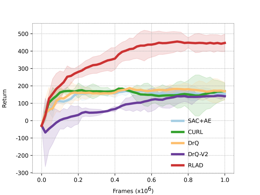
Figure 2: Comparison of RLAD with state-of-the-art RLfP methods in terms of average return per episode on the NoCrash benchmark. The solid lines represent the mean performance over 3 seeds, and the shaded regions represent $90\text{\,}\mathrm{\char 37\relax}$ confidence intervals.

Table III shows the performance of the algorithms in terms of success rate for every task of the NoCrash benchmark under testing conditions. In the empty task, all algorithms perform reasonably well, with the exception of DrQ-V2. However, as the difficulty of the task increases, the difference between the performance of RLAD and the other methods becomes more evident. Although RLAD performs equally to DrQ in the empty task, it outperforms the second best method by $50\text{\,}\mathrm{\char 37\relax}$ in the regular task and by $220\text{\,}\mathrm{\char 37\relax}$ in the dense task.

TABLE III: Success rate ($\mathrm{\char 37\relax}$) on NoCrash benchmark for each task in testing conditions (Town 2 with new weather). The results for each method correspond to the best seed considering the average episode return (Figure 2). Best scores for each task highlighted in bold.

	Empty	Regular	Dense
SAC+AE	82	42	6
CURL	74	30	2
DrQ	94	42	10
DrQ-V2	10	8	0
RLAD	94	62	32

Table V provides a detailed analysis of the performance of the methods with respect to AD-related metrics, specifically through an infraction analysis conducted on the regular task of the NoCrash benchmark. With the exception of DrQ-V2, all state-of-the-art RLfP methods achieve a route completion over $90\text{\,}\mathrm{\char 37\relax}$, but achieve a success rate of less than $50\text{\,}\mathrm{\char 37\relax}$. This clearly shows that the state-of-the-art RLfP methods are very good at following the trajectory generated by the global planner, but struggle to deal with dynamic obstacles, as is the case of vehicles and pedestrians. In contrast, RLAD is capable of dealing with dynamic obstacles, achieving the best score for all metrics related to collisions. The scores related to the red light infractions clearly demonstrate that obeying the traffic lights is a challenging task for RLfP algorithms. RLAD with the auxiliary loss is able to perform $17\text{\,}\mathrm{\char 37\relax}$ better when compared with the second best, but still very poorly when compared with state-of-the-art methods that use IL [39, 40, 41]. This limitation arises from the impracticability of using large image encoders in RLfP, which makes it challenging to create representations of the environment that include small yet important features, such as the color of traffic lights. Among all methods, DrQ-V2 is the one that performs worse in virtually all metrics. Internal investigations showed that the primary reason for this performance was the RL algorithm used - DDPG. Using our training conditions, DDPG quickly converges to a suboptimal policy, where the agent tends to remain still in various situations. This problem can be easily identified in the column related to the blockages of DrQ-V2: 22.14 blockages per kilometer.

Although RLAD outperforms all RLfP methods in the urban AD domain, it is not yet competitive with state-of-the-art RL methods that decouple the training of encoder and the policy network [6, 16, 8]. However, in the field of continuous control tasks in the MuJoCo simulator [42], RLfP methods have already surpassed those that decouple the encoder from the policy network, which suggests that the same pattern may occur in the urban AD domain as well. Furthermore, the image encoder of state-of-the-art RL methods that decouple the encoder from the policy network contains around 25 times more parameters than the image encoder of RLAD [6, 16, 8], requiring more computation power and resources, which may compromise their application in real-time settings.

TABLE IV: Driving performance and infraction analysis on the NoCrash benchmark, using the regular task in testing conditions. The results for each method correspond to the best seed considering the average episode return (Figure 2). Best scores highlighted in bold.

	Success rate	Route completion	Collision pedestrian	Collision vehicle	Collision layout	Red light infraction	Agent blocked
	$\mathrm{\char 37\relax}$, $\uparrow$	$\mathrm{\char 37\relax}$,$\uparrow$	#/Km, $\downarrow$	#/Km, $\downarrow$	#/Km, $\downarrow$	#/Km $\downarrow$	#/Km, $\downarrow$
SAC+AE	42	98	0.60	1.71	0.99	6.16	0.23
CURL	30	99	0.97	1.91	1.68	6.81	0.20
DrQ	42	100	0.77	1.51	0.19	7.35	0.00
DrQ-V2	8	53	0.58	1.68	1.63	7.04	22.14
RLAD	62	94	0.41	0.71	0.16	5.10	0.84

TABLE V: Driving performance and infraction analysis on the NoCrash benchmark, using the regular task in testing conditions. The results for each method correspond to the best seed considering the average episode return (Figure 2). Best scores highlighted in bold.

IV-C Ablation Study

We performed three experiments: using the waypoint encoder of [33] instead of WayConv1D; removal of the auxiliary loss; and removal of the A-LIX layers. Figure 3 shows the influence of each of these components in terms of the average return per episode. The most impactful components are the auxiliary loss and the A-LIX layers. Removing them results in a performance decrease of $33\text{\,}\mathrm{\char 37\relax}$. Replacing the WayConv1D by the waypoint encoder of [33] results in a performance decrease of $15\text{\,}\mathrm{\char 37\relax}$. Furthermore, this replacement also leads to more oscillations near the center lane, resulting in a less comfortable driving experience.

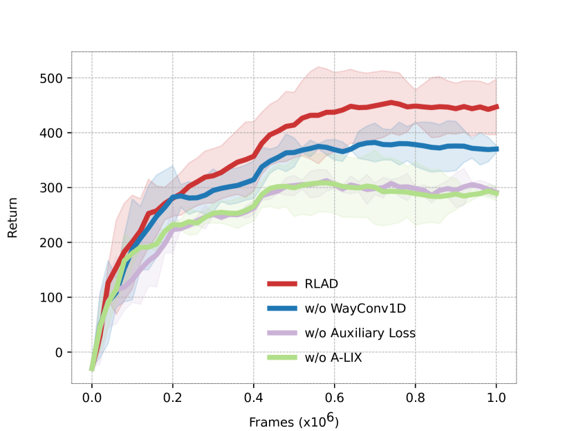
Figure 3: Ablation study that guided the development of RLAD. The solid lines represent the mean performance over 3 seeds, and the shaded regions represent $90\text{\,}\mathrm{\char 37\relax}$ confidence intervals.

V Conclusion

This paper introduced RLAD, the first algorithm that learns simultaneously the encoder and the driving policy network using Reinforcement Learning (RL)in the domain of vision-based urban Autonomous Driving (AD). Our method significantly outperforms all RLfP state-of-the-art methods in this domain. Although our method is not yet competitive with the state-of-the-art methods in end-to-end urban AD, we believe that RLAD can foster the interest in applying RLfP to the domain of urban AD. Methods that learn simultaneously the encoder and the policy network have demonstrated better performance in the continuous control tasks in the MuJoCo simulator, compared to those that decouple the encoder from the policy network. Based on this information, we have grounds to expect that a comparable pattern will emerge in the realm of urban AD, and we believe that RLAD constitutes the first step toward this end.

References

- [1] D. Fernandes, A. Silva, R. Névoa, C. Simões, D. Gonzalez, M. Guevara, P. Novais, J. Monteiro, and P. Melo-Pinto, “Point-cloud based 3D object detection and classification methods for self-driving applications: A survey and taxonomy,” Information Fusion, vol. 68, pp. 161–191, 2021. [Online]. Available: https://www.sciencedirect.com/science/article/pii/S1566253520304097
- [2] D. Coelho and M. Oliveira, “A review of end-to-end autonomous driving in urban environments,” IEEE Access, vol. 10, pp. 75 296–75 311, 2022.
- [3] Y. Wu, S. Liao, X. Liu, Z. Li, and R. Lu, “Deep Reinforcement Learning on Autonomous Driving Policy With Auxiliary Critic Network,” IEEE Transactions on Neural Networks and Learning Systems, pp. 1–11, 2021.
- [4] K. Chitta, A. Prakash, and A. Geiger, “Neat: Neural attention fields for end-to-end autonomous driving,” 2021 IEEE/CVF International Conference on Computer Vision (ICCV), pp. 15 773–15 783, 2021.
- [5] Z. Huang, S. Sun, J. Zhao, and L. Mao, “Multi-modal policy fusion for end-to-end autonomous driving,” Information Fusion, vol. 98, p. 101834, 2023. [Online]. Available: https://www.sciencedirect.com/science/article/pii/S1566253523001501
- [6] M. Toromanoff, É. Wirbel, and F. Moutarde, “End-to-end model-free reinforcement learning for urban driving using implicit affordances,” 2020 IEEE/CVF Conference on Computer Vision and Pattern Recognition (CVPR), pp. 7151–7160, 2019.
- [7] M. Oliveira, V. Santos, and A. D. Sappa, “Multimodal inverse perspective mapping,” Information Fusion, vol. 24, pp. 108–121, 2015. [Online]. Available: https://www.sciencedirect.com/science/article/pii/S1566253514001031
- [8] M. Ahmed, A. Abobakr, C. P. Lim, and S. Nahavandi, “Policy-Based Reinforcement Learning for Training Autonomous Driving Agents in Urban Areas With Affordance Learning,” IEEE Transactions on Intelligent Transportation Systems, vol. 23, no. 8, pp. 12 562–12 571, 2022.
- [9] T. Agarwal, H. Arora, and J. Schneider, “Learning Urban Driving Policies using Deep Reinforcement Learning,” IEEE Conference on Intelligent Transportation Systems, Proceedings, ITSC, vol. 2021-September, pp. 607–614, 2021.
- [10] R. Chekroun, M. Toromanoff, S. Hornauer, and F. Moutarde, “Gri: General reinforced imitation and its application to vision-based autonomous driving,” ArXiv, vol. abs/2111.08575, 2021.
- [11] I. Kostrikov, D. Yarats, and R. Fergus, “Image augmentation is all you need: Regularizing deep reinforcement learning from pixels,” ArXiv, vol. abs/2004.13649, 2020.
- [12] E. Cetin, P. J. Ball, S. Roberts, and O. Çeliktutan, “Stabilizing off-policy deep reinforcement learning from pixels,” in International Conference on Machine Learning, 2022.
- [13] V. Mnih, K. Kavukcuoglu, D. Silver, A. Graves, I. Antonoglou, D. Wierstra, and M. A. Riedmiller, “Playing atari with deep reinforcement learning,” ArXiv, vol. abs/1312.5602, 2013.
- [14] E. Todorov, T. Erez, and Y. Tassa, “Mujoco: A physics engine for model-based control,” in 2012 IEEE/RSJ International Conference on Intelligent Robots and Systems, 2012, pp. 5026–5033.
- [15] A. Zhang, R. McAllister, R. Calandra, Y. Gal, and S. Levine, “Learning invariant representations for reinforcement learning without reconstruction,” ArXiv, vol. abs/2006.10742, 2020.
- [16] Y. Zhao, K. Wu, Z. Xu, Z. Che, Q. Lu, J. Tang, and C. H. Liu, “Cadre: A cascade deep reinforcement learning framework for vision-based autonomous urban driving,” in AAAI Conference on Artificial Intelligence, 2022.
- [17] C. Huang, R. Zhang, M. Ouyang, P. Wei, J. Lin, J. Su, and L. Lin, “Deductive Reinforcement Learning for Visual Autonomous Urban Driving Navigation,” IEEE Transactions on Neural Networks and Learning Systems, vol. 32, no. 12, pp. 5379–5391, 2021.
- [18] D. Yarats, A. Zhang, I. Kostrikov, B. Amos, J. Pineau, and R. Fergus, “Improving sample efficiency in model-free reinforcement learning from images,” in AAAI Conference on Artificial Intelligence, 2019.
- [19] M. Hessel, J. Modayil, H. V. Hasselt, T. Schaul, G. Ostrovski, W. Dabney, D. Horgan, B. Piot, M. G. Azar, and D. Silver, “Rainbow: Combining improvements in deep reinforcement learning,” ArXiv, vol. abs/1710.02298, 2017.
- [20] J. Schulman, F. Wolski, P. Dhariwal, A. Radford, and O. Klimov, “Proximal policy optimization algorithms,” ArXiv, vol. abs/1707.06347, 2017.
- [21] E. Shelhamer, P. Mahmoudieh, M. Argus, and T. Darrell, “Loss is its own reward: Self-supervision for reinforcement learning,” ArXiv, vol. abs/1612.07307, 2016.
- [22] V. Mnih, A. P. Badia, M. Mirza, A. Graves, T. P. Lillicrap, T. Harley, D. Silver, and K. Kavukcuoglu, “Asynchronous methods for deep reinforcement learning,” ArXiv, vol. abs/1602.01783, 2016.
- [23] T. Haarnoja, A. Zhou, P. Abbeel, and S. Levine, “Soft actor-critic: Off-policy maximum entropy deep reinforcement learning with a stochastic actor,” in International Conference on Machine Learning, 2018.
- [24] A. Srinivas, M. Laskin, and P. Abbeel, “Curl: Contrastive unsupervised representations for reinforcement learning,” in International Conference on Machine Learning, 2020.
- [25] D. Yarats, R. Fergus, A. Lazaric, and L. Pinto, “Mastering visual continuous control: Improved data-augmented reinforcement learning,” ArXiv, vol. abs/2107.09645, 2021.
- [26] T. P. Lillicrap, J. J. Hunt, A. Pritzel, N. M. O. Heess, T. Erez, Y. Tassa, D. Silver, and D. Wierstra, “Continuous control with deep reinforcement learning,” CoRR, vol. abs/1509.02971, 2015.
- [27] A. Dosovitskiy, G. Ros, F. Codevilla, A. M. López, and V. Koltun, “Carla: An open urban driving simulator,” ArXiv, vol. abs/1711.03938, 2017.
- [28] Z. Zhang, A. Liniger, D. Dai, F. Yu, and L. V. Gool, “End-to-end urban driving by imitating a reinforcement learning coach,” 2021 IEEE/CVF International Conference on Computer Vision (ICCV), pp. 15 202–15 212, 2021.
- [29] K. He, X. Zhang, S. Ren, and J. Sun, “Deep residual learning for image recognition,” 2016 IEEE Conference on Computer Vision and Pattern Recognition (CVPR), pp. 770–778, 2015.
- [30] C. Szegedy, V. Vanhoucke, S. Ioffe, J. Shlens, and Z. Wojna, “Rethinking the inception architecture for computer vision,” 2016 IEEE Conference on Computer Vision and Pattern Recognition (CVPR), pp. 2818–2826, 2015.
- [31] L. Espeholt, H. Soyer, R. Munos, K. Simonyan, V. Mnih, T. Ward, Y. Doron, V. Firoiu, T. Harley, I. Dunning, S. Legg, and K. Kavukcuoglu, “Impala: Scalable distributed deep-rl with importance weighted actor-learner architectures,” ArXiv, vol. abs/1802.01561, 2018.
- [32] A. F. Agarap, “Deep learning using rectified linear units (relu),” ArXiv, vol. abs/1803.08375, 2018.
- [33] P. Cai, S. Wang, Y. Sun, and M. Liu, “Probabilistic end-to-end vehicle navigation in complex dynamic environments with multimodal sensor fusion,” IEEE Robotics and Automation Letters, vol. 5, pp. 4218–4224, 2020.
- [34] B. D. Ziebart, A. L. Maas, J. A. Bagnell, and A. K. Dey, “Maximum entropy inverse reinforcement learning,” in AAAI Conference on Artificial Intelligence, 2008.
- [35] T. Haarnoja, A. Zhou, K. Hartikainen, G. Tucker, S. Ha, J. Tan, V. Kumar, H. Zhu, A. Gupta, P. Abbeel, and S. Levine, “Soft actor-critic algorithms and applications,” ArXiv, vol. abs/1812.05905, 2018.
- [36] F. Codevilla, E. Santana, A. M. López, and A. Gaidon, “Exploring the limitations of behavior cloning for autonomous driving,” 2019 IEEE/CVF International Conference on Computer Vision (ICCV), pp. 9328–9337, 2019.
- [37] A. Paszke, S. Gross, F. Massa, A. Lerer, J. Bradbury, G. Chanan, T. Killeen, Z. Lin, N. Gimelshein, L. Antiga, A. Desmaison, A. Köpf, E. Yang, Z. DeVito, M. Raison, A. Tejani, S. Chilamkurthy, B. Steiner, L. Fang, J. Bai, and S. Chintala, “Pytorch: An imperative style, high-performance deep learning library,” in Neural Information Processing Systems, 2019.
- [38] D. P. Kingma and J. Ba, “Adam: A method for stochastic optimization,” CoRR, vol. abs/1412.6980, 2014.
- [39] K. Chitta, A. Prakash, B. Jaeger, Z. Yu, K. Renz, and A. Geiger, “Transfuser: Imitation with transformer-based sensor fusion for autonomous driving,” IEEE transactions on pattern analysis and machine intelligence, vol. PP, 2022.
- [40] H.-C. Shao, L. Wang, R. Chen, H. Li, and Y. T. Liu, “Safety-enhanced autonomous driving using interpretable sensor fusion transformer,” ArXiv, vol. abs/2207.14024, 2022.
- [41] D. Chen and P. Krähenbühl, “Learning from all vehicles,” 2022 IEEE/CVF Conference on Computer Vision and Pattern Recognition (CVPR), pp. 17 201–17 210, 2022.
- [42] Y. Tassa, Y. Doron, A. Muldal, T. Erez, Y. Li, D. de Las Casas, D. Budden, A. Abdolmaleki, J. Merel, A. Lefrancq, T. P. Lillicrap, and M. A. Riedmiller, “Deepmind control suite,” ArXiv, vol. abs/1801.00690, 2018.