Escaping mediocrity: how two-layer networks
learn hard single-index models with SGD

Abstract

This study explores the sample complexity for two-layer neural networks to learn a single-index target function under Stochastic Gradient Descent (SGD), focusing on the challenging regime where many flat directions are present at initialization. It is well-established that in this scenario $n=O(d\log{d})$ samples are typically needed. However, we provide precise results concerning the pre-factors in high-dimensional contexts and for varying widths. Notably, our findings suggest that overparameterization can only enhance convergence by a constant factor within this problem class. These insights are grounded in the reduction of SGD dynamics to a stochastic process in lower dimensions, where escaping mediocrity equates to calculating an exit time. Yet, we demonstrate that a deterministic approximation of this process adequately represents the escape time, implying that the role of stochasticity may be minimal in this scenario.

1 Introduction

In this manuscript we are interested in the supervised task of learning the following target function:

$$y=\sigma_{\star}\left(w_{\star}^{\top}x\right)+\sqrt{\Delta}z, x\sim\mathcal{N}(0,\nicefrac{{1}}{{d}}I_{d}),\qquad z\sim\mathcal{N}(0,1).$$ (1)

This target belongs to a general class of models known as single-index or generalised linear models, where the labels depend on the covariates $x\in\mathbb{R}^{d}$ only through its projection on a fixed direction $w_{\star}\in\mathbb{R}^{d}$, followed by a non-linear real-valued function $\sigma_{\star}\mathrel{\mathop{\mathchar 58\relax}}\mathbb{R}\to\mathbb{R}$. Despite its apparent simplicity, the study of single-index models with Gaussian i.i.d. covariates has been at the core of the recent theoretical progress in machine learning [1, 2, 3, 4, 5]. Note that if $\sigma(x)=x$, learning could be achieved efficiently by linear methods such as ridge regression or PCA. The presence of a non-linearity $\sigma_{\star}$ makes it perhaps the simplest target for which a non-linear hypothesis class is required. Moreover, the choice of isotropic covariates $x\sim\mathcal{N}(0,\nicefrac{{1}}{{d}}I_{d})$ means that all structure in the target is in learning a representation of $\sigma$ and a particular direction $w_{\star}$. The popularity of this model is that different separation results can be shown in the high-dimensional limit where $d\gg 1$:

• In the well-specified setting where we fit an isotropic single-index model with the same hypothesis class (i.e. $f_{\theta}(x)=\sigma_{\star}(w^{\top}x)$), it has been shown that the sample complexity of one-pass SGD is determined by the first non-zero Hermite coefficient of the target $\sigma_{\star}$, also known as the information exponent [2]. Problems with non-zero first Hermite have information exponent $k=1$, and $w_{\star}$ can be learned at linear sample complexity $n=O(d)$. Instead, problems with zero first and non-zero second Hermite coefficient have information exponent $k=2$, requiring instead $n=O(d\log{d})$ samples [1, 2]. Note that this is a factor $\log{d}$ higher than the Bayes-optimal sample complexity of $n=O(d)$ [6, 7], hence defining a class of hard problems for SGD.

• For fully-connected two-layer neural networks $f_{\theta}(x)=a^{\top}\sigma(Wx)$, several results are known under different assumptions. For fixed first layer weights $W\in\mathbb{R}^{p\times d}$ (a.k.a. random features model) and large enough width $p$, learning the $k$-th order Hermite coefficient $\sigma_{\star}$ requires $n=O(d^{k})$ samples [8], implying a sample complexity of $n=O(d^{2})$ for a quadratic problem, e.g. $\sigma_{\star}(x)=x^{2}$. Recently, it was shown that wide networks ($p\to\infty$) can achieve the well-specified sample complexity of $n=O(d)$ under one-pass SGD, provided that all Hermite coefficients of both $\sigma_{\star},\sigma$ are non-zero [5]. In particular, this assumption cover only problems with information exponent $k=1$, excluding hard cases such as quadratic problems. Finally, for $\sigma(x)=\sigma_{\star}(x)=x^{2}$, [9] has shown that for $p$ large enough, full-batch gradient flow achieves sample complexity $n=2d$, although at a running time of $t=O(\log{d})$.

With the exception of [5], the works mentioned above cover the scaling of the sample complexity in the high-dimensional limit. Our goal is, instead, to derive sharp results for the sample complexity of learning (1) with a fully-connected two-layer neural network in the challenging case where $\sigma_{\star}$ has a vanishing first Hermite coefficient. As discussed above, this case violates the “standard learning scenario” of [5], and can be seen as a proxy for hard learning problems for descent-based algorithms. For concreteness, in the following we focus on the purely quadratic case:

$$y=\left(w_{\star}^{\top}x\right)^{2}+\sqrt{\Delta}z, w_{\star}\in\mathbb{S}^{d-1}(\sqrt{d})$$ (2)

Learning the target (2) consists of learning the non-linearity $\sigma_{\star}(x)=x^{2}$ and the direction $w_{\star}$. In this work, we focus our attention in the second part, considering the following architecture with squared-activation:

$$f_{\Theta}(x)=\frac{1}{p}\sum\limits_{i=1}^{p}a_{i}(w_{i}^{\top}x)^{2}.$$ (3)

where $\Theta=(a,W)$ is the set of trainable weights, which are trained with one-pass stochastic gradient descent (SGD):

$$\Theta^{\nu+1}=\Theta^{\nu}-\gamma\nabla_{\Theta}\ell(y^{\nu},f_{\Theta^{\nu}}(x^{\nu}))$$ (4)

with square loss $\ell(y,x)=\nicefrac{{1}}{{2}}(y-x)^{2}$ and initial condition $\Theta^{0}=(a^{0},W^{0})$. Note that at each step $\nu$, the gradient is evaluated at a fresh pair of data $(x^{\nu},y^{\nu})\in\mathbb{R}^{d+1}$ drawn from the model (2). In particular, this implies that after $\nu\in[n]$ steps, the algorithm has seen $n$ data points.

Learning in this problem is hard, and can be compared to finding a needle in a haystack. Indeed, with the exception of one direction that points towards $\pm w_{\star}$, the population risk at (random) initialization is mostly flat. This slows down the dynamics, which takes a long time to establish a significant correlation with the signal - a scenario we refer to as escaping mediocrity.

At first, the particular case of purely quadratic activation might appear too specific. Indeed, as we will see later the population risk for this task has a a global maximum at initialization and a degenerated set of global minima. The choice of more general $\sigma_{\star}$ and $\sigma$ with zero first Hermite but not necessarily zero higher-order coefficients might give rise to other critical points such as saddle-points, giving rise to a more complex SGD dynamics. However, since the focus of this work is on escaping mediocrity, our conclusions will hold, up to constants, to more general activations with zero first Hermite.

Summary of results —

Our main contributions in this manuscript are:

• We derive a deterministic set of ODEs providing an exact and analytically tractable description of the one-pass SGD dynamics in the high-dimensional limit $d\to\infty$, and characterize the leading order stochastic corrections to this limit.

• We provide an analytical formula for the number of samples required for one-pass SGD to learn the phase retrieval target in high-dimensions at arbitrary network width. We show that overparametrization can only improve convergence by a constant factor for phase retrieval.

• Finally, we compute the leading order stochastic corrections to the exit time, and show that stochasticity does not help escaping the flat directions at initialization. This suggests that the deterministic descriptions is enough to fully capture the phenomenology of the dynamics in this problem.

All the codes used for numerical experiments are provided in this GitHub repository.

Further related work —

The investigation of a deterministic high-dimensional limit of one-pass SGD for two-layer neural networks draws back to the seminal works of [10, 11, 12], and was followed by a stream of works that span decades of research [13, 14, 15, 16, 17, 18, 19, 20]. More recently, the stochastic corrections around fixed points of the dynamics have been investigated by [21]. In a complementary research line, [22, 23, 24, 25, 26]) have shown that an alternative deterministic description of SGD can be obtained in the infinite width-limit, a.k.a. mean-field regime. High-dimensional reductions of the mean-field equations have been studied by [27, 28, 29, 5]. Recently, [19, 20] has shown that these apparently different limits of one-pass SGD can be unified in a single description.

There has been a recent surge of interest in studying how increasing degrees of complexity in the target function are incrementally learned by SGD [27, 28, 30, 31, 5], with an emerging staircase picture where complexity is sequentially learned in different scenarios. This picture, however, is bound to classes of targets where SGD develops strong correlations with the target directions at initialization, a notion which was mathematically formalized by the so-called information exponent (IE) by [2]. Instead, targets for which the landscape at initialization is mostly flat (${\rm IE}\geq 2$) are hard for SGD at high-dimensions, translating to very slow dynamics. This is precisely the case for the phase retrieval problem (${\rm IE=2}$), a classic inverse problem arising in many scientific areas, from X-ray crystallography to astronomical imaging [32, 33]. Phase retrieval has been widely studied in the literature as a prototypical example of a hard inverse problem [34, 35, 36, 37, 6, 38, 7], providing a simple yet challenging example of a non-convex optimization problem which is hard for descent-based algorithms [39, 1, 40, 41, 42, 9, 43, 44].

2 High-dimensional limit of SGD

In this section we introduce our key theoretical tool, which consists in low-dimensional reduction of the projected SGD dynamics (4) in the high-dimensional limit $d\to\infty$ of interest.

Sufficient statistics —

The key observation is to notice that the population risk only depends on the hidden-layer weights $W\in\mathbb{R}^{p\times d}$ through the the second layer weights $a\in\mathbb{R}^{p}$ and the weights correlation matrices:

$$\begin{split}\Omega\coloneqq\begin{pmatrix}Q&m\\ {m^{\top}}&1\end{pmatrix}=\begin{pmatrix}\nicefrac{{1}}{{d}}\mathrm{W}{\mathrm{W}}^{\top}&\nicefrac{{1}}{{d}}\mathrm{W}{w_{\star}}\\ \nicefrac{{1}}{{d}}\left(\mathrm{W}{w_{\star}}\right)^{\top}&1\end{pmatrix}\in\mathbb{R}^{(p+1)\times(p+1)},\end{split}$$ (5)

The explicit expression of the population risk is:

$$\mathcal{R}(\Theta) =\mathbb{E}\left[\ell(y,f_{\Theta}(x))\right]=\frac{\Delta+3}{2}-\frac{1}{p}\sum\limits_{j=1}^{p}a_{j}\left(Q_{jj}+2m_{j}^{2}\right)+\frac{1}{2p^{2}}\sum\limits_{j,l=1}^{p}a_{j}a_{l}(Q_{jj}Q_{ll}+2Q_{jl}^{2})$$ (6)

Notice that the matrices $M,Q$ are precisely the second moments of the pre-activations $(\lambda_{\star},\lambda)=(w_{\star}^{\top}x,Wx)\in\mathbb{R}^{p+1}$. Therefore, to characterize the evolution of the risk throughout SGD, it is sufficient to track the evolution of the first layer weights $a_{i}$ and the correlation matrices $m,Q$, which consists of $p(p+1)$ parameters. As shown in Appendix A, starting from Eq. (4) we can derive a set of self-consistent stochastic processes describing the evolution of $(a,m,Q)$:

$$a_{j}^{\nu+1}-a_{j}^{\nu} =\frac{\gamma}{pd}\mathcal{E}^{\nu}\lambda_{j}^{2}$$ (7)

$$m_{j}^{\nu+1}-m_{j}^{\nu} =2\frac{\gamma}{pd}\mathcal{E}^{\nu}a_{j}\lambda_{j}\lambda_{\star}\eqqcolon\mathcal{M}_{j}(a,\lambda_{\star},\lambda)$$ (8)

$$Q_{jl}^{\nu+1}-Q^{\nu}_{jl} =2\frac{\gamma}{pd}\mathcal{E}^{\nu}\left(a_{j}+a_{l}\right)\lambda_{j}\lambda_{l}+4\frac{\gamma^{2}}{p^{2}d}{\mathcal{E}^{\nu}}^{2}||x^{\nu}||^{2}a_{j}a_{l}\lambda_{j}\lambda_{l}\eqqcolon\mathcal{Q}_{jl}(a,\lambda_{\star},\lambda)$$ (9)

where we have defined the displacement vector

$$\mathcal{E}^{\nu}\coloneqq\frac{1}{p}\sum_{j=1}^{p}a_{j}(\lambda_{j}^{\nu})^{2}-(\lambda^{\star\nu})^{2}+\sqrt{\Delta}z^{\nu},$$ (10)

and we used $\nicefrac{{\gamma}}{{d}}$ as the learning rate of the second layer, in order to have the same high-dimensional scaling.

High-dimensional limit —

As of now we have not made any assumptions on the dimension of the problem; the stochastic processes defined in (7) are exact, with the right-hand side depending implicitly on $(m,Q)$ through the moments of $(\lambda_{\star},\lambda)$. However, our goal is to study this process in the high-dimensional limit $d\to\infty$ where learning is hard and simulating (4) can be computationally demanding. Defining a step-size $\delta t=\nicefrac{{\gamma}}{{pd}}$ and a continuous extension of $(a^{\nu},m^{\nu},Q^{\nu})$ to continuous time $(a(\nu\delta t),m(\nu\delta t),Q(\nu\delta t))$ by linear interpolation, it can be shown that in the high-dimensional limit $d\to\infty$ the sufficient statistics $(a(t),m(t),Q(t))$ concentrate in their expectation $(\bar{a}(t),\bar{m}(t),\bar{Q}(t))$, which satisfies the following system of ordinary differential equations (ODEs):

$$\begin{split}\mathinner{\dfrac{\operatorname{d\!}{}\bar{a}_{j}}{\operatorname{d\!}{t}}}&=\mathbb{E}_{(\lambda,\lambda_{\star})\sim\mathcal{N}(0_{p+1},\Omega)}\left[\mathcal{E}\lambda_{j}^{2}\right]\\ \mathinner{\dfrac{\operatorname{d\!}{}\bar{m}_{j}}{\operatorname{d\!}{t}}}&=\mathbb{E}_{(\lambda,\lambda_{\star})\sim\mathcal{N}(0_{p+1},\Omega)}\left[\mathcal{M}_{j}(a,\lambda_{\star},\lambda)\right]\eqqcolon\Psi_{j}\left(\Omega\right)\\ \mathinner{\dfrac{\operatorname{d\!}{}\bar{Q}_{jl}}{\operatorname{d\!}{t}}}&=\mathbb{E}_{(\lambda,\lambda_{\star})\sim\mathcal{N}(0_{p+1},\Omega)}\left[\mathcal{Q}_{jl}(a,\lambda_{\star},\lambda)\right]\eqqcolon\Phi_{jl}\left(\Omega\right)\end{split}$$ (11)

with initial conditions given by $(\bar{a}(0),\bar{m}(0),\bar{Q}(0))=(a^{0},\nicefrac{{1}}{{d}}W^{0}w_{\star},\nicefrac{{1}}{{d}}W^{0}{W^{0}}^{\top})$. The explicit expression of these expected values can be found in Appendix A. As discussed in the related works, the high-dimensional limit of one-pass SGD for two-layer neural networks have been studied under different settings in the literature [12, 16, 15, 40, 19, 20, 21, 5]. However, to our best knowledge our work is the first to derive and study these equations for the squared activation in the high-dimensional limit.

Initialization and mediocrity —

In the noiseless case $\Delta=0$, it is easy to check that $a_{j}=1$ and $w_{j}=\pm w_{\star}$ ($m_{j}=\pm 1$ and $Q_{jl}=1$) is indeed a stationary point of (11) that corresponds to two degenerated global minima of the population risk (6). Adding a noise $\Delta>0$ only shift these values. Similarly, it is easy to check that $m_{i}=0$ and $Q_{ij}=0$ for $i\neq j$ are also stationary points. These correspond to taking $w_{j}\perp w_{l}\perp w_{\star}$ for all $j\neq l$ in (11), and is a global maximum of (6). This stationary point plays an important role in the dynamics. Indeed, in the absence of knowledge on the process that generated the data (2), it is customary to initialize the weights randomly:

$$w^{0}_{j}\sim\mathcal{N}(0,I_{d}), j=1,\cdots,p.$$ (12)

When $d\to\infty$, the weights are be orthogonal with high probability. In terms of the sufficient statistics:

$$Q_{jj}\sim\text{Dirac}(1),\qquad j\neq l\mathrel{\mathop{\mathchar 58\relax}}\;\sqrt{d}\,Q^{0}_{jl}\xrightarrow{d\to+\infty}\mathcal{N}(0,1)\quad\text{and}\quad\sqrt{d}\,m^{0}_{j}\xrightarrow{d\to+\infty}\mathcal{N}(0,1).$$ (13)

Therefore, since the variance of $(m^{0},Q^{0})$ decays as $\nicefrac{{1}}{{d}}$, the higher the dimension, the closer a random initialization is to a stationary point of the dynamics. Moreover, of all the $d$ directions, there exists $d-p-1$ directions orthogonal to $w_{\star}$ and $\{w^{0}_{j}\}_{j\in[p]}$ along which the population risk (6) remains constant. The proliferation of flat directions close to initialization severely slows down the SGD dynamics at high-dimensions, which typically requires $n=O(d\log{d})$ steps to develop a significant correlation with the signal in order to escape this region. This scenario, which we refer to as escaping mediocrity, is common to many hard learning problems [2]. In the following, we leverage the exact description (11) derived in this section to estimate precisely how much data is required for SGD to escape mediocrity in the prototypical phase retrieval problem (1).

Spherical constraint —

A phenomenon that is observed when starting from the initial conditions above is a change in the norms of the weights $w_{i}$ without effectively correlating with $w_{\star}$. In this phase, sometimes referred as norm learning, $m\approx Q_{jl}\approx 0$ for $j\neq l$, while $Q_{jj}$ changes considerably, resulting in a slightly decrease in the population risk towards a plateau that reflects mediocrity. Since the focus of this study is precisely on escaping mediocrity (i.e. developing non-zero correlation with the signal), in the following we will fix the norm of the weights $w^{\nu}_{i}\in\mathbb{S}^{d-1}(\sqrt{d})$ at initialization and throughout the dynamics $\nu\in[n]$. This assumption, which was also the focus of [2], amounts to imposing a spherical constraint at every step of SGD, also known as projected SGD:

$$w_{j}^{\nu+1}=\frac{w_{j}^{\nu}-\gamma\nabla_{w_{j}}\ell(y^{\nu},f_{\Theta^{\nu}}(x^{\nu}))}{\left\lVert w_{j}^{\nu}-\gamma\nabla_{w_{j}}\ell(y^{\nu},f_{\Theta^{\nu}}(x^{\nu}))\right\rVert}\sqrt{d}.$$ (14)

The high-dimensional limit of these equations lead to the following ODEs for the evolution of the sufficient statistics $(M,Q)$:

$$\mathinner{\dfrac{\operatorname{d\!}{}\bar{m}_{j}}{\operatorname{d\!}{t}}}=\Psi_{j}{(\Omega)}-\frac{\bar{m}_{j}}{2}\Phi_{jj}{(\Omega)}, \mathinner{\dfrac{\operatorname{d\!}{}\bar{Q}_{jl}}{\operatorname{d\!}{t}}}=\Phi_{jl}{(\Omega)}-\frac{\bar{Q}_{jl}}{2}\left(\Phi_{jj}{(\Omega)}+\Phi_{ll}{(\Omega)}\right).$$ (15)

Note that $Q_{jj}=1$ is consistently fixed.

3 Escaping mediocrity in the well-specified scenario

As a starting point, we consider the well-specified case of $p=1$. As we are going to see, this case captures almost all of the phenomenology of interest, and is helpful to build an intuition for how SGD escapes mediocrity. Moreover, despite its apparent simplicity, this case has been the subject of several works in the literature [39, 1, 41, 2]. In particular, [41] established a convergence rate $t=O(\log{d})$ for randomly initialized gradient descent on the population risk. In our setting (4), this corresponds to the $\gamma\to 0^{+}$ limit, and translates to a sample complexity of $n=O(d\log{d})$. [1] provided a refined analysis that accounts for the stochasticity in one-pass SGD, reaching a similar $n=O(d\log{d})$ rate for escaping mediocrity, in agreement with the general information exponent characterization of [2].

In this section, we show that in the high-dimensional limit, the sample complexity constant for one-pass SGD can be well estimated from the deterministic reduction (7). In particular, we show that the stochastic corrections from a finer analysis of the process (7) can be neglected.

3.1 Population risk landscape

As previously discussed, one-pass stochastic gradient descent can be seen as a discretisation of gradient flow on the population risk [45]. Therefore, understanding the geometry of the population risk can provide useful insight into the behaviour of SGD. For $p=1$ and imposing the spherical constraint, the population risk (6) considerably simplifies since everything can be expressed in terms of a single, scalar sufficient statistics $m=\nicefrac{{1}}{{d}}w_{\star}^{\top}w\in[-1,1]$:

$$\mathcal{R}(w)-\frac{\Delta}{2}=2(1-m^{2})$$ (16)

From this expression, it is easy to see that we have two global minima $m=\pm 1$ (corresponding to $w=\pm w_{\star}$) and one global maximum $m=0$ (corresponding to $w\perp w_{\star}$). Indeed, the spherical gradient of the population risk can also be computed explicitly (see Appendix F.1 for details):

$${\rm grad}_{\mathbb{S}^{d-1}}\mathcal{R}(w)=4m\left(mw-w_{\star}\right)$$ (17)

which confirm that these are the only critical points. Finally, we can also compute the spherical Hessian exactly:

$${\rm Hess}_{\mathcal{S}^{d-1}}\mathcal{R}(w)=4\left[m^{2}I_{d}+mww_{\star}^{\top}-w_{\star}w_{\star}^{\top}\right]$$ (18)

Note that for $w=\pm w_{\star}$ $(m=\pm 1)$ the Hessian is proportional to the identity, hence positive definite as expected for a minimum. Instead, for $w\perp w_{\star}$ $(m=0)$, the Hessian becomes a rank-one matrix with $d-1$ zero eigenvalues and a single negative eigenvalue with eigenvector proportional to $w_{\star}$. Hence, $m=0$ also corresponds to a strict saddle, i.e. the landscape is flat along most of the directions, except for one that points towards the signal. Note that with high probability, we have precisely $m\approx 0$ for an uninformed random initialisation in high-dimensions $d\to\infty$.

This provides a typical picture of mediocrity in high-dimensions, where the landscape resembles a flat golf course with a single hole, see Fig. 6.

3.2 Exit time from deterministic limit

We now move to the description of the one-pass SGD dynamics. Our key goal in this section is to determine how much data / how long SGD takes in order to find the signal in the high-dimensional limit $d\to\infty$. As we have discussed in Section 2, in this limit the sufficient statistics concentrate, with its evolution being described by the following deterministic ODE:

$$\mathinner{\dfrac{\operatorname{d\!}{}\bar{m}{(t)}}{\operatorname{d\!}{t}}} =\bar{m}{(t)}\left[4(1-6\gamma)(1-\bar{m}^{2}{(t)})-2\gamma\Delta\right]\quad\text{with}\quad\bar{m}(t)\in[-1,1]$$ (19)

with initial condition $\bar{m}(0)=\nicefrac{{1}}{{d}}w_{\star}^{\top}w^{0}$. See Appendix B for an explicit derivation. Figure 1 (left) compares the evolution of the risk predicted from solving the high-dimensional ODEs (19) with different finite size ($d=3000$) simulated instances of the problem, showing a a good agreement between the theory and the averaged population risk over the different runs.

Given the spherical constraint, the population risk is now simply given by $\mathcal{R}{(m)}=2\left(1-m^{2}\right)+\nicefrac{{\Delta}}{{2}}$. From this expression, it is clear that $m=\pm 1$ are global minima and $m=0$ is a global maximum. Therefore, the information theoretically minimum achievable risk is $\mathcal{R}(\pm 1)=\min\mathcal{R}(m)=\nicefrac{{\Delta}}{{2}}$.

We start with two immediate observations that can be drawn from (19). First, we have a necessary upper bound on the learning rate for learning to occur: $\gamma<\nicefrac{{1}}{{6}}$. Moreover, from fixed-point stability analysis we can get the value where $\bar{m}$ converges for large times, and, consequently, the asymptotic excess population risk achievable in this setting is:

$$\lim_{t\to\infty}\mathcal{R}(\bar{m}(t))-\nicefrac{{\Delta}}{{2}}=\frac{\gamma\Delta}{1-6\gamma}.$$ (20)

The presence of an asymptotic risk plateau for the excess risk is consistent with previous results for the high-dimensional limit of two-layers neural networks [12, 16]. Note that in the population gradient flow limit $\gamma\to 0^{+}$, SGD converges to the minimal risk [45]. Indeed, the presence of a finite excess risk even in the well-specified setting is an intrinsic correction from the SGD noise in the high-dimensional regime where $\nicefrac{{1}}{{d}}\ll\gamma$ [19], and can be related to the radius of the asymptotic stationary distribution of the weights around the global minima [46, 47].

We now move to our main problem: estimating the time SGD takes to escape mediocrity at initialization. Let $T\in[0,1]$ be the relative difference with respect to the initial value of the risk, and let $t_{\text{ext}}$ be the time when the risk exits the region above the threshold $T$, see Fig. 1 (right) for an illustration. By construction, $t_{\text{ext}}$ can be found by solving the following equation:

$$(1-T)\left(\mathcal{R}{\left(\bar{m}(0)\right)}-\frac{\Delta}{2}\right)=\left(\mathcal{R}\left({\bar{m}\left(t_{\text{ext}}\right)}\right)-\frac{\Delta}{2}\right).$$ (21)

The above can be exactly solved by numerically integrating (19) and then finding the root of (21). However, an analytical expression for the ODE exit time can be found from the following two observations:

• From the discussion around equation  (13), initializing at random in high-dimensions imply that $\bar{m}(0)=\varepsilon\ll 1$, so we can consider the linearization of equation (19) in $\varepsilon$ and solve it analytically. For small enough $T$, this will lead us to an accurate result;

• Even if the ODE trajectories are deterministic, the exit time $t_{\text{ext}}$ is a random variable of the random initialization.

Note there these lead to two natural notions of average exit time over the initial conditions. The first one is obtained by taking the expected value over initial conditions before solving the cross-threshold equation

$$t_{\text{ext}}^{\text{(anl)}}=\frac{\log\left[Td+(1-T)\right]}{8(1-6\gamma)-4\gamma\Delta}.$$ (22)

Borrowing the jargon from statistical physics, we refer to $t_{\text{ext}}^{\text{(anl)}}$ as the annealed exit time. The second option is to take the expected value exit time obtained from solving (19) over a fixed initial condition:

$$t_{\text{ext}}^{\text{(qnc)}}=\mathbb{E}_{\mu_{0}\sim\chi^{2}(1)}\left[\frac{\log\left[\frac{Td}{\mu_{0}}+(1-T)\right]}{8(1-6\gamma)-4\gamma\Delta)}\right].$$ (23)

Again, borrowing the jargon from statistical physics we refer to $t_{\text{ext}}^{\text{(qnc)}}$ as the quenched exit time. Some comments on this result are in order:

• By concavity of the logarithm function, we have $t^{\rm(qnc)}_{\rm ext}\geq t^{\rm(anl)}_{\rm ext}$.

• For both notions, we have $t_{\rm ext}=O(\log{d})$ implying $n=O(d\log{d})$ samples are required to escape mediocrity, consistent with the rates in the literature [41, 1, 2].

• Both exit times are monotonically increasing in both $\gamma\in[0,\nicefrac{{1}}{{6}}]$ and $\Delta\geq 0$. Recalling that $\delta t=\nicefrac{{\gamma}}{{d}}$, this implies the existence of an optimal learning rate $\gamma_{\rm opt}=\nicefrac{{1}}{{(12+\Delta)}}$ that minimizes the number of samples required to escape mediocrity.

3.3 Does stochasticity matters?

Note that the initial correlation parameter at random initialization (12) is given by:

$$m^{0}=O(\nicefrac{{1}}{{\sqrt{d}}})$$ (24)

Therefore, in the high-dimensional limit $d\to\infty$ in which the ODE description (19) is exact, we have $\bar{m}(0)=0$. This is a fixed point (19), which suggests that that strictly in the high-dimensional limit SGD is trapped forever at mediocrity. However, in practice we always have $d<\infty$, meaning that at initialization we always have a non-zero correlation with the signal $m^{0}=\varepsilon\ll 1$. Moreover, at high but finite dimensions, (19) is just an approximation to the actual stochastic dynamics (7). Indeed, this is precisely what we used in order to estimate the exit time from the deterministic ODE (19). While the stochastic corrections to the high-dimensional limit does not radically change the convergence rate scaling [1] (and hence the mediocrity picture), it is important to ask whether it leads to important corrections on the precise exit time.

Stochastic corrections to the deterministic high-dimensional limit of one-pass SGD have been recently discussed in a broad setting by [21]. In particular, this work has shown that close to a fixed point the the process for the sufficient statistics (7) can be well approximated in the high-dimensional limit by a diffusion process with drift potential given by the corresponding deterministic ODEs. We follow a similar strategy, and consider the following process specilezed in the case $p=1$:

$$\begin{split}\operatorname{d\!}m_{1}&=\Psi_{1}{(\Omega)}\operatorname{d\!}t+\sqrt{\frac{\gamma}{d}}\,\sigma_{m}{(\Omega)}\cdot\operatorname{d\!}B_{t}\\ \operatorname{d\!}Q_{11}&=\Phi_{11}{(\Omega)}\operatorname{d\!}t+\sqrt{\frac{\gamma}{d}}\,\sigma_{Q}{(\Omega)}\cdot\operatorname{d\!}B_{t}\end{split}$$ (25)

where $\operatorname{d\!}B_{t}$ is a 2-dimensional Wiener process, and $\sigma_{M}$ and $\sigma_{Q}$ are defined as

$$\begin{pmatrix}\sigma_{m}\\ \sigma_{Q}\end{pmatrix}\coloneqq\sqrt{\begin{pmatrix}\operatorname{Var}_{(\lambda,\lambda_{\star})\sim\mathcal{N}(0_{p+1},\Omega)}{\left[\mathcal{M}_{1}\right]}&\operatorname{Cov}_{(\lambda,\lambda_{\star})\sim\mathcal{N}(0_{p+1},\Omega)}{\left[\mathcal{M}_{1},\mathcal{Q}_{11}\right]}\\ \operatorname{Cov}_{(\lambda,\lambda_{\star})\sim\mathcal{N}(0_{p+1},\Omega)}{\left[\mathcal{M}_{1},\mathcal{Q}_{11}\right]}&\operatorname{Var}_{(\lambda,\lambda_{\star})\sim\mathcal{N}(0_{p+1},\Omega)}{\left[\mathcal{Q}_{11}\right]}\end{pmatrix}}.$$ (26)

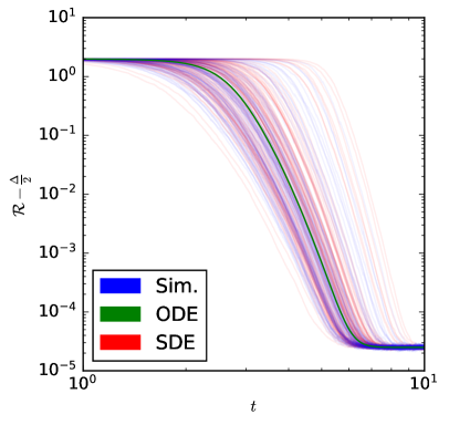
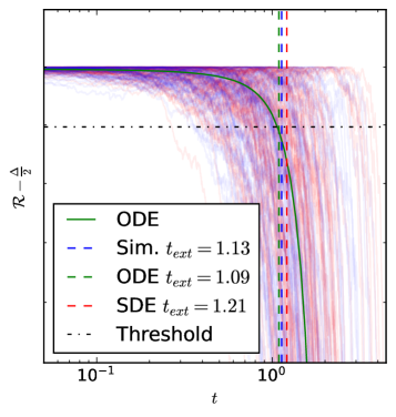
Figure 1: multiple run of the simulated SGD and the numerically integrated SDE, always starting from the same initial condition, with $d=3000$. All the $t_{\text{ext}}$ presented are obtained by solving numerically (21). The SDE captures the variance that the ODE doesn’t exhibit, but the $t_{\text{ext}}$ do not change considerably.

Notice that the stochastic correction is proportional to $\sqrt{\nicefrac{{\gamma}}{{d}}}$, consistent to a first order correction to the deterministic limit. Similarly to the discussion in Section 3.2, the spherical constraint can be imposed by projecting the process in the sphere. This is discussed in detail in App. B, and for $p=1$ reads:

$$\begin{split}\mathinner{\dfrac{\operatorname{d\!}{}m_{1}}{\operatorname{d\!}{t}}}&=\left(\Psi_{1}{(\mathrm{\Omega})}-\frac{m_{1}}{2}\Phi_{11}{(\mathrm{\Omega})}\right)\operatorname{d\!}t+\sqrt{\frac{\gamma}{d}}\,\left(\sigma_{m}-\frac{m_{1}}{2}\sigma_{Q}\right)\cdot\operatorname{d\!}B_{t}\end{split}$$ (27)

Figure 1 compares different instances of finite size simulations with instances of the SDE (27) with the same initial condition. Although the stochastic correction offers a better description of the process at large but finite dimensions, we find that quite surprisingly they have a small impact in the exit time. Hence, the formulas (22) & (23) derived in the Section 3.2 for random initialization provide a good approximation to the exit time. In Appendix  D we discuss how to derive an exit time formula with the stochastic corrections. As just showed, the new formulas do not offer any improvements compared to the deterministic ones, nevertheless the SDE could be useful in some particular and unrealistic nationalizations, since ODEs can fail.

To summarize, in this section we have shown that the deterministic ODEs provides a good approximation for the precise number of samples required for escaping mediocrity in high-dimensions. In other words, stochasticity does not help in navigating the flat directions at initalization and correlating with the signal.

4 The role of width

Thus far our discussion has focused on the well-specified case. We now discuss the role of width in escaping mediocrity. Our starting point are the deterministic ODEs (11) for the sufficient statistics derived in Section 2. As in our previous analysis, we focus on the spherical setting where $w_{i}\in\mathbb{S}^{d-1}(\sqrt{d})$, implying $Q_{jj}=1$, see Appendix B for a detailed derivation. First, we derive analytical expressions for the exit time for arbitrary width $p\geq 1$ in the particular case where the second layer is fixed at initialization $a^{0}_{j}=1$, $\forall j\in[n]$. The role played by the second layer is then discussed in Subsection 4.1.

Differently from the $p=1$ case, the process cannot be described be a single sufficient statistics, and instead we have to track $\nicefrac{{p(p-1)}}{{2}}$ non-diagonal entries of $Q$ (it is a symmetric matrix), and $p$ components of the vector $m$. Note that equation (21) remains valid to define $t_{\text{ext}}$, and can be solved numerically. An analytical expression for the exit time can be derived under similar assumptions to the ones discussed in Section 3.2, although the derivation is significantly more cumbersome. Full details can be found in Appendix  C. The final expressions for the annealed and quenched exit times are given by

$$t_{\text{ext}}^{\text{(anl)}}=\frac{\log\left[\frac{T(p+1)d+(p+1)(1-T)}{2p}\right]}{8\left[1-\frac{\gamma}{p}\left(1+\frac{1}{p}+\frac{4}{p^{2}}+\frac{\Delta}{2}\right)\right]}, t_{\text{ext}}^{\text{(qnc)}}=\mathbb{E}_{\mu_{0},\tau_{0}\sim\mathcal{P}^{d}_{p}}\left[\frac{\log\left[\frac{Tp(p+1)d+(2\mu_{0}p-\tau_{0})(1-T)}{2\mu_{0}p}\right]}{8\left[1-\frac{\gamma}{p}\left(1+\frac{1}{p}+\frac{4}{p^{2}}+\frac{\Delta}{2}\right)\right]}\right].$$ (28)

With the distribution of the variables $\tau_{0}$ and $\mu_{0}$ given by

$$\mu_{0},\tau_{0}\sim\mathcal{P}^{d}_{p}\quad\text{where }\mathcal{P}^{d}_{p}\equiv\left(d\sum_{j=1}^{p}(u_{j}\cdot v)^{2},2d\sum_{j=1}^{p}\sum_{l=j+1}^{p}(u_{j}\cdot u_{l})^{2}\right)\text{ with }v,u_{j}\sim\mathbb{S}^{d-1}(1).$$

Notice that $t_{\text{ext}}$ is a monotonically decreasing function of the width. Nevertheless, for any $p\geq 1$, the leading order dependence in the dimension is $t_{\text{ext}}=\log{d}$. Hence, despite helping escaping mediocrity, increasing the width cannot mitigate it. This can be contrasted to other aspects in which overparametrization can significantly help optimization, for instance with global convergence [48]. Interestingly, the minimal escaping time $t_{\text{ext}}^{\text{(anl)}}=\nicefrac{{1}}{{4}}\log(\nicefrac{{T(p+1)d+(p+1)(1-T)}}{{2p}})$, obtained by choosing the learning rate that minimizes the sample complexity for escaping, has the same pre-factor for any width $p\geq 1$, with the only differences being the dependence in $p$ inside the logarithm and in the time scaling $t=\nicefrac{{\nu\gamma}}{{pd}}$. At infinite width $p\to\infty$, this simply amounts to a factor $\frac{12+\Delta}{2+\Delta}$ with respect to $p=1$. Details of this computation can be found in Appendix C.4.

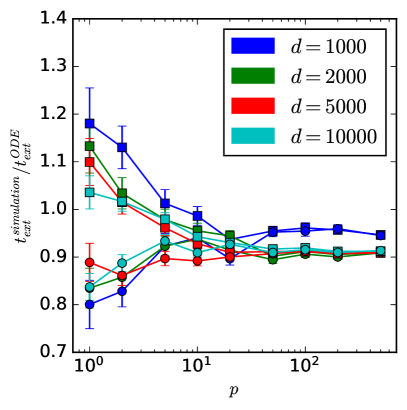
Figure 2: Ratio between the measured $t_{\text{ext}}$ from simulations and the corresponding analytical formula (square = annealed, circle = quenched). We average over many initial conditions, for different values of $p$. The ratio $\nicefrac{{\gamma}}{{p}}$ has been kept constant for different simulations.

Figure 2 compares our analytical formulas (28) with real one-pass SGD simulations. The simulation are averaged over many different instance of the initial conditions, and the ratio $\nicefrac{{\gamma}}{{p}}$ is kept constant when varying $p$, for not having discrepancies due to the different learning rate scaling. It’s interesting to notice how the two different formulas gives the same outcome for large width $p\gg 1$. Moreover, for narrow networks they essentially differ from by a $d$ independent constant. Figure 2 also suggests that, as for $p=1$, the stochasticity can be neglected in the estimation of the exit time. In Appendix E we provide further evidence of that.

4.1 Training the second layer

In the previous section, we have derived analytical expressions for the exit time in the particular case of fixed first layer weights $a^{0}_{j}=1$. Here, we provide numerical evidence that training the first layer does not significantly change our conclusions.

The key challenge is that by training the first layer we can’t measure $t_{\text{ext}}$ as the time needed to escape the risk at initialization. Indeed, from equation (21) it can be seen that in the very first steps of the learning the vector $a$ changes slightly to adapt to the initial conditions, thereby fitting the noise. In this scenario, instead of looking directly at the risk, we can instead use the largest component of the correlation vector $m$ as a measure on how much the network has learned. At random initialization, this is of order $\nicefrac{{1}}{{\sqrt{d}}}$, grows to $1$ as the neural network correlates with the target weights. A natural choice for initializing the second layer weights is $a^{0}_{j}=1$, $\forall j\in[p]$. In principle, this initial condition guarantees that the risk at initialization is exactly equal to the case where $a_{j}$ is fixed. On the other hand, as we already point out, the initial plateau where the dynamics gets stuck depends on the particular first layer initial condition. Even for other choices of initialization, e.g. $a_{j}\sim\text{Bernoulli}(\nicefrac{{1}}{{2}})$, the dynamics quickly goes the a plateau, so it does not really matter which $a_{j}^{0}$ is used. Therefore, for simplicity we choose an homogeneous initialization $a^{0}_{j}=1$. Figure 3 compares the evolution of the maximum correlation when learning the second layer or not, for different values of $p$.

It is important to stress that we are not claiming that the time needed to reach the minimum of the population risk is the same when training or not the second layer, as can be seen in Fig. 3. Instead, our result highlights that the time needed to escape the flat directions at initialization are close. In fact, after the two layer neural network has escaped mediocrity, the dynamics can be very different whether the second layer weights are trained or not. For instance, $a$ could become sparse with just a few neurons contributes to the output, or it could remain close to homogeneous $a_{j}=1$, and with all neurons correlating with the target. Although studying the dynamics after escaping mediocrity is surely an interesting endeavor, it’s out of the scope of this manuscript.

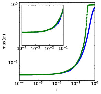
Figure 3: $p=20$ (left), $p=50$ (right), $d=1000$. Comparison between the growth of $\max{m}$ throughout the learning process, when the second layer is fixed (blue) and trained (green). The dynamics is obviously different far from the starting point, but when we zoom close to the exit point, the two processes have the same behavior, $t_{\text{ext}}$ included.

5 Conclusion

In this work we have derived a sharp formula for how many samples are required for a two-layer neural network trained with one-pass SGD to learn a quadratic target in the high-dimensional limit. In particular, we have shown that increasing the width can only improve the sample complexity by a pre-factor, with the overall scaling with the dimension remaining of the same order $n=O(d\log{d})$. Therefore, for this target overparametrization does not significantly help optimization, providing a prototypical example of a hard class of functions for learning with SGD. Our results rely on a low-dimensional description of SGD in terms of a stochastic process describing the evolution of the sufficient statistics in the high-dimensional limit. Surprisingly, we have shown that deriving the sample complexities from the deterministic drift of this process with small initial correlation with the target provides a fairly good approximation of the exit time as computed from the full process with zero initial correlation, showing stochasticity does not play a crucial role in escaping mediocrity for this problem.

Appendix A Explicit ODEs derivation

A.1 Derivation of the process

Let’s start by reminding the definition of displacement at step $\nu$

$$\mathcal{E}^{\nu}\coloneqq\frac{1}{p}\sum_{j=1}^{p}a_{j}(\lambda_{j}^{\nu})^{2}-(\lambda_{\star}^{\nu})^{2}+\sqrt{\Delta}z^{\nu},$$ (29)

from which it’s easy to write the loss function

$$\ell{(y^{\nu},f_{\Theta^{\nu}}(x^{\nu}))}=\frac{1}{2}\left(\mathcal{E}^{\nu}\right)^{2}.$$ (30)

The gradient respect to the parameters is given

$$\begin{split}\partial_{a_{j}}\ell{(y^{\nu},f_{\Theta^{\nu}}(x^{\nu}))}&=\frac{1}{p}\mathcal{E}^{\nu}(\lambda_{j}^{\nu})^{2}\\ \nabla_{w_{j}}\ell{(y^{\nu},f_{\Theta^{\nu}}(x^{\nu}))}&=\frac{1}{p}\mathcal{E}^{\nu}2a^{\nu}_{j}\lambda_{j}^{\nu}x^{\nu}\end{split}$$ (31)

Using $\gamma$ as learning rate for the weights $w_{j}$ and $\nicefrac{{\gamma}}{{p}}$ for the second layer, we have the following update equations

$$\begin{split}a^{\nu+1}_{j}&=a^{\nu}_{j}-\frac{\gamma}{pd}\mathcal{E}^{\nu}(\lambda_{j}^{\nu})^{2}\\ w_{j}^{\nu+1}&=w_{j}^{\nu}-\frac{\gamma}{p}\mathcal{E}^{\nu}2a^{\nu}_{j}\lambda_{j}^{\nu}x^{\nu}\end{split}$$ (32)

Applying the definition of the sufficient statistics, $m_{j}=\nicefrac{{w_{j}w^{\star}}}{{d}}$ and $Q_{jl}=\nicefrac{{w_{j}w_{l}}}{{d}}$, we can recover Eqs. (7).

A.2 Explicit ODE

To get the explicit form of our ODEs we need to compute some expected value over the preactivations $(\lambda_{\star},\lambda)$. These are gaussian variables, whose correlation matrix is given by $\Omega$. Similarly, the population risk is defined as

$$\mathcal{R}=\mathbb{E}_{(\lambda,\lambda^{\star})\sim\mathcal{N}(0_{p+1},\Omega)}\left[\frac{1}{2}\mathcal{E}^{2}\right].$$

Let’s look close to the random variable we need for this expected values, expressing them just as function of local fields. To be more concise, from now on with $\mathbb{E}$ we always mean the expected value over $(\lambda,\lambda^{\star})\sim\mathcal{N}(0_{p+1},\Omega)$. For the risk we just need

$$\begin{split}\mathbb{E}\left[\mathcal{E}^{2}\right]=&\lambda_{\star}^{4}+\frac{1}{p^{2}}\sum_{j,l=1}^{p}a_{j}a_{l}\mathbb{E}\left[\lambda_{j}^{2}\lambda_{l}^{2}\right]-\frac{2}{p}\sum_{j=1}^{p}a_{j}\mathbb{E}\left[\lambda_{j}^{2}\lambda_{\star}^{2}\right],\end{split}$$

while for the ODE of $\bar{a}$

$$\begin{split}\mathbb{E}\left[\mathcal{E}\lambda_{j}^{2}\right]=\frac{1}{p}\sum_{l=1}^{p}a_{l}\mathbb{E}\left[\lambda_{l}^{2}\lambda_{j}^{2}\right]-\mathbb{E}\left[\lambda_{\star}^{2}\lambda_{j}^{2}\right],\end{split}$$

where we omitted the noise part since it averages out with the expectation. The equation for $\bar{m}$ requires

$$\begin{split}2a_{j}\mathbb{E}\left[\mathcal{E}\lambda_{j}\lambda_{\star}\right]=\frac{2}{p}\sum_{l=1}^{p}a_{j}a_{l}\mathbb{E}\left[\lambda_{l}^{2}\lambda_{j}\lambda_{\star}\right]-2\mathbb{E}\left[\lambda_{\star}^{2}\lambda_{j}\lambda_{\star}\right],\end{split}$$

while we need two different expectations for $\bar{Q}$

$$\begin{split}2(a_{j}+a_{l})\mathbb{E}\left[\mathcal{E}\lambda_{j}\lambda_{\star}\right]&=2(a_{j}+a_{l})\left[\frac{1}{p}\sum_{s=1}^{p}a_{s}\mathbb{E}\left[\lambda_{s}^{2}\lambda_{j}\lambda_{l}\right]-\mathbb{E}\left[\lambda_{\star}^{2}\lambda_{j}\lambda_{l}\right]\right]\quad\text{and}\\ 4\frac{\gamma}{p}{\mathcal{E}}^{2}a_{j}a_{l}\lambda_{j}\lambda_{l}=16\frac{\gamma}{p}a_{j}a_{l}\Bigg{[}&\mathbb{E}\left[\lambda_{j}\lambda_{l}\lambda_{\star}^{4}\right]-\frac{2}{p}\sum_{s=1}^{p}a_{s}\mathbb{E}\left[\lambda_{j}\lambda_{l}\lambda_{\star}^{2}\lambda_{s}^{2}\right]+\frac{1}{p^{2}}\sum_{s,t=1}^{p}\left(a_{s}a_{t}\mathbb{E}\left[\lambda_{j}\lambda_{l}\lambda_{s}^{2}\lambda_{t}^{2}\right]+\Delta\mathbb{E}\left[\lambda_{j}\lambda_{l}\right]\right)\Bigg{]}.\end{split}$$

We are left to compute some distribution moments of a multivariate Gaussian of second, fourth and sixh order. In the GitHub repository can be found a Mathematica script to address this task; alternatively Isserlis’ Theorem can be applied. We introduce a shorthand in the notation

$$\omega_{\alpha\beta}\coloneqq\left[{\Omega}\right]_{\alpha\beta},$$

where the indices $\alpha$ and $\beta$ can discriminate between local fields $\lambda$ (if $\alpha,\beta\in[1,\dots,p]$, and $\lambda_{\star}$ (if $\alpha,\beta=p+1$). The final result are given by

$$\mathbb{E}\left[\lambda_{\alpha}\lambda_{\beta}\right] =\omega_{\alpha\beta}$$

$$\mathbb{E}\left[\lambda_{\alpha}^{2}\lambda_{\beta}^{2}\right] =\omega_{\alpha\alpha}\omega_{\beta\beta}+2\omega_{\alpha\beta}^{2}$$

$$\mathbb{E}\left[\lambda_{\alpha}\lambda_{\beta}\lambda_{\gamma}^{2}\right] =\omega_{\alpha\beta}\omega_{\gamma\gamma}+2\omega_{\alpha\gamma}\omega_{\beta\gamma}$$

$$\mathbb{E}\left[\lambda_{\alpha}\lambda_{\beta}\lambda_{\gamma}^{2}\lambda_{\delta}^{2}\right] =\omega_{\alpha\beta}\omega_{\gamma\gamma}\omega_{\delta\delta}+2\omega_{\alpha\beta}\omega_{\gamma\delta}^{2}+2\omega_{\alpha\gamma}\omega_{\beta\gamma}\omega_{\delta\delta}+$$

$$\quad 4\omega_{\alpha\gamma}\omega_{\beta\delta}\omega_{\gamma\delta}+4\omega_{\alpha\delta}\omega_{\beta\gamma}\omega_{\gamma\delta}+2\omega_{\alpha\delta}\omega_{\beta\delta}\omega_{\gamma\gamma}$$

By retracing all steps backward and making the necessary substitutions, we can arrive at an explicit form of the ODEs and population risk. While the full risk expression can be found in Eq. (6), we report here just the case $a_{j}=1$ for the ODEs since they have a compact matrix form

$$\mathinner{\dfrac{\operatorname{d\!}{}m}{\operatorname{d\!}{t}}} =2\left(\rho-\frac{\operatorname{Tr}{\left[Q\right]}}{p}\right)m+4\left(\rho m-\frac{Qm}{p}\right)$$ (33a)

$$\begin{split}\mathinner{\dfrac{\operatorname{d\!}{}Q}{\operatorname{d\!}{t}}}&=4\left(\rho-\frac{\operatorname{Tr}{\left[Q\right]}}{p}\right)Q+8\left(\frac{mm^{\top}}{k}-\frac{Q^{2}}{p}\right)\\ &\quad+\frac{4\gamma}{p}\Biggr{\{}\left[3\rho^{2}Q+12\rho mm^{\top}\right]+\frac{1}{p^{2}}\left[\left(\operatorname{Tr}{\left[Q\right]}^{2}+2\operatorname{Tr}{\left[Q^{2}\right]}\right)Q+4\operatorname{Tr}{\left[Q\right]}Q^{2}+8Q^{3}\right]\\ &\qquad\quad\quad-\frac{2}{p}\Biggl{[}\left(\rho\operatorname{Tr}{\left[Q\right]}+2\operatorname{Tr}{\left[mm^{\top}\right]}\right)Q+2\operatorname{Tr}{\left[Q\right]}mm^{\top}\\ &\qquad\qquad\qquad\quad+2\rho Q^{2}+4\left(mm^{\top}Q+Qmm^{\top}\right)\Biggl{]}+\Delta Q\Biggr{\}},\end{split}$$ (33b)

where $\rho\coloneqq\nicefrac{{w_{\star}^{2}}}{{d}}$. For completeness, this is Eq. (6) for the case $a_{j}=1$

$$\begin{split}\mathcal{R}(\Omega)\!=\!\frac{3+\Delta}{2}\!-\!\frac{\rho\operatorname{Tr}{\left[Q\right]}+2\operatorname{Tr}{\left[mm^{\top}\right]}}{p}\!+\!\frac{\operatorname{Tr}{\left[Q\right]}^{2}+2\operatorname{Tr}{\left[Q^{2}\right]}}{2p^{2}}.\end{split}$$ (34)

Appendix B Spherically constrainted ODE and SDE

B.1 Spherical constraint for ODE

Let’s recall the update rule for the weights

$$w_{j}^{\nu+1}=\frac{w_{j}^{\nu}-\gamma\nabla_{w_{j}}\ell(y^{\nu},f_{\Theta^{\nu}}(x^{\nu}))}{\left\lVert w_{j}^{\nu}-\gamma\nabla_{w_{j}}\ell(y^{\nu},f_{\Theta^{\nu}}(x^{\nu}))\right\rVert}\sqrt{d},$$ (35)

we will find the leading order approximation of it and then apply the argument as the unconstrained case for deriving the ODEs. To shorten the notation we will use $\ell^{\nu}$ for indicating $\ell(y^{\nu},f_{\Theta^{\nu}}(x^{\nu}))$.

Let’s start by computing the normalization factor

$$\begin{split}\frac{1}{\left\|w^{\nu}_{j}-\gamma\nabla_{w_{j}}{\ell^{\nu}}\right\|}=&\left[\left(w^{\nu}_{j}-\gamma\nabla_{w_{j}}{\ell^{\nu}}\right)\cdot\left(w^{\nu}_{j}-\gamma\nabla_{w_{j}}{\ell^{\nu}}\right)\right]^{-\frac{1}{2}}\\ =&\left[\left\|w^{\nu}_{j}\right\|^{2}-2\gamma w^{\nu}_{j}\cdot\nabla_{w_{j}}{\ell^{\nu}}+\gamma^{2}\left\|\nabla_{w_{j}}{\ell^{\nu}}\right\|^{2}\right]^{-\frac{1}{2}}\\ =&\frac{1}{\sqrt{d}}\left[1-\frac{1}{d}\left(2\gamma w^{\nu}_{j}\cdot\nabla_{w_{j}}{\ell^{\nu}}-\gamma^{2}\left\|\nabla_{w_{j}}{\ell^{\nu}}\right\|^{2}\right)\right]^{-\frac{1}{2}}\\ =&\frac{1}{\sqrt{d}}\left[1+\frac{1}{2d}\left(2\gamma w^{\nu}_{j}\cdot\nabla_{w_{j}}{\ell^{\nu}}-\gamma^{2}\left\|\nabla_{w_{j}}{\ell^{\nu}}\right\|^{2}\right)+o\left(d^{-1}\right)\right].\end{split}$$

Note that we kept both two terms in the expansion because we can show that both the norm and the scalar product with a weight vector are order 1

$$\begin{split}\left\|\nabla_{w_{j}}{\ell^{\nu}}\right\|^{2}\sim&\frac{2\mathcal{E}^{2}\lambda^{\nu}_{j}}{p^{2}}\frac{\sum_{i=1}^{d}\left(x^{\nu}_{i}\right)^{2}}{d}\sim\frac{2\mathcal{E}^{2}\lambda^{\nu}_{j}}{p^{2}}\frac{\chi^{2}_{d}}{d}=\mathcal{O}\left(1\right),\\ w_{j}\cdot\nabla_{w_{l}}{\ell^{\nu}}\sim&\frac{2\mathcal{E}\lambda^{\nu}_{l}}{p}\sum_{i=1}^{d}\frac{w_{j,i}}{\sqrt{d}}\mathcal{N}{(0,1)}\sim\frac{2\mathcal{E}\lambda^{\nu}_{l}}{p^{2}}\mathcal{N}{\left(0,\sum_{i=1}^{d}\frac{w^{2}_{j,i}}{d}\right)}\sim\frac{2\mathcal{E}\lambda^{\nu}_{l}}{p^{2}}\mathcal{N}{\left(0,1\right)}=\mathcal{O}\left(1\right).\end{split}$$

We can now plug the expansion back into the original update rule

$$w^{\nu+1}_{j}=\left(w^{\nu}_{j}-\gamma\nabla_{w_{j}}{\ell^{\nu}}\right)\left[1+\frac{1}{2d}\left(2\gamma w^{\nu}_{j}\cdot\nabla_{w_{j}}{\ell^{\nu}}-\gamma^{2}\left\|\nabla_{w_{j}}{\ell^{\nu}}\right\|^{2}\right)+o\left(d^{-1}\right)\right]\sqrt{d}.$$

We are ready to go over the steps that take us from the update rule on vector weights to those on order parameters. We report by way of example the steps performed for $m$; the accounts for $Q$ are similar, just a bit more tedious.

$$\begin{split}m^{\nu+1}_{j}&=\frac{w^{\nu+1}_{j}\cdot w^{*}}{d}\\ &=\left(m^{\nu}_{j}-\frac{\gamma w^{*}\cdot\nabla_{w_{l}}{\ell^{\nu}}}{d}\right)\left[1+\frac{1}{2d}\left(2\gamma w^{\nu}_{j}\cdot\nabla_{w_{j}}{\ell^{\nu}}-\gamma^{2}\left\|\nabla_{w_{j}}{\ell^{\nu}}\right\|^{2}\right)+o\left(d^{-1}\right)\right]\\ &=m^{\nu}_{j}-\frac{\gamma w^{*}\cdot\nabla_{w_{l}}{\ell^{\nu}}}{d}+\frac{m^{\nu}_{jr}}{2d}\left(2\gamma w^{\nu}_{j}\cdot\nabla_{w_{j}}{\ell^{\nu}}-\gamma^{2}\left\|\nabla_{w_{j}}{\ell^{\nu}}\right\|^{2}\right)+o\left(d^{-1}\right)\\ &=m^{\nu}_{j}+\frac{1}{d}\left[\frac{\gamma}{p}\lambda^{\star}\mathcal{E}^{\nu}\lambda^{\nu}_{j}-\frac{m^{\nu}_{j}}{2}\left(2\frac{\gamma}{p}\mathcal{E}^{\nu}\lambda^{\nu}_{j}\lambda^{\nu}_{j}+\frac{\gamma^{2}}{p^{2}}{\mathcal{E}^{\nu}\lambda^{\nu}_{j}}^{2}\right)\right]+o\left(d^{-1}\right).\end{split}$$ (36)

We can now take the limit $d\to+\infty$, claiming that the theorem [19, 16] proving ODE convergence is still valid. Indeed, the error term $o(d^{-1})$ in Eq. (36) has an average order of $O(d^{-2})$, which can be absorbed in the term $\Gamma^{\nu}$ of Theorem A.1 in [19]. The rest of the proof proceeds the same way, noting that the square function can be assumed to be Lipschitz since the dynamics take place on the sphere.

The differential equation that describes the evolution of $m$ is

$$\mathinner{\dfrac{\operatorname{d\!}{}\bar{m}_{j}{\left(t\right)}}{\operatorname{d\!}{t}}}=\mathbb{E}_{\lambda,\lambda^{*}\sim\mathcal{N}{(0,\Omega{(t)})}}{\left[2\mathcal{E}\lambda_{j}\lambda_{\star}-\frac{\bar{m}_{j}{\left(t\right)}}{2}\left(4\mathcal{E}\lambda_{j}\lambda_{j}+4\frac{\gamma}{p}{\mathcal{E}}^{2}\lambda_{j}^{2}\right)\right]};$$

Using the definitions introduced in Equations (15) we can write the equation in a nicer form

$$\mathinner{\dfrac{\operatorname{d\!}{}\bar{m}_{j}{\left(t\right)}}{\operatorname{d\!}{t}}}=\Psi_{j}{(\Omega)}-\frac{\bar{m}_{j}{\left(t\right)}}{2}\Phi_{jj}{(\Omega)}.$$ (37)

Essentially, the spherical constraint can be imposed by using a term proportional to the unconstrained $Q$ update.

Without reporting all the calculations, we can write an analogous differential equation for $Q$ evolution

$$\mathinner{\dfrac{\operatorname{d\!}{}\bar{Q}_{jl}{\left(t\right)}}{\operatorname{d\!}{t}}}=\Phi_{jl}{(\Omega)}-\frac{\bar{Q}_{jl}{\left(t\right)}}{2}\left(\Phi_{jj}{(\Omega)}+\Phi_{ll}{(\Omega)}\right).$$ (38)

Note that $\mathinner{\dfrac{\operatorname{d\!}{}\bar{Q}_{jj}{\left(t\right)}}{\operatorname{d\!}{t}}}=0$ if $Q_{jj}{\left(t\right)}=1$, as it should be since the norm of spherical vectors must not change.

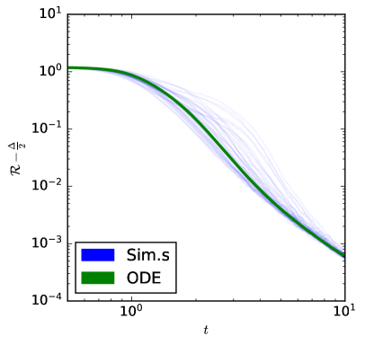
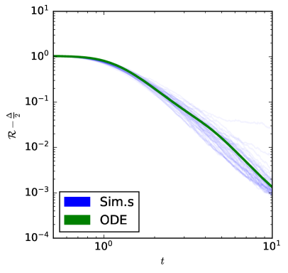
Figure 4: comparison of ODE integration and many SGD runs for $p=5$ (left) and $p=20$ (right). Both the experiments have $d=5000$.

In Figure 4 we show two examples of integration of ODEs, for different values of $p$. Simulating for large but finite $d$ does not kills the stochasticity in the SGD runs, but we can clearly see how the ODE well describe the dynamics on average.

B.2 Spherical constraint for SDE

This subsection we derive the spherical constraint for the SDE, with $p=1$. We assume that the stochastic process is given

$$\begin{split}\operatorname{d\!}m&=\Psi_{1}{(\Omega)}\operatorname{d\!}t+\sqrt{\frac{\gamma}{d}}\,\sigma_{m}{(\Omega)}\cdot\operatorname{d\!}B_{t}\\ \operatorname{d\!}Q&=\Phi_{11}{(\Omega)}\operatorname{d\!}t+\sqrt{\frac{\gamma}{d}}\,\sigma_{Q}{(\Omega)}\cdot\operatorname{d\!}B_{t},\end{split}$$ (39)

without providing explicit expressions for $\sigma_{m}{(\Omega)}$ and $\sigma_{Q}{(\Omega)}$; see Appendix E for that.

The derivation is basically following the steps of the previous Section. Starting from the unconstrainted update rule for the weights

$$w^{\nu+1}_{j}=w^{\nu}_{j}-\gamma\nabla_{w_{j}}{\ell^{\nu}},$$

we can find an expression for the two unconstrained differentials

$$\begin{split}\operatorname{d\!}q&=\frac{-2\gamma w\cdot\nabla{\ell^{\nu}}+\gamma^{2}\left\|\nabla{\ell^{\nu}}\right\|^{2}}{d}\\ \operatorname{d\!}m&=\frac{-\gamma w_{\star}\cdot\nabla\ell^{\nu}}{d}.\end{split}$$ (40)

Since we are forcing the weight on the sphere, the update rule that actually has to be used is

$$w^{\nu+1}_{j}=\frac{w^{\nu}_{j}-\gamma\nabla_{w_{j}}{\ell^{\nu}}}{w^{\nu}_{j}-\gamma\nabla_{w_{j}}{\ell^{\nu}}}\sqrt{d};$$

multiplying both sides by $w_{\star}$ and subtracting $m$ we get

$$\operatorname{d\!}m_{S}=\frac{m+\operatorname{d\!}m}{\left\|w-\gamma\nabla{\ell^{\nu}}\right\|}\sqrt{d}-m,$$

where we introduce $m_{S}$ to differentiate the constrained variable from $m$. Let’s estimate the normalization factor

$$\begin{split}\left\|w-\gamma\nabla{\ell^{\nu}}\right\|=&\sqrt{(w-\gamma\nabla{\ell^{\nu}})^{2}}=\sqrt{w^{2}-2w\cdot\gamma\nabla{\ell^{\nu}}+\gamma^{2}\left\|\nabla{\ell^{\nu}}\right\|^{2}}\\ =&\sqrt{d}\sqrt{\frac{w^{2}}{d}+\frac{-2w\cdot\gamma\nabla{\ell^{\nu}}+\gamma^{2}\left\|\nabla{\ell^{\nu}}\right\|^{2}}{d}}=\sqrt{d}\sqrt{q+\operatorname{d\!}q}\\ =&\sqrt{d}\sqrt{1+\operatorname{d\!}q},\end{split}$$

where in the last step we used the constraint $q=1$. We can now plug it back in $\operatorname{d\!}m_{S}$

$$\operatorname{d\!}m_{S}=\frac{m+\operatorname{d\!}m}{\sqrt{1+\operatorname{d\!}q}}-m,$$

and expanding up to leading orders we get

$$\begin{split}\operatorname{d\!}m_{S}=&(m+\operatorname{d\!}m)(1+\operatorname{d\!}q)^{-\frac{1}{2}}-m=(m+\operatorname{d\!}m)\left(1-\frac{1}{2}\operatorname{d\!}q+\frac{3}{8}\operatorname{d\!}q^{2}\right)-m\\ =&\operatorname{d\!}m-\frac{m}{2}\operatorname{d\!}q-\frac{1}{2}\operatorname{d\!}m\operatorname{d\!}q+\frac{3}{8}m\operatorname{d\!}q^{2}\end{split}$$

In principle, we can now use the Itô Lemma on differentials Equations (39), obtaining

$$\operatorname{d\!}m^{2}=\frac{\gamma}{d}\sigma_{m}^{2}{(\Omega)}\operatorname{d\!}t,\quad\operatorname{d\!}q^{2}=\frac{\gamma}{d}\sigma^{2}_{m}{(\Omega)}\operatorname{d\!}t,\quad\text{and}\quad\operatorname{d\!}m\operatorname{d\!}q=\frac{\gamma}{d}\sigma_{m}{(\Omega)}\cdot\sigma_{Q}{(\Omega)}\operatorname{d\!}t.$$

It’s interesting to note that these lead to a drift correction (and not just stochastic), but it’s of second order. As expected, in numerical simulations we can’t see the effect for these corrections, hence we neglet them in what follows. Finally, we write the explicit Brownian motion for the constrained dynamic

$$\operatorname{d\!}m_{S}=\left(\Psi_{1}{(\Omega)}-\frac{m_{S}}{2}\Phi_{11}{(\Omega)}\right)\operatorname{d\!}t+\sqrt{\frac{\gamma}{d}}\left(\sigma_{m}{(\Omega)}-\frac{m_{S}}{2}\sigma_{Q}{(\Omega)}\right)\cdot\operatorname{d\!}B_{t}.$$ (41)

Of course, all functions depending on $\Omega$ should be evaluated at $m=m_{S},q=1$.

Appendix C Derivation of the expected exit time formulas

C.1 Linearization of the equations

The linear approximation of $\Psi$ around $m_{j}\approx 0$ is given by

$$\Psi_{j}=4\left(m_{j}-\frac{m_{j}}{p}\right)=4\left(1-\frac{1}{p}\right)m_{j},$$ (42)

while for $\Phi$ we distinguish the cases $j=l$ or not

$$\begin{split}j\neq l\quad\Phi_{jl}&=4\left[2\left(-2\frac{Q_{jl}}{p}\right)\right]+\\ &\quad+\frac{4\gamma}{p}\Biggr{\{}3Q_{jl}-\frac{2}{p}\Biggl{[}pQ_{jl}+4Q_{jl}\Biggl{]}+\frac{1}{p^{2}}\left[\left(p^{2}+2p\right)Q_{jl}+8pQ_{jl}+24Q_{jl}\right]+\Delta Q_{jl}\Biggr{\}}\\ &=-\frac{16}{p}Q_{jl}+\frac{4\gamma}{p}\left\{3-2-\frac{8}{p}+1+\frac{2}{p}+\frac{8}{p}+\frac{24}{p^{2}}+\Delta\right\}Q_{jl}\\ &=-\frac{16}{p}Q_{jl}+\frac{4\gamma}{p}\left\{2+\frac{2}{p}+\frac{24}{p^{2}}+\Delta\right\}Q_{jl}\end{split}$$ (43)

$$\begin{split}j=l\quad\Phi_{jj}&=4\left[2\left(-\frac{1}{p}\right)\right]+\frac{4\gamma}{p}\Biggr{\{}3-\frac{2}{p}\Biggl{[}p+2\Biggl{]}+\frac{1}{p^{2}}\left[\left(p^{2}+2p\right)+4p+8\right]+\Delta\Biggr{\}}\\ &=-\frac{8}{p}+\frac{4\gamma}{p}\left\{3-2-\frac{4}{p}+1+\frac{2}{p}+\frac{4}{p}+\frac{8}{p^{2}}+\Delta\right\}\\ &=-\frac{8}{p}+\frac{4\gamma}{p}\left\{2+\frac{2}{p}+\frac{8}{p^{2}}+\Delta\right\}\end{split}$$ (44)

Given these linear approximations, we are ready to write down the equations valid as long as the risk stays in the first plateau

$$\begin{split}\mathinner{\dfrac{\operatorname{d\!}{}\left[m{\left(t\right)}\right]_{j}}{\operatorname{d\!}{t}}}&=\left[4\left(1-\frac{1}{p}\right)+\frac{4}{p}-\frac{2\gamma}{p}\left(2+\frac{2}{p}+\frac{8}{p^{2}}+\Delta\right)\right]\left[m{\left(t\right)}\right]_{j}\\ &=\left[4-\frac{2\gamma}{p}\left(2+\frac{2}{p}+\frac{8}{p^{2}}+\Delta\right)\right]\left[m{\left(t\right)}\right]_{j}\\ &=4\left[1-\frac{\gamma}{p}\left(1+\frac{1}{p}+\frac{4}{p^{2}}+\frac{\Delta}{2}\right)\right]\left[m{\left(t\right)}\right]_{j},\end{split}$$ (45)

$$\begin{split}\mathinner{\dfrac{\operatorname{d\!}{}\left[Q{\left(t\right)}\right]_{jl}}{\operatorname{d\!}{t}}}&=\left[-\frac{16}{p}+\frac{4\gamma}{p}\left(2+\frac{2}{p}+\frac{24}{p^{2}}+\Delta\right)+\frac{8}{p}-\frac{4\gamma}{p}\left(2+\frac{2}{p}+\frac{8}{p^{2}}+\Delta\right)\right]\left[Q{\left(t\right)}\right]_{jl}\\ &=\left[-\frac{8}{p}+\frac{4\gamma}{p}\left(\frac{16}{p^{2}}\right)\right]\left[Q{\left(t\right)}\right]_{jl}\\ &=-\frac{8}{p}\left[1-\frac{8\gamma}{p^{2}}\right]\left[Q{\left(t\right)}\right]_{jl}.\end{split}$$ (46)

We observe that the evolution of the sufficient statistics is uncoupled in the starting saddle. We can shorthand the notation by introducing $\omega_{Q}$ and $\omega_{M}$

$$\begin{split}\mathinner{\dfrac{\operatorname{d\!}{}m_{j}}{\operatorname{d\!}{t}}}&=\omega_{M}m_{j}\\ \mathinner{\dfrac{\operatorname{d\!}{}Q_{jl}}{\operatorname{d\!}{t}}}&=-\omega_{Q}Q_{jl}\quad\text{when }j\neq l.\end{split}$$ (47)

These equations admit a simple solution given by

$$\begin{split}m_{j}{(t)}&=m_{j}{(0)}\exp[\omega_{M}t]\\ Q_{jl}{(t)}&=Q_{jl}{(0)}\exp[-\omega_{Q}t].\end{split}$$ (48)

C.2 Solving the approximated risk equation

From Eq. (34) when the weights are on the sphere, it follows that the risk is given by

$$\mathcal{R}{(Q,m)}-\frac{\Delta}{2}=1+\frac{1}{p}+\frac{1}{p^{2}}\sum_{j,l=1;j\neq l}^{p}Q^{2}_{jl}-\frac{2}{p}\sum_{j=1}^{p}m^{2}_{j}$$ (49)

Eqs. (48) can be used to obtain a deterministic time evolution of the risk. The only source of randomness left is from the initial conditions, we can define two random variables as

$$\frac{\mu_{0}}{d}\coloneqq\sum_{j=1}^{p}\left[m_{j}(0)\right]^{2}\quad\text{and}\quad\frac{\tau_{0}}{d}\coloneqq\sum_{j,l=1;j\neq l}^{p}\left[Q_{jl}(0)\right]^{2},$$ (50)

and get an expression for the risk in function of time

$$\mathcal{R}(t)-\frac{\Delta}{2}=1+\frac{1}{p}+\frac{d\tau_{0}}{p^{2}}\exp[-2\omega_{Q}t]-\frac{2d\mu_{0}}{p}\exp[2\omega_{M}t]$$ (51)

This equation is not polished enough to be solved analytically yet. First of all we need to assume that the risk is decreasing by forcing $\omega_{m}>0$. Secondly, we want the exponential proportional to $\tau_{0}$ to be negligible when $t>0$: this follow from $\omega_{Q}>0$. In principle, this last condition is not needed for the process to converge like the first one, but without it is not possible to find an analytical solution for the cross -threshold equation. Moreover, when $p>6$: $\omega_{m}>0\implies\omega_{Q}>0$, so we can see that the request is not unreasonable.

Wrapping all this consideration together, Eq. (21) is

$$(1-T)\left(1+\frac{1}{p}+\frac{\tau_{0}}{dp^{2}}-\frac{2\mu_{0}}{dp}\right)=1+\frac{1}{p}-\frac{2\mu_{0}}{dp}\exp[2\omega_{M}t_{\text{ext}}],$$ (52)

from where we can compute the exit time

$$t_{\text{ext}}=\frac{\log\left[\frac{Tp(p+1)d+(2\mu_{0}p-\tau_{0})(1-T)}{2\mu_{0}p}\right]}{2\omega_{m}}.$$

C.3 Averaging on initial conditions

As of now $t_{\text{ext}}$ is still depending on the initial conditions through the random variables $\mu_{0}$ and $\tau_{0}$. Following from the choosen initial conditions, and taking into account the dependence between the two random variables

$$\mu_{0},\tau_{0}\sim\mathcal{P}^{d}_{p}\quad\text{where }\mathcal{P}^{d}_{p}\equiv\left(d\sum_{j=1}^{p}(u_{j}\cdot v)^{2},2d\sum_{j=1}^{p}\sum_{l=j+1}^{p}(u_{j}\cdot u_{l})^{2}\right)\text{ with }v,u_{j}\sim\mathbb{S}^{d-1}(1).$$

We have now two possibility to get the expectation of $t_{\text{ext}}$. The first one is known in statistical physics literature as quenched formula leaves us with an unexpressed expected value

$$t_{\text{ext}}^{\text{(qnc)}}=\mathbb{E}_{\mu_{0},\tau_{0}\sim\mathcal{P}^{d}_{p}}\left[\frac{\log\left[\frac{Tp(p+1)d+(2\mu_{0}p-\tau_{0})(1-T)}{2\mu_{0}p}\right]}{2\omega_{m}}\right].$$ (53)

The second one, often referred as the annealed formula, is obtain by simply replacing the random variables with their expected values

$$t_{\text{ext}}^{\text{(anl)}}=\frac{\log\left[\frac{T(p+1)d+(p+1)(1-T)}{2p}\right]}{2\omega_{m}}.$$ (54)

Case $p=1$

For completeness, let’s reduce these formulas to the simplest case $p=1$. In this case $\tau_{0}$ does not appear, and from Eq. (13) we find that $\mu_{0}\sim\chi^{2}(1)$, so the quenched formula reduces to

$$t_{\text{ext}}^{\text{(qnc)}}=\mathbb{E}_{\mu_{0}\sim\chi^{2}(1)}\left[\frac{\log\left[\frac{Td}{\mu_{0}}+(1-T)\right]}{8(1-6\gamma)-4\gamma\Delta)}\right].$$ (55)

C.4 Overparameterization Gain

Let introduce the number of gradient step needed to escape the threshold. Remembering $t=\nicefrac{{\nu\gamma}}{{pd}}$, we define

$$s_{\text{ext}}{(p,d,\gamma,\Delta,T)}\coloneqq\frac{pd}{\gamma}t_{\text{ext}}.$$ (56)

In the domain of our interest, namely $s_{\text{ext}}>0$, $s_{\text{ext}}$ is and convex function in $\gamma$. Therefore, it exist a unique minimum that correspond to the minimum number of steps required to cross the threshold when $p,d$ are fixed

$$0=\mathinner{\mathinner{\dfrac{\partial{}s_{\text{ext}}{(p,d,\gamma,\Delta,T)}}{\partial{\gamma}}}\Biggr{\rvert}}_{\gamma=\gamma_{\text{opt}}{(p,d,\Delta)}}\quad\implies\quad\gamma_{\text{opt}}{(p,d,\Delta)}=\frac{p^{3}}{8+2p+(2+\Delta)p^{2}}$$

Note that this learning rate correspond to an exit time whose log’s prefactor is constant to $\frac{1}{4}$, as reported in the main. We can also compute the optimal number of steps; we choose to stick with the annealed formula: for large $p$ both the estimation lead to the same result, while for small $p$ we are underestimating the exit time of a small factor. Hence, the annealed minimum number of steps is

$$s^{\text{min}}_{\text{ext}}{(p,d,\Delta,T)}\coloneqq s^{\text{anl}}_{\text{ext}}{(p,d,\gamma_{\text{opt}}{(p,d,\Delta)},\Delta,T)}=\frac{d\left[8+2p+(2+\Delta)p^{2}\right]\log\left[\frac{T(p+1)d+(p+1)(1-T)}{2p}\right]}{4p^{2}}.$$

This formula can be used to estimate the overparametrization gain. Noting that $s^{\text{min}}_{\text{ext}}$ is monotonically decrising in $p$, we can define the gain as

$$\lim_{d\to+\infty}\frac{s^{\text{min}}_{\text{ext}}{(p=1,d,\Delta,T)}}{\lim_{p\to+\infty}s^{\text{min}}_{\text{ext}}{(p,d,\Delta,T)}}=\frac{12+\Delta}{2+\Delta}.$$

Appendix D Stocastich correction to exit time formula

In this section we derive a new exit time formula for the case $p=1$, that takes into account the stochastic corrections of the dynamics.

At first, we require the further assumption $w^{0}\perp w_{\star}^{0}$. Obviously, this is not realistic, since to achieve this initialization we should know $w_{\star}$ exactly. Still, this case is could arise interest, since it corresponds to $m^{0}=0$, that is a fixed point of Equation (19). Thus, there is no dynamics in the ODE description, while the SDE are able to jump out from the fixed point and reach the point of convergence of the SGD. Lastly, the following analysis can be generalized to be used with the usual initial conditions.

The key observation is approximating both the noise and the drift of Equation (41) to the first non-zero order, when evaluated at $m=0$. As we pointed out above, the drift term is null at initialization, so the leading order is the first; this corresponds to the linearization of Equation (19), and the linear factor is

$$\mu\coloneqq\left[4(1-6\gamma)-2\gamma\Delta\right].$$ (57)

Instead, the noise term is not vanishing at $m=0$. Of course, $\sigma_{Q}{(\Omega)}$ does not contribute because is proportional to $m_{S}$. Moreover, looking at the expression for $\Sigma$ in Appendix E, we can observe that the covariance matrix is diagonal since the non-diagonal term is proportional to $m_{S}$ as well. All considered, the only term is contributing is the variance of $m$: the two-dimensional Brownian motion can be reduced to one in dimension 1, with variance

$$\sigma^{2}\coloneqq\frac{\gamma}{pd}(48+4\Delta).$$

Summarizing, the SDE near the initialization can be described as

$$\operatorname{d\!}m=\mu\operatorname{d\!}t+\sigma\operatorname{d\!}b_{t},$$ (58)

where $b_{t}$ is a one-dimensional Wiener process with unit variance. The approximated evolution of $m$ is a expansive Ornstein–Uhlenbeck process, since $\mu>0$. We have already shown in the main that there is a direct map between $m$ and the population risk; we can deal just with $m$ for measuring the exit time. Given an expansive OU-process staring at $m=0$, the mean first exit time from the interval $(-\sqrt{T},\sqrt{T})$ is given by [49]

$$t^{(SDE)}_{\text{ext}}=\frac{T}{\sigma^{2}}\prescript{}{2}{F}_{2}{\left(1,1;3/2,2;-\frac{\mu}{\sigma^{2}}T\right)}$$ (59)

where $\prescript{}{2}{F}_{2}$ is a generalized hypergeometric function; see [49] for reference. The formula does not have a closed form like the one derived earlier, and it works only when $T$ is small enough that the exit point is not too far from initial conditions, otherwise the approximation we did do not hold anymore.

As reported in [49], the formula can be generalized also to the initial condition we used in the rest of the manuscript, where $m\sim\mathcal{N}\left(0,\nicefrac{{1}}{{\sqrt{d}}}\right)$. Again, we have to average over the initial conditions: (59) coincides with the annealed version, while we do not present here the quenched one to be concise.

Appendix E SDEs for arbitrary width

In this appendix we generalize the discussion of the spherical constrained SDE to network of arbitrary width. As we already did at beginning of Section 4, we fix the second layer to $a_{j}=1$ for everything follow.

E.1 Unconstrained SDE with $p>1$

The updates of overlapping matrixes elements can be written as

$$\begin{split}\operatorname{d\!}Q_{jl}&=\frac{-\gamma(w_{j}\cdot\nabla_{w_{l}}{\ell}+w_{l}\cdot\nabla_{w_{j}}{\ell})+\gamma^{2}\nabla_{w_{j}}{\ell^{\nu}}\cdot\nabla_{w_{l}}{\ell^{\nu}}}{d}=\frac{\gamma}{pd}\mathcal{Q}_{jl},\\ \operatorname{d\!}m_{j}&=\frac{-\gamma w_{\star}\cdot\nabla_{w_{j}}\ell}{d}=\frac{\gamma}{pd}\mathcal{M}_{j}.\end{split}$$

where we recalled the definition of the random variables $\mathcal{M}_{j}$ and $\mathcal{Q}_{jl}$; the factor $\nicefrac{{1}}{{p}}$ is missing, but it will come out from the gradients $\nabla_{w_{j}}$. As we already seen, the usual argument provides setting $\operatorname{d\!}t=\nicefrac{{\gamma}}{{pd}}$ and say that the remaining factor is concentrating to its expected value

$$\begin{split}\operatorname{d\!}m_{j}&=\Psi_{j}\operatorname{d\!}t\\ \operatorname{d\!}Q_{jl}&=\Phi_{jl}\operatorname{d\!}t,\end{split}$$

where $\Phi_{jl}=\mathbb{E}\left[\mathcal{Q}_{jl}\right]$ and $\Psi_{j}=\mathbb{E}\left[\mathcal{M}_{j}\right]$. We can now go beyond this and add corrections to concentration, namely adding a Brownian motion, following [21]:

$$\begin{split}\operatorname{d\!}m_{j}&=\Psi_{j}\operatorname{d\!}t+\sqrt{\frac{\gamma}{pd}}\sigma^{m}_{j}\cdot\operatorname{d\!}B_{t}\\ \operatorname{d\!}Q_{jl}&=\Phi_{jl}\operatorname{d\!}t+\sqrt{\frac{\gamma}{pd}}\sigma^{Q}_{jl}\cdot\operatorname{d\!}B_{t}.\end{split}$$ (60)

The $\sigma^{m}_{j}$ and $\sigma^{Q}_{jl}$ are the rows of the matrix obtained by taking the square root of the covariance matrix of all the $p+p^{2}$ random variable $\mathcal{M}_{j}$ and $\mathcal{Q}_{jl}$:

$$\begin{pmatrix}\sigma^{m}_{1}\\ \vdots\\ \sigma^{m}_{p}\\ \sigma^{Q}_{11}\\ \vdots\\ \sigma^{Q}_{pp}\end{pmatrix}\coloneqq\sqrt{\begin{pmatrix}\operatorname{Var}{\left[\mathcal{M}_{1}\right]}&\cdots&\operatorname{Cov}{\left[\mathcal{M}_{1},\mathcal{M}_{p}\right]}&\operatorname{Cov}{\left[\mathcal{M}_{1},\mathcal{Q}_{11}\right]}&\cdots&\operatorname{Cov}{\left[\mathcal{M}_{1},\mathcal{Q}_{pp}\right]}\\ \vdots&\ddots&\vdots&\vdots&\ddots&\vdots\\ \operatorname{Cov}{\left[\mathcal{M}_{p},\mathcal{M}_{1}\right]}&\cdots&\operatorname{Var}{\left[\mathcal{M}_{p}\right]}&\operatorname{Cov}{\left[\mathcal{M}_{p},\mathcal{Q}_{11}\right]}&\cdots&\operatorname{Cov}{\left[\mathcal{M}_{p},\mathcal{Q}_{pp}\right]}\\ \operatorname{Cov}{\left[\mathcal{Q}_{11},\mathcal{M}_{1}\right]}&\cdots&\operatorname{Cov}{\left[\mathcal{Q}_{11},\mathcal{M}_{p}\right]}&\operatorname{Var}{\left[\mathcal{Q}_{11}\right]}&\cdots&\operatorname{Cov}{\left[\mathcal{Q}_{11},\mathcal{Q}_{pp}\right]}\\ \vdots&\ddots&\vdots&\vdots&\ddots&\vdots\\ \operatorname{Cov}{\left[\mathcal{Q}_{pp},\mathcal{M}_{1}\right]}&\cdots&\operatorname{Cov}{\left[\mathcal{Q}_{pp},\mathcal{M}_{p}\right]}&\operatorname{Cov}{\left[\mathcal{Q}_{pp},\mathcal{Q}_{11}\right]}&\cdots&\operatorname{Var}{\left[\mathcal{Q}_{pp}\right]}\end{pmatrix}},$$ (61)

and $\operatorname{d\!}B_{t}$ is a $p(1+p)$-dimensional Wiener process.

E.2 Spherical Constrained SDE

Let’s move now to the actual spherical derivation. The steps used are exaclty the same we did in B, Since we are forcing the weight on the sphere, the update rule that has to be used is

$$w_{j}^{\nu+1}=\frac{wˆ\nu_{j}-\gamma\nabla_{w_{j}}{\ell^{\nu}}}{\left\|w^{\nu}_{j}-\gamma\nabla_{w_{j}}{\ell^{\nu}}\right\|}\sqrt{d};$$

We introduce now $\mathfrak{M}_{j}$ and $\mathfrak{Q}_{jl}$ to discriminate between the spherical variable and the unconstrained ones. Multiplying both sides of the update rule by $w_{\star}$ and subtracting $\mathfrak{M}_{j}$ we get

$$\operatorname{d\!}\mathfrak{M}_{j}=\frac{\mathfrak{M}_{j}+\operatorname{d\!}m_{jr}}{\left\|w_{j}-\gamma\nabla_{w_{j}}{\ell^{\nu}}\right\|}\sqrt{d}-\mathfrak{M}_{j}.$$

Similarly, the product of two update rules brings us to

$$\begin{split}\operatorname{d\!}\mathfrak{Q}_{jl}&=\frac{w_{j}-\gamma\nabla_{w_{j}}{\ell^{\nu}}}{\left\|w_{j}-\gamma\nabla_{w_{j}}{\ell^{\nu}}\right\|}\frac{w_{l}-\gamma\nabla_{w_{l}}{\ell^{\nu}}}{\left\|w_{l}-\gamma\nabla_{w_{l}}{\ell^{\nu}}\right\|}-\mathfrak{Q}_{jl}\\ &=\frac{\mathfrak{Q}_{jl}+\operatorname{d\!}Q_{jl}}{\left\|w_{j}-\gamma\nabla_{w_{j}}{\ell^{\nu}}\right\|\left\|w_{l}-\gamma\nabla_{w_{l}}{\ell^{\nu}}\right\|}d-\mathfrak{Q}_{jl}\end{split}$$

Let’s estimate the normalization factor

$$\begin{split}\left\|w_{j}-\gamma\nabla_{w_{j}}{\ell^{\nu}}\right\|=&\sqrt{(w_{j}-\gamma\nabla_{w_{j}}{\ell^{\nu}})^{2}}=\sqrt{w_{j}^{2}-2w_{j}\cdot\gamma\nabla_{w_{j}}{\ell^{\nu}}+\gamma^{2}\left\|\nabla_{w_{j}}{\ell^{\nu}}\right\|^{2}}\\ =&\sqrt{d}\sqrt{\frac{w_{j}^{2}}{d}+\frac{-2w_{j}\cdot\gamma\nabla_{w_{j}}{\ell^{\nu}}+\gamma^{2}\left\|\nabla_{w_{j}}{\ell^{\nu}}\right\|^{2}}{d}}=\sqrt{d}\sqrt{Q_{jj}+\operatorname{d\!}Q_{jj}}\\ =&\sqrt{d}\sqrt{1+\operatorname{d\!}Q_{jj}},\end{split}$$

Expanding up to leading orders we get

$$\begin{split}\operatorname{d\!}\mathfrak{M}_{j}=&(\mathfrak{M}_{j}+\operatorname{d\!}m_{jr})(1+\operatorname{d\!}Q_{jj})^{-\frac{1}{2}}-\mathfrak{M}_{j}\\ =&(\mathfrak{M}_{j}+\operatorname{d\!}m_{jr})\left(1-\frac{1}{2}\operatorname{d\!}Q_{jj}+\frac{3}{8}\operatorname{d\!}q^{2}_{jj}\right)-\mathfrak{M}_{j}\\ =&\operatorname{d\!}m_{jr}-\frac{\mathfrak{M}_{j}}{2}\operatorname{d\!}Q_{jj}-\frac{1}{2}\operatorname{d\!}m_{jr}\operatorname{d\!}Q_{jj}+\frac{3}{8}\mathfrak{M}_{j}\operatorname{d\!}Q_{jj}^{2}\end{split}$$

$$\begin{split}\operatorname{d\!}\mathfrak{Q}_{jl}=&(\mathfrak{Q}_{jl}+\operatorname{d\!}Q_{jl})(1+\operatorname{d\!}Q_{jj})^{-\frac{1}{2}}(1+\operatorname{d\!}Q_{ll})^{-\frac{1}{2}}-\mathfrak{Q}_{jl}\\ =&(\mathfrak{Q}_{jl}+\operatorname{d\!}Q_{jl})\left(1-\frac{1}{2}\operatorname{d\!}Q_{jj}+\frac{3}{8}\operatorname{d\!}q^{2}_{jj}\right)\left(1-\frac{1}{2}\operatorname{d\!}Q_{ll}+\frac{3}{8}\operatorname{d\!}q^{2}_{ll}\right)-\mathfrak{Q}_{jl}\\ =&\operatorname{d\!}Q_{jl}-\frac{\mathfrak{Q}_{jl}}{2}(\operatorname{d\!}Q_{jj}+\operatorname{d\!}Q_{ll})+\frac{\mathfrak{Q}_{jl}}{8}(3\operatorname{d\!}Q_{jj}^{2}+3\operatorname{d\!}Q_{ll}^{2}+2\operatorname{d\!}Q_{jj}\operatorname{d\!}Q_{ll})-\frac{1}{2}(\operatorname{d\!}Q_{jl}\operatorname{d\!}Q_{jj}+\operatorname{d\!}Q_{jl}\operatorname{d\!}Q_{ll})\end{split}$$

We can now use the Itô Lemma on differentials Equations (60), obtaining

$$\operatorname{d\!}x_{a}\operatorname{d\!}x_{b}=\frac{\gamma}{pd}\sigma_{x_{a}}\cdot\sigma_{x_{b}}\operatorname{d\!}t,\quad$$

so we have some extra drift terms at an higher order.

E.3 Special cases

Computing explicitly the variance in Equation (61) is not conceptually different from what exposed in Appendix A: expanding all the expression we are left expectations of polynomials of the preactivations. Even if not complex, it is required to compute up to twelfth moments of a multivariate normal distributions, that could lead to very long results. We developed a Mathematica script for addressing this computation, available in the GitHub repository; it can be used for the covariance of arbitrary network width. In the same repository, we provide the code for numerically integrating the SDE, in the cases $p=1,2$. These two special case are briefly discussed here.

Explicit expression for $p=1$

We report here the expression for the variances and covariance introduced in (39)

$$\begin{split}\operatorname{Var}{\left[\mathcal{Q}_{11}\right]}=&576\gamma^{2}\Delta m^{4}-2496\gamma^{2}\Delta m^{2}-11520\gamma^{2}m^{6}+54144\gamma^{2}m^{4}-73728\gamma^{2}m^{2}\\ &+544\gamma\Delta m^{2}-11136\gamma m^{4}+22272\gamma m^{2}+320m^{4}-1600m^{2}+32\gamma^{2}\Delta^{2}\\ &+1920\gamma^{2}\Delta+31104\gamma^{2}-544\gamma\Delta-11136\gamma+48\Delta+1280\\ \operatorname{Cov}{\left[\mathcal{M}_{1},\mathcal{Q}_{11}\right]}=&72\gamma\Delta m^{3}-72\gamma\Delta m-1440\gamma m^{5}+2880\gamma m^{3}\\ &-1440\gamma m+24\Delta m-480m^{3}+480m\\ \operatorname{Var}{\left[\mathcal{M}_{1}\right]}=&8\Delta m^{2}-192m^{4}+144m^{2}+4\Delta+48\end{split}$$ (62)

Numerical experiments for $p=2$

In Figure 5 we show the same numerical experiment we presented in Section 3.3, repeated in the case $p=2$. Again, we show there is no benefit including the stochasticity in the analysis. All the evidence indicate that even for larger $p$ there is no effect in including the correction and the time estimation based on the ODE is accurate.

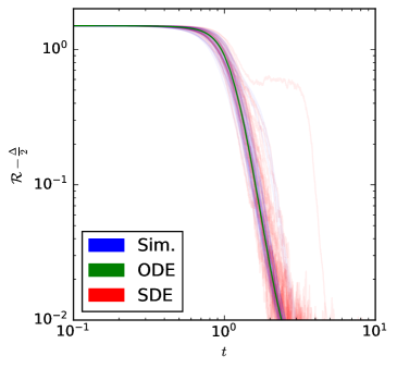
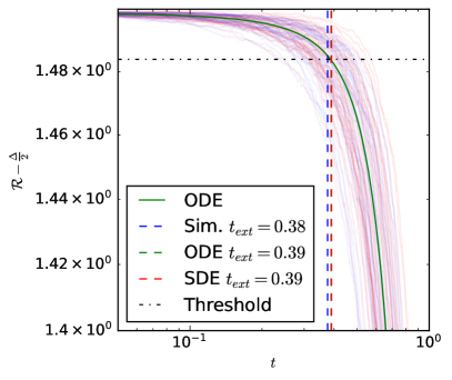
Figure 5: multiple run of the simulated SGD and the numerically integrated SDE, always starting from the same initial condition, with $d=3000$. All the $t_{\text{ext}}$ presented are obtained by solving numerically (21). The SDE captures the variance that the ODE doesn’t exhibit, but the $t_{\text{ext}}$ do not change considerably.

Appendix F Landscape geometry

In this appendix we discuss the landscape of the population risk for the phase retrieval problem $p=1$. We start by discussing the Euclidean case first, moving to the sphere next.

We recall the reader that the loss function is given by given by:

$$\ell(w)\coloneqq\ell(y,f_{\Theta}(x))=\frac{1}{2}\left((w_{\star}^{\top}x)^{2}+\sqrt{\Delta}z-(w^{\top}x)^{2}\right)^{2}$$ (63)

As before, we define the pre-activations (or local fields):

$$\lambda_{\star}=w_{\star}^{\top}x, \lambda=w^{\top}x$$ (64)

and the displacement vector:

$$\mathcal{E}(w) \coloneqq(w_{\star}^{\top}x)^{2}+\sqrt{\Delta}z-(w^{\top}x)^{2}$$

$$=\lambda_{\star}^{2}+\sqrt{\Delta}z-\lambda^{2}$$ (65)

Note that:

$$\nabla_{w}\mathcal{E}(w)=-2\lambda x$$ (66)

Therefore, the Euclidean gradient of the loss is given by:

$$\nabla_{w}\ell(w)=-2\mathcal{E}(w)\lambda x$$ (67)

And the Euclidean Hessian is:

$$\nabla^{2}\ell(w) =2\left(2\lambda^{2}-\mathcal{E}(w)\right)xx^{\top}$$

$$=2(3\lambda^{2}-\lambda_{\star}^{2}+\sqrt{\Delta}z)xx^{\top}$$ (68)

Averaged geometry —

We now compute the expected geometry by taking population averages of the above. It will be useful to define the correlation variables:

$$\rho=\frac{||w_{\star}||^{2}}{d}, m=\frac{w_{\star}^{\top}w}{d}, q=\frac{||w||^{2}}{d}$$ (69)

which we recall are the second moments of the pre-activations $(\lambda_{\star},\lambda)$. With this notation, the population risk (the expected value of (63)) reads:

$$\mathcal{R}(m,q)=\nicefrac{{\Delta}}{{2}}+3\rho^{2}+3q^{2}-4m^{2}-2\rho q$$ (70)

In order to compute the expected gradient, we need the following moments:

$$\mathbb{E}[\lambda_{\star}^{2}\lambda x]=\rho\theta+2mw_{\star}, \mathbb{E}[\lambda_{\star}^{3}x]=3qw$$ (71)

Which gives:

$$\nabla_{w}\mathcal{R}(w)=-2\mathbb{E}\left[\mathcal{E}(w)\lambda x\right]=-2((\rho-3q)w+2mw_{\star})$$ (72)

Finally, let’s compute the expected Hessian. For that, we will need the following moments:

$$\mathbb{E}[\lambda^{2}_{\star}xx^{\top}]=\rho I_{d}+w_{\star}w_{\star}^{\top}, \mathbb{E}[\lambda^{2}xx^{\top}]=qI_{d}+ww^{\top}$$ (73)

Therefore:

$$\nabla_{w}^{2}\mathcal{R}(w)=2\mathbb{E}\left[(3\lambda^{2}-\lambda_{\star}^{2}+\sqrt{\Delta}z)xx^{\top}\right]=2\left(-(\rho-3q)I_{d}+3ww^{\top}-w_{\star}w_{\star}^{\top}\right)$$ (74)

We are now ready to compute the critical points of the Euclidean landscape and evaluate their nature. By definition, the critical points are defined as solutions of $\nabla_{w}\mathcal{R}(w)=0$. These are:

• $w=0$ ($(m,q)=(0,0)$): The Hessian of this critical point is given by:

  $$\nabla_{w}^{2}\mathcal{R}(0)=-2(\rho I_{d}+w_{\star}w_{\star}^{\top})\prec 0$$ (75)

  This is a negative-definite matrix with $d-1$ negative eigenvalues $-2\rho$ and one negative eigenvalue $-2(\rho+1)$ with eigenvector $\theta_{\star}$. Therefore, this is a local maximum. The risk associated is given by:

  $$\mathcal{R}(0)=\frac{\Delta}{2}+3\rho^{2}$$ (76)

• $(m,q)=(0,\nicefrac{{\rho}}{{3}})$: This defines a line of critical points $\{w\in\mathbb{R}^{d}\mathrel{\mathop{\mathchar 58\relax}}w\perp w_{\star}\text{ and }||w||=\nicefrac{{1}}{{\sqrt{3}}}||w_{\star}||\}$. The Hessian is given by:

  $$\nabla_{w}^{2}\mathcal{R}=2(3ww^{\top}-w_{\star}w_{\star}^{\top})$$ (77)

  Note this is a rank-two matrix with $d-2$ zero eigenvalues (associated to flat directions), one negative eigenvalue with eigenvector $w_{\star}$ and a positive eigenvalue with eigenvector perpendicular to the minima. This is a saddle-point, and have population risk:

  $$\mathcal{R}(0,\nicefrac{{\rho}}{{3}})=\frac{\Delta}{2}+\frac{10}{3}\rho^{2}$$ (78)

• $w=\pm w_{\star}$ ($(m,q)=(\pm\rho,\rho)$): From the definition of our problem, this is the global minima. The expected Hessian is given by:

  $$\nabla_{w}^{2}\mathcal{R}(\pm w_{\star})=4(\rho I_{d}+w_{\star}w_{\star}^{\top})\succ 0$$ (79)

  which is indeed a positive definite matrix. This defines the minimum achievable population risk:

  $$\underset{w\in\mathbb{R}^{d}}{\min}~{}\mathcal{R}(w)=\mathcal{R}(\pm\rho,\rho)=\frac{\Delta}{2}$$ (80)

This is consistent with the discussion in [41], where the critical points and their nature were reported, but explicit expressions for the expected gradient and Hessian were not given. From this geometry, a neat picture for the one-pass SGD dynamics in the unconstrained problem can be drawn. Consider $w_{\star}\in\mathbb{S}^{d-1}$ with a random initialization at high-dimensions:

$$w^{0}\sim\mathcal{N}(0,I_{d}).$$ (81)

Note that with high-probability the random initial weights is almost orthogonal to the signal, and we have $(m,q)\approx(0,1)$. Note this is not a critical point, and the initial gradient $\nabla_{w}\mathcal{R}(w^{0})=4w^{0}$ is orthogonal to $w_{\star}$. Indeed, for $p=1$ and $\Delta=0$ the unconstrained ODEs (11) are given by:

$$\dot{m}(t) =6~{}m(t)(\rho-q(t))$$ (82)

$$\dot{q}(t) =4\left(q(t)(\rho-3q(t))+2m(t)^{2}\right)$$

$$\quad+12\gamma\left(q(t)(\rho^{2}+5q(t)^{2}-2\rho q(t))+4m^{2}(\rho-2q(t))\right)$$ (83)

where $\dot{}\coloneqq\nicefrac{{\text{d}}}{{\text{d}t}}$ and we dropped the bars for clarity. Therefore, in the initial stage of the dynamics $\dot{m}\approx 0$ remains almost constant, while $q$ decreases, and the dynamics flow in the direction of the saddle-point $(0,\nicefrac{{\rho}}{{3}})$. As we have seen, the saddle is mostly flat, with a single negative curvature direction pointing towards $w_{\star}$. This is precisely the mediocrity stage, where the dynamics slows down and SGD gets stuck for a long time before being able to develop significant correlation with $w_{\star}$ and escape.

F.1 Landscape in the sphere

Recall that the orthogonal projector on a vector $u\in\mathbb{S}^{d-1}$ is given by:

$${\rm Proj}_{u}=I_{d}-uu^{\top}$$ (84)

Therefore, the gradient on the sphere is given by:

$${\rm grad}_{\mathbb{S}^{d-1}}\ell(w) ={\rm Proj}_{\mathbb{S}^{d-1}}(\nabla_{w}\ell(w))=(I_{d}-ww^{\top})\nabla_{w}\ell(w)$$

$$=-2\mathcal{E}(w)\lambda(x-\lambda w)$$ (85)

Similarly, the Hessian on the sphere can be written as:

$${\rm Hess}_{\mathcal{S}^{d-1}}\ell(w) ={\rm Proj}_{\mathbb{S}^{d-1}}\left(\nabla_{w}^{2}\ell(w)\right)-\langle w,\nabla_{w}\ell(w)\rangle I_{d}$$

$$=(3\lambda^{2}-\lambda_{\star}^{2})(xx^{\top}-\lambda\theta x^{\top})+\mathcal{E}(w)\lambda^{2}I_{d}$$ (86)

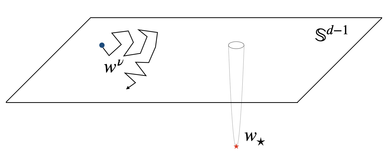
Figure 6: Low-dimensional illustration of mediocrity at initialization. As discussed in Sec. F.1, the expected Hessian at initialization is a strict saddle-point with $d-1$ flat directions and a single negative direction pointing towards the global minimum. This scenario is particularly hard for descent based algorithms such as SGD, that require $n=d\log{d}$ samples / steps to develop significant correlation with the signal.

Averaged geometry —

Recall that in the sphere we have $\rho=q=1$. Therefore, the population risk now only depends on the correlation $m=\langle w_{\star},w\rangle$, and reads:

$$\mathcal{R}(w)=2(1-m^{2})+\frac{\Delta}{2}$$ (87)

Luckily, half of the moments we need have been already computed above. To get the gradient on the sphere, we just need to compute:

$$\mathbb{E}[\lambda_{\star}^{2}\lambda^{2}]=1+2m^{2}, \mathbb{E}[\lambda^{4}]=3$$ (88)

Therefore, the averaged spherical gradient is given by:

$${\rm grad}_{\mathbb{S}^{d-1}}\mathcal{R}(w)=4m\left(mw-w_{\star}\right)$$ (89)

We also have all moments required to compute the expected spherical Hessian:

$${\rm Hess}_{\mathcal{S}^{d-1}}\mathcal{R}(w)=4\left[m^{2}I_{d}+mww_{\star}^{\top}-w_{\star}w_{\star}^{\top}\right]$$ (90)

As before, we can now analyze the critical points and their nature.

• $w\perp w_{\star}$ ($m=0$): The Hessian is given by:

  $${\rm Hess}_{\mathcal{S}^{d-1}}\mathcal{R}(w)=-4w_{\star}w_{\star}^{\top}$$ (91)

  Which is a rank one matrix with $d-1$ eigenvalues $0$ (flat directions) and a single negative eigenvalue $-4$ with negative curvature pointing towards the signal $w_{\star}$. Therefore, this is a strict saddle-point. However, since the risk is a decreasing function of $m^{2}\in[0,1]$, this is also the global maximum of the risk.

• $w=\pm w_{\star}$ ($m=\pm 1$): As before, these are the global minima, and define the minimal achievable risk $\mathcal{R}(\pm w_{\star})=\nicefrac{{\Delta}}{{2}}$. Indeed, the Hessian is given by:

  $${\rm Hess}_{\mathcal{S}^{d-1}}\mathcal{R}(\pm w_{\star})=4I_{d}\succ 0$$ (92)

  which is positive-define.

Therefore, the landscape now resembles a golf course: completely flat with a single whole corresponding with the global minimum $w_{\star}$, see Fig. 6 for an illustration. This is the prototypical image of mediocrity. In particular, differently from the unconstrained case, random initialization

$$w^{0}\sim{\rm Unif}(\mathbb{S}^{d-1}(\sqrt{d}))$$ (93)

now corresponds to initializing close to the saddle-point point $m^{0}=0$: with high-probability the initial weights are orthogonal to the signal at high-dimensions:

$$m^{0}=\nicefrac{{1}}{{d}}\langle w^{0},w_{\star}\rangle\approx\nicefrac{{1}}{{\sqrt{d}}}\ll 1.$$ (94)

For the reader convenience, we recall that the ODEs (19) describing the evolution of the correlation $m$ is given by:

$$\dot{m}(t) =m{(t)}\left[4(1-6\gamma)(1-m^{2}{(t)})-2\gamma\Delta\right]$$ (95)

Close to initialization we now have $\dot{m}(0)\approx 0$, slowing down the dynamics close to initialization.

References

- [1] Yan Shuo Tan and Roman Vershynin. Online stochastic gradient descent with arbitrary initialization solves non-smooth, non-convex phase retrieval. Journal of Machine Learning Research, 24(58):1–47, 2023.
- [2] Gerard Ben Arous, Reza Gheissari, and Aukosh Jagannath. Online stochastic gradient descent on non-convex losses from high-dimensional inference. Journal of Machine Learning Research, 22(106):1–51, 2021.
- [3] Alberto Bietti, Joan Bruna, Clayton Sanford, and Min Jae Song. Learning single-index models with shallow neural networks. In S. Koyejo, S. Mohamed, A. Agarwal, D. Belgrave, K. Cho, and A. Oh, editors, Advances in Neural Information Processing Systems, volume 35, pages 9768–9783. Curran Associates, Inc., 2022.
- [4] Alexandru Damian, Jason Lee, and Mahdi Soltanolkotabi. Neural networks can learn representations with gradient descent. In Po-Ling Loh and Maxim Raginsky, editors, Proceedings of Thirty Fifth Conference on Learning Theory, volume 178 of Proceedings of Machine Learning Research, pages 5413–5452. PMLR, 02–05 Jul 2022.
- [5] Raphaël Berthier, Andrea Montanari, and Kangjie Zhou. Learning time-scales in two-layers neural networks, 2023.
- [6] Jean Barbier, Florent Krzakala, Nicolas Macris, Léo Miolane, and Lenka Zdeborová. Optimal errors and phase transitions in high-dimensional generalized linear models. Proceedings of the National Academy of Sciences, 116(12):5451–5460, 2019.
- [7] Antoine Maillard, Bruno Loureiro, Florent Krzakala, and Lenka Zdeborová. Phase retrieval in high dimensions: Statistical and computational phase transitions. In H. Larochelle, M. Ranzato, R. Hadsell, M.F. Balcan, and H. Lin, editors, Advances in Neural Information Processing Systems, volume 33, pages 11071–11082. Curran Associates, Inc., 2020.
- [8] Song Mei, Theodor Misiakiewicz, and Andrea Montanari. Generalization error of random feature and kernel methods: Hypercontractivity and kernel matrix concentration. Applied and Computational Harmonic Analysis, 59:3–84, 2022. Special Issue on Harmonic Analysis and Machine Learning.
- [9] Stefano Sarao Mannelli, Eric Vanden-Eijnden, and Lenka Zdeborová. Optimization and generalization of shallow neural networks with quadratic activation functions. In H. Larochelle, M. Ranzato, R. Hadsell, M.F. Balcan, and H. Lin, editors, Advances in Neural Information Processing Systems, volume 33, pages 13445–13455. Curran Associates, Inc., 2020.
- [10] David Saad and Sara A. Solla. Exact solution for on-line learning in multilayer neural networks. Phys. Rev. Lett., 74:4337–4340, May 1995.
- [11] David Saad and Sara A. Solla. On-line learning in soft committee machines. Phys. Rev. E, 52:4225–4243, Oct 1995.
- [12] David Saad and Sara Solla. Dynamics of on-line gradient descent learning for multilayer neural networks. In D. Touretzky, M. C. Mozer, and M. Hasselmo, editors, Advances in Neural Information Processing Systems, volume 8. MIT Press, 1996.
- [13] P Riegler and M Biehl. On-line backpropagation in two-layered neural networks. Journal of Physics A: Mathematical and General, 28(20):L507–L513, oct 1995.
- [14] M Copelli and N Caticha. On-line learning in the committee machine. Journal of Physics A: Mathematical and General, 28(6):1615–1625, mar 1995.
- [15] G. Reents and R. Urbanczik. Self-averaging and on-line learning. Phys. Rev. Lett., 80:5445–5448, Jun 1998.
- [16] Sebastian Goldt, Madhu Advani, Andrew M Saxe, Florent Krzakala, and Lenka Zdeborová. Dynamics of stochastic gradient descent for two-layer neural networks in the teacher-student setup. Advances in neural information processing systems, 32, 2019.
- [17] Sebastian Goldt, Marc Mézard, Florent Krzakala, and Lenka Zdeborová. Modeling the influence of data structure on learning in neural networks: The hidden manifold model. Phys. Rev. X, 10:041044, Dec 2020.
- [18] Sebastian Goldt, Bruno Loureiro, Galen Reeves, Florent Krzakala, Marc Mézard, and Lenka Zdeborová. The gaussian equivalence of generative models for learning with two-layer neural networks. In Proceedings of Machine Learning Research, volume 145, pages 1–46. 2nd Annual Conference on Mathematical and Scientific Machine Learning, 2021.
- [19] Rodrigo Veiga, Ludovic Stephan, Bruno Loureiro, Florent Krzakala, and Lenka Zdeborova. Phase diagram of stochastic gradient descent in high-dimensional two-layer neural networks. In Alice H. Oh, Alekh Agarwal, Danielle Belgrave, and Kyunghyun Cho, editors, Advances in Neural Information Processing Systems, 2022.
- [20] Luca Arnaboldi, Ludovic Stephan, Florent Krzakala, and Bruno Loureiro. From high-dimensional & mean-field dynamics to dimensionless odes: A unifying approach to sgd in two-layers networks, 2023.
- [21] Gerard Ben Arous, Reza Gheissari, and Aukosh Jagannath. High-dimensional limit theorems for sgd: Effective dynamics and critical scaling. Advances in Neural Information Processing Systems, 35:25349–25362, 2022.
- [22] Song Mei, Andrea Montanari, and Phan-Minh Nguyen. A mean field view of the landscape of two-layer neural networks. Proceedings of the National Academy of Sciences, 115(33):E7665–E7671, 2018.
- [23] Lenaic Chizat and Francis Bach. On the global convergence of gradient descent for over-parameterized models using optimal transport. Advances in neural information processing systems, 31, 2018.
- [24] Grant Rotskoff and Eric Vanden-Eijnden. Trainability and accuracy of artificial neural networks: An interacting particle system approach. Communications on Pure and Applied Mathematics, 75(9):1889–1935, 2022.
- [25] Behrooz Ghorbani, Song Mei, Theodor Misiakiewicz, and Andrea Montanari. Limitations of lazy training of two-layers neural network. In H. Wallach, H. Larochelle, A. Beygelzimer, F. d'Alché-Buc, E. Fox, and R. Garnett, editors, Advances in Neural Information Processing Systems, volume 32. Curran Associates, Inc., 2019.
- [26] Justin Sirignano and Konstantinos Spiliopoulos. Mean field analysis of neural networks: A central limit theorem. Stochastic Processes and their Applications, 130(3):1820–1852, 2020.
- [27] Emmanuel Abbe, Enric Boix Adsera, and Theodor Misiakiewicz. The merged-staircase property: a necessary and nearly sufficient condition for sgd learning of sparse functions on two-layer neural networks. In Conference on Learning Theory, pages 4782–4887. PMLR, 2022.
- [28] Emmanuel Abbe, Enric Boix-Adsera, and Theodor Misiakiewicz. Sgd learning on neural networks: leap complexity and saddle-to-saddle dynamics, 2023.
- [29] Karl Hajjar and Lénaν̈c Chizat. On the symmetries in the dynamics of wide two-layer neural networks. Electronic Research Archive, 31(4):2175–2212, 2023.
- [30] Arthur Jacot, François Ged, Berfin Şimşek, Clément Hongler, and Franck Gabriel. Saddle-to-saddle dynamics in deep linear networks: Small initialization training, symmetry, and sparsity, 2022.
- [31] Etienne Boursier, Loucas Pillaud-Vivien, and Nicolas Flammarion. Gradient flow dynamics of shallow relu networks for square loss and orthogonal inputs. In S. Koyejo, S. Mohamed, A. Agarwal, D. Belgrave, K. Cho, and A. Oh, editors, Advances in Neural Information Processing Systems, volume 35, pages 20105–20118. Curran Associates, Inc., 2022.
- [32] Kishore Jaganathan, Yonina C. Eldar, and Babak Hassibi. Phase Retrieval: An Overview of Recent Developments. CRC Press, 2016.
- [33] Jonathan Dong, Lorenzo Valzania, Antoine Maillard, Thanh-an Pham, Sylvain Gigan, and Michael Unser. Phase retrieval: From computational imaging to machine learning: A tutorial. IEEE Signal Processing Magazine, 40(1):45–57, 2023.
- [34] Emmanuel J. Candès, Yonina C. Eldar, Thomas Strohmer, and Vladislav Voroninski. Phase retrieval via matrix completion. SIAM Journal on Imaging Sciences, 6(1):199–225, 2013.
- [35] Emmanuel J. Candès, Thomas Strohmer, and Vladislav Voroninski. Phaselift: Exact and stable signal recovery from magnitude measurements via convex programming. Communications on Pure and Applied Mathematics, 66(8):1241–1274, 2013.
- [36] Emmanuel J. Candès, Xiaodong Li, and Mahdi Soltanolkotabi. Phase retrieval via wirtinger flow: Theory and algorithms. IEEE Transactions on Information Theory, 61(4):1985–2007, 2015.
- [37] Marco Mondelli and Andrea Montanari. Fundamental limits of weak recovery with applications to phase retrieval. In Sébastien Bubeck, Vianney Perchet, and Philippe Rigollet, editors, Proceedings of the 31st Conference On Learning Theory, volume 75 of Proceedings of Machine Learning Research, pages 1445–1450. PMLR, 06–09 Jul 2018.
- [38] Benjamin Aubin, Bruno Loureiro, Antoine Baker, Florent Krzakala, and Lenka Zdeborová. Exact asymptotics for phase retrieval and compressed sensing with random generative priors. In Jianfeng Lu and Rachel Ward, editors, Proceedings of The First Mathematical and Scientific Machine Learning Conference, volume 107 of Proceedings of Machine Learning Research, pages 55–73. PMLR, 20–24 Jul 2020.
- [39] Ju Sun, Qing Qu, and John Wright. A geometric analysis of phase retrieval. In 2016 IEEE International Symposium on Information Theory (ISIT), pages 2379–2383, 2016.
- [40] Yan Shuo Tan and Roman Vershynin. Phase retrieval via randomized Kaczmarz: theoretical guarantees. Information and Inference: A Journal of the IMA, 8(1):97–123, 04 2018.
- [41] Yuxin Chen, Yuejie Chi, Jianqing Fan, and Cong Ma. Gradient descent with random initialization: fast global convergence for nonconvex phase retrieval. Mathematical Programming, 176(1):5–37, Jul 2019.
- [42] Damek Davis, Dmitriy Drusvyatskiy, and Courtney Paquette. The nonsmooth landscape of phase retrieval. IMA Journal of Numerical Analysis, 40(4):2652–2695, 01 2020.
- [43] Stefano Sarao Mannelli, Giulio Biroli, Chiara Cammarota, Florent Krzakala, Pierfrancesco Urbani, and Lenka Zdeborová. Complex dynamics in simple neural networks: Understanding gradient flow in phase retrieval. In H. Larochelle, M. Ranzato, R. Hadsell, M.F. Balcan, and H. Lin, editors, Advances in Neural Information Processing Systems, volume 33, pages 3265–3274. Curran Associates, Inc., 2020.
- [44] Francesca Mignacco, Pierfrancesco Urbani, and Lenka Zdeborová. Stochasticity helps to navigate rough landscapes: comparing gradient-descent-based algorithms in the phase retrieval problem. Machine Learning: Science and Technology, 2(3):035029, jul 2021.
- [45] Herbert Robbins and Sutton Monro. A Stochastic Approximation Method. The Annals of Mathematical Statistics, 22(3):400 – 407, 1951.
- [46] Georg Ch. Pflug. Stochastic minimization with constant step-size: Asymptotic laws. SIAM Journal on Control and Optimization, 24(4):655–666, 1986.
- [47] Aymeric Dieuleveut, Alain Durmus, and Francis Bach. Bridging the gap between constant step size stochastic gradient descent and Markov chains. The Annals of Statistics, 48(3):1348 – 1382, 2020.
- [48] Francis Bach and Lénaic Chizat. Gradient descent on infinitely wide neural networks: Global convergence and generalization. In International Congress of Mathematicians, 2022.
- [49] Caibin Zeng. Mean exit time and escape probability for the ornstein–uhlenbeck process. Chaos: An Interdisciplinary Journal of Nonlinear Science, 30(9):093127, 2020.