A Bayesian sparse factor model with adaptive posterior concentrationThis work was supported by the National Research Foundation of Korea (NRF) grant funded by the Korea government (MSIT) (No. 2020R1A2C3A01003550 and No. 2022R1F1A1069695). Lizhen Lin would like to acknowledge the generous support of NSF grants DMS CAREER 1654579 and DMS 2113642.

Abstract

In this paper, we propose a new Bayesian inference method for a high-dimensional sparse factor model that allows both the factor dimensionality and the sparse structure of the loading matrix to be inferred. The novelty is to introduce a certain dependence between the sparsity level and the factor dimensionality, which leads to adaptive posterior concentration while keeping computational tractability. We show that the posterior distribution asymptotically concentrates on the true factor dimensionality, and more importantly, this posterior consistency is adaptive to the sparsity level of the true loading matrix and the noise variance. We also prove that the proposed Bayesian model attains the optimal detection rate of the factor dimensionality in a more general situation than those found in the literature. Moreover, we obtain a near-optimal posterior concentration rate of the covariance matrix. Numerical studies are conducted and show the superiority of the proposed method compared with other competitors.

SReferences

, and

1 Introduction

In this paper, we propose a novel Bayesian method for learning a high-dimensional sparse linear factor model and study asymptotic concentration properties of the posterior distribution. We consider the following linear factor model where $p$-dimensional random vectors $\mathbf{Y}_{1},\dots,\mathbf{Y}_{n}$ are distributed as

$$\mathbf{Y}_{i}|(\mathbf{Z}_{i}=\mathbf{z}_{i})\stackrel{{\scriptstyle\textup{ind}}}{{\sim}}\texttt{{N}}(\mathbf{B}\mathbf{z}_{i},\psi\mathbf{I}),\quad\mathbf{Z}_{i}\stackrel{{\scriptstyle\textup{iid}}}{{\sim}}\texttt{{N}}(\mathbf{0},\mathbf{I})$$ (1.1)

for $i\in[n]$ with $\mathbf{B}$ representing a $p\times\xi$ factor loading matrix, $\psi>0$ a noise variance and $\mathbf{Z}_{i}$ a $\xi$-dimensional (latent) factor related to datum $\mathbf{Y}_{i}$, where $\xi\in\{1,\dots,p-1\}$. Under this model, the marginal distribution of the data $\mathbf{Y}_{1},\dots,\mathbf{Y}_{n}$ is given by

$$\mathbf{Y}_{i}\stackrel{{\scriptstyle\textup{iid}}}{{\sim}}\texttt{{N}}(\mathbf{0},\bm{\Sigma}),\quad\bm{\Sigma}\mathrel{\mathop{\mathchar 58\relax}}=\mathbf{B}\mathbf{B}^{\top}+\psi\mathbf{I}.$$

Therefore, correlations among the observed variables in each $\mathbf{Y}_{i}$ in the above factor model are explained by a low rank matrix $\mathbf{B}\mathbf{B}^{\top}$ which leads to a substantial but efficient reduction of the model complexity. The factor model has been used in a broad range of high-dimensional inference tasks including covariance estimation (Fan et al., 2008, 2011, 2018b), linear regression (Bai and Ng, 2006; Kneip and Sarda, 2011; Stock and Watson, 2002), multiple testing under arbitrary dependence (Fan et al., 2012, 2018a; Leek and Storey, 2008) and other supervised learning tasks (Fan et al., 2017; Silva, 2011).

For high-dimensional data where the dimension $p$ is much large than the sample size $n,$ we need a low dimensional structure on $\mathbf{B}$ to have a consistent estimator and sparsity is a popularly used condition, which assumes that true loading matrix $\mathbf{B}^{\star}$ is sparse in the sense that only few entries of $\mathbf{B}^{\star}$ is nonzero and the other entries are zero. There are various Bayesian models for sparse linear factor models including Bhattacharya and Dunson (2011); Srivastava et al. (2017); Xie et al. (2022); Ning (2021).

Along with considering the sparsity, determining the factor dimensionality $\xi$ is an important and practical topic in factor modeling. From a theoretical point of view, an appropriate estimation of the factor dimensionality is required to optimize the bias-variance trade-off in a factor model. The factor dimensionality is also of practical interest, especially when it has a physical interpretation e.g., the number of interacting pathways in genomics (Carvalho et al., 2008) and the number of personality traits in psychology (Caprara et al., 1993).

Frequentist approaches typically adopt a two-step procedure where the factor dimensionality is chosen or estimated before estimating the parameters in the model. Many consistent model selection methods have been proposed, which fit the factor models for different values of $\xi$ and select the best $\xi$ based on their choice of model selection criteria (Bai and Ng, 2002, 2007). Alternatively, the eigenvalues of the empirical covariance or correlation matrix can be used to estimate the factor dimensionality. Several procedures related to this approach have been proposed and yielded consistency (Ahn and Horenstein, 2013; Fan et al., 2020; Lam and Yao, 2012; Onatski, 2010). The estimation of the factor dimensionality for high-dimensional sparse factor models has also been considered by Cai et al. (2013, 2015).

On the Bayesian side, prior distributions which put prior mass on $\xi$ directly have been popularly used to infer the factor dimensionality. Examples are the spike and slab prior with the Poisson prior on $\xi$ (Pati et al., 2014) and spike and slap priors with the Indian buffet process (IBP) (Chen et al., 2010; Knowles and Ghahramani, 2011; Rockova and George, 2016; Ohn and Kim, 2022). Recently, a few works have provided theoretical results for the posterior distribution of the factor dimensionality under nonparametric priors. Rockova and George (2016) considered a spike and slab prior with the one-parameter IBP and proved that the posterior probability of the factor dimensionality being upper bounded by a certain quantity converges to 1. But the upper bound is much larger than the true factor dimensionality. Ohn and Kim (2022) derived posterior consistency of the factor dimensionality under a spike and slab prior with the two-parameter IBP. However, their result is nonadaptive in the sense that the choice of hyperparameters of the prior distribution relies on the information or knowledge of the true sparsity of the loading matrix, which is unknown in practice.

Another promising theoretical result was provided by Gao and Zhou (2015). The authors studied the Bayesian factor model in the context of sparse principle component analysis (PCA) in which the prior distribution concentrates its mass on the orthogonal loading matrix, i.e., $\mathbf{B}^{\top}\mathbf{B}$ is diagonal, and established the adaptive posterior consistency of the factor dimensionality. However, the orthogonal constraint makes it hard to compute posterior distribution and Gao and Zhou (2015) only succeeded in implementing a posterior sampler for the factor model with a one-dimensional factor i.e., $\xi=1$.

We propose a novel Bayesian model that overcomes the theoretical and practical limitations of the existing Bayesian approaches. A key feature of the proposed Bayesian model is that the sparsity and the factor dimensionality are negatively correlated under the prior distribution, and this a priori negative correlation between them helps to prevent overestimating the true factor dimensionality. This is a critical difference between the proposed prior and the widely used IBP-type priors. Yet, posterior computation can be carried out through a simple and efficient Monte Carlo Markov chain (MCMC) algorithm. Our numerical studies show that the developed MCMC algorithm can apply to high-dimensional data without many hampers.

We thoroughly investigate the theoretical properties of the posterior distribution of the proposed Bayesian model. We prove that the posterior distribution of the factor dimensionality converges to the true one. In particular, we prove that the proposed Bayesian model attains the optimal detection rate for the eigengap (i.e., the size of the smallest eigenvalue of the low rank part $\mathbf{B}^{\star}(\mathbf{B}^{\star})^{\top}$ of the true covariance matrix $\bm{\Sigma}^{\star}=\mathbf{B}^{\star}(\mathbf{B}^{\star})^{\top}+\psi^{\star}\mathbf{I}$) for the consistency of the factor dimensionality. We also show that the posterior distribution of the covariance matrix concentrates around the truth at a near optimal rate. The novelty of our results lies in that it does not require any prior knowledge of the true sparsity and noise variance and hence all the optimal theoretical properties of the posterior are adaptive to the sparsity and noise variance.

It should be noted that the proposed Bayesian model has theoretical advantages over not only other Bayesian factor models but also existing frequentist’s estimators of the factor dimensionality. The estimator of Cai et al. (2013) is adaptive to the true sparsity but requires a larger detection rate for the eigengap than the optimal one. On the other hand, the estimator of Cai et al. (2015) achieves the optimal detection rate but is not adaptive to the true sparsity. Moreover, both estimators assume the known noise variance, which limits their applicability.

The rest of the paper is organized as follows. In Section 2, we introduce the proposed prior distribution and develop an efficient MCMC algorithm for sampling from the posterior distribution. In Section 3, asymptotic properties of the posterior distribution are derived. In Section 4, we conduct simulation studies and real data analysis. Section 5 concludes the paper.

1.1 Notation

Let $\mathbb{R}$, $\mathbb{R}_{+}$ and $\mathbbm{N}$ be the sets of real numbers, positive numbers and natural numbers, respectively. Let $\mathbf{0}$ and $\mathbf{1}$ denote vectors of 0’s and of 1’s, respectively, where the dimensions of such vectors can differ according to the context. For a positive integer $p$, we let $[p]\mathrel{\mathop{\mathchar 58\relax}}=\{1,2,\dots,p\}$. For a real number $x$, $\left\lfloor{x}\right\rfloor$ denote the largest integer less than or equal to $x$ and $\left\lceil{x}\right\rceil$ denote the smallest integer larger than or equal to $x$. For two real numbers $a$ and $b$, we write $a\vee b\mathrel{\mathop{\mathchar 58\relax}}=\max\{a,b\}$ and $a\wedge b\mathrel{\mathop{\mathchar 58\relax}}=\min\{a,b\}$. For two positive sequences $\{a_{n}\}_{n\in\mathbb{N}}$ and $\{b_{n}\}_{n\in\mathbb{N}}$ we write $a_{n}\lesssim b_{n}$ or equivalently $b_{n}\gtrsim a_{n}$ if there exists a positive constant $C>0$ such that $a_{n}\leq Cb_{n}$ for any $n\in\mathbb{N}$. Moreover, we write $a_{n}\asymp b_{n}$ if both $a_{n}\lesssim b_{n}$ and $a_{n}\gtrsim b_{n}$ hold. We denote by $\mathbbm{1}(\cdot)$ the indicator function.

For a set $\mathcal{S}$, $|\mathcal{S}|$ denotes its cardinality. For a $p$-dimensional vector $\bm{\beta}\mathrel{\mathop{\mathchar 58\relax}}=(\beta_{j})_{j\in[p]}$, let $\|\bm{\beta}\|_{r}\mathrel{\mathop{\mathchar 58\relax}}=\mathinner{(\sum_{j=1}^{p}|\beta_{j}|^{r})}^{1/r}$ for $r\geq 1$ and $\|\bm{\beta}\|_{0}\mathrel{\mathop{\mathchar 58\relax}}=\sum_{j=1}^{p}\mathbbm{1}(\beta_{j}\neq 0)$. For a set $\mathcal{S}\subset\{1,\dots,p\}$, define $\bm{\beta}_{[\mathcal{S}]}\mathrel{\mathop{\mathchar 58\relax}}=(\beta_{j})_{j\in\mathcal{S}}$. For a $p\times q$-dimensional matrix $\mathbf{A}\mathrel{\mathop{\mathchar 58\relax}}=(a_{jk})_{j\in[p],k\in[q]}$, we denote the spectral norm of the matrix $\mathbf{A}$ by $\mathinner{\!\left\lVert\mathbf{A}\right\rVert}$ and the Frobenius norm by $\left\|{\mathbf{A}}\right\|_{\textup{F}}$, that is, $\mathinner{\!\left\lVert\mathbf{A}\right\rVert}\mathrel{\mathop{\mathchar 58\relax}}=\sup_{\mathbf{x}\in\mathbb{R}^{q}\mathrel{\mathop{\mathchar 58\relax}}\|\mathbf{x}\|_{2}=1}\|\mathbf{A}\mathbf{x}\|_{2}$ and $\left\|{\mathbf{A}}\right\|_{\textup{F}}\mathrel{\mathop{\mathchar 58\relax}}=\sqrt{\textup{Tr}(\mathbf{A}^{\top}\mathbf{A})}$. Let $\mathinner{\!\left\lVert\mathbf{A}\right\rVert}_{1}$ be the vector $\ell_{1}$ norm of $\mathbf{A}$, i.e., $\mathinner{\!\left\lVert\mathbf{A}\right\rVert}_{1}\mathrel{\mathop{\mathchar 58\relax}}=\sum_{j=1}^{p}\sum_{k=1}^{q}|a_{jk}|$. For sets $\mathcal{S}\subset[p]$ and $\mathcal{K}\subset[q]$, we let $\mathbf{A}_{[\mathcal{S},\mathcal{K}]}\mathrel{\mathop{\mathchar 58\relax}}=(a_{jk})_{j\in\mathcal{S},k\in\mathcal{K}}$ which is the submatrix of $\mathbf{A}$ taking the rows in $\mathcal{S}$ and columns in $\mathcal{K}$. For notational simplicity, we write $\mathbf{A}_{[\mathrel{\mathop{\mathchar 58\relax}},\mathcal{K}]}\mathrel{\mathop{\mathchar 58\relax}}=\mathbf{A}_{[[p],\mathcal{K}]}$ and $\mathbf{A}_{[\mathcal{S},\mathrel{\mathop{\mathchar 58\relax}}]}\mathrel{\mathop{\mathchar 58\relax}}=\mathbf{A}_{[\mathcal{S},[q]]}$. Furthermore, let $\mathbf{A}_{[j,\mathrel{\mathop{\mathchar 58\relax}}]}\mathrel{\mathop{\mathchar 58\relax}}=\mathbf{A}_{[\{j\},\mathrel{\mathop{\mathchar 58\relax}}]}$ and $\mathbf{A}_{[\mathrel{\mathop{\mathchar 58\relax}},k]}\mathrel{\mathop{\mathchar 58\relax}}=\mathbf{A}_{[\mathrel{\mathop{\mathchar 58\relax}},\{k\}]}$, which denote the $j$-th row and $k$-th column of $\mathbf{A}$, respectively. We let $\lambda_{1}(\bm{\Sigma})\geq\lambda_{2}(\bm{\Sigma})\dots\geq\lambda_{p}(\bm{\Sigma})$ be the ordered eigenvalues and $|\bm{\Sigma}|$ be the determinant of a $p\times p$-dimensional matrix $\bm{\Sigma}$. Let $\mathbbm{S}_{++}^{p}$ be a set of $p\times p$ symmetric positive definite matrices.

For a given probability measure $G$, let $\mathsf{P}_{G}$ denote the probability or the expectation operator under the probability measure $G$. We denote by $\mathsf{p}_{G}$ the probability density function of $G$ with respect to the Lebesgue measure if exists. For convenience, we write $\mathsf{P}_{\bm{\Sigma}}\mathrel{\mathop{\mathchar 58\relax}}=\mathsf{P}_{\texttt{{N}}(\mathbf{0},\bm{\Sigma})}$ and $\mathsf{p}_{\bm{\Sigma}}\mathrel{\mathop{\mathchar 58\relax}}=\mathsf{p}_{\texttt{{N}}(\mathbf{0},\bm{\Sigma})}$ for a normal distribution $\texttt{{N}}(\mathbf{0},\bm{\Sigma})$. For $n\in\mathbbm{N}$, let $\mathsf{P}_{G}^{(n)}$ be the probability or the expectation under the product measure and, if exists, $\mathsf{p}_{G}^{(n)}$ its density function.

2 Proposed prior and MCMC algorithm

In this section, we design a novel prior tailored for the loading matrix in a factor model and develop a computationally efficient MCMC algorithm for sampling the posterior distribution.

2.1 Prior distribution

The proposed prior on the loading matrix first samples the “sparse structure” of the loading matrix and then samples nonzero elements. Let $\mathbf{u}\mathrel{\mathop{\mathchar 58\relax}}=(u_{1},\dots,u_{p})^{\top}\in\Delta_{p}\mathrel{\mathop{\mathchar 58\relax}}=\{0,1\}^{p}\setminus\{\mathbf{0}\}$ and, for a positive integer $q\in\mathbbm{N}$ we have chosen, $\mathbf{v}\mathrel{\mathop{\mathchar 58\relax}}=(v_{1},\dots,v_{q})^{\top}\in\Delta_{q}\mathrel{\mathop{\mathchar 58\relax}}=\{0,1\}^{q}\setminus\{\mathbf{0}\}$. They are latent indicator variables that determine nonzero rows and columns of the loading matrix $\mathbf{B}$, respectively. Note that the sparsity of columns determines the factor dimensionality $\xi$, i.e., $\xi=\|\mathbf{v}\|_{0}$ and $q$ is a pre-specified upper bound of the factor dimensionality. We impose the prior distribution on $\mathbf{u}$ and $\mathbf{v}$ such that

$$\Pi(\mathbf{u},\mathbf{v})= \frac{Q_{A}(\|\mathbf{u}\|_{0},\|\mathbf{v}\|_{0})}{\sum_{\mathbf{u}^{\prime}\in\Delta_{p}}\sum_{\mathbf{v}^{\prime}\in\Delta_{q}}Q_{A}(\|\mathbf{u}^{\prime}\|_{0},\|\mathbf{v}^{\prime}\|_{0})}\mathbbm{1}(\mathbf{u}\in\Delta_{p},\mathbf{v}\in\Delta_{q})$$ (2.1)

$$\mbox{ with }Q_{A}(\omega,\xi)\mathrel{\mathop{\mathchar 58\relax}}=Q_{A,p,q,n}(\omega,\xi)\mathrel{\mathop{\mathchar 58\relax}}=\frac{1}{\binom{p}{\omega}\binom{q}{\xi}}\exp({-A\omega\xi\log(p\vee n)})$$

for some $A>0$. Under this prior distribution, the non-sparsity $\omega=\|\mathbf{u}\|_{0}$ and the factor dimensionality $\xi=\|\mathbf{v}\|_{0}$ are negatively correlated in the sense that $\omega$ becomes smaller when $\xi$ is large and vice versa. Note that $\|\mathbf{u}\|_{0}$ and $\|\mathbf{v}\|_{0}$ are negatively correlated in the proposed prior (2.1), which sharply contrasts with existing IBP-type priors (Rockova and George, 2016; Ohn and Kim, 2022) that assume the independence of $\|\mathbf{u}\|_{0}$ and $\|\mathbf{v}\|_{0}.$ The IBP-type priors, however, are known to have the posterior consistency only when the true sparsity is known. We devise the prior (2.1) to achieve an optimal posterior concentration rate even when the true sparsity is unknown.

Conditional on $\mathbf{u}$ and $\mathbf{v},$ we then impose the prior distribution of the loading matrix $\mathbf{B}$ such that

$$\Pi(\mathbf{B}\in\mathcal{B}|\mathbf{u},\mathbf{v})=\int_{\mathcal{B}}\prod_{j=1}^{p}\prod_{k=1}^{q}\mathinner{\left[\delta_{0}(\beta_{jk})\right]}^{1-u_{j}v_{k}}\mathinner{\left[\mathsf{p}_{\texttt{{Lap}}(1)}(\beta_{jk})\right]}^{u_{j}v_{k}}\textup{d}\beta_{jk}$$ (2.2)

for any measurable set $\mathcal{B}\subset\mathbb{R}^{p\times q}$, where $\delta_{0}$ denotes the Dirac-delta function at $0$ and $\texttt{{Lap}}(1)$ does the Laplace distribution with scale 1. That is, independently for each loading $\beta_{jk}$, we consider a spike and slab type prior distribution with the Dirac spike and Laplace slab. The use of the Laplace slab, which is more diffused than the normal distribution, is commonly used in Bayesian sparse factor models (Rockova and George, 2016; Xie et al., 2022; Ning, 2021; Ohn and Kim, 2022) in order to reduce bias in the estimation of large loadings.

Lastly, we consider the inverse Gamma prior distribution for $\psi$ such that

$$\Pi(\psi\in\mathcal{B}^{\prime})=\mathsf{P}_{\texttt{{IG}}(\mathbf{a})}(\psi\in\mathcal{B}^{\prime}).$$ (2.3)

for any measurable set $\mathcal{B}^{\prime}\subset\mathbb{R}$, where $\texttt{{IG}}(\mathbf{a})$ with $\mathbf{a}\mathrel{\mathop{\mathchar 58\relax}}=(a_{1},a_{2})\in\mathbb{R}_{+}^{2}$ denotes the inverse gamma distribution with shape $a_{1}$ and rate $a_{2}$.

The proposed prior is carefully designed to attain the posterior consistency of the factor dimensionality adaptively to the sparsity, therefore we call the prior defined through 2.1, 2.2 and 2.3 the adaptive spike and slab (AdaSS) prior.

2.2 Posterior computation

In this section, we develop an MCMC algorithm to compute the posterior distribution of the parameters $\mathbf{u}\mathrel{\mathop{\mathchar 58\relax}}=(u_{j})_{j\in[p]}$, $\mathbf{v}\mathrel{\mathop{\mathchar 58\relax}}=(v_{k})_{k\in[q]}$, $\mathbf{B}\mathrel{\mathop{\mathchar 58\relax}}=(\beta_{jk})_{j\in[p],k\in[q]}$, $\psi$ and the latent factors $\mathbf{Z}_{1},\dots,\mathbf{Z}_{n}$. We first introduce additional notations. Let $Y_{ij}$ be the $j$-th element of $\mathbf{Y}_{i}$ and $Z_{ik}$ be the $k$-th element of $\mathbf{Z}_{i}$. Let $\mathcal{S}\mathrel{\mathop{\mathchar 58\relax}}=\{j\in[p]\mathrel{\mathop{\mathchar 58\relax}}u_{j}=1\}$ and $\mathcal{K}\mathrel{\mathop{\mathchar 58\relax}}=\{k\in[q]\mathrel{\mathop{\mathchar 58\relax}}v_{k}=1\}$. We use the notation $f(Y|X=x)$ to denote the conditional density of $Y$ given $X=x$.

To make posterior sampling of the factor loading $\beta_{jk}$ easy, we employ the scale mixture representation of the Laplace distribution. Note that if $\beta_{jk}|\tau_{jk}\sim\texttt{{N}}(0,\tau_{jk})$ and $\tau_{jk}\sim\texttt{{Exp}}(1/2)$, then marginally we have $\beta_{jk}\sim\texttt{{Lap}}(1),$ where $\texttt{{Exp}}(1/2)$ stands for the exponential distribution with mean $2$. In the MCMC algorithm, we introduce auxiliary scale parameters $\tau_{jk}$ for $j\in[p]$ and $k\in[q]$.

Then a single iteration of our proposed MCMC sampler goes as follows.

Sample $\beta_{jk}$ for $j\in[p]$ and $k\in[q]$: We sample $\beta_{jk}$ from

$$\beta_{jk}|-\sim\begin{cases}\texttt{{N}}(\hat{\beta}_{jk},\hat{\tau}_{jk})&\mbox{if $u_{j}=1$ and $v_{k}=1$}\\ \delta_{0}&\mbox{otherwise },\end{cases}$$

where

$$\widehat{\beta}_{jk} \mathrel{\mathop{\mathchar 58\relax}}=\widehat{\tau}_{jk}\mathinner{\left\{\psi^{-1}\sum_{i=1}^{n}Z_{ik}\mathinner{\Bigl{(}Y_{ij}-\sum_{h\in[q]\mathrel{\mathop{\mathchar 58\relax}}h\neq k}Z_{ih}\beta_{jh}\Bigr{)}}\right\}}$$ (2.4)

$$\widehat{\tau}_{jk} \mathrel{\mathop{\mathchar 58\relax}}=\mathinner{\left(\psi^{-1}\sum_{i=1}^{n}Z_{ik}^{2}+\tau_{jk}^{-1}\right)}^{-1}.$$ (2.5)

Sample $\tau_{jk}$ for $j\in[p]$ and $k\in[q]$: We sample $\tau_{jk}$ from

$$\tau_{jk}|-\sim\begin{cases}\texttt{{GIG}}(1,\beta_{jk}^{2},\frac{1}{2})&\mbox{if $u_{j}=1$},\\ \texttt{{Exp}}(\frac{1}{2})&\mbox{otherwise,}\end{cases}$$ (2.6)

where $\texttt{{GIG}}(a,b,c)$ denotes the generalized inverse Gaussian distribution with density $\mathsf{p}_{\texttt{{GIG}}(a,b,c)}(z)\propto z^{c-1}\textup{e}^{-(az+b/z)/2}\mathbbm{1}(z>0).$

Sample $u_{j}$ for $j\in[p]$: If $\mathcal{S}\setminus\{j\}=\emptyset$, we set $u_{j}=1$. Otherwise, we sample $u_{j}$ from $\texttt{{Bernoulli}}(\rho_{j}^{\text{row}}/(1+\rho_{j}^{\text{row}}))$ with

$$\rho_{j}^{\text{row}} \mathrel{\mathop{\mathchar 58\relax}}=\frac{\Pi(u_{j}=1|-)}{\Pi(u_{j}=0|-)}$$ (2.7)

$$=\frac{Q_{A}(|\mathcal{S}\setminus\{j\}|+1,|\mathcal{K}|)}{Q_{A}(|\mathcal{S}\setminus\{j\}|,|\mathcal{K}|)}\frac{\prod_{i=1}^{n}f(\mathbf{Y}_{i}|u_{j}=1,\mathbf{v},\mathbf{T}_{j,\mathcal{K}},\mathbf{B}_{[-j,\mathrel{\mathop{\mathchar 58\relax}}]},\psi,\mathbf{Z}_{i})}{\prod_{i=1}^{n}f(\mathbf{Y}_{i}|u_{j}=0,\mathbf{B}_{[-j,\mathrel{\mathop{\mathchar 58\relax}}]},\psi,\mathbf{Z}_{i})}$$

$$=(p\vee n)^{-A|\mathcal{K}|}\frac{\binom{p}{|\mathcal{S}\setminus\{j\}|}}{\binom{p}{|\mathcal{S}\setminus\{j\}|+1}}\frac{\int\prod_{i=1}^{n}f(\mathbf{Y}_{i}|\mathbf{B},\psi,\mathbf{Z}_{i})\prod_{k=1}^{q}\mathinner{\left\{\mathsf{p}_{\texttt{{N}}(0,\tau_{jk})}(\beta_{jk})\right\}}^{v_{k}}\mathinner{\left\{\delta_{0}(\beta_{jk})\right\}}^{1-v_{k}}\textup{d}\beta_{jk}}{\prod_{i=1}^{n}f(\mathbf{Y}_{i}|\mathbf{B}_{[j,\mathrel{\mathop{\mathchar 58\relax}}]}=\mathbf{0},\mathbf{B}_{[-j,\mathrel{\mathop{\mathchar 58\relax}}]},\psi,\mathbf{Z}_{i})}$$

$$=(p\vee n)^{-A|\mathcal{K}|}\frac{|\mathcal{S}\setminus\{j\}|+1}{p-|\mathcal{S}\setminus\{j\}|}\sqrt{\frac{|\hat{\mathbf{T}}_{j,\mathcal{K}}|}{|\mathbf{T}_{j,\mathcal{K}}|}}\exp\mathinner{\left(\frac{1}{2}\hat{\bm{\beta}}_{j,\mathcal{K}}^{\top}\hat{\mathbf{T}}_{j,\mathcal{K}}^{-1}\hat{\bm{\beta}}_{j,\mathcal{K}}\right)},$$

where $\mathbf{B}_{[-j,\mathrel{\mathop{\mathchar 58\relax}}]}\mathrel{\mathop{\mathchar 58\relax}}=\mathbf{B}_{[[p]\setminus\{j\},\mathrel{\mathop{\mathchar 58\relax}}]}$, $\mathbf{T}_{j,\mathcal{K}}\mathrel{\mathop{\mathchar 58\relax}}=\textup{{diag}}((\tau_{jk})_{k\in\mathcal{K}})$, $\hat{\mathbf{T}}_{j,\mathcal{K}}\mathrel{\mathop{\mathchar 58\relax}}=\textup{{diag}}((\hat{\tau}_{jk})_{k\in\mathcal{K}})$ and $\hat{\bm{\beta}}_{j,\mathcal{K}}\mathrel{\mathop{\mathchar 58\relax}}=(\hat{\beta}_{jk})_{k\in\mathcal{K}}$.

Sample $v_{k}$ for $k\in[q]$. If $\mathcal{K}\setminus\{k\}=\emptyset$, we set $v_{k}=1$. Otherwise, we sample $v_{k}$ from $\texttt{{Bernoulli}}(\rho_{k}^{\text{col}}/(1+\rho_{k}^{\text{col}}))$ with

$$\rho_{k}^{\text{col}} \mathrel{\mathop{\mathchar 58\relax}}=\frac{\Pi(v_{k}=1|-)}{\Pi(v_{k}=0|-)}$$ (2.8)

$$=\frac{Q_{A}(|\mathcal{S}|,|\mathcal{K}\setminus\{k\}|+1)}{Q_{A}(|\mathcal{S}|,|\mathcal{K}\setminus\{k\}|)}\frac{\prod_{i=1}^{n}f(\mathbf{Y}_{i}|v_{k}=1,\mathbf{u},\mathbf{T}_{\mathcal{S},k},\mathbf{B}_{[\mathrel{\mathop{\mathchar 58\relax}},-k]},\psi,\mathbf{Z}_{i})}{\prod_{i=1}^{n}f(\mathbf{Y}_{i}|v_{k}=0,\mathbf{B}_{[\mathrel{\mathop{\mathchar 58\relax}},-k]},\psi,\mathbf{Z}_{i})}$$

$$=(p\vee n)p^{-A|\mathcal{S}|}\frac{\binom{q}{|\mathcal{K}\setminus\{k\}|}}{\binom{q}{|\mathcal{K}\setminus\{k\}|+1}}\frac{\int\prod_{i=1}^{n}f(\mathbf{Y}_{i}|\mathbf{B},\psi,\mathbf{Z}_{i})\prod_{j=1}^{p}\mathinner{\left\{\mathsf{p}_{\texttt{{N}}(0,\tau_{jk})}(\beta_{jk})\right\}}^{u_{j}}\mathinner{\left\{\delta_{0}(\beta_{jk})\right\}}^{1-u_{j}}\textup{d}\beta_{jk}}{\prod_{i=1}^{n}f(\mathbf{Y}_{i}|\mathbf{B}_{[\mathrel{\mathop{\mathchar 58\relax}},k]}=\mathbf{0},\mathbf{B}_{[\mathrel{\mathop{\mathchar 58\relax}},-k]},\psi,\mathbf{Z}_{i})}$$

$$=(p\vee n)^{-A|\mathcal{S}|}\frac{|\mathcal{K}\setminus\{k\}|+1}{q-|\mathcal{K}\setminus\{k\}|}\sqrt{\frac{|\hat{\mathbf{T}}_{\mathcal{S},k}|}{|\mathbf{T}_{\mathcal{S},k}|}}\exp\mathinner{\left(\frac{1}{2}\hat{\bm{\beta}}_{\mathcal{S},k}^{\top}\hat{\mathbf{T}}_{\mathcal{S},k}^{-1}\hat{\bm{\beta}}_{\mathcal{S},k}\right)},$$

where $\mathbf{B}_{[\mathrel{\mathop{\mathchar 58\relax}},-k]}\mathrel{\mathop{\mathchar 58\relax}}=\mathbf{B}_{[\mathrel{\mathop{\mathchar 58\relax}},[q]\setminus\{k\}]}$, $\mathbf{T}_{\mathcal{S},k}\mathrel{\mathop{\mathchar 58\relax}}=\textup{{diag}}((\tau_{jk})_{j\in\mathcal{S}})$, $\hat{\mathbf{T}}_{\mathcal{S},k}\mathrel{\mathop{\mathchar 58\relax}}=\textup{{diag}}((\hat{\tau}_{jk})_{j\in\mathcal{S}})$ and $\hat{\bm{\beta}}_{\mathcal{S},k}\mathrel{\mathop{\mathchar 58\relax}}=(\hat{\beta}_{jk})_{j\in\mathcal{S}}$.

Sample $\mathbf{Z}_{i}$ for $i\in[n]$: We sample $\mathbf{Z}_{i}\mathrel{\mathop{\mathchar 58\relax}}=(Z_{ik})_{k\in[q]}$ from

$$(Z_{ik})_{k\in\mathcal{K}}|- \sim\texttt{{N}}\mathinner{\left(\widehat{\bm{\alpha}}_{\mathcal{K}}^{\top}\mathbf{Y}_{i},\widehat{\bm{\Xi}}_{\mathcal{K}}\right)}$$

$$(Z_{ik})_{k\in[q]\setminus\mathcal{K}}|- \sim\texttt{{N}}\mathinner{\left(\mathbf{0},\mathbf{I}\right)},$$

where

$$\widehat{\bm{\alpha}}_{\mathcal{K}} \mathrel{\mathop{\mathchar 58\relax}}=\psi^{-1}\widehat{\bm{\Xi}}_{\mathcal{K}}\mathbf{B}_{[\mathrel{\mathop{\mathchar 58\relax}},\mathcal{K}]}^{\top}$$ (2.9)

$$\widehat{\bm{\Xi}}_{\mathcal{K}} \mathrel{\mathop{\mathchar 58\relax}}=\mathinner{\left(\psi^{-1}\mathbf{B}_{[\mathrel{\mathop{\mathchar 58\relax}},\mathcal{K}]}^{\top}\mathbf{B}_{[\mathrel{\mathop{\mathchar 58\relax}},\mathcal{K}]}+\mathbf{I}\right)}^{-1}.$$ (2.10)

Sample $\psi$: We sample $\psi$ from

$$\psi|-\sim\texttt{{IG}}\mathinner{\left(a_{1}+\frac{np}{2},a_{2}+\frac{1}{2}\sum_{i=1}^{n}\sum_{j=1}^{p}\mathinner{\Bigl{(}Y_{ij}-\sum_{k\in\mathcal{K}}Z_{ik}\beta_{jk}\Bigr{)}}^{2}\right)}.$$

We provide several remarks on possible extensions of our Bayesian factor models.

Remark 2.1 (Extension to heterogeneous noise variances).

The AdaSS prior can be easily modified for a factor model with heterogeneous noise variances, under which the covariance matrix of the observed variable $\mathbf{Y}_{i}$ is decomposed as $\textup{{Var}}(\mathbf{Y}_{i})=\mathbf{B}\mathbf{B}^{\top}+\bm{\Psi}$ with $\bm{\Psi}\mathrel{\mathop{\mathchar 58\relax}}=\textup{{diag}}(\psi_{1},\dots,\psi_{p})$. In this situation, a standard choice of the prior distribution on $\bm{\Psi}$ is a product of the inverse gamma distributions, that is,

$$\psi_{j}\stackrel{{\scriptstyle\textup{ind}}}{{\sim}}\texttt{{IG}}(\mathbf{a}_{j})$$

for some $\mathbf{a}_{j}\mathrel{\mathop{\mathchar 58\relax}}=(a_{j1},a_{j2})\in\mathbb{R}_{+}^{2}$ for $j\in[p]$. Then the conditional posterior of $\psi_{j}$ is given by

$$\psi_{j}|-\sim\texttt{{IG}}\mathinner{\left(a_{j1}+\frac{n}{2},a_{j2}+\frac{1}{2}\sum_{i=1}^{n}\mathinner{\left(Y_{ij}-\sum_{k\in\mathcal{K}}Z_{ik}\beta_{jk}\right)}^{2}\right)}.$$

For posterior sampling of other parameters, calculations given in 2.4-2.10 are modified as $\widehat{\beta}_{jk}\mathrel{\mathop{\mathchar 58\relax}}=\widehat{\tau}_{jk}\mathinner{\left\{\psi_{j}^{-1}\sum_{i=1}^{n}Z_{ik}\mathinner{\left(Y_{ij}-\sum_{h\in[]\mathrel{\mathop{\mathchar 58\relax}}h\neq k}Z_{ih}\beta_{jh}\right)}\right\}}$, $\widehat{\tau}_{jk}\mathrel{\mathop{\mathchar 58\relax}}=\mathinner{\left(\psi_{j}^{-1}\sum_{i=1}^{n}Z_{ik}^{2}+\tau_{jk}^{-1}\right)}^{-1}$, $\widehat{\bm{\alpha}}_{\mathcal{K}}\mathrel{\mathop{\mathchar 58\relax}}=\widehat{\bm{\Xi}}_{\mathcal{K}}\mathbf{B}_{[\mathrel{\mathop{\mathchar 58\relax}},\mathcal{K}]}^{\top}\bm{\Psi}^{-1}$ and $\widehat{\bm{\Xi}}_{\mathcal{K}}\mathrel{\mathop{\mathchar 58\relax}}=\mathinner{\left(\mathbf{B}_{[\mathrel{\mathop{\mathchar 58\relax}},\mathcal{K}]}^{\top}\bm{\Psi}^{-1}\mathbf{B}_{[\mathrel{\mathop{\mathchar 58\relax}},\mathcal{K}]}+\mathbf{I}\right)}^{-1},$ respectively.

Remark 2.2 (Extension to correlated factors).

The factor model we investigated assumes that all components of the latent factor are independent. A more general model would be the correlated factor model such that $\mathbf{Y}_{i}|(\mathbf{Z}_{i}=\mathbf{z}_{i})\stackrel{{\scriptstyle\textup{ind}}}{{\sim}}\texttt{{N}}(\mathbf{B}\mathbf{z}_{i},\psi\mathbf{I})$ and $\mathbf{Z}_{i}\stackrel{{\scriptstyle\textup{iid}}}{{\sim}}\texttt{{N}}(\mathbf{0},\bm{\Sigma}_{\mathbf{z}})$ for some $\bm{\Sigma}_{\mathbf{z}}\in\mathbbm{S}_{++}^{q},$ and our AdaSS prior can be easily modified for this model. If we impose the inverse Wishart prior $\texttt{IW}(\mathbf{A},\nu)$ with scale matrix $\mathbf{A}\in\mathbbm{S}_{++}^{q}$ and the degrees of freedom $\nu>0$ on $\bm{\Sigma}_{\mathbf{z}}$, then we can sample $\bm{\Sigma}_{\mathbf{z}}$ from the conditional posterior

$$\bm{\Sigma}_{\mathbf{z}}|-\sim\texttt{IW}\mathinner{\Bigl{(}\mathbf{A}+\sum_{i=1}^{n}\mathbf{z}_{i}\mathbf{z}_{i}^{\top},\nu+n\Bigr{)}},$$

while the other posterior sampling schemes remain the same. Unfortunately, the theoretical results in this paper could not be applied directly to the correlated factor model since the correlated factor does not guarantee the required sparsity pattern of the loading matrix to achieve optimal posterior concentration rates.

Remark 2.3 (Post-processing for estimating loading matrices).

The loading matrix $\mathbf{B}$ is not identifiable since for any $q\times q$ orthogonal matrix $\mathbf{Q}$ with $\mathbf{Q}\mathbf{Q}^{\top}=\mathbf{I}$ the transformed loading matrix $\mathbf{B}\mathbf{Q}$ yields the exact same likelihood as that of $\mathbf{B}$. Consequently, we need additional effort if we are interested in estimating the loading matrix. A number of methods have been proposed to resolve this identifiability issue for Bayesian factor analysis. One approach is to impose a prior distribution on the loading matrix satisfying certain identifiability constraints such as the positive diagonal, lower triangular (PLT) constraint (Lopes and West, 2004; Ghosh and Dunson, 2009; Leung and Drton, 2016; Man and Culpepper, 2022). But as pointed out by Carvalho et al. (2008); Aßmann et al. (2016), the posterior distribution obtained under the PLT constraint may not be invariant to the ordering of the observed variables. An alternative approach is to post-process MCMC samples to make $\mathbf{B}$ identifiable (Aßmann et al., 2016; Papastamoulis and Ntzoufras, 2022), which can be directly applicable to our Bayesian model. We illustrate the effectiveness of this approach by analyzing a toy example in Section C.2.

3 Asymptotic properties of the posterior distribution

We study frequentist properties of the posterior distribution induced by the proposed AdaSS prior distribution. Throughout this section, we assume that the number of columns $q$ of the loading matrix $\mathbf{B}$ of our Bayesian model is taken to be sufficiently large so that it is at least the true factor dimensionality. Given data $\mathbf{Y}_{1\mathrel{\mathop{\mathchar 58\relax}}n}\mathrel{\mathop{\mathchar 58\relax}}=(\mathbf{Y}_{1},\dots,\mathbf{Y}_{n})$, we denote by $\Pi(\cdot|\mathbf{Y}_{1\mathrel{\mathop{\mathchar 58\relax}}n})$ the posterior distribution under the AdaSS prior $\Pi$. Proofs of all results in this section are deferred to Appendix A in the supplementary material.

3.1 Class of covariance matrices

We first define a class of matrices to which the true covariance matrix belongs. We denote by $r$ the true factor dimensionality. To deal with very high dimensional cases where the dimension $p$ is much larger than the sample size $n$, we impose sparsity on the loading matrix. Specifically, for a loading matrix $\mathbf{B}^{\star}\in\mathbb{R}^{p\times r}$, we define its (row) support by

$$\textup{{supp}}(\mathbf{B}^{\star})\mathrel{\mathop{\mathchar 58\relax}}=\mathinner{\left\{j\in[p]\mathrel{\mathop{\mathchar 58\relax}}\mathbf{B}^{\star}_{[j,\mathrel{\mathop{\mathchar 58\relax}}]}\neq\mathbf{0}\right\}}.$$

We say that the loading matrix $\mathbf{B}^{\star}$ is $s$-sparse if $|\textup{{supp}}(\mathbf{B}^{\star})|\leq s$ and let

$$\mathcal{B}(p,r,s)\mathrel{\mathop{\mathchar 58\relax}}=\mathinner{\left\{\mathbf{B}^{\star}\in\mathbb{R}^{p\times r}\mathrel{\mathop{\mathchar 58\relax}}|\textup{{supp}}(\mathbf{B}^{\star})|\leq s\right\}}$$

be a set of $p\times r$-dimensional $s$-sparse (loading) matrices. The parameter space for the covariance matrix we consider throughout the paper is given by

$$\mathcal{C}(p,r,s,\lambda,\zeta)\mathrel{\mathop{\mathchar 58\relax}}=\Big{\{}\bm{\Sigma}^{\star}=\mathbf{B}^{\star}(\mathbf{B}^{\star})^{\top} +\psi^{\star}\mathbf{I}\mathrel{\mathop{\mathchar 58\relax}}\mathbf{B}^{\star}\in\mathcal{B}(p,r,s),\lambda_{1}(\bm{\Sigma}^{\star})\leq\lambda,\psi\geq\psi_{0},$$ (3.1)

$$\min\mathinner{\Bigl{\{}\lambda_{r}(\mathbf{B}^{\star}(\mathbf{B}^{\star})^{\top}),\min_{j\in\textup{{supp}}(\mathbf{B}^{\star})}\mathinner{\!\bigl{\lVert}\mathbf{B}^{\star}\mathinner{\bigl{(}\mathbf{B}^{\star}_{[j,\mathrel{\mathop{\mathchar 58\relax}}]}\bigr{)}}^{\top}\bigr{\rVert}}_{2}\Bigr{\}}}\geq\zeta\Big{\}}$$

for some arbitrarily small constant $\psi_{0}>0$. We discuss the implications of the conditions determining the class $\mathcal{C}(p,r,s,\lambda,\zeta).$

• As we will show in Section 3.2 (Theorem 3.8), the posterior concentration rate of the covariance matrix depends on the dimension $p$, sparsity $s$, factor dimensionality $r$ and the upper bound of the largest eigenvalue $\lambda$, but not on $\zeta$, which is needed for the consistency of the factor dimensionality, and $\psi_{0}$.

• Our parameter space 3.1 includes loading matrices whose row support is sparse, which is also considered in Cai et al. (2013, 2015); Xie et al. (2022); Ning (2021). On the other hand, Pati et al. (2014); Gao and Zhou (2015); Rockova and George (2016); Ohn and Kim (2022) consider the sparsity of the column support, which means that the nonzero entries of each column vector are less than or equal to $s.$ Note that the $s$ column support sparsity implies $sr$ row support sparsity and hence the column and row support sparsities have the same order of $s$ as $s\rightarrow\infty$ when $r$ is bounded.

• The lower bound $\psi\geq\psi_{0},$ which is assumed in Pati et al. (2014); Ohn and Kim (2022), is introduced to avoid ill-conditioned covariance matrices. In contrast, Cai et al. (2013, 2015); Gao and Zhou (2015); Rockova and George (2016); Xie et al. (2022); Ning (2021) assume that $\psi$ is fixed in their theories.

• The condition $\lambda_{r}(\mathbf{B}^{\star}(\mathbf{B}^{\star})^{\top})\geq\zeta$ yields the eigengap between spikes and noises, which prevents underestimation of the factor dimensionality. The same condition is assumed by Cai et al. (2013, 2015); Gao and Zhou (2015); Ohn and Kim (2022).

• Note that $\mathinner{\!\bigl{\lVert}\mathbf{B}^{\star}\mathinner{\bigl{(}\mathbf{B}^{\star}_{[j,\mathrel{\mathop{\mathchar 58\relax}}]}\bigr{)}}^{\top}\bigr{\rVert}}_{2}\geq\mathinner{\!\bigl{\lVert}\mathbf{B}^{\star}_{[j,\mathrel{\mathop{\mathchar 58\relax}}]}\bigr{\rVert}}_{2}^{2}$, thus the condition $\min_{j\in\textup{{supp}}(\mathbf{B})}\mathinner{\!\bigl{\lVert}\mathbf{B}^{\star}\mathinner{\bigl{(}\mathbf{B}^{\star}_{[j,\mathrel{\mathop{\mathchar 58\relax}}]}\bigr{)}}^{\top}\bigr{\rVert}}_{2}\geq\zeta$ is met when the magnitudes of the nonzero rows do not vanish too quickly. This condition enables accurate estimation of the sparsity level of the true loading matrix. This condition is similar to the beta-min condition (see Section 7.4 of Bühlmann and Van De Geer (2011)) in high-dimensional sparse regression models. We believe that this condition is indispensable unless the column vectors are assumed to be orthogonal (Cai et al., 2013, 2015; Gao and Zhou, 2015) or the true sparsity level $s$ is known (Ohn and Kim, 2022).

Note that we allow the model architecture parameters $p$, $s$, $r$ $\lambda$ and $\zeta$ to depend on $n$, but we do not specify the subscript $n$ to those quantities, e.g., keep using $p$ instead of $p_{n}$, for notational simplicity.

3.2 Posterior consistency of the factor dimensionality

In this section, we explore asymptotic properties of the posterior distribution of the factor dimensionality in the sparse factor model. For a loading matrix $\mathbf{B}\in\mathbb{R}^{p\times q}$, we define the factor dimensionality corresponding to $\mathbf{B}$ as

$$\xi\mathrel{\mathop{\mathchar 58\relax}}=\xi(\mathbf{B})\mathrel{\mathop{\mathchar 58\relax}}=\mathinner{\!\left\lvert\mathinner{\left\{k\in[q]\mathrel{\mathop{\mathchar 58\relax}}\mathbf{B}_{[\mathrel{\mathop{\mathchar 58\relax}},k]}\neq\mathbf{0}\right\}}\right\rvert},$$ (3.2)

that is, the factor dimensionality $\xi(\mathbf{B})$ is equal to the number of nonzero columns of $\mathbf{B}$. The following theorem shows that the posterior distribution of the factor dimensionality behaves nicely.

Theorem 3.4.

Assume that $r\leq p/2$, $\lambda\lesssim s$ and $\epsilon\mathrel{\mathop{\mathchar 58\relax}}=\lambda\sqrt{sr\log(p\vee n)/n}=o(1)$. Moreover, assume that $\zeta\geq c_{0}\epsilon$ for sufficiently large $c_{0}>0$. Then for any $\delta>0$, there exists a constant $A_{\delta}>0$ depending only on $\delta$ such that

$$\inf_{\bm{\Sigma}^{\star}\in\mathcal{C}(p,r,s,\lambda,\zeta)}\mathsf{P}_{\bm{\Sigma}^{\star}}^{(n)}\mathinner{\left[\Pi\mathinner{\left(r\leq\xi(\mathbf{B})\leq(1+\delta)r|\mathbf{Y}_{1\mathrel{\mathop{\mathchar 58\relax}}n}\right)}\right]}\to 1$$ (3.3)

for the prior distribution defined through 2.1, 2.2 and 2.3 with $A>A_{\delta}$, and $\mathbf{a}\in\mathbb{R}_{+}^{2}.$ Furthermore, if $r\lesssim\log(p\vee n)/\log n$, then there exists an universal constant $A_{0}>0$ such that

$$\inf_{\bm{\Sigma}^{\star}\in\mathcal{C}(p,r,s,\lambda,\zeta)}\mathsf{P}_{\bm{\Sigma}^{\star}}^{(n)}\mathinner{\left[\Pi\mathinner{\left(\xi(\mathbf{B})=r|\mathbf{Y}_{1\mathrel{\mathop{\mathchar 58\relax}}n}\right)}\right]}\to 1,$$ (3.4)

whenever $A>A_{0}.$

Theorem 3.4 implies that a posteriori the factor dimensionality $\xi$ is not much larger than the true one $r$, and $\xi$ concentrates on $r$ asymptotically if $r$ is not too large. .0 Gao and Zhou (2015) attains posterior consistency of the factor dimensionality of the orthogonal loading matrix under a mildly growing regime $r\lesssim\log p$. Our condition $r\lesssim\log(p\vee n)/\log n$ for the posterior consistency is slightly stronger than Gao and Zhou (2015). However, note that we do not impose the orthogonality constraint on the loading matrix which makes posterior computation difficult.

Ohn and Kim (2022) obtains posterior consistency without any condition on the growth rate of the true factor dimensionality $r$ by using a prior that strongly regularizes $\xi.$ However, this strong regularization sacrifices the convergence rate of the covariance matrix by a factor of $\sqrt{s}$ compared to the optimal rate. Another critical drawback of their prior is that the knowledge of the true sparsity level is required to select the hyper-parameters in the prior. In contrast, the AdaSS prior attains the posterior consistency of the factor dimensionality without knowing the true sparsity level.

On the frequentist side, Cai et al. (2013, 2015) proposed consistent estimators of the factor dimensionality for sparse factor models. However, Cai et al. (2013) requires a $\sqrt{s}$ times larger detection rate for the eigengap (i.e., the lower bound of $\zeta$) than ours and Cai et al. (2015) is nonadaptive to the true sparsity. Moreover, a known and fixed noise variance $\psi$ is required for the consistency of both estimators, while our consistency result is adaptive to the unknown noise level.

Remark 3.5.

One should set $q>r$ to correctly estimate $r,$ but $r$ is unknown. A naive strategy would be to set $q$ very large, e.g., $q=p-1$, so that $q\geq r$. However, unnecessarily large $q$ requires huge computation. A better strategy for choosing $q$ is to set $q=\sqrt{n}.$ This choice is based on our posterior contraction rate $\lambda\sqrt{sr\log(p\vee n)/n}=o(1)$ of the covariance matrix given in Theorem 3.8 in the next section. Since $r=\textup{{rank}}(\mathbf{B}^{\star}(\mathbf{B}^{\star})^{\top})\leq s$ for the true loading matrix $\mathbf{B}^{\star}$, if $\lambda\log(p\vee n)\gtrsim 1$ we have $r=o(\sqrt{n})$. Therefore, asymptotically, the upper bound $q=\sqrt{n}$ does not underdetermine the true factor dimensionality. A similar problem occurs in Gao and Zhou (2015), where the authors assume $r\lesssim\log p$ and set $q\asymp p^{b}$ for some $b>0$ so that $q\gg r$. When $p$ is large, our choice $q=\sqrt{n}$ is much smaller than that of Gao and Zhou (2015), which leads to more efficient computation

Remark 3.6.

In Theorem 3.4, we assume an upper bound for the largest eigenvalue such that $\lambda\lesssim s$. This bound is mild in view of the random matrix theory. Suppose that $\tilde{\mathbf{B}}\in\mathbb{R}^{s\times r}$ is a random matrix whose entries are independent centered random variables with finite fourth moments. Then by Theorem 2 of Latala (2005), since $r\leq s$, we have $\mathsf{E}\mathinner{\lVert\tilde{\mathbf{B}}\rVert}\lesssim\sqrt{s}+\sqrt{r}\lesssim\sqrt{s}$. Therefore, $\mathsf{E}[\lambda_{1}(\tilde{\mathbf{B}}\tilde{\mathbf{B}}^{\top})]=\mathsf{E}\mathinner{\lVert\tilde{\mathbf{B}}\tilde{\mathbf{B}}^{\top}\rVert}\lesssim s$. Pati et al. (2014) and Rockova and George (2016) assumed the same condition as ours, while other studies on the Bayesian covariance estimation (Gao and Zhou, 2015; Xie et al., 2022) used a stronger condition that the largest eigenvalue of the true covariance matrix is bounded.

In Theorem 3.4, we show that the true factor dimensionality is almost consistently recovered whenever the eigengap $\zeta$ is larger than the detection rate $\lambda\sqrt{sr\log p/n}$ by a sufficiently large constant $c_{0}>0.$ As shown in the next proposition, this detection rate is optimal when $r\lesssim 1$ in the sense that any method cannot consistently estimate the factor dimensionality when the eigengap $\zeta$ is less than $a_{0}\lambda\sqrt{s\log(p/s)/n}$ for some constant $a_{0}>0$. This result is an extension of Theorem 5 of Cai et al. (2015) for unknown $\psi$ and diverging $\lambda.$

Proposition 3.7.

Assume that $s\log p/n=o(1)$. Then there exists a constant $a_{0}>0$ such that if $0\leq\zeta\leq a_{0}\lambda\sqrt{s\log(p/s)/n}$,

$$\inf_{\hat{r}\mathrel{\mathop{\mathchar 58\relax}}\mathbb{R}^{p\times n}\mapsto\mathbbm{N}}\sup_{\bm{\Sigma}\in\mathcal{C}(p,r,s,\lambda,\zeta)}\mathsf{P}^{(n)}_{\bm{\Sigma}}\mathinner{\left(\hat{r}(\mathbf{Y}_{1\mathrel{\mathop{\mathchar 58\relax}}n})\neq r\right)}\geq\frac{1}{4}$$ (3.5)

for all but finitely many $n,$ where the infimum runs over all possible estimator $\hat{r}$ of $r.$

3.3 Posterior concentration rate of the covariance matrix

In the linear factor model, the covariance matrix $\mathbf{B}\mathbf{B}^{\top}+\psi\mathbf{I}$ determines its distribution. In this section, we prove that the posterior distribution of the covariance matrix in our Bayesian model concentrates around the true covariance matrix at a near-optimal rate, which is summarized in the next theorem.

Theorem 3.8.

Assume that $\lambda\lesssim s$. Then there exists a constant $M>0$ such that

$$\sup_{\bm{\Sigma}^{\star}\in\mathcal{C}(p,r,s,\lambda,0)}\mathsf{P}_{\bm{\Sigma}^{\star}}^{(n)}\mathinner{\left[\Pi\mathinner{\left(\mathinner{\!\left\lVert\bm{\Sigma}-\bm{\Sigma}^{\star}\right\rVert}>M\lambda\sqrt{\frac{sr\log(p\vee n)}{n}}\Big{|}\mathbf{Y}_{1\mathrel{\mathop{\mathchar 58\relax}}n}\right)}\right]} \to 0$$ (3.6)

for the prior distribution defined through 2.1, 2.2 and 2.3 with $A>0$ and $\mathbf{a}\in\mathbb{R}_{+}^{2}.$

Note that the lower bound of the eigengap $\zeta$ is set to 0 in Theorem 3.8 while it should be larger than a certain rate in Theorem 3.4, that is, the eigengap condition is required only for consistent estimation of the factor dimensionality but not for the contraction of the covariance matrix. This difference implies that the optimal estimation of the covariance matrix does not require the consistent estimation of the factor dimensionality.

Our posterior concentration rate in 3.6 is near optimal when $r\lesssim 1$ as shown in the following proposition, which is a direct consequence of Theorem 5.4 of Pati et al. (2014).

Proposition 3.9.

Assume that $s\log p/n=o(1)$ and $r\lesssim 1$. Then

$$\inf_{\hat{\bm{\Sigma}}\mathrel{\mathop{\mathchar 58\relax}}\mathbb{R}^{p\times n}\mapsto\mathbbm{S}_{++}^{p}}\sup_{\bm{\Sigma}^{\star}\in\mathcal{C}(p,r,s,\lambda,0)}\mathsf{P}_{\bm{\Sigma}^{\star}}^{(n)}\mathinner{\Bigl{[}\mathinner{\!\bigl{\lVert}\hat{\bm{\Sigma}}-\bm{\Sigma}^{\star}\bigr{\rVert}}\Bigr{]}}\gtrsim\lambda\sqrt{\frac{s\log(p/s)}{n}},$$ (3.7)

for all but finitely many $n,$ where the infimum runs over all possible estimator $\hat{\bm{\Sigma}}$ of $\bm{\Sigma}^{\star}.$

4 Numerical examples

We evaluate the empirical performance of the proposed Bayesian model with the AdaSS prior through simulation studies and real data analysis. For each posterior computation, we run the MCMC sampler described in Section 2.2 for 3,000 iterations discarding the first 500 as burn-in, and by thinning every 5, we obtain the final 500 MCMC samples from the posterior. We give the convergence diagnostics via trace, autocorrelation and partial autocorrelation plots of some randomly selected parameters in Section C.1 in the supplementary material, which confirm that the MCMC sampler converges well.

4.1 Simulation study

In this section, we conduct an extensive numerical study to compare the performance of the AdaSS prior for estimating the factor dimensionality and the covariance matrix with various competitors. Throughout the simulation study, we set the number of columns of the loading matrix $q=\left\lceil{\sqrt{n}}\right\rceil$ for a sample size $n$ and the hyperparameters $A=0.1$ and $\mathbf{a}=(0.01,0.01)$.

4.1.1 Posterior distribution of the factor dimensionality

We first compare the AdaSS prior and the spike and slab with the two-parameter IBP prior of Ohn and Kim (2022) for evaluating the concentration behaviors of their posterior distributions of the factor dimensionality. We only consider the prior of Ohn and Kim (2022) since other Bayesian models either do not infer the factor dimensionality (Ning, 2021; Xie et al., 2022) or do not achieve posterior consistency of the factor dimensionality (Rockova and George, 2016; Bhattacharya and Dunson, 2011; Srivastava et al., 2017) or are purely theoretical (i.e., do not have a posterior computation algorithm) (Gao and Zhou, 2015).

There are two hyperparameters of the spike and slab with the two-parameter IBP prior of Ohn and Kim (2022). The first hyperparameter denoted by $\alpha$ controls the factor dimensionality and the second hyperparameter denoted by $\kappa$ does the sparsity of the loading matrix. For $\kappa$, we choose $p^{1.1}$ as recommended by Ohn and Kim (2022). For $\alpha$, we consider three values: $p^{-30}$, $p^{-25}$ and $p^{-20}$. Ohn and Kim (2022) proved that using $\alpha=p^{-As}$ for a constant $A>0$ and the true sparsity $s$ can lead to the posterior consistency. Assuming that $s=30,$ these choices of $\alpha$ correspond to the choices of $A\in\{4/6,5/6,1\}.$ We use the MCMC sampler used in Knowles and Ghahramani (2011); Ohn and Kim (2022) for approximating the posterior.

We generate a data set consisting of $n$ synthetic random vectors from the multivariate normal distribution with mean $\mathbf{0}$ and variance $\mathbf{B}^{\star}(\mathbf{B}^{\star})^{\top}+2\mathbf{I}$ independently, where $\mathbf{B}^{\star}$ is a $s$-sparse $p\times r$ loading matrix. For the true loading matrix, we randomly select the location of $s$ nonzero rows and sample the elements in the nonzero rows from $\{-2,2\}$ randomly. We set $(n,p)=(100,1000)$ and let the sparsity $s$ and factor dimensionality $r$ vary among $s\in\{10,30,50\}$ and $r\in\{1,3,5\}$, respectively.

Figure 1 presents the posterior distribution of the factor dimensionality for the AdaSS prior and spike and slab with the two-parameter IBP prior with different $\alpha$. The posterior distribution under the AdaSS prior concentrates at the true factor dimensionality quite well for all nine cases, while the performance of the two-parameter IBP prior depends heavily on the choice of the hyperparameter $\alpha$. If $\alpha$ is not sufficiently small, the resulting posterior distribution apparently overestimates the true factor dimensionality. The smallest choice of $\alpha=p^{-30}$ estimates the factor dimensionality consistently for some cases, but also severe underestimation occurs in other cases. The results of this simulation show that there is no universally good choice of the hyperparameter $\alpha$ in the two-parameter IBP across different levels of the sparsity, while the AdaSS prior performs consistently well with a single choice of the hyperparameter.

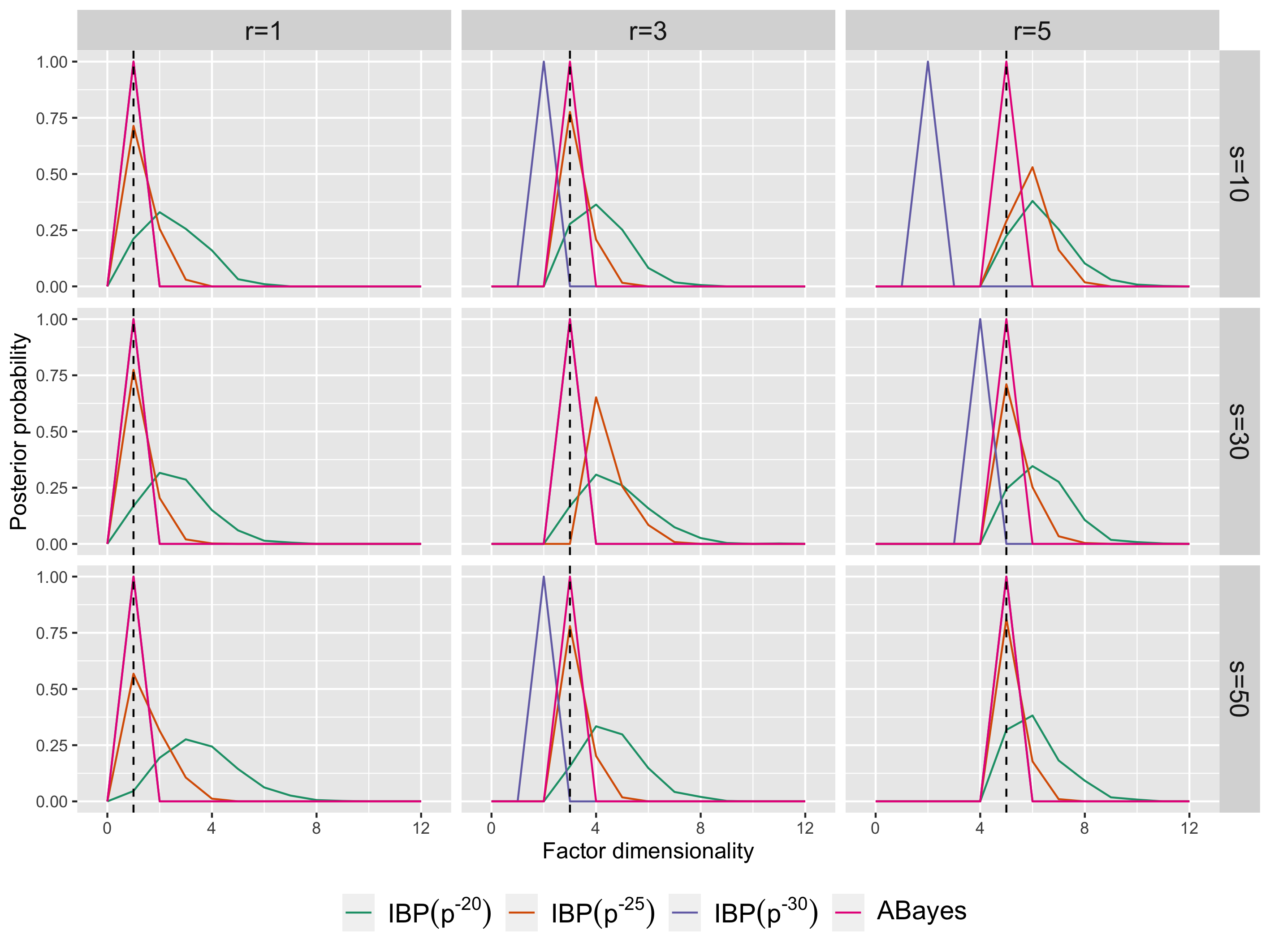
Figure 1: Posterior distributions of the factor dimensionality for the proposed adaptive Bayesian (AdaSS) prior and spike and slab with the two-parameter IBP prior with various $\alpha$ (IBP($\alpha$)). The black dashed vertical lines indicate the true factor dimensionality $r$.

4.1.2 Comparison with frequentist estimators

In this simulation, we compare the performance of the AdaSS prior with some frequentist estimators for point estimation of the factor dimensionality. For our Bayesian model, we use the mode of the posterior distribution of the factor dimensionality as a point estimator. We consider the following five frequentist estimators as competitors: with $\mathbf{S}$ and $\mathbf{R}$ being the sample covariance and correlation matrices, respectively, and $r_{\max}\in[p]$ pre-specified,

• Eigenvalue threshold estimator (ET, Onatski (2010))

  $$\hat{r}_{\textsc{ET}}\mathrel{\mathop{\mathchar 58\relax}}=\sum_{j=1}^{p}\mathbbm{1}\mathinner{\left(\lambda_{j}(\mathbf{S})>w\lambda_{r_{\max}+1}(\mathbf{S})+(1-w)\lambda_{2r_{\max}+1}(\mathbf{S})\right)},$$

  where $w\mathrel{\mathop{\mathchar 58\relax}}=2^{2/3}(2^{2/3}-1).$

• Eigenvalue ratio estimator (ER, Ahn and Horenstein (2013); Lam and Yao (2012)):

  $$\hat{r}_{\textsc{ER}}\mathrel{\mathop{\mathchar 58\relax}}=\operatorname*{\arg\!\max}_{j\in[r_{\max}]}\lambda_{j}(\mathbf{S})/\lambda_{j+1}(\mathbf{S}).$$

• Growth ratio estimator (GR, Ahn and Horenstein (2013)):

  $$\hat{r}_{\textsc{GR}}\mathrel{\mathop{\mathchar 58\relax}}=\operatorname*{\arg\!\max}_{j\in[r_{\max}]}\frac{\log(L_{j-1}/L_{j})}{\log(L_{j}/L_{j+1})},$$

  where $L_{j}\mathrel{\mathop{\mathchar 58\relax}}=\sum_{t=j+1}^{p}\lambda_{t}(\mathbf{S})$.

• Adjusted correlation threshold estimator (ACT, Fan et al. (2020)):

  $$\hat{r}_{\textsc{ACT}}\mathrel{\mathop{\mathchar 58\relax}}=\max\mathinner{\left\{j\in[r_{\max}]\mathrel{\mathop{\mathchar 58\relax}}\lambda_{j}^{\dagger}>1+\sqrt{p/(n-1)}\right\}},$$

  where

  $$\lambda_{j}^{\dagger}\mathrel{\mathop{\mathchar 58\relax}}=\mathinner{\left[\frac{1-w_{j}}{\hat{\lambda}_{j}}-\frac{w_{j}}{p-j}\mathinner{\left\{\sum_{t=j+1}^{p}(\hat{\lambda}_{t}-\hat{\lambda}_{j})^{-1}+4(\hat{\lambda}_{j+1}-\hat{\lambda}_{j})^{-1}\right\}}\right]}^{-1}$$

  with $\hat{\lambda}_{j}\mathrel{\mathop{\mathchar 58\relax}}=\lambda_{j}(\mathbf{R})$ and $w_{j}\mathrel{\mathop{\mathchar 58\relax}}=(p-j)/(n-1)$ for $j\in[p].$

• Diagonal thresholding estimator (DT, Cai et al. (2013)):

  $$\hat{r}_{\textsc{DT}}\mathrel{\mathop{\mathchar 58\relax}}=\max\mathinner{\left\{j\in[r_{\max}]\mathrel{\mathop{\mathchar 58\relax}}\lambda_{j}(\check{\mathbf{S}}_{[J,J]})>2\mathinner{\left(1+\sqrt{|J|/n}+\sqrt{(2(1+|J|)\log(\textup{e}p)+6\log n)/n}\right)}^{2}\right\}},$$

  where $\check{\mathbf{S}}\mathrel{\mathop{\mathchar 58\relax}}=n^{-1}\sum_{i=1}^{n}(\mathbf{Y}_{i}+\mathbf{Z}^{0}_{i})(\mathbf{Y}_{i}+\mathbf{Z}^{0}_{i})^{\top}$ with $\mathbf{Z}^{0}_{1},\dots,\mathbf{Z}^{0}_{n}\stackrel{{\scriptstyle\textup{iid}}}{{\sim}}\texttt{{N}}(\mathbf{0},\mathbf{I})$ and

  $$J\mathrel{\mathop{\mathchar 58\relax}}=\mathinner{\left\{j\in[p]\mathrel{\mathop{\mathchar 58\relax}}\check{\mathbf{S}}_{[j,j]}\geq 2+6\sqrt{\log p/n}\right\}}.$$

We fix $r_{\max}=10$ throughout the simulation study.

A synthetic data set of size $n$ is generated from the $p$-dimensional normal distribution with mean $\mathbf{0}$ and covariance $\mathbf{B}^{\star}(\mathbf{B}^{\star})^{\top}+\mathbf{I}$, where the true loading matrix $\mathbf{B}^{\star}\in\mathbb{R}^{p\times r}$ is $s$-sparse. The true loading matrix $\mathbf{B}^{\star}$ is generated as follows: we first select $s$ nonzero rows and sample the elements in the nonzero rows from the uniform distribution on $[-4/\sqrt{s},-3/\sqrt{s}]\cup[3/\sqrt{s},4/\sqrt{s}]$. We take two sample sizes $n=50$ and $n=100$. We fix the dimension $p=1,000$ and let the sparsity $s$ and factor dimensionality $r$ vary among $s\in\{10,30,50\}$ and $r\in\{1,3,5\}$, respectively.

The simulation results based on 100 synthetic data sets of size $n=50$ and $n=100$ are summarized in Tables 1 and 2, respectively. We see that the proposed Bayesian model with the AdaSS prior outperforms the other competitors in the estimation of the factor dimensionality. The AdaSS prior has the highest proportion of the correct estimation for 17 out of the total 18 simulation setups. In particular, there are considerable performance gaps between the AdaSS prior and the other competitors when sparsity is small ($s=10$) or the factor dimensionality is large ($r=5$).

Table 1: Proportions of correct estimation (“True”), overestimation (“Over”) and underestimation (“Under”) of the estimated factor dimensionalities for various sparsity $s$ and true factor dimensionality $r$ obtained on 100 synthetic data sets of size $n=50$. “Ave” is the average of the estimated factor dimensionalities.

$s$	$r$		ET	ER	GR	ACT	DT	AdaSS
10	1	True	85	97	97	96	100	100
		Over	14	3	3	4	0	0
		Under	1	0	0	0	0	0
		Ave	1.14	1.03	1.03	1.04	1	1
	3	True	24	3	3	0	0	97
		Over	1	0	0	0	0	0
		Under	75	97	97	100	100	3
		Ave	2.16	1.35	1.37	1.01	1	2.97
	5	True	0	0	0	0	0	77
		Over	0	0	0	0	0	15
		Under	100	100	100	100	100	8
		Ave	2.97	1.54	1.55	1.01	1.1	5.06
30	1	True	86	96	97	97	100	100
		Over	12	4	3	3	0	0
		Under	2	0	0	0	0	0
		Ave	1.1	1.1	1.07	1.03	1	1
	3	True	46	15	15	0	0	94
		Over	0	0	0	0	0	0
		Under	54	85	85	100	100	6
		Ave	2.43	1.57	1.57	1.09	1	2.93
	5	True	0	1	1	0	0	87
		Over	0	0	0	0	0	0
		Under	100	99	99	100	100	13
		Ave	3.2	1.72	1.77	1.06	1	4.86
50	1	True	80	98	97	95	100	100
		Over	17	2	3	5	0	0
		Under	3	0	0	0	0	0
		Ave	1.17	1.04	1.05	1.05	1	1
	3	True	58	9	10	6	0	73
		Over	2	0	0	0	0	0
		Under	40	91	90	94	100	27
		Ave	2.62	1.52	1.56	1.4	1	2.67
	5	True	2	2	2	0	0	61
		Over	0	0	0	0	0	0
		Under	98	98	98	100	100	39
		Ave	3.39	1.94	1.99	1.25	1	4.54

Table 2: Proportions of correct estimation (“True”), overestimation (“Over”) and underestimation (“Under”) of the estimated factor dimensionalities for various sparsity $s$ and true factor dimensionality $r$ obtained on 100 synthetic data sets of size $n=100$. “Ave” is the average of the estimated factor dimensionalities.

$s$	$r$		ET	ER	GR	ACT	DT	AdaSS
10	1	True	78	100	100	93	100	100
		Over	22	0	0	7	0	0
		Under	0	0	0	0	0	0
		Ave	1.24	1	1	1.07	1	1
	3	True	66	9	10	0	0	86
		Over	2	0	0	0	0	13
		Under	32	91	90	100	100	1
		Ave	2.7	1.55	1.57	1.02	1.25	3.12
	5	True	6	0	0	0	0	20
		Over	0	0	0	0	0	77
		Under	94	100	100	100	100	3
		Ave	3.63	1.83	1.86	1	2.13	5.93
30	1	True	83	100	100	93	100	100
		Over	17	0	0	7	0	0
		Under	0	0	0	0	0	0
		Ave	1.18	1	1	1.09	1	1
	3	True	92	33	34	5	0	99
		Over	4	0	0	2	0	1
		Under	4	67	66	93	100	0
		Ave	3	1.96	1.98	1.56	1	3.01
	5	True	46	3	4	0	0	68
		Over	1	0	0	0	0	32
		Under	53	97	96	100	100	0
		Ave	4.45	2	2.1	1.43	1	5.32
50	1	True	85	100	100	94	100	100
		Over	15	0	0	6	0	0
		Under	0	0	0	0	0	0
		Ave	1.16	1	1	1.06	1	1
	3	True	99	59	61	64	0	98
		Over	1	0	0	2	0	0
		Under	0	41	39	34	100	2
		Ave	3.01	2.36	2.38	2.67	1	2.98
	5	True	68	15	20	2	0	91
		Over	0	0	0	0	0	6
		Under	32	85	80	98	100	3
		Ave	4.68	2.36	2.65	2.61	1	5.03

4.1.3 Covariance matrix estimation

In this simulation study, we compare the AdaSS prior with other competitors for covariance matrix estimation. For competitors, we consider the principal orthogonal complement thresholding method (POET, Fan et al. (2013)), the variational inference method for Bayesian sparse PCA (SPCA-VI, Ning (2021)), the Bayesian sparse factor models with multiplicative gamma process shrinkage prior (MGPS, Bhattacharya and Dunson (2011)) and two maximum a posteriori estimators that employ the multi-scale generalized double Pareto prior (MDP, (Srivastava et al., 2017)) and the spike-and-slab lasso with Indian buffet process prior (SSL-IBP, (Rockova and George, 2016)), respectively. For the POET and SPCA-VI, the factor dimensionality must be selected in advance and we use the true factor dimensionality for this. We use the posterior mean of the covariance matrix as the point estimator for the MGPS and AdaSS priors.

We generate 100 synthetic data sets with sample size $n=50$ and $n=100$, respectively, and we report the averages of the scaled spectral norm losses $\mathinner{\lVert\hat{\bm{\Sigma}}-\bm{\Sigma}^{\star}\rVert}/\|\bm{\Sigma}^{\star}\|$ between the point estimate $\hat{\bm{\Sigma}}$ of each estimator and the true covariance matrix $\bm{\Sigma}^{\star}$ obtained over 100 synthetic data sets in Tables 3 and 4. The AdaSS prior performs generally well, while the POET, MGPS and MDP are significantly inferior. SSL-IBP is not much worse and performs best for the setups with $s=50.$

Table 3: The averages and standard errors of the scaled spectral norm losses of the estimators of the covariance matrix obtained on 100 synthetic data sets with $n=50$.

$s$	$r$	POET	SPCA-VI	MGPS	MDP	SSL-IBP	ABayes
10	1	2.366 (0.151)	0.245 (0.108)	2.591 (2.04)	2.103 (0.135)	0.689 (0.062)	0.233 (0.103)
	3	1.83 (0.254)	0.398 (0.12)	1.45 (0.863)	1.583 (0.212)	0.646 (0.094)	0.301 (0.113)
	5	1.59 (0.232)	0.422 (0.111)	1.195 (0.575)	1.271 (0.191)	0.696 (0.101)	0.335 (0.107)
30	1	2.375 (0.155)	0.772 (0.102)	1.945 (1.292)	2.104 (0.14)	0.699 (0.067)	0.624 (0.152)
	3	2.073 (0.202)	0.674 (0.117)	2.078 (1.309)	1.839 (0.184)	0.696 (0.063)	0.609 (0.172)
	5	1.868 (0.192)	0.644 (0.086)	1.551 (0.87)	1.649 (0.175)	0.684 (0.052)	0.631 (0.138)
50	1	2.345 (0.146)	0.901 (0.039)	2.018 (1.52)	2.072 (0.13)	0.759 (0.065)	0.847 (0.134)
	3	2.145 (0.194)	0.762 (0.102)	1.996 (1.168)	1.901 (0.175)	0.695 (0.069)	0.966 (0.208)
	5	2.013 (0.2)	0.744 (0.098)	1.519 (0.752)	1.786 (0.182)	0.709 (0.067)	1.049 (0.228)

Table 4: The averages and standard errors of the scaled spectral norm losses of the estimators of the covariance matrix obtained on 100 synthetic data sets with $n=100$.

$s$	$r$	POET	SPCA-VI	MGPS	MDP	SSL-IBP	ABayes
10	1	1.437 (0.108)	0.164 (0.064)	2.374 (1.123)	1.322 (0.101)	0.523 (0.048)	0.17 (0.066)
	3	1.136 (0.146)	0.274 (0.074)	1.565 (1.129)	1.044 (0.141)	0.483 (0.066)	0.218 (0.074)
	5	0.999 (0.151)	0.281 (0.069)	1.051 (0.407)	0.881 (0.135)	0.464 (0.057)	0.244 (0.075)
30	1	1.437 (0.09)	0.366 (0.105)	2.489 (1.124)	1.317 (0.085)	0.534 (0.053)	0.317 (0.088)
	3	1.28 (0.138)	0.449 (0.083)	2.187 (0.946)	1.175 (0.133)	0.533 (0.055)	0.353 (0.105)
	5	1.178 (0.116)	0.457 (0.079)	1.723 (1.618)	1.084 (0.109)	0.538 (0.059)	0.4 (0.087)
50	1	1.428 (0.095)	0.707 (0.112)	2.357 (1.226)	1.306 (0.09)	0.57 (0.065)	0.536 (0.133)
	3	1.328 (0.102)	0.628 (0.102)	2.236 (1.072)	1.219 (0.1)	0.547 (0.058)	0.587 (0.133)
	5	1.261 (0.119)	0.57 (0.072)	1.729 (0.97)	1.161 (0.112)	0.564 (0.059)	0.652 (0.123)

4.2 Real data analysis

In this section, we analyze gene expression data on aging in mice from the AGEMAP (Atlas of Gene Expression in Mouse Aging Project) database Zahn et al. (2007). We obtained this data from the online website http://statweb.stanford.edu/$\sim$owen/data/AGEMAP. There are 5 female and 5 male mice in each age group, where there are 4 age groups of 1, 6, 16 and 24 months. Thus there are $40$ mice in total. From each of 40 mice, 16 microarrays obtained from 16 different tissues were prepared, and from each microarray, gene expression levels of $8,932$ probes were measured. In this paper, we focus only on the microarray data from the cerebrum tissue, for which the rotation test of Perry and Owen (2010) provided strong evidence for the presence of the latent factor. We will call this one tissue data set with sample size $n=40$ and dimension $p=8,932$ the AGEMAP data for simplicity.

We preprocessed the AGEMAP data following the regression model of Perry and Owen (2010). We obtained the mean-centered data by regressing out an intercept, sex, and age effects on each of the 8,932 outcomes. Then the factor dimensionality is estimated based on the mean-centered data set. We consider the factor model with heterogeneous noise variances and impose the AdaSS prior presented in Remark 2.1. We set $q=10\geq\sqrt{n}=\sqrt{40}$, $A=0.1$ and $\mathbf{a}_{j}=(0.01,0.01)$ for every $j\in[p]$ in the prior. Then we take the posterior mode of the factor dimensionality as the point estimate. For comparison, we also considered the five frequentist methods described in Section 4.1, i.e., ET, ER, GR, ACT and DT.

Table 5 provides the factor dimensionality estimates by the proposed Bayesian model and the five competing frequentist methods. The four methods including the AdaSS prior estimate the factor dimensionality by 1. The presence of the one-dimensional latent factor was advocated by the rotation test of Perry and Owen (2010).

Figure 2(a) shows the histogram of the posterior means of the latent factors $\mathsf{E}(Z_{ik^{*}}|\mathbf{Y}_{1\mathrel{\mathop{\mathchar 58\relax}}n})$ for $i\in[n]$ obtained under the AdaSS prior, where $k^{*}$ denotes the index of the nonzero column of the loading matrix, i.e., $\mathbf{B}_{[\mathrel{\mathop{\mathchar 58\relax}},k^{*}]}\neq\mathbf{0}$ under the posterior distribution. The bimodality of the histogram is clearly shown, which is also confirmed by Perry and Owen (2010). Figure 2(b) presents the posterior distribution of the sparsity $|\textup{{supp}}(\mathbf{B})|$ of the loading matrix, which ranges from 79.4% to 82%. A similar 78% sparsity of the estimated factor model was reported by Rockova and George (2016).

Table 5: Estimated factor dimensionality for the AGEMAP data.

ET	ER	GR	ACT	DT	AdaSS
8	1	1	10	1	1

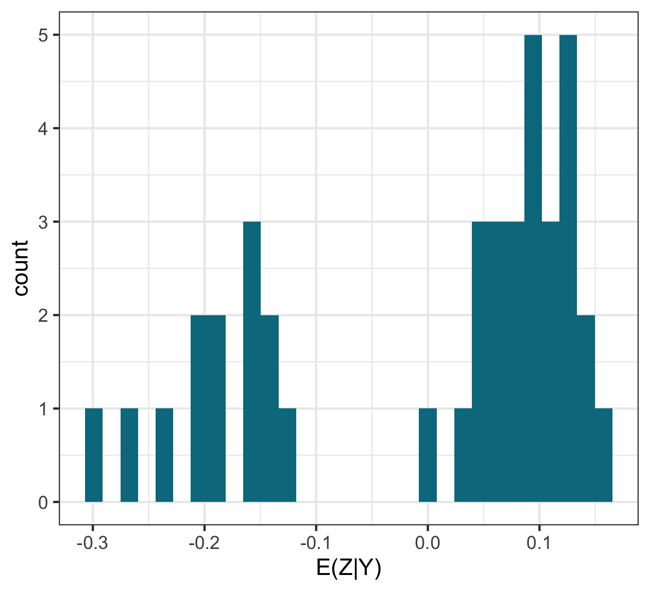
(a)

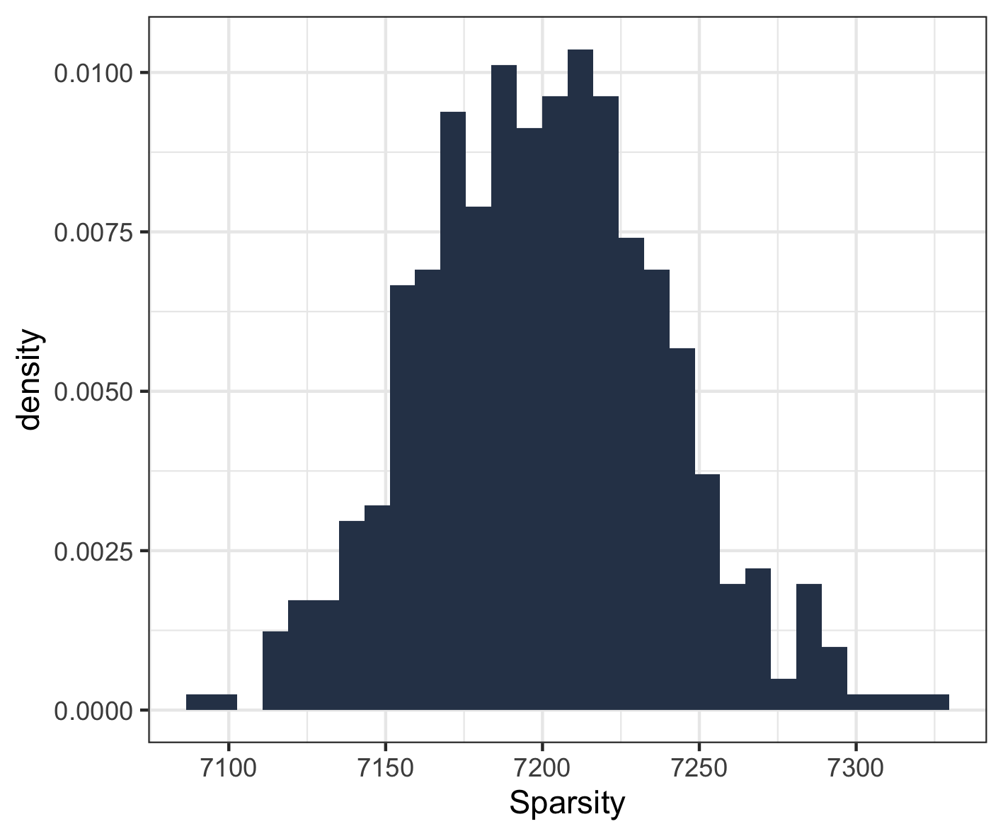
(b)

Figure 2: (a) Histogram of the posterior means of the latent factors for each observation; (b) Posterior distribution of the sparsity of the loading matrix for the AGEMAP data.

5 Concluding remarks

In this paper, we proposed a novel prior distribution, called AdaSS, to infer high-dimensional sparse factor models. We proved that the resulting posterior distribution asymptotically concentrates at the true factor dimensionality without knowing the sparsity level of the true loading matrix. This adaptivity to the sparsity is a remarkable advantage of the proposed method over other theoretically consistent estimators such as the point estimator in Cai et al. (2015) and Bayesian posterior distribution in Ohn and Kim (2022). We also showed that the proposed model attained the optimal detection rate of the eigengap for consistent estimation of the factor dimensionality. Moreover, the concentration rate of the posterior distribution of the covariance matrix is optimal when the true factor dimensionality is bounded and equal or faster than those of other Bayesian models otherwise. Our numerical studies amply confirmed the theoretical results and provided strong empirical support to the proposed AdaSS prior.

With our prior, nonzero row vectors of the loading matrix $\mathbf{B}$ are not sparse. That is, when $s^{\prime}$-many nonzero row vectors and the factor dimensionality are given, all the entries of the corresponding $s^{\prime}\times\xi$ sub-matrix are all nonzero. In practice, one may want to have sparsity in nonzero row vectors. Our prior can be modified easily to ensure such sparsity without hampering the asymptotic properties, which we will report somewhere else.

There are several promising directions for future work. In this paper, we consider the static factor model where the observations are assumed to be identically distributed. However, this static factor model may be inadequate to capture the dependence structure in some types of data, e.g., time series data. As an alternative, we may consider a dynamic factor model, where the covariance matrix as well as the factor dimensionality can be different at each time point. It would of interest to study the posterior consistency of the factor dimensionality which possibly varies over time. Another promising avenue of research is to develop the Bayesian factor model which deals with non-Gaussian or mixed-type observed variables. We believe that the proposed Bayesian model can be easily extended to those types of data using the Gaussian copula factor model developed by Murray et al. (2013). It would be interesting to investigate the theoretical properties of such a non-Gaussian extension of the proposed Bayesian model.

In this supplementary material, we provide proofs of the main results and additional numerical results.

Appendix A Proofs

Before giving the proofs, we introduce some additional notations. We define

$$\bar{\mathcal{C}}(p,q)\mathrel{\mathop{\mathchar 58\relax}}=\mathinner{\left\{\bm{\Sigma}=\mathbf{B}\mathbf{B}^{\top}+\psi\mathbf{I}\mathrel{\mathop{\mathchar 58\relax}}\mathbf{B}\in\mathbb{R}^{p\times q},\psi>0\right\}}$$

for $q\in\mathbbm{N}$. Note that the set $\bar{\mathcal{C}}(p,q)$ includes the support of the AdaSS prior.

A.1 Proofs of Theorems 3.4 and 3.8

Note that

$$\mathsf{P}_{\bm{\Sigma}^{\star}}^{(n)}\Pi(\mathcal{U}|\mathbf{Y}_{1\mathrel{\mathop{\mathchar 58\relax}}n})=\mathsf{P}_{\bm{\Sigma}^{\star}}^{(n)}\frac{N_{n}(\mathcal{U})}{D_{n}}$$

for any measurable subset $\mathcal{U}\subset\bar{\mathcal{C}}(p)$, where we denote

$$N_{n}(\mathcal{U}) \mathrel{\mathop{\mathchar 58\relax}}=\int_{\mathcal{U}}\frac{\mathsf{p}_{\bm{\Sigma}}^{(n)}}{\mathsf{p}_{\bm{\Sigma}^{\star}}^{(n)}}(\mathbf{Y}_{1\mathrel{\mathop{\mathchar 58\relax}}n})\Pi(\textup{d}\bm{\Sigma}),$$

$$D_{n} \mathrel{\mathop{\mathchar 58\relax}}=\int\frac{\mathsf{p}_{\bm{\Sigma}}^{(n)}}{\mathsf{p}_{\bm{\Sigma}^{\star}}^{(n)}}(\mathbf{Y}_{1\mathrel{\mathop{\mathchar 58\relax}}n})\Pi(\textup{d}\bm{\Sigma}).$$

We will prove Theorems 3.4 and 3.8 by deriving a lower bound of $D_{n}$ and an upper bound of $N_{n}(\mathcal{U})$ for $\mathcal{U}$ related to Theorems.

The following lemma provides a high-probability lower bound of $D_{n}$. The proof is deferred to Section B.1 in the supplementary material.

Lemma A.10.

Suppose that the prior distribution is defined through 2.1, 2.2 and 2.3 with $A>0$ and $\mathbf{a}\in\mathbb{R}_{+}^{2}$. Assume that $\lambda\lesssim s$. Then for any $\bm{\Sigma}^{\star}\in\mathcal{C}(p,r,s,\lambda,0)$, we have

$$\mathsf{P}_{\bm{\Sigma}^{\star}}^{(n)}\mathinner{\left(D_{n}\geq\textup{e}^{-C_{1}s(r\log n\vee\log p)-Asr\log(p\vee n)}\right)}\geq 1-\frac{1}{\log n}$$ (A.1)

for some universal constant $C_{1}>0$.

We now prove Theorems 3.4 and 3.8. Since the proof of Theorem 3.4 uses the result of Theorem 3.8, we first prove Theorem 3.8.

A.1.1 Proof of Theorem 3.8

Proof A.11 (Proof of Theorem 3.8).

Fix $\bm{\Sigma}^{\star}=\mathbf{B}^{\star}(\mathbf{B}^{\star})^{\top}+\psi^{\star}\mathbf{I}\in\mathcal{C}(p,r,s,\lambda,0)$. Recall that we let $\epsilon\mathrel{\mathop{\mathchar 58\relax}}=\lambda\sqrt{sr\log(p\vee n)/n}$. By Lemma A.10, there exists an universal constant $C_{1}>0$ such that $\mathsf{P}^{(n)}_{\bm{\Sigma}^{\star}}(\mathfrak{D}_{n})\geq 1-\log^{-1}n$ where

$$\mathfrak{D}_{n}\mathrel{\mathop{\mathchar 58\relax}}=\mathinner{\left\{\mathbf{Y}_{1\mathrel{\mathop{\mathchar 58\relax}}n}\in\mathbb{R}^{p\times n}\mathrel{\mathop{\mathchar 58\relax}}D_{n}\geq\textup{e}^{-C_{1}s(r\log n\vee\log p)-Asr\log(p\vee n)}\right\}}.$$ (A.2)

Note that

$$\Pi(|\textup{{supp}}(\mathbf{B})|>t)=\Pi(\|\mathbf{u}\|_{0}>t)\lesssim\sum_{t=\left\lceil{t}\right\rceil}^{p}\sum_{k=1}^{\infty}(p\vee n)^{-Atk}\lesssim\textup{e}^{-At\log(p\vee n)}$$

for any $t\in\mathbbm{N}.$ Hence, for a sufficiently large constant $C_{2}>0$, we have

$$\mathsf{P}_{\bm{\Sigma}^{\star}}^{(n)}\mathinner{\left[\Pi\mathinner{\left(|\textup{{supp}}(\mathbf{B})|>C_{2}sr|\mathbf{Y}_{1\mathrel{\mathop{\mathchar 58\relax}}n}\right)}\right]} \leq\mathsf{P}^{(n)}_{\bm{\Sigma}^{\star}}(\mathfrak{D}_{n}^{c})+\frac{\Pi\mathinner{\left(|\textup{{supp}}(\mathbf{B})|>C_{2}sr\right)}}{\textup{e}^{-C_{1}s(r\log n\vee\log p)-Asr\log(p\vee n)}}$$

$$\leq\log^{-1}n+\textup{e}^{C_{1}s(r\log n\vee\log p)-A(C_{2}-1)sr\log(p\vee n)}\to 0.$$

Therefore it suffices to show that $\mathsf{P}_{\bm{\Sigma}^{\star}}^{(n)}\mathinner{\left[\Pi(\mathcal{U}|\mathbf{Y}_{1\mathrel{\mathop{\mathchar 58\relax}}n})\right]}$ converges to zero, where

$$\mathcal{U}\mathrel{\mathop{\mathchar 58\relax}}=\mathinner{\left\{\bm{\Sigma}\in\bar{\mathcal{C}}(p,q)\mathrel{\mathop{\mathchar 58\relax}}|\textup{{supp}}(\mathbf{B})|\leq C_{2}sr,\mathinner{\lVert\bm{\Sigma}-\bm{\Sigma}^{\star}\rVert}\geq M\epsilon\right\}}.$$

We use the test function given in the next lemma to bound the posterior probability of $\mathcal{U}$. The proof of the lemma is provided in Section B.2 in the supplementary material.

Lemma A.12.

Let $\bm{\Sigma}^{\star}\mathrel{\mathop{\mathchar 58\relax}}=\mathbf{B}^{\star}(\mathbf{B}^{\star})^{\top}+\psi^{\star}\mathbf{I}\in\mathcal{C}(p,r,s,\lambda,0)$ and define a set

$$H_{1}\mathrel{\mathop{\mathchar 58\relax}}=\mathinner{\left\{\bm{\Sigma}\in\bar{\mathcal{C}}(p,q)\mathrel{\mathop{\mathchar 58\relax}}|\textup{{supp}}(\mathbf{B})|\leq t,\mathinner{\lVert\bm{\Sigma}-\bm{\Sigma}^{\star}\rVert}\geq M\tilde{\epsilon}\right\}},$$

where $t\in\mathbbm{N}$, $q\in\mathbbm{N}$, $M>2^{4/3}$ and $\tilde{\epsilon}>0$. Then there exists a test function $\phi\mathrel{\mathop{\mathchar 58\relax}}\mathbb{R}^{p\times n}\mapsto[0,1]$ such that

$$\mathsf{P}^{(n)}_{\bm{\Sigma}^{\star}}\phi(\mathbf{Y}_{1\mathrel{\mathop{\mathchar 58\relax}}n}) \leq 3\exp\mathinner{\left(2t\log p+(C_{3}+1)(t+s)-\frac{C_{3}M^{1/2}}{(1+\psi_{0}^{-2})\lambda^{2}}n\tilde{\epsilon}^{2}\right)},$$

$$\sup_{\bm{\Sigma}\mathrel{\mathop{\mathchar 58\relax}}\bm{\Sigma}\in H_{1}}\mathsf{P}^{(n)}_{\bm{\Sigma}}(1-\phi(\mathbf{Y}_{1\mathrel{\mathop{\mathchar 58\relax}}n})) \leq\exp\mathinner{\left(C_{3}(t+s)-\frac{C_{3}M}{4}n\tilde{\epsilon}^{2}\right)}$$

for some universal constant $C_{3}>0$.

For the test function $\phi$ given in Lemma A.12 and the set $\mathfrak{D}_{n}$ defined in A.2, we have

$$\mathsf{P}^{(n)}_{\bm{\Sigma}^{\star}}\mathinner{\left[\Pi\mathinner{\left(\mathcal{U}|\mathbf{Y}_{1\mathrel{\mathop{\mathchar 58\relax}}n}\right)}\right]} \leq\mathsf{P}^{(n)}_{\bm{\Sigma}^{\star}}\phi+\mathsf{P}^{(n)}_{\bm{\Sigma}^{\star}}\mathinner{\left[(1-\phi)\Pi\mathinner{\left(\mathcal{U}|\mathbf{Y}_{1\mathrel{\mathop{\mathchar 58\relax}}n}\right)}\mathbbm{1}(\mathfrak{D}_{n})\right]}+\mathsf{P}_{\bm{\Sigma}^{\star}}(\mathfrak{D}_{n}^{c})$$

$$\leq 3\textup{e}^{C_{4}sr\log p-C_{5}M^{1/2}n\epsilon^{2}/\lambda}+\textup{e}^{C_{6}sr\log(p\vee n)-C_{7}Mn\epsilon^{2}}+\log^{-1}n$$

$$\leq 3\textup{e}^{(C_{8}-C_{9}M^{1/2})sr\log(p\vee n)}+\log^{-1}n$$

for some universal positive constants $C_{4},\dots,C_{9}$. Hence, we obtain the desired result by choosing sufficiently large $M>0$.

A.1.2 Proof of Theorem 3.4

Proof A.13 (Proof of 3.3).

Fix $\bm{\Sigma}^{\star}=\mathbf{B}^{\star}(\mathbf{B}^{\star})^{\top}+\psi^{\star}\mathbf{I}\in\mathcal{C}(p,r,s,\lambda,\zeta)$. We first show that the expectation of the posterior probability of the event $\mathinner{\left\{\bm{\Sigma}\in\bar{\mathcal{C}}(p,q)\mathrel{\mathop{\mathchar 58\relax}}\xi(\mathbf{B})<r\right\}}$ converges to zero. converges to zero. For this, it suffices to show that

$$\mathinner{\left\{\bm{\Sigma}\in\bar{\mathcal{C}}(p,q)\mathrel{\mathop{\mathchar 58\relax}}\xi(\mathbf{B})<r\right\}}\subset\mathinner{\left\{\bm{\Sigma}\in\bar{\mathcal{C}}(p,q)\mathrel{\mathop{\mathchar 58\relax}}\mathinner{\!\left\lVert\bm{\Sigma}-\bm{\Sigma}^{\star}\right\rVert}>\zeta/2\right\}}$$ (A.3)

due to Theorem 3.8. Suppose that $\xi(\mathbf{B})<r$. Since $\mathbf{B}^{\star}$ is of full rank, there exists $\mathbf{w}_{1}\in\textup{{span}}(\mathbf{B})^{\perp}\cap\textup{{span}}(\mathbf{B}^{\star})$ with $\mathinner{\!\left\lVert\mathbf{w}_{1}\right\rVert}_{2}=1$. For such $\mathbf{w}_{1}$, we have

$$\mathinner{\!\left\lVert\mathbf{B}\mathbf{B}^{\top}-\mathbf{B}^{\star}(\mathbf{B}^{\star})^{\top}\right\rVert} \geq\mathinner{\!\left\lVert\mathinner{\left(\mathbf{B}\mathbf{B}^{\top}-\mathbf{B}^{\star}(\mathbf{B}^{\star})^{\top}\right)}\mathbf{w}_{1}\right\rVert}_{2}$$

$$=\mathinner{\!\left\lVert\mathbf{B}^{\star}(\mathbf{B}^{\star})^{\top}\mathbf{w}_{1}\right\rVert}_{2}\geq\zeta.$$

Let $\mathcal{J}\mathrel{\mathop{\mathchar 58\relax}}=\textup{{span}}(\mathbf{B})\cup\textup{{span}}(\mathbf{B}^{\star})$. Since $\textup{{rank}}(\mathcal{J})<2r\leq p$, there exists $\mathbf{w}_{2}\in\mathcal{J}^{\perp}$ with $\mathinner{\!\left\lVert\mathbf{w}_{2}\right\rVert}_{2}=1$. Then $\mathinner{\!\left\lVert\bm{\Sigma}-\bm{\Sigma}^{\star}\right\rVert}\geq\mathinner{\!\left\lVert\mathinner{\left(\bm{\Sigma}-\bm{\Sigma}^{\star}\right)}\mathbf{w}_{2}\right\rVert}_{2}=\mathinner{\!\left\lvert\psi-\psi^{\star}\right\rvert}$. By the triangular inequality, we obtain

$$\mathinner{\!\left\lVert\mathbf{B}\mathbf{B}^{\top}-\mathbf{B}^{\star}(\mathbf{B}^{\star})^{\top}\right\rVert}\leq\mathinner{\!\left\lVert\bm{\Sigma}-\bm{\Sigma}^{\star}\right\rVert}+\mathinner{\lVert\mathinner{(\psi-\psi^{\star})}\mathbf{I}\rVert}\leq 2\mathinner{\!\left\lVert\bm{\Sigma}-\bm{\Sigma}^{\star}\right\rVert},$$ (A.4)

which proves A.3. By the assumption that $\zeta\geq c_{0}\epsilon$ for sufficiently large $c_{0}>0$, it follows that $\mathsf{P}_{\bm{\Sigma}^{\star}}^{(n)}\Pi(\xi(\mathbf{B})<r|\mathbf{Y}_{1\mathrel{\mathop{\mathchar 58\relax}}n})\to 0$ from Theorem 3.8.

For the event $\mathinner{\left\{\bm{\Sigma}\in\bar{\mathcal{C}}(p,q)\mathrel{\mathop{\mathchar 58\relax}}\xi(\mathbf{B})>(1+\delta)r\right\}}$, we use the bound

$$\mathsf{P}_{\bm{\Sigma}^{\star}}^{(n)}\Pi\mathinner{\left(\xi(\mathbf{B})>(1+\delta)r|\mathbf{Y}_{1\mathrel{\mathop{\mathchar 58\relax}}n}\right)}\leq T_{1}+T_{2},$$ (A.5)

where we denote

$$T_{1} \mathrel{\mathop{\mathchar 58\relax}}=\mathsf{P}_{\bm{\Sigma}^{\star}}^{(n)}\Pi\mathinner{\left(\xi(\mathbf{B})>(1+\delta)r,|\textup{{supp}}(\mathbf{B})|\geq s|\mathbf{Y}_{1\mathrel{\mathop{\mathchar 58\relax}}n}\right)}$$

$$T_{2} \mathrel{\mathop{\mathchar 58\relax}}=\mathsf{P}_{\bm{\Sigma}^{\star}}^{(n)}\Pi\mathinner{\left(|\textup{{supp}}(\mathbf{B})|<s|\mathbf{Y}_{1\mathrel{\mathop{\mathchar 58\relax}}n}\right)}.$$

For $T_{1}$, note that

$$\Pi\mathinner{\left(\xi(\mathbf{B})>(1+\delta)r,|\textup{{supp}}(\mathbf{B})|\geq s\right)} \leq\Pi(\|\mathbf{u}\|_{0}\geq s,\|\mathbf{v}\|_{0}>(1+\delta)r)$$

$$\lesssim\sum_{k\in[q]\mathrel{\mathop{\mathchar 58\relax}}k>(1+\delta)r}\sum_{t\in[p]\mathrel{\mathop{\mathchar 58\relax}}t\geq s}\textup{e}^{-Atk\log(p\vee n)}$$

$$\lesssim\textup{e}^{-A(1+\delta)sr\log(p\vee n)}.$$

Hence, by Lemma A.10, there exist constants $C_{1}>0$ and $C_{2}>0$ such that

$$T_{1} \leq\mathsf{P}^{(n)}_{\bm{\Sigma}^{\star}}(\mathfrak{D}_{n}^{c})+\mathsf{P}_{\bm{\Sigma}^{\star}}^{(n)}\mathinner{\left[\Pi\mathinner{\left(\xi(\mathbf{B})>(1+\delta)r,|\textup{{supp}}(\mathbf{B})|\geq s|\mathbf{Y}_{1\mathrel{\mathop{\mathchar 58\relax}}n}\right)}\mathbbm{1}(\mathfrak{D}_{n})\right]}$$ (A.6)

$$\leq\log^{-1}n+\frac{\Pi\mathinner{\left(\xi(\mathbf{B})>(1+\delta)r,|\textup{{supp}}(\mathbf{B})|\geq s\right)}}{\exp\mathinner{\left(C_{1}s(r\log n\vee\log p)+Asr\log(p\vee n)\right)}}$$

$$\leq\log^{-1}n+\exp\mathinner{\left(C_{2}sr\log(p\vee n)-A\delta sr\log(p\vee n)\right)},$$

where $\mathfrak{D}_{n}\mathrel{\mathop{\mathchar 58\relax}}=\mathinner{\left\{\mathbf{Y}_{1\mathrel{\mathop{\mathchar 58\relax}}n}\in\mathbb{R}^{p\times n}\mathrel{\mathop{\mathchar 58\relax}}D_{n}\geq\textup{e}^{-C_{1}s(r\log n\vee\log p)-Asr\log(p\vee n)}\right\}}.$ Therefore, $T_{1}$ converges to zero if $A>C_{2}/\delta$. For $T_{2}$, we will show that

$$\mathinner{\left\{\bm{\Sigma}\in\bar{\mathcal{C}}(p,q)\mathrel{\mathop{\mathchar 58\relax}}|\textup{{supp}}(\mathbf{B})|<s\right\}}\subset\mathinner{\left\{\bm{\Sigma}\in\bar{\mathcal{C}}(p,q)\mathrel{\mathop{\mathchar 58\relax}}\mathinner{\!\left\lVert\bm{\Sigma}-\bm{\Sigma}^{\star}\right\rVert}>\zeta/2\right\}}.$$ (A.7)

Suppose that $|\textup{{supp}}(\mathbf{B})|<s$. Then $\mathcal{S}^{-}\mathrel{\mathop{\mathchar 58\relax}}=\textup{{supp}}(\mathbf{B}^{\star})\setminus\textup{{supp}}(\mathbf{B})$ is not empty, and so we can find $j^{*}\in[p]$ such that $j^{*}\in\mathcal{S}^{-}$. Let $\mathbf{w}_{3}\mathrel{\mathop{\mathchar 58\relax}}=(v_{3j})_{j\in[p]}$ be a vector such that $w_{3j^{*}}=1$ and $w_{3j}=0$ for $j\neq j^{*}$. Then since $\mathbf{B}_{[j^{*},\mathrel{\mathop{\mathchar 58\relax}}]}=\mathbf{0}$, we have

$$\mathinner{\!\left\lVert\mathbf{B}\mathbf{B}^{\top}-\mathbf{B}^{\star}(\mathbf{B}^{\star})^{\top}\right\rVert} \geq\mathinner{\!\left\lVert(\mathbf{B}\mathbf{B}^{\top}-\mathbf{B}^{\star}(\mathbf{B}^{\star})^{\top})\mathbf{w}_{3}\right\rVert}_{2}$$

$$=\mathinner{\!\bigl{\lVert}\mathbf{B}^{\star}\mathinner{\bigl{(}\mathbf{B}^{\star}_{[j^{*},\mathrel{\mathop{\mathchar 58\relax}}]}\bigr{)}}^{\top}\bigr{\rVert}}_{2}\geq\zeta$$

which, together with A.4, proves A.7. Thus Theorem 3.8 with the assumption $\zeta\geq c_{0}\epsilon$ implies that $T_{2}=o(1),$ which completes the proof.

Proof A.14 (Proof of 3.4).

It is sufficient to prove that

$$T_{1}^{*}\mathrel{\mathop{\mathchar 58\relax}}=\mathsf{P}_{\bm{\Sigma}^{\star}}^{(n)}\Pi\mathinner{\left(\xi(\mathbf{B})>r,|\textup{{supp}}(\mathbf{B})|\geq s|\mathbf{Y}_{1\mathrel{\mathop{\mathchar 58\relax}}n}\right)}\to 0.$$

Using a similar argument used in A.6, if $r\lesssim\log(p\vee n)/\log n$, we have that

$$T_{1}^{*} \leq\log^{-1}n+\exp\mathinner{\left(C_{1}s(r\log n\vee\log p)+Asr\log(p\vee n)-As(r+1)\log(p\vee n)\right)}$$

$$\leq\log^{-1}n+\exp\mathinner{\left(C_{3}s\log(p\vee n)-As\log(p\vee n)\right)},$$

for some $C_{3}>0$. Thus if $A>C_{3}$, we obtain the desired result.

A.2 Proof of Proposition 3.7

Proof A.15 (Proof of Proposition 3.7).

Let $\mathcal{W}(p,s)\mathrel{\mathop{\mathchar 58\relax}}=\mathinner{\left\{\mathbf{w}\in\{0,1\}^{p}\mathrel{\mathop{\mathchar 58\relax}}\|\mathbf{w}\|_{0}=s,w_{p}=0\right\}}$. For a given $\mathbf{w}\in\mathcal{W}(p,s)$, we define

$$\bm{\Sigma}(\mathbf{w})\mathrel{\mathop{\mathchar 58\relax}}=\frac{\lambda}{2}\mathbf{I}+\frac{\lambda}{2}\mathbf{e}_{p}\mathbf{e}_{p}^{\top}+\frac{\zeta}{s}\mathbf{w}\mathbf{w}^{\top},$$

where $\mathbf{e}_{p}$ is the vector of zeros except the $p$-th element which is equal to 1 and $\zeta>0$ is a constant such that $\zeta\leq\lambda/2$. Then, $\bm{\Sigma}(\mathbf{w})\in C(p,2,s,\lambda,\zeta)$. Thus, letting $\bm{\Sigma}_{0}\mathrel{\mathop{\mathchar 58\relax}}=\frac{\lambda}{2}(\mathbf{I}+\mathbf{e}_{p}\mathbf{e}_{p}^{\top})$ and

$$\mathcal{H}(p,s,\lambda,\zeta)\mathrel{\mathop{\mathchar 58\relax}}=\mathinner{\left\{\bm{\Sigma}(\mathbf{w})\mathrel{\mathop{\mathchar 58\relax}}\mathbf{w}\in\mathcal{W}(p,s)\right\}},$$

we have

$$\inf_{\hat{r}\mathrel{\mathop{\mathchar 58\relax}}\mathbb{R}^{p\times n}\mapsto\mathbbm{N}}\sup_{\bm{\Sigma}\in\mathcal{C}(p,r,s,\lambda,\zeta)}\mathsf{P}^{(n)}_{\bm{\Sigma}}\mathinner{\left(\hat{r}(\mathbf{Y}_{1\mathrel{\mathop{\mathchar 58\relax}}n})\neq r\right)}$$

$$\geq E_{p,s,\lambda,\zeta}\mathrel{\mathop{\mathchar 58\relax}}=\inf_{\phi\mathrel{\mathop{\mathchar 58\relax}}\mathbb{R}^{p\times n}\mapsto\{0,1\}}\mathinner{\left[\mathsf{P}^{(n)}_{\bm{\Sigma}_{0}}\mathinner{\left(\phi(\mathbf{Y}_{1\mathrel{\mathop{\mathchar 58\relax}}n})=1\right)}+\sup_{\bm{\Sigma}\in\mathcal{H}(p,s,\lambda,\zeta)}\mathsf{P}^{(n)}_{\bm{\Sigma}}\mathinner{\left(\phi(\mathbf{Y}_{1\mathrel{\mathop{\mathchar 58\relax}}n})=0\right)}\right]}.$$

To obtain a lower bound of $E_{p,s,\lambda,\zeta}$, we follow a standard argument of minimax theory. Let $\rho\mathrel{\mathop{\mathchar 58\relax}}=2\zeta/(s\lambda)$. Since $|\bm{\Sigma}(\mathbf{w})|=\lambda\mathinner{\left(\frac{\lambda}{2}+\zeta\right)}\mathinner{\left(\frac{\lambda}{2}\right)}^{p-2}$ and $|\bm{\Sigma}_{0}|=\lambda\mathinner{\left(\frac{\lambda}{2}\right)}^{p-1},$ the Kullback-Leibler (KL) divergence from $\mathsf{p}_{\bm{\Sigma}_{0}}^{(n)}$ to $\mathsf{p}_{\bm{\Sigma}(\mathbf{w})}^{(n)}$ is given by

$$\textup{{KL}}(\mathsf{p}_{\bm{\Sigma}(\mathbf{w})}^{(n)},\mathsf{p}_{\bm{\Sigma}_{0}}^{(n)}) =n\int\log(\frac{\mathsf{p}_{\bm{\Sigma}(\mathbf{w})}(\mathbf{y})}{\mathsf{p}_{\bm{\Sigma}_{0}}(\mathbf{y})})\mathsf{p}_{\bm{\Sigma}(\mathbf{w})}(\mathbf{y})\textup{d}\mathbf{y}$$

$$=\frac{n}{2}\textup{Tr}\mathinner{\left(\bm{\Sigma}(\mathbf{w})\bm{\Sigma}_{0}^{-1}-\mathbf{I}\right)}-\frac{n}{2}\log\mathinner{\!\bigl{\lvert}\bm{\Sigma}(\mathbf{w})\bm{\Sigma}_{0}^{-1}\bigr{\rvert}}$$

$$=\frac{n}{2}\mathinner{\left(\textup{Tr}\mathinner{\left(\rho\mathbf{w}\mathbf{w}^{\top}\right)}-\log\frac{\lambda/2+\zeta}{\lambda/2}\right)}$$

$$=\frac{n}{2}\mathinner{\left(\rho s-\log(1+\rho s)\right)}$$

$$\leq\alpha\mathrel{\mathop{\mathchar 58\relax}}=\frac{n}{4}\rho^{2}s^{2}=n\zeta^{2}/\lambda^{2}$$

for any $\mathbf{w}\in\mathcal{W}(p,s)$. Moreover, we have

$$M\mathrel{\mathop{\mathchar 58\relax}}=|\mathcal{H}(p,s,\lambda,\zeta)|=\binom{p-1}{s-1}\geq\mathinner{\left(\frac{p-1}{s-1}\right)}^{s-1}\geq\mathinner{\left(\frac{p}{s}\right)}^{s-1}\geq\mathinner{\left(\frac{p}{s}\right)}^{s/2}.$$

Thus, by Proposition 2.3 of Tsybakov [2008] with $\tau=1/M$,

$$E_{p,s,\lambda,\zeta} \geq\frac{1}{2}\mathinner{\left(1-\frac{\alpha+\sqrt{\alpha/2}}{\log M}\right)}$$

$$\geq\frac{1}{2}\mathinner{\left(1-(2+\sqrt{2})\frac{\alpha\vee 1}{s\log(p/s)}\right)}.$$

We take $\zeta\mathrel{\mathop{\mathchar 58\relax}}=a\lambda\sqrt{s\log(p/s)/n}$ with $a\leq a_{0}\mathrel{\mathop{\mathchar 58\relax}}=(4+2\sqrt{2})^{-1/2}$ so that $\alpha\leq a_{0}^{2}s\log(p/s)\leq s\log(p/s)/(4+2\sqrt{2})$ for sufficiently large $p$. Also, $\zeta\leq\lambda/2$ for all sufficiently large $n$ since $s\log p=o(n)$. Hence $E_{p,s,\lambda,\zeta}$ is further bounded below by $1/4$, which is the desired result.

Appendix B Proofs of lemmas in Appendix A

B.1 Proof of Lemma A.10

We first introduce two lemmas that will be used in the proofs.

Lemma B.16.

Let $\Pi$ be a distribution on $\mathbbm{S}_{++}^{p}$ and $\bm{\Sigma}^{\star}\in\mathbbm{S}_{++}^{p}$. For $n$ iid $p$-dimensional random variables $\mathbf{Y}_{1\mathrel{\mathop{\mathchar 58\relax}}n}\mathrel{\mathop{\mathchar 58\relax}}=(\mathbf{Y}_{1},\dots,\mathbf{Y}_{n})$, let us denote $D_{n}\mathrel{\mathop{\mathchar 58\relax}}=\int\frac{\mathsf{p}_{\bm{\Sigma}}^{(n)}}{\mathsf{p}_{\bm{\Sigma}^{\star}}^{(n)}}(\mathbf{Y}_{1\mathrel{\mathop{\mathchar 58\relax}}n})\Pi(\textup{d}\bm{\Sigma})$. Then for any $\eta\in(0,\lambda_{p}(\bm{\Sigma}^{\star})\wedge 1)$,

$$\mathsf{P}^{(n)}_{\bm{\Sigma}^{\star}}\mathinner{\left(D_{n}\geq\exp\mathinner{\left(-C_{1}\frac{n\eta^{2}\log\rho(\bm{\Sigma}^{\star})}{\lambda_{p}^{2}(\bm{\Sigma}^{\star})}\vee\frac{\eta\sqrt{n\log n}}{\lambda_{p}(\bm{\Sigma}^{\star})}\right)}\Pi\mathinner{\left(\left\|{\bm{\Sigma}-\bm{\Sigma}^{\star}}\right\|_{\textup{F}}<\eta\right)}\right)}\geq 1-\frac{1}{\log n}$$

for some universal constant $C_{1}>0$, where $\rho(\bm{\Sigma}^{\star})\mathrel{\mathop{\mathchar 58\relax}}=2\lambda_{1}(\bm{\Sigma}^{\star})/\lambda_{p}(\bm{\Sigma}^{\star})$

Proof B.17.

Fix $\eta\in(0,\lambda_{p}(\bm{\Sigma}^{\star})\wedge 1)$ and let $\mathcal{E}\mathrel{\mathop{\mathchar 58\relax}}=\mathinner{\left\{\left\|{\bm{\Sigma}-\bm{\Sigma}^{\star}}\right\|_{\textup{F}}<\eta\right\}}$. Let $\Pi(\cdot|\mathcal{E})\mathrel{\mathop{\mathchar 58\relax}}=\Pi(\cdot\cap\mathcal{E})/\Pi(\mathcal{E})$, which is the re-normalized restriction of $\Pi$ on $\mathcal{E}.$ By Jensen’s inequality,

$$\log\mathinner{\left(\frac{D_{n}}{\Pi(\mathcal{E})}\right)}\geq\int_{\mathcal{E}}\mathinner{\left\{\frac{n}{2}\log|\bm{\Sigma}^{\star}\bm{\Sigma}^{-1}|-\frac{1}{2}\sum_{i=1}^{n}\mathbf{Y}_{i}^{\top}(\bm{\Sigma}^{-1}-(\bm{\Sigma}^{\star})^{-1})\mathbf{Y}_{i}\right\}}\Pi(\textup{d}\bm{\Sigma}|\mathcal{E}).$$

Let $Q_{i}\mathrel{\mathop{\mathchar 58\relax}}=\mathbf{Y}_{i}^{\top}(\bm{\Sigma}^{-1}-(\bm{\Sigma}^{\star})^{-1})\mathbf{Y}_{i}$, $W_{i}\mathrel{\mathop{\mathchar 58\relax}}=Q_{i}-\mathsf{P}_{\bm{\Sigma}^{\star}}Q_{i}$ and $\bar{W}\mathrel{\mathop{\mathchar 58\relax}}=n^{-1}\sum_{i=1}^{n}W_{i}$. Note that $\mathsf{P}_{\bm{\Sigma}^{\star}}Q_{i}=\textup{Tr}(\bm{\Sigma}^{\star}\bm{\Sigma}^{-1}-\mathbf{I})$ and that, by Supplement Lemma 1.3 of Pati et al. [2014], for any $\eta\in(0,1)$ such that $\left\|{\bm{\Sigma}-\bm{\Sigma}^{\star}}\right\|_{\textup{F}}\leq\eta$ and $\eta<2\lambda_{p}(\bm{\Sigma}^{\star})$, we have

$$\log(|\bm{\Sigma}^{\star}\bm{\Sigma}^{-1}|)-\textup{Tr}(\bm{\Sigma}^{\star}\bm{\Sigma}^{-1}-\mathbf{I})\geq-C_{2}\frac{\eta^{2}\log\rho(\bm{\Sigma}^{\star})}{\lambda_{p}^{2}(\bm{\Sigma}^{\star})}$$

for some constant $C_{2}>0$. Therefore,

$$\log\mathinner{\left(\frac{D_{n}}{\Pi(\mathcal{E})}\right)} \geq\int_{\mathcal{E}}\mathinner{\left\{\frac{n}{2}\log|\bm{\Sigma}^{\star}\bm{\Sigma}^{-1}|-\textup{Tr}(\bm{\Sigma}^{\star}\bm{\Sigma}^{-1}-\mathbf{I})-\bar{W}\right\}}\Pi(\textup{d}\bm{\Sigma}|\mathcal{E})$$

$$\geq-C_{2}\frac{n\eta^{2}\log\rho(\bm{\Sigma}^{\star})}{2\lambda_{p}^{2}(\bm{\Sigma}^{\star})}-\frac{n}{2}\int\bar{W}\Pi(\textup{d}\bm{\Sigma}|\mathcal{E}).$$

It remains to derive the high-probability upper bound of $|\bar{W}|$. By the variance formula for quadratic forms of multivariate normal random vectors, we have

$$\mathsf{P}_{\bm{\Sigma}^{\star}}(W_{i}^{2})=2\textup{Tr}\mathinner{\left((\bm{\Sigma}^{-1}\bm{\Sigma}^{\star}-\mathbf{I})^{2}\right)}=2\mathinner{\lVert\bm{\Sigma}^{-1}\bm{\Sigma}^{\star}-\mathbf{I}\rVert}_{\textup{F}}^{2}.$$

Since $\left\|{\bm{\Sigma}-\bm{\Sigma}^{\star}}\right\|_{\textup{F}}^{2}=\left\|{\bm{\Sigma}(\bm{\Sigma}^{-1}\bm{\Sigma}^{\star}-\mathbf{I})}\right\|_{\textup{F}}^{2}\geq\lambda_{p}^{2}(\bm{\Sigma}^{\star})\left\|{\bm{\Sigma}^{-1}\bm{\Sigma}^{\star}-\mathbf{I}}\right\|_{\textup{F}}^{2}$, by Markov’s inequality, we have

$$\mathsf{P}^{(n)}_{\bm{\Sigma}^{\star}}\mathinner{\left(|\bar{W}|>\frac{\eta\sqrt{\log n}}{\sqrt{n}\lambda_{p}(\bm{\Sigma}^{\star})}\right)}\leq\frac{1}{\log n}$$

for all $\bm{\Sigma}\in\mathcal{E},$ which completes the proof.

Lemma B.18.

Assume that $\bm{\beta}\mathrel{\mathop{\mathchar 58\relax}}=(\beta_{1},\dots,\beta_{s})^{\top}$ is distributed as $\beta_{j}\stackrel{{\scriptstyle\textup{iid}}}{{\sim}}\texttt{{Lap}}(1)$ for $j\in[s]$. Then for any $\bm{\beta}_{0}\in\mathbb{R}^{s}$ and any $\epsilon>0$,

$$\mathsf{P}_{\texttt{{Lap}}(1)}^{(s)}(\mathinner{\!\left\lVert\bm{\beta}-\bm{\beta}_{0}\right\rVert}_{2}\leq\epsilon)\geq\textup{e}^{-\mathinner{\!\left\lVert\bm{\beta}_{0}\right\rVert}_{1}-\epsilon-s\log(s/\epsilon)}.$$

Proof B.19.

By a change of variables $\bm{\beta}-\bm{\beta}_{0}\to\bm{\beta}^{*}$, we have

$$\mathsf{P}_{\texttt{{Lap}}(1)}^{(s)}\mathinner{\left(\mathinner{\!\left\lVert\bm{\beta}-\bm{\beta}_{0}\right\rVert}_{1}\leq\epsilon\right)} =\int_{\mathinner{\!\left\lVert\bm{\beta}-\bm{\beta}_{0}\right\rVert}_{1}\leq\epsilon}\frac{1}{2}\textup{e}^{-\|\bm{\beta}\|_{1}}\textup{d}\bm{\beta}$$

$$\geq\textup{e}^{-\mathinner{\!\left\lVert\bm{\beta}_{0}\right\rVert}_{1}}\int_{\mathinner{\!\left\lVert\bm{\beta}^{*}\right\rVert}_{1}\leq\epsilon}\frac{1}{2}\textup{e}^{-\|\bm{\beta}^{*}\|_{1}}\textup{d}\bm{\beta}^{*}$$

$$=\textup{e}^{-\mathinner{\!\left\lVert\bm{\beta}_{0}\right\rVert}_{1}}\mathsf{P}_{\texttt{{Exp}}(1)}^{(s)}\mathinner{\left(\sum_{i=1}^{s}E_{i}\leq\epsilon\right)},$$

where $E_{1},\dots,E_{s}$ are iid random variables following exponential distribution with scale $1$. Since the random variable $\sum_{i=1}^{s}E_{i}$ follows the gamma distribution with shape $n$ and scale $1$, we have that

$$\mathsf{P}_{\texttt{{Exp}}(1)}^{(s)}\mathinner{\left(\sum_{i=1}^{s}E_{i}\leq\epsilon\right)} =\frac{1}{\Gamma(s)}\int_{0}^{\epsilon}x^{s-1}\textup{e}^{-x}\textup{d}x$$

$$\geq\frac{1}{(s-1)!}\textup{e}^{-\epsilon}\int_{0}^{\epsilon}x^{s-1}\textup{d}x=\frac{\epsilon^{s}}{s!}\textup{e}^{-\epsilon}.$$

The inequality $s!\leq s^{s}$ completes the proof.

Now we are ready to prove Lemma A.10.

Proof B.20 (Proof of Lemma A.10).

Since $\lambda(\bm{\Sigma}^{\star})\geq\psi_{0}$ and $\rho(\bm{\Sigma}^{\star})\lesssim\lambda\lesssim n,$ Lemma B.16 with $\eta\mathrel{\mathop{\mathchar 58\relax}}=\sqrt{sr/n}$ implies that

$$D_{n}\geq\exp\mathinner{\left(-C_{1}sr\log n\right)}\Pi\mathinner{\left(\left\|{\bm{\Sigma}-\bm{\Sigma}^{\star}}\right\|_{\textup{F}}\leq\eta\right)}$$

for some $C_{1}>0$ with $\mathsf{P}_{\bm{\Sigma}^{\star}}^{(n)}$-probability at least $1-\log^{-1}n$. Since $\mathbf{B}$ and $\psi$ are independent under the prior distribution,

$$\Pi\mathinner{\left(\left\|{\bm{\Sigma}-\bm{\Sigma}^{\star}}\right\|_{\textup{F}}\leq\eta\right)}\geq\Pi\left(\left\|{\mathbf{B}\mathbf{B}^{\top}-\mathbf{B}^{\star}(\mathbf{B}^{\star})^{\top}}\right\|_{\textup{F}}\leq\frac{\eta}{2}\right)\Pi\left(\sqrt{p}|\psi-\psi^{\star}|\leq\frac{\eta}{2}\right).$$

Since $\lambda\geq\psi^{\star}\geq\psi_{0}>0$, it follows that

$$\Pi\mathinner{\left(|\psi-\psi^{\star}|\leq\frac{\eta}{2\sqrt{p}}\right)} \geq\frac{\eta}{2\sqrt{p}}\min_{\psi\in[\psi^{\star}/2,3\psi^{\star}/2]}\frac{a_{2}^{a_{1}}}{\Gamma(a_{1})}\psi^{-a_{1}-1}\textup{e}^{-a_{2}/\psi}$$

$$\gtrsim(np)^{-1/2}\lambda^{-a_{1}-1}\textup{e}^{-2a_{2}/\psi_{0}}$$

$$\gtrsim\textup{e}^{-C_{2}\log(p\vee n)}$$

for some $C_{2}>0$. Let $\mathcal{S}^{\star}\mathrel{\mathop{\mathchar 58\relax}}=\textup{{supp}}(\mathbf{B}^{\star})$ and let $\mathcal{K}(\mathbf{v})\mathrel{\mathop{\mathchar 58\relax}}=\mathinner{\left\{k\in[q]\mathrel{\mathop{\mathchar 58\relax}}v_{k}=1\right\}}$ for $\mathbf{v}\in\Delta_{q}$. If $\textup{{supp}}(\mathbf{B})=\mathcal{S}^{\star}$ and $\|\mathbf{v}\|_{0}=r$, we have

$$\left\|{\mathbf{B}\mathbf{B}^{\top}-\mathbf{B}^{\star}(\mathbf{B}^{\star})^{\top}}\right\|_{\textup{F}} =\left\|{\mathbf{B}_{[\mathrel{\mathop{\mathchar 58\relax}},\mathcal{K}(\mathbf{v})}\mathbf{B}_{[\mathrel{\mathop{\mathchar 58\relax}},\mathcal{K}(\mathbf{v})]}^{\top}-\mathbf{B}^{\star}(\mathbf{B}^{\star})^{\top}}\right\|_{\textup{F}}$$

$$=\left\|{(\mathbf{B}_{[\mathrel{\mathop{\mathchar 58\relax}},\mathcal{K}(\mathbf{v})]}-\mathbf{B}^{\star})(\mathbf{B}_{[\mathrel{\mathop{\mathchar 58\relax}},\mathcal{K}(\mathbf{v})]}-\mathbf{B}^{\star})^{\top}+2\mathbf{B}^{\star}(\mathbf{B}_{[\mathrel{\mathop{\mathchar 58\relax}},\mathcal{K}(\mathbf{v})]}-\mathbf{B}^{\star})^{\top}}\right\|_{\textup{F}}$$

$$\leq\left\|{\mathbf{B}_{[\mathrel{\mathop{\mathchar 58\relax}},\mathcal{K}(\mathbf{v})]}-\mathbf{B}^{\star}}\right\|_{\textup{F}}^{2}+2\left\|{\mathbf{B}^{\star}(\mathbf{B}_{[\mathrel{\mathop{\mathchar 58\relax}},\mathcal{K}(\mathbf{v})]}-\mathbf{B}^{\star})^{\top}}\right\|_{\textup{F}}$$

$$\leq\left\|{\mathbf{B}_{[\mathcal{S}^{\star},\mathcal{K}(\mathbf{v})]}-\mathbf{B}^{\star}_{[\mathcal{S}^{\star},\mathrel{\mathop{\mathchar 58\relax}}]}}\right\|_{\textup{F}}^{2}+2\mathinner{\!\left\lVert\mathbf{B}^{\star}\right\rVert}\left\|{\mathbf{B}_{[\mathcal{S}^{\star},\mathcal{K}(\mathbf{v})]}-\mathbf{B}^{\star}_{[\mathcal{S}^{\star},\mathrel{\mathop{\mathchar 58\relax}}]}}\right\|_{\textup{F}}.$$

Therefore, since $\mathinner{\lVert\mathbf{B}^{\star}\rVert}=\lambda_{1}^{1/2}\mathinner{\bigl{(}\mathbf{B}^{\star}(\mathbf{B}^{\star})^{\top}\bigr{)}}\leq\lambda^{1/2}\lesssim\sqrt{s}$ by assumption, we have

$$\Pi \mathinner{\left(\left\|{\mathbf{B}\mathbf{B}^{\top}-\mathbf{B}^{\star}(\mathbf{B}^{\star})^{\top}}\right\|_{\textup{F}}\geq\eta/2\right)}$$

$$\geq\sum_{\mathbf{v}\mathrel{\mathop{\mathchar 58\relax}}\|\mathbf{v}\|_{0}=r}\Pi(\mathbf{u}^{\star},\mathbf{v})\Pi\mathinner{\left(\left\|{\mathbf{B}_{[\mathcal{S}^{\star},\mathcal{K}(\mathbf{v})]}-\mathbf{B}^{\star}_{[\mathcal{S}^{\star},\mathrel{\mathop{\mathchar 58\relax}}]}}\right\|_{\textup{F}}^{2}\geq C_{3}\sqrt{\frac{r}{n}}\big{|}\mathbf{u}=\mathbf{u}^{\star},\mathbf{v}\right)}$$

for some constant $C_{3}>0$, where $\mathbf{u}^{\star}\mathrel{\mathop{\mathchar 58\relax}}=(u_{j}^{\star})_{j\in[p]}$ is the binary vector such that $u_{j}^{\star}=1$ if $j\in\mathcal{S}^{\star}$ and $u_{j}^{\star}=0$ otherwise. By Lemma B.18, for $\|\mathbf{v}\|_{0}=r$, we have

$$\Pi \mathinner{\left(\left\|{\mathbf{B}_{[\mathcal{S}^{\star},\mathcal{K}(\mathbf{v})]}-\mathbf{B}^{\star}_{[\mathcal{S}^{\star},\mathrel{\mathop{\mathchar 58\relax}}]}}\right\|_{\textup{F}}^{2}\geq C_{3}\sqrt{\frac{r}{n}}\big{|}\mathbf{u}=\mathbf{u}^{\star},\mathbf{v}\right)}$$

$$\geq\exp\mathinner{\left(-C_{4}sr\log n-\mathinner{\!\bigl{\lVert}\mathbf{B}^{\star}_{[\mathcal{S}^{\star},\mathrel{\mathop{\mathchar 58\relax}}]}\bigr{\rVert}}_{1}\right)}\geq\textup{e}^{-C_{5}sr\log n}.$$

for some constants $C_{4}>0$ and $C_{5}>0$, where the second inequality follows from that

$$\mathinner{\!\bigl{\lVert}\mathbf{B}^{\star}_{[\mathcal{S}^{\star},\mathrel{\mathop{\mathchar 58\relax}}]}\bigr{\rVert}}_{1}= \mathinner{\!\bigl{\lVert}\mathbf{B}^{\star}\bigr{\rVert}}_{1}\leq\sqrt{sr}\mathinner{\!\bigl{\lVert}\mathbf{B}^{\star}\bigr{\rVert}}_{\textup{F}}$$

$$\leq\sqrt{s}r\mathinner{\!\bigl{\lVert}\mathbf{B}^{\star}\bigr{\rVert}}=\sqrt{s}r\lambda_{1}^{1/2}\mathinner{\left(\mathbf{B}^{\star}(\mathbf{B}^{\star})^{\top}\right)}\leq\sqrt{s\lambda}r\lesssim sr.$$

Lastly, we note that

$$\sum_{\mathbf{v}\mathrel{\mathop{\mathchar 58\relax}}\|\mathbf{v}\|_{0}=r}\Pi(\mathbf{u}^{\star},\mathbf{v})\gtrsim\textup{e}^{-Asr\log(p\vee n)}\frac{1}{\binom{p}{s}}\geq\textup{e}^{-Asr\log(p\vee n)-s\log p},$$

which completes the proof.

B.2 Proof of Lemma A.12

Proof B.21 (Proof of Lemma A.12).

We decompose $H_{1}$ as

$$H_{1}\subset\bigcup_{\mathcal{S}\mathrel{\mathop{\mathchar 58\relax}}|\mathcal{S}|\leq t}\mathinner{\left\{\bm{\Sigma}\in\bar{\mathcal{C}}(p,q)\mathrel{\mathop{\mathchar 58\relax}}\mathinner{\!\left\lVert\bm{\Sigma}-\bm{\Sigma}^{\star}\right\rVert}\geq M\epsilon,\textup{{supp}}(\mathbf{B})=\mathcal{S}\right\}}.$$

For a given loading matrix $\mathbf{B}$ with the support $\mathcal{S},$ let $\bar{\mathcal{S}}\mathrel{\mathop{\mathchar 58\relax}}=\mathcal{S}\cup\mathcal{S}^{\star}$, where $\mathcal{S}^{\star}\mathrel{\mathop{\mathchar 58\relax}}=\textup{{supp}}(\mathbf{B}^{\star})$. Define

$$\bm{\Sigma}_{\bar{\mathcal{S}}} \mathrel{\mathop{\mathchar 58\relax}}=\mathbf{B}_{[\bar{\mathcal{S}},\mathrel{\mathop{\mathchar 58\relax}}]}\mathbf{B}_{[\bar{\mathcal{S}},\mathrel{\mathop{\mathchar 58\relax}}]}^{\top}+\psi\mathbf{I},$$

$$\bm{\Sigma}^{\star}_{\bar{\mathcal{S}}} \mathrel{\mathop{\mathchar 58\relax}}=\mathbf{B}^{\star}_{[\bar{\mathcal{S}},\mathrel{\mathop{\mathchar 58\relax}}]}\mathinner{\left(\mathbf{B}^{\star}_{[\bar{\mathcal{S}},\mathrel{\mathop{\mathchar 58\relax}}]}\right)}^{\top}+\psi^{\star}\mathbf{I}.$$

Note that $\mathinner{\lVert\bm{\Sigma}_{\bar{\mathcal{S}}}-\bm{\Sigma}^{\star}_{\bar{\mathcal{S}}}\rVert}=\mathinner{\!\left\lVert\bm{\Sigma}-\bm{\Sigma}^{\star}\right\rVert}$ and so $H_{1}\subset\cup_{\mathcal{S}\mathrel{\mathop{\mathchar 58\relax}}|\mathcal{S}|\leq t}H_{1,\mathcal{S}},$ where we define

$$H_{1,\mathcal{S}}\mathrel{\mathop{\mathchar 58\relax}}=\mathinner{\left\{\bm{\Sigma}_{\bar{\mathcal{S}}}\in\mathbbm{S}_{+}^{|\bar{\mathcal{S}}|}\mathrel{\mathop{\mathchar 58\relax}}\mathinner{\lVert\bm{\Sigma}_{\bar{\mathcal{S}}}-\bm{\Sigma}^{\star}_{\bar{\mathcal{S}}}\rVert}\geq M\tilde{\epsilon}\right\}}.$$

We construct a test for $H_{0}\mathrel{\mathop{\mathchar 58\relax}}=\mathinner{\bigl{\{}\bm{\Sigma}_{\bar{\mathcal{S}}}^{\star}\bigr{\}}}$ versus $H_{1,\mathcal{S}}$. To do this, we use the following lemma from Gao and Zhou [2015].

Lemma B.22 (Lemma 5.7 of Gao and Zhou [2015]).

Let $\bm{\Sigma}_{0}\in\mathbbm{S}_{+}^{d}$. Then for any $M>0$ and $\tilde{\epsilon}>0$, there is a test function $\tilde{\phi}\mathrel{\mathop{\mathchar 58\relax}}\mathbb{R}^{d\times n}\mapsto[0,1]$ such that

$$\mathsf{P}_{\bm{\Sigma}_{0}}\tilde{\phi}(\mathbf{Y}_{1\mathrel{\mathop{\mathchar 58\relax}}n})\leq\exp\mathinner{\left(C_{1}d-\frac{C_{1}M^{2}}{4\mathinner{\!\left\lVert\bm{\Sigma}_{0}\right\rVert}^{2}}n\tilde{\epsilon}^{2}\right)}+2\exp(C_{1}d-C_{1}M^{1/2}n\tilde{\epsilon}^{2})$$

and

$$\sup_{\bm{\Sigma}_{1}\mathrel{\mathop{\mathchar 58\relax}}\mathinner{\!\left\lVert\bm{\Sigma}_{1}-\bm{\Sigma}_{0}\right\rVert}>M\tilde{\epsilon}}\mathsf{P}_{\bm{\Sigma}_{1}}^{(n)}(1-\tilde{\phi}(\mathbf{Y}_{1\mathrel{\mathop{\mathchar 58\relax}}n}))\leq\exp\mathinner{\left(C_{1}d-\frac{C_{1}M}{4}\mathinner{\left(1\vee\frac{M}{(M^{1/2}+2)^{2}\mathinner{\!\left\lVert\bm{\Sigma}_{0}\right\rVert}^{2}}\right)}n\tilde{\epsilon}^{2}\right)}$$

for some universal constant $C_{1}>0$.

By the above lemma together with the fact that $\mathinner{\lVert\bm{\Sigma}^{\star}_{\bar{\mathcal{S}}}\rVert}=\mathinner{\!\left\lVert\bm{\Sigma}^{\star}\right\rVert}\leq\lambda$, there exists a test function $\phi^{\mathcal{S}}$ which is a function of $\mathbf{Y}_{1[\bar{\mathcal{S}}]},\dots,\mathbf{Y}_{n[\bar{\mathcal{S}}]}$, such that for any $M>4^{2/3}$

$$\mathsf{P}^{(n)}_{\bm{\Sigma}^{\star}_{\bar{\mathcal{S}}}}\phi^{\mathcal{S}} \leq\exp\mathinner{\left(C_{1}|\bar{S}|-\frac{C_{1}M^{2}}{4\lambda^{2}}n\tilde{\epsilon}^{2}\right)}+2\exp(C_{1}|\bar{\mathcal{S}}|-C_{1}M^{1/2}n)$$

$$\leq 3\exp\mathinner{\left(C_{1}|\bar{\mathcal{S}}|-\frac{C_{1}M^{1/2}}{\lambda^{2}\vee 1}n\epsilon^{2}\right)}$$

and

$$\sup_{\bm{\Sigma}_{\bar{\mathcal{S}}}\mathrel{\mathop{\mathchar 58\relax}}\bm{\Sigma}_{\bar{\mathcal{S}}}\in H_{1,\mathcal{S}}}\mathsf{P}^{(n)}_{\bm{\Sigma}^{\bar{\mathcal{S}}}}(1-\phi^{\mathcal{S}}) \leq\exp\mathinner{\left(C_{1}|\bar{\mathcal{S}}|-\frac{C_{1}M}{4}n\tilde{\epsilon}^{2}\right)}.$$

We combine the tests by $\phi\mathrel{\mathop{\mathchar 58\relax}}=\max_{\mathcal{S}\mathrel{\mathop{\mathchar 58\relax}}|\mathcal{S}|\leq t}\phi^{\mathcal{S}}$. Since the test function $\phi^{\mathcal{S}}$ depends on the data $\mathbf{Y}_{1},\dots,\mathbf{Y}_{n}$ only through ($j\mathrel{\mathop{\mathchar 58\relax}}j\in\bar{\mathcal{S}}$)-th coordinates, we have $\mathsf{P}^{(n)}_{\bm{\Sigma}^{\star}}\phi^{\mathcal{S}}=\mathsf{P}^{(n)}_{\bm{\Sigma}^{\star}_{\bar{\mathcal{S}}}}\phi^{\mathcal{S}}$. Therefore, since $|\bar{\mathcal{S}}|\leq t+s$ for any $\mathcal{S}$ with $|\mathcal{S}|\leq t$, and $\lambda^{2}\vee 1\leq(1+1/\psi_{0}^{2})\lambda^{2},$ we have

$$\mathsf{P}^{(n)}_{\bm{\Sigma}^{\star}}\phi \leq\sum_{t=1}^{\left\lfloor{t}\right\rfloor}\binom{p}{t}3\exp\mathinner{\left(C_{1}(t+s)-\frac{C_{1}M^{1/2}}{\lambda^{2}\vee 1}n\tilde{\epsilon}^{2}\right)}$$

$$\leq 3(t+1)\textup{e}^{(t+1)\log p}\exp\mathinner{\left(C_{1}(t+s)-\frac{C_{1}M^{1/2}}{(1+\psi_{0}^{-2})\lambda^{2}}n\tilde{\epsilon}^{2}\right)}$$

$$\leq 3\exp\mathinner{\left(2t\log p+(C_{1}+1)(t+s)-\frac{C_{1}M^{1/2}}{(1+\psi_{0}^{-2})\lambda^{2}}n\tilde{\epsilon}^{2}\right)}$$

and

$$\sup_{\bm{\Sigma}\mathrel{\mathop{\mathchar 58\relax}}\bm{\Sigma}\in H_{1}}\mathsf{P}^{(n)}_{\bm{\Sigma}}(1-\phi) \leq\sup_{\mathcal{S}\mathrel{\mathop{\mathchar 58\relax}}|\mathcal{S}|\leq t}\sup_{\bm{\Sigma}_{\bar{\mathcal{S}}}\mathrel{\mathop{\mathchar 58\relax}}\bm{\Sigma}_{\bar{\mathcal{S}}}\in H_{1,\mathcal{S}}}\mathsf{P}^{(n)}_{\bm{\Sigma}_{\bar{\mathcal{S}}}}(1-\phi^{\mathcal{S}})$$

$$\leq\exp\mathinner{\left(C_{1}(t+s)-\frac{C_{1}M}{4}n\tilde{\epsilon}^{2}\right)},$$

which completes the proof.

Appendix C Additional numerical results

C.1 Convergence diagnostics

We assess the convergence of our MCMC samples via trace, autocorrelation and partial autocorrelation plots for some randomly selected nonzero loadings. Figure 3 presents such plots from the Bayesian factor model under the AdaSS prior for the AGEMAP data considered in Section 4.2. The results show that the MCMC chain converges well.

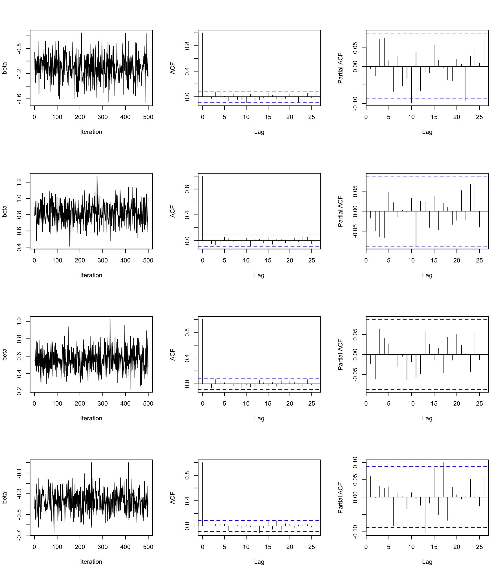
Figure 3: The trace, autocorrelation and partial autocorrelation plots of the posterior samples of some randomly selected nonzero loading for the AGEMAP data.

C.2 Application of the post-processing algorithm of Papastamoulis and Ntzoufras [2022]

In this section, we consider the estimation of the loading matrix from the MCMC samples of the proposed Bayesian model using the post-processing scheme of Papastamoulis and Ntzoufras [2022]. To illustrate this approach, we consider the following toy example, where we generate a dataset of size $n=100$ from the factor model with the sparse loading matrix $\mathbf{B}^{\star}=(\beta_{jk}^{\star})_{j\in[50],k\in[5]}\in\mathbb{R}^{50\times 5}$ having a “diagonal pattern” for non-sparse rows such that $\beta_{jk}^{\star}=1$ if $5(k-1)<j\leq 5k$ for $k\in[5]$ and $\beta_{jk}^{\star}=0$ otherwise (see Figure 4(a)). Figures 4(b) and 4(c) present the posterior means of the loading matrix computed before and after post-processing the MCMC samples, respectively. We can see that, without post-processing, the true pattern of the loading matrix is poorly recovered. For instance, the first and 6th columns are overlapped. But after post-processing, we are able to capture the true pattern up to a permutation of columns and signs of loadings.

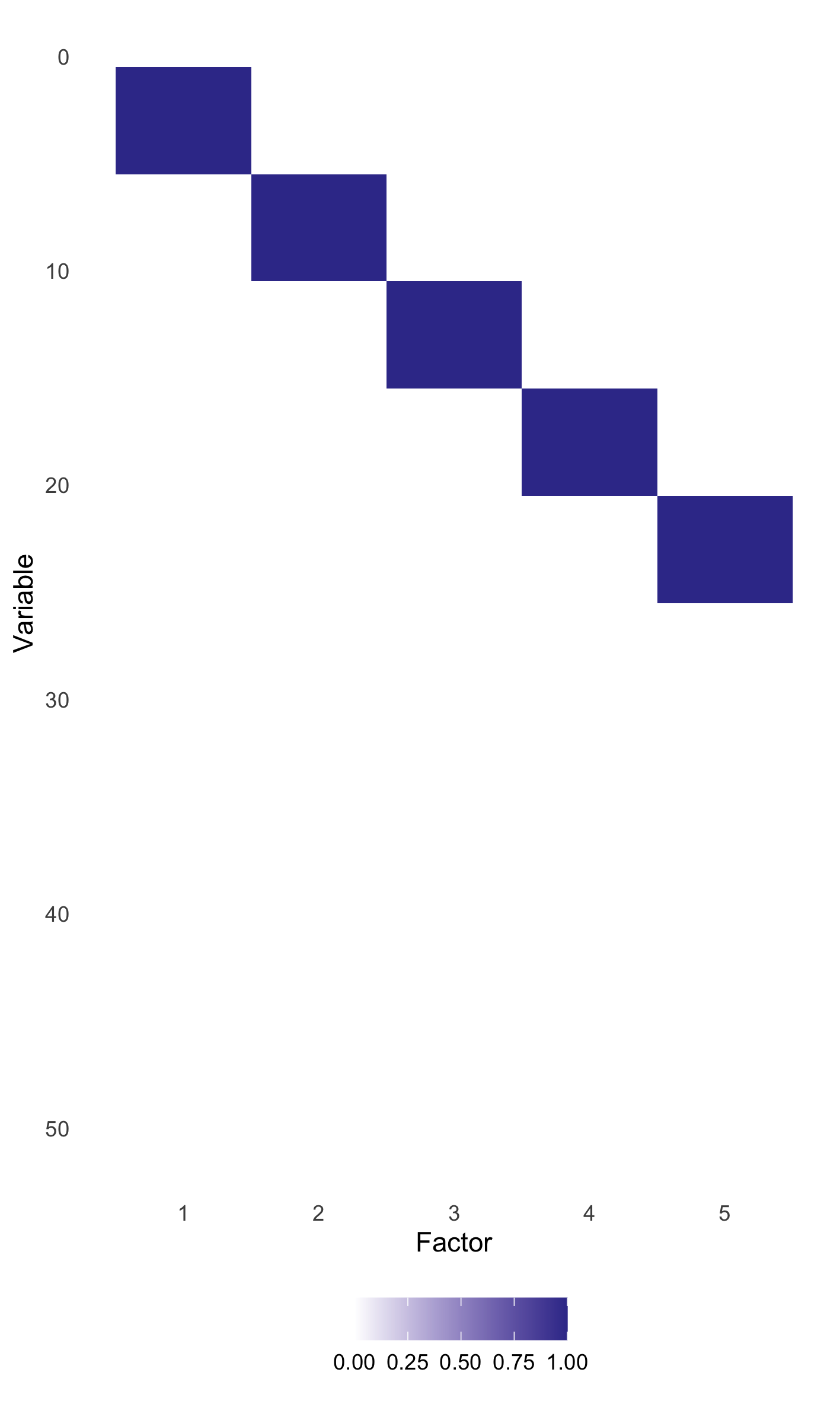
(a) True

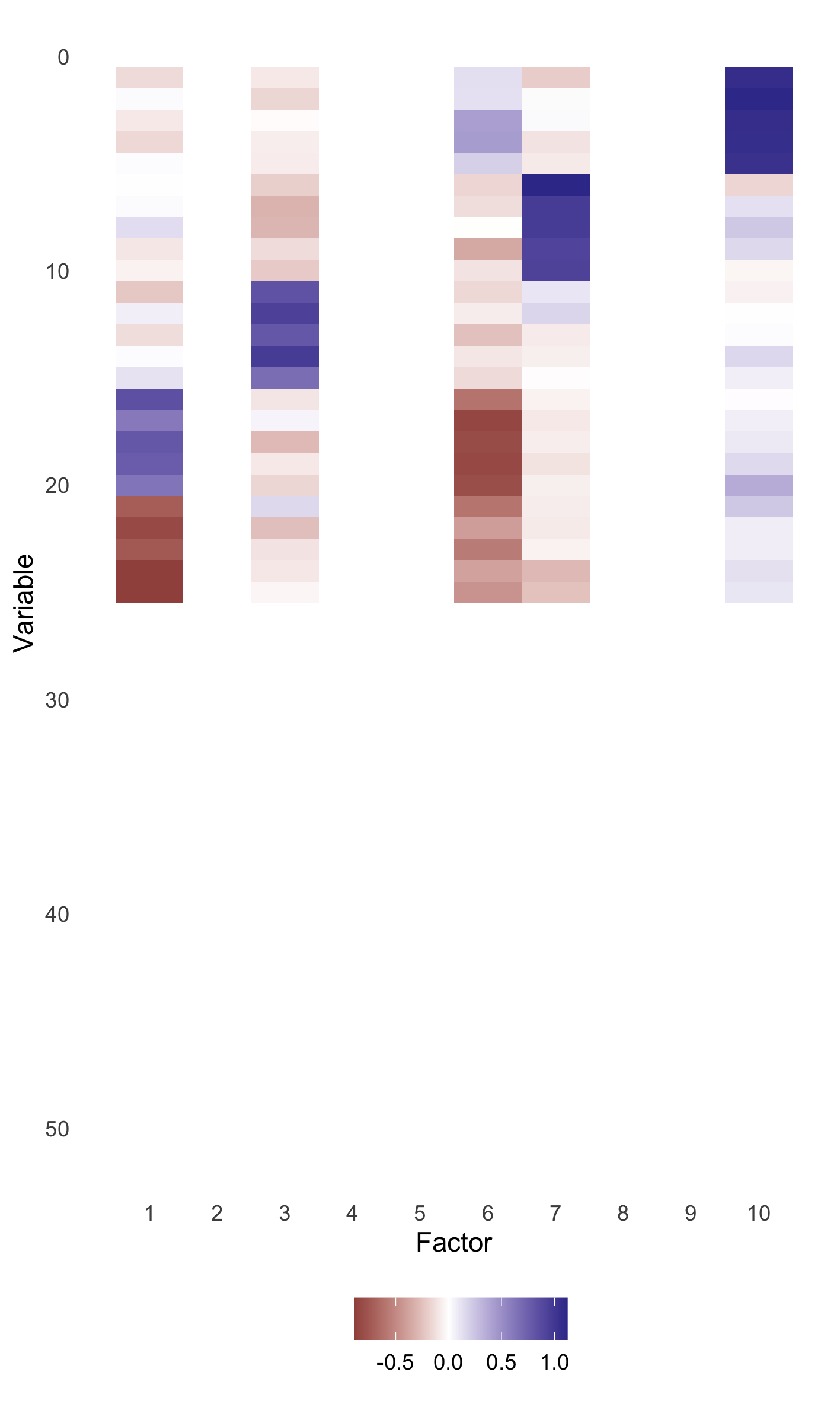
(b) Raw

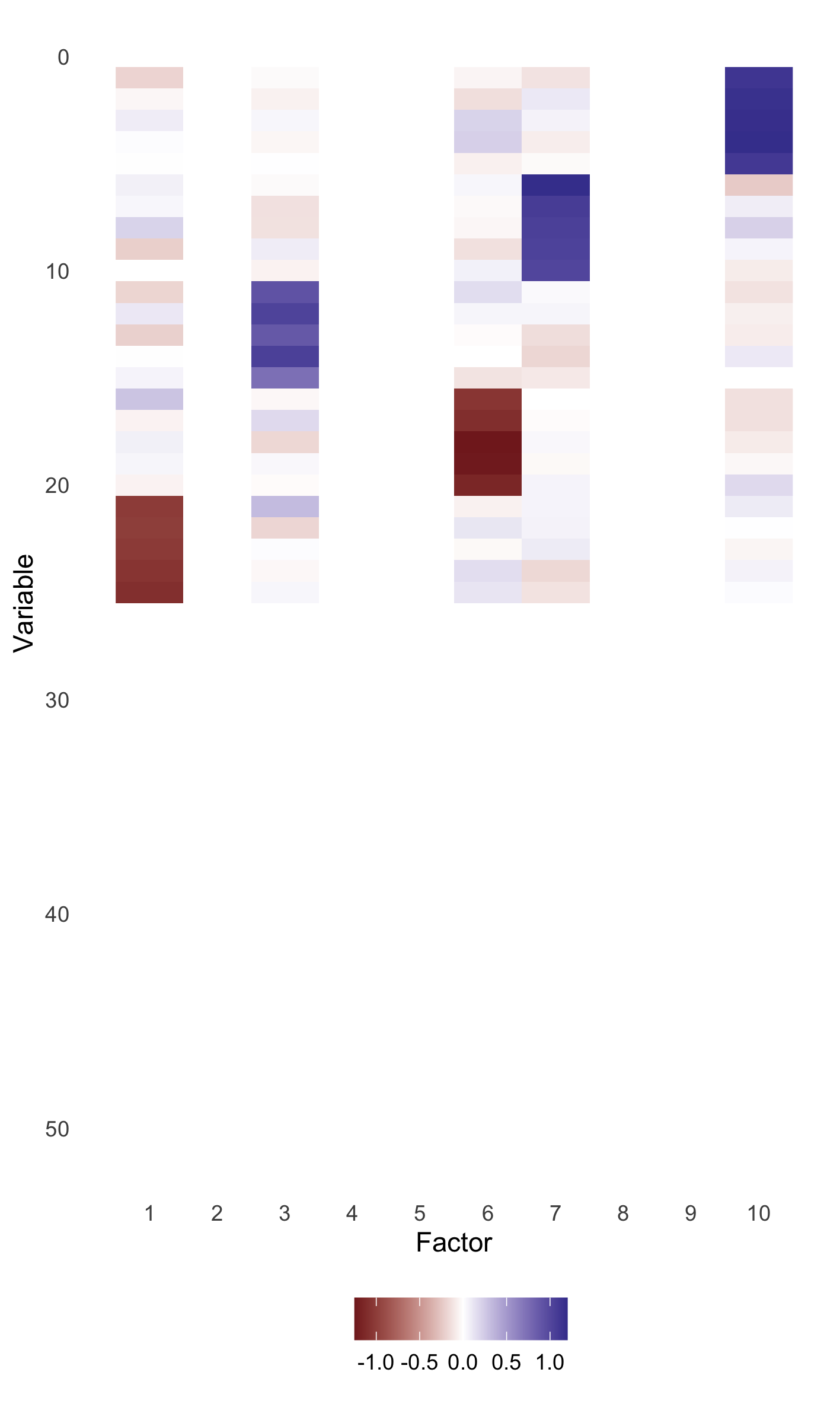
(c) Post-processed

Figure 4: The true pattern of nonzero values in the loading matrix (a), the posterior means of the loading matrix without post-processing (b) and with post-processing (c).

C.3 Sensitivity analysis of the choice of $q$

In this section, we conduct a sensitivity analysis regarding to the choice $q$. The setup for the synthetic dataset is the same as that in the Section 4.1. We only consider the case where the sparsity $s=30$ for simplicity. We compare the posterior distributions of the factor dimensionality $\xi$ for the three values of $q\in\{10,20,50\}$. Figure 5 presents the trace plots of the factor dimensionality. In every case, the trace of the factor dimensionality converges to the true value regardless of the choice of $q$, which suggests that the posterior distribution is insensitive to the choice of $q$.

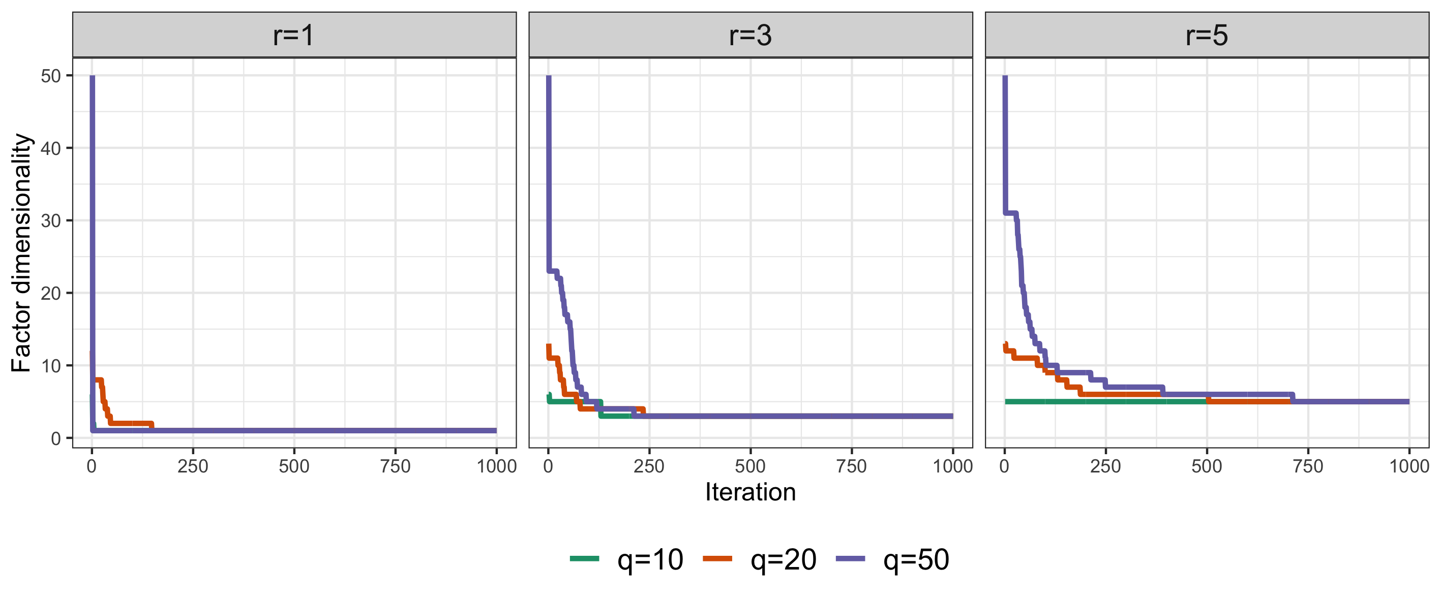
Figure 5: The trace plots of the factor dimensionality for the three values of $q\in\{10,20,50\}$.

C.4 Simulation for large samples

In this section, we conduct a simulation study with synthetic data with $n=500>p=300$. The setup for generating the $s$-sparse true loading matrix $\mathbf{B}^{\star}\in\mathbb{R}^{p\times r}$ is the same as that in the Section 4.1. We let the sparsity $s$ and factor dimensionality $r$ vary among $s\in\{10,30,50\}$ and $r\in\{1,3,5\}$, respectively. Tables 6 and 7 present the simulation results for the factor dimensionality and covariance matrix estimation, respectively, which show that the AdaSS performs well.

Table 6: Proportions of correct estimation (“True”), overestimation (“Over”) and underestimation (“Under”) of the estimated factor dimensionalities for various sparsity $s$ and true factor dimensionality $r$ obtained on 100 synthetic data sets with $n=500$ and $p=300$. “Ave” is the average of the estimated factor dimensionalities.

$s$	$r$		ET	ER	GR	ACT	DT	AdaSS
10	1	True	83	100	100	94	100	100
		Over	17	0	0	6	0	0
		Under	0	0	0	0	0	0
		Ave	1.19	1	1	1.06	1	1
	3	True	96	73	74	25	81	97
		Over	3	0	0	1	0	2
		Under	1	27	26	74	19	1
		Ave	3.02	2.69	2.71	2.25	2.81	3.01
	5	True	91	28	29	0	22	78
		Over	0	0	0	0	0	15
		Under	9	72	71	100	78	7
		Ave	4.9	3.76	3.86	2.05	4.09	5.1
30	1	True	80	100	100	97	100	100
		Over	20	0	0	3	0	0
		Under	0	0	0	0	0	0
		Ave	1.23	1	1	1.03	1	1
	3	True	98	99	99	94	80	100
		Over	2	0	0	6	0	0
		Under	0	1	1	0	20	0
		Ave	3.02	2.99	2.99	3.06	2.8	3
	5	True	100	97	97	86	21	96
		Over	0	0	0	0	0	2
		Under	0	3	3	14	79	2
		Ave	5	4.97	4.97	4.86	4.12	5
50	1	True	78	100	100	98	100	100
		Over	22	0	0	2	0	0
		Under	0	0	0	0	0	0
		Ave	1.26	1	1	1.02	1	1
	3	True	99	100	100	91	0	98
		Over	1	0	0	9	0	0
		Under	0	0	0	0	100	2
		Ave	3.01	3	3	3.09	1.12	2.98
	5	True	100	100	100	100	0	97
		Over	0	0	0	0	0	1
		Under	0	0	0	0	100	2
		Ave	5	5	5	5	3.23	4.99

Table 7: The averages and standard errors of the scaled spectral norm losses of the estimators of the covariance matrix obtained on 100 synthetic data sets with $n=500$ and $p=300$.

$s$	$r$	POET	SPCA-VI	MGPS	MDP	SSL-IBP	ABayes
10	1	0.43 (0.046)	0.084 (0.026)	3.451 (1.311)	0.343 (0.033)	0.238 (0.022)	0.087 (0.029)
	3	0.35 (0.049)	0.114 (0.035)	1.683 (1.173)	0.292 (0.039)	0.218 (0.03)	0.1 (0.029)
	5	0.316 (0.053)	0.132 (0.044)	0.94 (0.614)	0.275 (0.045)	0.227 (0.035)	0.125 (0.044)
30	1	0.432 (0.046)	0.119 (0.036)	5.511 (2.464)	0.342 (0.035)	0.25 (0.032)	0.131 (0.039)
	3	0.41 (0.044)	0.223 (0.049)	3.73 (1.341)	0.33 (0.037)	0.243 (0.024)	0.164 (0.081)
	5	0.379 (0.04)	0.217 (0.034)	2.83 (1.931)	0.314 (0.034)	0.247 (0.026)	0.18 (0.042)
50	1	0.442 (0.047)	0.166 (0.036)	5.003 (2.097)	0.348 (0.036)	0.264 (0.029)	0.178 (0.046)
	3	0.416 (0.044)	0.298 (0.054)	4.346 (1.849)	0.333 (0.037)	0.266 (0.029)	0.201 (0.042)
	5	0.412 (0.039)	0.284 (0.036)	3.799 (2.776)	0.338 (0.035)	0.258 (0.024)	0.248 (0.087)

References

• Ahn and Horenstein [2013] Seung C Ahn and Alex R Horenstein. Eigenvalue ratio test for the number of factors. Econometrica, 81(3):1203–1227, 2013.
• Aßmann et al. [2016] Christian Aßmann, Jens Boysen-Hogrefe, and Markus Pape. Bayesian analysis of static and dynamic factor models: An ex-post approach towards the rotation problem. Journal of Econometrics, 192(1):190–206, 2016.
• Bai and Ng [2002] Jushan Bai and Serena Ng. Determining the number of factors in approximate factor models. Econometrica, 70(1):191–221, 2002.
• Bai and Ng [2006] Jushan Bai and Serena Ng. Confidence intervals for diffusion index forecasts and inference for factor-augmented regressions. Econometrica, 74(4):1133–1150, 2006.
• Bai and Ng [2007] Jushan Bai and Serena Ng. Determining the number of primitive shocks in factor models. Journal of Business & Economic Statistics, 25(1):52–60, 2007.
• Bhattacharya and Dunson [2011] Anirban Bhattacharya and David B Dunson. Sparse Bayesian infinite factor models. Biometrika, 98(2):291–306, 2011.
• Bühlmann and Van De Geer [2011] Peter Bühlmann and Sara Van De Geer. Statistics for high-dimensional data: methods, theory and applications. Springer Science & Business Media, 2011.
• Cai et al. [2013] Tony Cai, Zongming Ma, and Yihong Wu. Sparse PCA: Optimal rates and adaptive estimation. The Annals of Statistics, 41(6):3074–3110, 2013.
• Cai et al. [2015] Tony Cai, Zongming Ma, and Yihong Wu. Optimal estimation and rank detection for sparse spiked covariance matrices. Probability Theory and Related Fields, 161(3-4):781–815, 2015.
• Caprara et al. [1993] Gian Vittorio Caprara, Claudio Barbaranelli, Laura Borgogni, and Marco Perugini. The “big five questionnaire”: A new questionnaire to assess the five factor model. Personality and individual Differences, 15(3):281–288, 1993.
• Carvalho et al. [2008] Carlos M Carvalho, Jeffrey Chang, Joseph E Lucas, Joseph R Nevins, Quanli Wang, and Mike West. High-dimensional sparse factor modeling: applications in gene expression genomics. Journal of the American Statistical Association, 103(484):1438–1456, 2008.
• Chen et al. [2010] Bo Chen, Minhua Chen, John Paisley, Aimee Zaas, Christopher Woods, Geoffrey S Ginsburg, Alfred Hero, Joseph Lucas, David Dunson, and Lawrence Carin. Bayesian inference of the number of factors in gene-expression analysis: application to human virus challenge studies. BMC bioinformatics, 11(1):552, 2010.
• Fan et al. [2008] Jianqing Fan, Yingying Fan, and Jinchi Lv. High dimensional covariance matrix estimation using a factor model. Journal of Econometrics, 147(1):186–197, 2008.
• Fan et al. [2011] Jianqing Fan, Yuan Liao, and Martina Mincheva. High dimensional covariance matrix estimation in approximate factor models. The Annals of Statistics, 39(6):3320, 2011.
• Fan et al. [2012] Jianqing Fan, Xu Han, and Weijie Gu. Estimating false discovery proportion under arbitrary covariance dependence. Journal of the American Statistical Association, 107(499):1019–1035, 2012.
• Fan et al. [2013] Jianqing Fan, Yuan Liao, and Martina Mincheva. Large covariance estimation by thresholding principal orthogonal complements. Journal of the Royal Statistical Society. Series B, Statistical methodology, 75(4), 2013.
• Fan et al. [2017] Jianqing Fan, Lingzhou Xue, and Jiawei Yao. Sufficient forecasting using factor models. Journal of Econometrics, 201(2):292–306, 2017.
• Fan et al. [2018a] Jianqing Fan, Yuan Ke, Qiang Sun, and Wen-Xin Zhou. Farmtest: Factor-adjusted robust multiple testing with approximate false discovery control. Journal of the American Statistical Association, to appear, 2018a.
• Fan et al. [2018b] Jianqing Fan, Han Liu, and Weichen Wang. Large covariance estimation through elliptical factor models. The Annals of Statistics, 46(4):1383, 2018b.
• Fan et al. [2020] Jianqing Fan, Jianhua Guo, and Shurong Zheng. Estimating number of factors by adjusted eigenvalues thresholding. Journal of the American Statistical Association, to appear, 2020.
• Gao and Zhou [2015] Chao Gao and Harrison H Zhou. Rate-optimal posterior contraction for sparse PCA. The Annals of Statistics, 43(2):785–818, 2015.
• Ghosh and Dunson [2009] Joyee Ghosh and David B Dunson. Default prior distributions and efficient posterior computation in bayesian factor analysis. Journal of Computational and Graphical Statistics, 18(2):306–320, 2009.
• Kneip and Sarda [2011] Alois Kneip and Pascal Sarda. Factor models and variable selection in high-dimensional regression analysis. The Annals of Statistics, 39(5):2410–2447, 2011.
• Knowles and Ghahramani [2011] David Knowles and Zoubin Ghahramani. Nonparametric bayesian sparse factor models with application to gene expression modeling. The Annals of Applied Statistics, pages 1534–1552, 2011.
• Lam and Yao [2012] Clifford Lam and Qiwei Yao. Factor modeling for high-dimensional time series: inference for the number of factors. The Annals of Statistics, 40(2):694–726, 2012.
• Latala [2005] Rafal Latala. Some estimates of norms of random matrices. Proceedings of the American Mathematical Society, 133(5):1273–1282, 2005.
• Leek and Storey [2008] Jeffrey T Leek and John D Storey. A general framework for multiple testing dependence. Proceedings of the National Academy of Sciences, 105(48):18718–18723, 2008.
• Leung and Drton [2016] Dennis Leung and Mathias Drton. Order-invariant prior specification in bayesian factor analysis. Statistics & Probability Letters, 111:60–66, 2016.
• Lopes and West [2004] Hedibert Freitas Lopes and Mike West. Bayesian model assessment in factor analysis. Statistica Sinica, pages 41–67, 2004.
• Man and Culpepper [2022] Albert Xingyi Man and Steven Andrew Culpepper. A mode-jumping algorithm for bayesian factor analysis. Journal of the American Statistical Association, 117(537):277–290, 2022.
• Murray et al. [2013] Jared S Murray, David B Dunson, Lawrence Carin, and Joseph E Lucas. Bayesian gaussian copula factor models for mixed data. Journal of the American Statistical Association, 108(502):656–665, 2013.
• Ning [2021] Bo Ning. Spike and slab bayesian sparse principal component analysis. arXiv preprint arXiv:2102.00305, 2021.
• Ohn and Kim [2022] Ilsang Ohn and Yongdai Kim. Posterior consistency of factor dimensionality in high-dimensional sparse factor models. Bayesian Analysis, 17(2):491–514, 2022.
• Onatski [2010] Alexei Onatski. Determining the number of factors from empirical distribution of eigenvalues. The Review of Economics and Statistics, 92(4):1004–1016, 2010.
• Papastamoulis and Ntzoufras [2022] Panagiotis Papastamoulis and Ioannis Ntzoufras. On the identifiability of bayesian factor analytic models. Statistics and Computing, 32(2):23, 2022.
• Pati et al. [2014] Debdeep Pati, Anirban Bhattacharya, Natesh S Pillai, and David Dunson. Posterior contraction in sparse bayesian factor models for massive covariance matrices. The Annals of Statistics, 42(3):1102–1130, 2014.
• Perry and Owen [2010] Patrick O Perry and Art B Owen. A rotation test to verify latent structure. Journal of Machine Learning Research, 11(2), 2010.
• Rockova and George [2016] Veronika Rockova and Edward I George. Fast bayesian factor analysis via automatic rotations to sparsity. Journal of the American Statistical Association, 111(516):1608–1622, 2016.
• Silva [2011] A Pedro Duarte Silva. Two-group classification with high-dimensional correlated data: A factor model approach. Computational Statistics & Data Analysis, 55(11):2975–2990, 2011.
• Srivastava et al. [2017] Sanvesh Srivastava, Barbara E Engelhardt, and David B Dunson. Expandable factor analysis. Biometrika, 104(3):649–663, 2017.
• Stock and Watson [2002] James H Stock and Mark W Watson. Forecasting using principal components from a large number of predictors. Journal of the American Statistical Association, 97(460):1167–1179, 2002.
• Tsybakov [2008] Alexandre B Tsybakov. Introduction to nonparametric estimation. Springer Science & Business Media, 2008.
• Xie et al. [2022] Fangzheng Xie, Joshua Cape, Carey E Priebe, and Yanxun Xu. Bayesian sparse spiked covariance model with a continuous matrix shrinkage prior. Bayesian Analysis, 17(4):1193–1217, 2022.
• Zahn et al. [2007] Jacob M Zahn, Suresh Poosala, Art B Owen, Donald K Ingram, Ana Lustig, Arnell Carter, Ashani T Weeraratna, Dennis D Taub, Myriam Gorospe, Krystyna Mazan-Mamczarz, et al. Agemap: a gene expression database for aging in mice. PLoS Genet, 3(11):e201, 2007.
Supplement to “A Bayesian sparse factor model with adaptive posterior concentration”
Ilsang Ohn, Lizhen Lin and Yongdai Kim