Deep Predictive Coding with Bi-directional Propagation for Classification and Reconstruction

Abstract

This paper presents a new learning algorithm, termed Deep Bi-directional Predictive Coding (DBPC) that allows developing networks to simultaneously perform classification and reconstruction tasks using the same weights. Predictive Coding (PC) has emerged as a prominent theory underlying information processing in the brain. The general concept for learning in PC is that each layer learns to predict the activities of neurons in the previous layer which enables local computation of error and in-parallel learning across layers. In this paper, we extend existing PC approaches by developing a network which supports both feedforward and feedback propagation of information. Each layer in the networks trained using DBPC learn to predict the activities of neurons in the previous and next layer which allows the network to simultaneously perform classification and reconstruction tasks using feedforward and feedback propagation, respectively. DBPC also relies on locally available information for learning, thus enabling in-parallel learning across all layers in the network. The proposed approach has been developed for training both, fully connected networks and convolutional neural networks. The performance of DBPC has been evaluated on both, classification and reconstruction tasks using the MNIST and FashionMNIST datasets. The classification and the reconstruction performance of networks trained using DBPC is similar to other approaches used for comparison but DBPC uses a significantly smaller network. Further, the significant benefit of DBPC is its ability to achieve this performance using locally available information and in-parallel learning mechanisms which results in an efficient training protocol. This results clearly indicate that DBPC is a much more efficient approach for developing networks that can simultaneously perform both classification and reconstruction.

I Introduction

Deep neural networks (DNN) such as AlexNet [1], GoogLeNet [2], VGG [3], and ResNet [4], have performed well on computer vision tasks. These performance benchmarks have been achieved using deeper and wider networks with a large number of parameters which also lead to high computational requirements [5, 6]. Widespread use of edge devices (like mobile phones and drones) has created a necessity for the development of computationally efficient techniques [7, 8] as limited computing available on these devices impedes the deployment of computationally intensive DNNs. Further, most existing DNNs are trained using error-backpropagation (EBP) [9, 10] which relies on sequential layer-wise transmission of information from the last to first layer in the network during training. This is termed as the weight transport problem [11] and severely affects the efficiency of hardware realizations of EBP [12].

Different from EBP, most forms of plasticity observed in the brain rely on locally available information on a synapse which circumvents the weight transport problem. Local learning techniques also create opportunities for parallelizing learning across deep networks with many layers [13, 14]. This has motivated researchers to utilize biological phenomena for developing alternative learning techniques. Predictive coding (PC) [15] has been proposed as a theoretical model of information processing in the brain. PC utilizes locally available information for learning [13, 14, 16] which enables parallelization parameter updates across all layers in the network [13].

The seminal work of Rao and Ballard [15] developed a neural network based implementation of PC that reproduced various phenomena observed in the visual cortex of the brain. The underlying principle of PC is to build generative models by estimating representations that are capable of reconstructing a given input. Each layer in the network generates predictions about representations associated with the previous layers. PC utilizes the gradient of errors in these predictions to update both representations associated with a given layer and the weights in the network. Both representations and weights are updated in parallel across all layers of the network.

It has also been shown that the representations inferred using PC are also suitable for classification [17, 18]. This has led to the development of PC based approaches that involve training a single DNN to perform both discriminative tasks like classification and generative tasks like reconstructing an input [18]. Such techniques are particularly beneficial for edge devices as a single network could perform multiple tasks simultaneously. However, most existing algorithms involving PC have utilized locally available information to update the weights for either image classification [19, 20] or reconstruction [21] but not both at the same time.

In this paper, we develop a new method called Deep Bi-directional Predictive Coding (DBPC) which can be used to build networks that can simultaneously perform classification and reconstruct a given input. The networks trained using DBPC are referred to as Deep Bi-directional Predictive Coding Networks (DBPCNs). The synapses in a DBPCN allow both feedforward and feedback propagation of information using the same weights. This is in contrast to existing studies on PC which only allow feedback propagation to transmit predictions and the errors in these predictions are used to update representations and weights [15]. In DBPCN, each layer simultaneously predicts the activities of neurons in both, previous layer using feedback propagation and next layer using feedforward propagation. The errors in these predictions are used to estimate representations associated with each layer and the weights in the network. Once trained, feedforward propagation from the input to output layer is used for classification. Feedback propagation is used to reconstruct a given input based on representations associated with any given layer in a DBPCN.

The DBPC has been implemented in this paper for networks with both fully connected (DBPC-FCN) and convolutional layers (DBPC-CNN). The performance of these networks has been evaluated using MNIST and FashionMNIST datasets for both classification and reconstruction. The classification accuracy and the images reconstructed using DBPC-FCN and DBPC-CNN are similar to the existing best performing algorithms. For both types of problems, network trained using DBPC require fewer parameters and utilize local learning rules which support parallel learning across all layers in the network.

The rest of the paper is organized as follows. Section II summarizes other approaches in literature that simultaneously perform classification and reconstruction. The architecture of DBPCN and its learning algorithm are presented in Section III. Experimental results using DBPCN are presented in Section IV. Finally, Section V summarizes the conclusions from this study and identifies directions for the future.

II Related work

Over the last few decades, PC has emerged as an important theory of information processing in the brain [22, 23]. Due to a lack of supervisory signal in the brain, most computational studies involving PC in neuroscience develop generative models using unsupervised forms of learning [24, 25]. These studies clamp the activity associated with the input layer while neural activity in other layers is updated to estimate suitable representations. The layer representations estimated using these methods can be used to reconstruct the original input. In [21], PC is further developed and used to train convolutional neural networks for image denoising on Color-MNIST and CIFAR-10.

Several recent studies have developed supervised forms of PC [18, 19, 20]. The key idea in these studies is to clamp activities associated with both, input and output layers to samples and corresponding labels, respectively during training. For testing, only the activity associated with the input layer is clamped to a given sample and the estimated output layer representations are utilized to predict class labels. The networks developed in the above-mentioned studies are only suitable for classification. In [20], PC is used to develop a network that simultaneously performs classification and reconstruction. However, this paper utilizes separate set of parameters in each layer for classification and reconstruction which increases its computational requirements.

In [26], PC is used to develop networks that can simultaneously perform classification and reconstruction using the same set of parameters. PC is only used to estimate the representations associated with each layer. The weights in the network are updated using EBP which relies on non-local information to update the weights and is unsuitable for parallel learning across all layers.

This paper aims to develop a new method to develop networks that can simultaneously perform classification and reconstruction using the same connections. The representations and weights in the proposed method are learned using locally available information to support parallelization of learning across the network.

III Deep Bi-directional Predictive Coding (DBPC)

DBPC can be used for networks with fully connected layers and convolutional neural networks. Here we describe 1) the computations for bi-directional propagation of information in DBPC using a Fully Connected Network (DBPC-FCN); 2) the learning algorithm for estimating representations and updating the weights in DBPC-FCN; and 3) a network architecture for using DBPC to train convolutional neural networks (DBPC-CNN).

III-A Network Architecture

Fig. 1 shows the architecture of the Deep Bi-directional Predictive Coding Fully Connected Network (DBPC-FCN) with $L$ layers. $\mathbf{y}_{l}$ is a vector of shape ($n_{l}\times 1$) which represents the activity of neurons in the $l^{th}$ layer of the network. $n_{l}$ denotes the number of neurons in $l^{th}$ layer. DBPC-FCN employs bi-directional connections (black lines with arrows at both ends) between all layers of the network which enables information to propagate in both, feedforward and feedback directions.

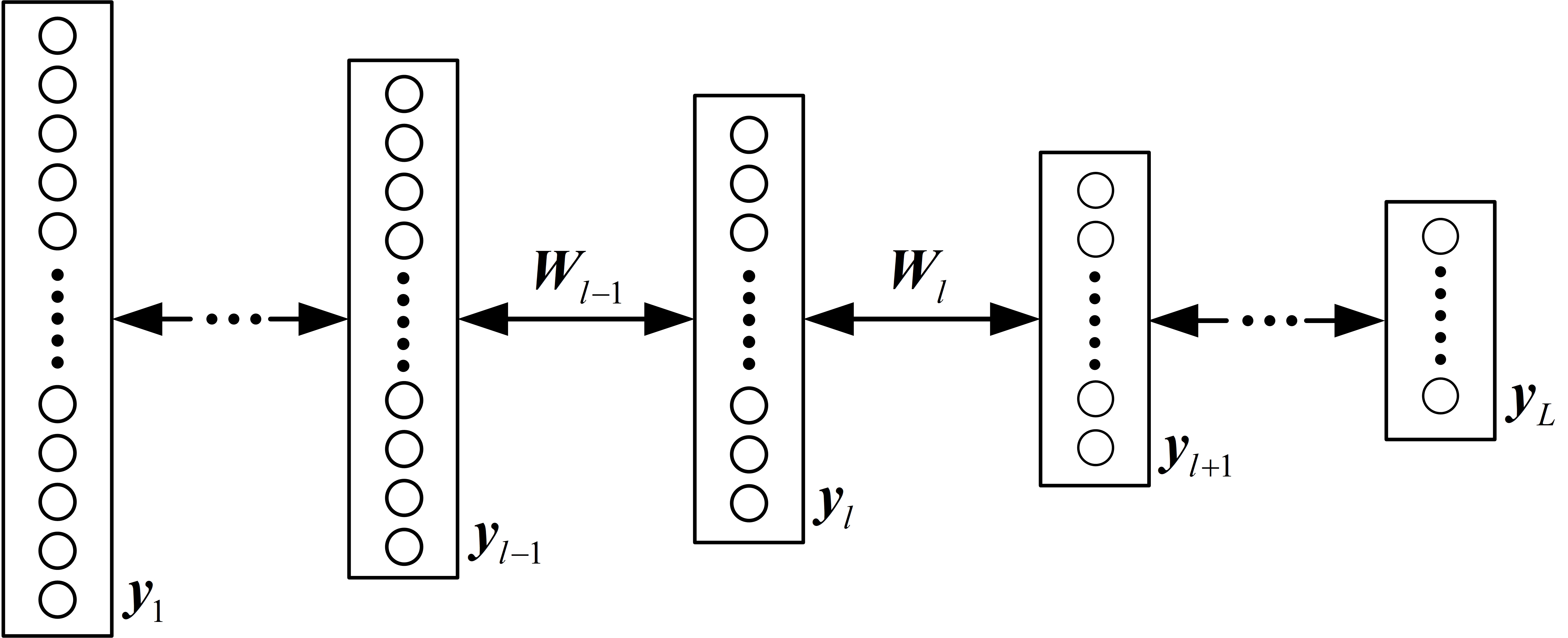
Figure 1: Network architecture of DBPC-FCN with $L$ layers.

Based on feedforward propagation from $(l-1)^{th}$ to $l^{th}$ layer, the activity of neurons in the $l^{th}$ layer is given by

$$\hat{\mathbf{y}}_{l}^{ff}=f(\mathbf{W}_{l-1}\mathbf{y}_{l-1})$$ (1)

where $f$ denotes the activation function and $\mathbf{W}_{l-1}$ is a ($n_{l}\times n_{l-1}$) matrix which denotes the weights of the connections between $(l-1)^{th}$ and $l^{th}$ layer of the network. The Rectified Linear Unit (ReLU) is used as the activation function for all networks in this paper.

Similarly, when feedback propagation is used, the activity of neurons in the $l^{th}$ layer is determined using $(l+1)^{th}$ layer, given by

$$\hat{\mathbf{y}}_{l}^{fb}=f(\mathbf{W}_{l}^{T}\mathbf{y}_{l+1})$$ (2)

where $\mathbf{W}_{l}^{T}$ denotes the transpose of weights $\mathbf{W}_{l}$. Equations (1) and (2) represent the predictions about the activity of neurons in the $l^{th}$ layer based on feedforward propagation from $(l-1)^{th}$ and $(l+1)^{th}$ layer, respectively (see Section III.$B$ for further explanation). It should be noted that both, feedforward and feedback propagation employ the same set of weights.

While training the network an input sample is processed using both, feedforward and feedback propagation. During inference, feedforward propagation is utilized for classification tasks and feedback propagation is used to infer representations that allow reconstructing a given input. For classification, an input sample is presented through the first layer and the predicted class is determined by propagating information from the first layer to the $L^{th}$ layer. Given an input sample $\left(\mathbf{x}_{k}\right)$ and the associated class label $\left(\mathbf{c}_{k}\right)$, the goal of the learning algorithm is to estimate output layer representations that enable correct classification.

III-B Learning Algorithm

The goal of the DBPC is to estimate representations in all layers that can simultaneously be used for classification and reconstruction. The learning algorithm relies only on the locally available information to simultaneously infer representations and update weights in the network. For the $l^{th}$ layer in the network, locally available information includes activities of neurons in the previous $\left((l-1)^{th}\right)$ and next $\left((l+1)^{th}\right)$ layer, and the weights ($\mathbf{W}_{l-1}$ and $\mathbf{W}_{l}$ ) of the connections between these layers. The fundamental concept underlying the learning algorithm is that each layer in the network aims to predict the activities of neurons in the previous (feedback propagation) and next layer (feedforward propagation). The errors in these predictions form the basis of inferring suitable representations (representation learning) and updating the weights (model learning). Below, the two steps of the learning algorithm namely, representation learning and model learning are described in detail.

III-B1 Representation learning

Using feedforward propagation, $l^{th}$ layer in the network receives a prediction of its own neuronal activity from the $(l-1)^{th}$ layer (Equation (1)) and generates a prediction about the activities of neurons in the $(l+1)^{th}$ layer. Based on feedforward propagation, the error $\left(\mathbf{e}_{l-1}^{ff}\right)$ in the prediction about the activity of neurons in the $l^{th}$ layer is given by

$$\mathbf{e}_{l-1}^{ff}=(\mathbf{y}_{l}-\hat{\mathbf{y}}_{l}^{ff})^{2}$$ (3)

Similarly, using feedback propagation, $l^{th}$ layer in the network receives a prediction (Equation (2)) of its own activities from the $(l+1)^{th}$ layer and generates a prediction about the activities of neurons in the $(l-1)^{th}$ layer. Based on feedback propagation, the error $\left(\mathbf{e}_{l}^{fb}\right)$ in the prediction about the activity of neurons in the $l^{th}$ layer is given by

$$\mathbf{e}_{l}^{fb}=(\mathbf{y}_{l}-\hat{\mathbf{y}}_{l}^{fb})^{2}$$ (4)

Figure 2 shows a visualization for computation of all locally computed errors that involve representations $\left(\mathbf{y}_{l}\right)$ associated with $l^{th}$ layer in the network. $\mathbf{y}_{l}$ is updated by performing gradient descent on all the locally computed errors, given by

$$\mathbf{E}_{y_{l}}=\lambda_{f}(\mathbf{e}_{l-1}^{ff}+\mathbf{e}_{l}^{ff})+\lambda_{b}(\mathbf{e}_{l-1}^{fb}+\mathbf{e}_{l}^{fb})$$ (5)

where $\lambda_{f}$ and $\lambda_{b}$ denote feedforward and feedback factors, respectively. $\lambda_{f}$ controls the impact of errors in feedforward predictions on the updated representations. Similarly, $\lambda_{b}$ determines the influence of errors in feedback predictions on the updated representations.

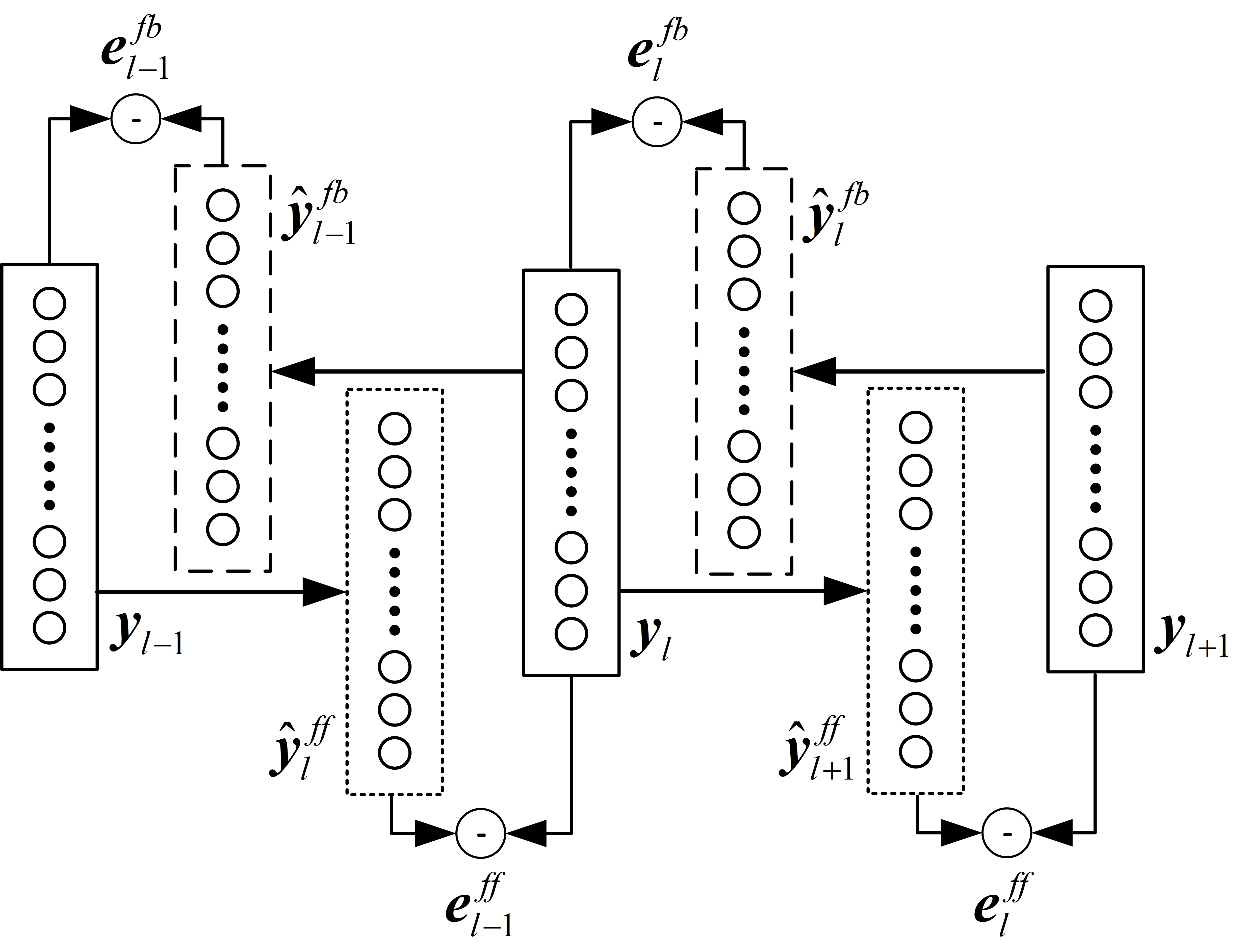
Figure 2: Visualization of the locally computed errors for representation learning and model learning in DBPC. The dotted and dashed rectangles represent the feedforward and feedback predictions, respectively. The circles represent item-wise subtraction required to compute errors in feedforward and feedback predictions.

Minimizing the errors in feedback predictions improves the reconstructions generated by the network and reducing the errors in feedforward predictions improves the classification accuracy of the network. Thus, suitable values for $\lambda_{f}$ and $\lambda_{b}$ help the network to simultaneously perform well on classification and reconstruction tasks.

Based on the error in equation (5), the update $\left(\Delta\mathbf{y}_{l}\right)$ in the representations associated with $l^{th}$ layer are given by

$$\Delta\mathbf{y}_{l}=-\ell_{y}\frac{\delta\mathbf{E}_{y_{l}}}{\delta\mathbf{y}_{l}}$$ (6)

where $\ell_{y}$ denotes the learning rate for updating representation. The representations are updated using the Equations (1)-(6) multiple times as in the original PC algorithm [15]. In this paper, the representations are updated 20 times in DBPC-FCN. Since, all the information required to compute the error in Equations (5) is available locally, the representations for all layers are updated in parallel.

III-B2 Model Learning

The weights in DBPCN are also updated using only locally available information. The weights between $(l-1)^{th}$ and $l^{th}$ layers of the network are updated to minimize the errors in predictions based on feedforward and feedback propagation involving $\mathbf{W}_{l}$. Thus, $\mathbf{W}_{l}$ is updated by performing gradient descent on the errors in Equation (3) and (4), given by

$$\mathbf{E}_{W_{l}}=\beta_{c}\mathbf{e}_{l}^{ff}+\beta_{r}\mathbf{e}_{l}^{fb}$$ (7)

where $\beta_{c}$ and $\beta_{r}$ denote classification and reconstruction factors for updating weights, respectively. $\beta_{c}$ controls the change in weight to improve the feedforward predictions and hence, the classification performance of the DBPCN. Similarly, $\beta_{r}$ determines the change in weight to improve the feedback predictions and hence, the reconstruction performance of the network. Suitable values for $\beta_{c}$ and $\beta_{r}$ enable the network to simultaneously achieve good performance on classification and reconstruction tasks.

Based on the error in equation (7), the change in $\mathbf{W}_{l}$ is given by

$$\Delta\mathbf{W}_{l}=-\ell_{w}\frac{\delta\mathbf{E}_{W_{l}}}{\delta\mathbf{W}_{l}}$$ (8)

where $\ell_{w}$ denotes the learning rate for updating weights. The locally computed error for updating weights ensures that all weights in the network can be updated in parallel. Algorithm 1 presents the pseudocode for the DBPC learning algorithm.

Algorithm 1 Learning algorithm for DBPC

1:Samples and labels {$\mathbf{x}_{k}$, $\mathbf{c}_{k}$}

2:for each epoch do

3:     for each sample do

4:         % Clamp the first and last layer to $\mathbf{x}_{k}$ and $\mathbf{c}_{k}$

5:         $\mathbf{y}_{1}=\mathbf{x}_{k}$,  $\mathbf{y}_{L}=\mathbf{c}_{k}$

6:         % Feedforward propagation

7:         $\hat{\mathbf{y}}_{l}^{ff}=f(\mathbf{W}_{l-1}\mathbf{y}_{l-1})$

8:         % Feedback propagation

9:         $\hat{\mathbf{y}}_{l}^{fb}=f(\mathbf{W}_{l}^{T}\mathbf{y}_{l+1})$

10:         for each iteration do

11:              % Compute errors in Equation 3 and 4

12:              $\mathbf{e}_{l-1}^{ff}=(\mathbf{y}_{l}-\hat{\mathbf{y}}_{l}^{ff})^{2}$

13:              $\mathbf{e}_{l}^{fb}=(\mathbf{y}_{l}-\hat{\mathbf{y}}_{l}^{fb})^{2}$

14:              % Update representation

15:              $\Delta\mathbf{y}_{l}=-\ell_{y}\frac{\delta\mathbf{E}_{y_{l}}}{\delta\mathbf{y}_{l}}$, $\forall l\in[2,\cdots,(L-1)]$

16:         end for

17:         %Update weights

18:         $\Delta\mathbf{W}_{l}=-\ell_{w}\frac{\delta\mathbf{E}_{W_{l}}}{\delta\mathbf{W}_{l}}$, $\forall l\in[1,\cdots,(L-1)]$

19:     end for

20:end for

During testing, only the activities of the neurons in the first layer are clamped to a given input. The activities of neurons in all the other layers of the network are estimated using representation learning. The predicted class is estimated based on the representations associated with the output layer neurons. Further, estimated representations for any other layer can be used to reconstruct the given input using feedback propagation.

III-C DBPC for Convolutional Neural Networks (DBPC-CNN)

We have also developed a network architecture to use DBPC for Convolutional Neural Networks (DBPC-CNN). To enable feedforward and feedback propagation using the same kernels in DBPC-CNN, each layer employs a padding $(P)$, given by

$$P=\frac{K-1}{2}$$ (9)

where $K$ is the size of the kernel and stride in all layers is set to 1. Choosing padding in this way ensures that both input and output for a convolution operation have the same shape. This ensures that convolution operation can be applied in both feedforward and feedback direction using the same kernel.

IV Experiments

This section presents the results of performance evaluation of DBPC for classification and reconstruction tasks. The performance of DBPC is also compared with the other existing algorithms for both tasks. The classification accuracy of DBPC is compared with other PC approaches, namely FIPC₃ [20], PC-1[19] and PCN-E-1 [26]. In addition, the classification accuracy is also compared with the performance of classical DNNs, which include MobileNet-v2 [27] and GoogLeNet [27]. The reconstruction performance of DBPC is compared with the performance of FIPC₃ which is the only other PC approach that is simultaneously capable of classification and reconstruction using representations from any layer in the network.

The performance of DBPC is evaluated in terms of the number of network parameters and accuracy for classification. Given a confusion matrix $Q$, the classification accuracy ($\eta_{c}$) is given by

$$\eta_{c}=\frac{\Sigma_{i\in\{1,\cdots,N_{C}\}}c_{ii}}{\Sigma_{i,j\in\{1,\cdots,N_{C}\}}c_{ij}}$$ (10)

where $c_{ij}$ represents the values in $i^{th}$ row and $j^{th}$ column of the confusion matrix and $N_{C}$ denotes the total number of classes. The Peak Signal-to-Noise Ratio (PSNR) and Structural Similarity Index Measure (SSIM) are used for comparing performance on reconstruction task. The PSNR [28] $(\eta_{r})$ is given by

$$\eta_{r}=10\times\log_{10}\frac{MAX^{2}}{MSE}$$ (11)

where $MAX$ represents the maximum pixel intensity in the image and $MSE$ is the mean squared error between the original image and the reconstructed image. The SSIM [29] $(\eta_{s})$ is given by

$$\eta_{s}(x,y)=\frac{(2\mu_{x}\mu_{y}+C_{1})(2\sigma_{xy}+C_{2})}{(\mu_{x}^{2}+\mu_{y}^{2}+C_{1})(\sigma_{x}^{2}+\sigma_{y}^{2}+C_{2})}$$ (12)

where $x$ and $y$ are the original and the reconstructed images, respectively. $\mu_{x}$ and $\mu_{y}$ represent mean pixel intensity of $x$ and $y$, respectively. $\sigma_{x}$ and $\sigma_{y}$ represent the standard deviations of the pixel intensities in $x$ and $y$, respectively. $\sigma_{xy}$ denotes the covariance of pixel intensities across $x$ and $y$. $C_{1}$ and $C_{2}$ are constants to prevent division by zero.

The performance evaluation is conducted using the MNIST [30] and FashionMNIST [31] datasets. MNIST is a dataset that contains images of hand-written digits from 0 to 9. It has 60,000 grayscale images for training and 10,000 grayscale images for testing. The FashionMNIST dataset is a more challenging dataset that contains images of ten fashion items like T-shirts, trousers and bags. Similar to MNIST, FashionMNIST contains 60,000 grayscale images for training and 10,000 grayscale images for testing. Each image in both datasets is of the size $28\times 28$ pixels.

Table I shows the architectures for DBPC-FCN and DBPC-CNN used for the two datasets. A given row in the table shows details of the corresponding layer in the network. The performance on the MNIST dataset has been evaluated using a fully connected network and a convolutional neural network. For the FashionMNIST dataset, the performance of DBPC is evaluated using only a convolutional neural network. The number of neurons in each layer of DBPC-FCN has been shown using the prefix ‘FC’. Similarly, the prefix ‘Conv’ is used to specify the number of channels in a particular convolutional layer of DBPC-CNN. All convolutional layers use kernel, padding and stride of 3, 1 and 1, respectively.

TABLE I: Architecture for DBPC-FCN and DBPC-CNN

Dataset	MNIST		FashionMNIST
Architecture	DBPC-FCN	DBPCN-CNN	DBPC-CNN
Input Size	$(28\times 28)$
Number of neurons in a layer	FC-1000	Conv-16	Conv-16
	FC-400	Conv-32	Conv-32
	FC-100	Conv-32	Conv-32
		Conv-48	Conv-48
		Conv-48	Conv-48
			Conv-64
			Conv-64
			Conv-96
			Conv-96
Classification	FC-10
#Parameters	1.225M	0.425M	1.004M

All models presented in this paper have been implemented in PyTorch and trained using an Nvidia V100 GPU. Training data is augmented using random rotation and affine transformations. A minibatch of 32 is used during training and stochastic gradient descent (SGD) is used to optimize the network parameters. The total number of epochs is set to 50 and 100 on MNIST and FashionMNIST datasets, respectively.

IV-A Performance Comparison for Classification

Table II shows the results of performance comparison between DBPC and other existing learning algorithms for classification on the MNIST dataset. Figure 3 shows how the classification accuracy of DBPC-FCN and DBPC-CNN evolves during training for the MNIST dataset.

TABLE II: Performance comparison of DBPC with other methods on the MNIST dataset

Methods	Testing Accuracy $\eta_{c}$ (%)	Parameters
Fully Connected Networks
FIPC3[20]	98.84	2.450M
PC-1[19]	98.00	0.532M
PC-2[18]	98.00	1.672M
DBPC-FCN (Proposed work)	97.67	1.225M
Convolutional Neural Networks
PCN-E-1(tied) [26]	99.57	0.070M
MobileNet-v2[27]	99.43	13.600M
GoogLeNet[27]	99.47	49.700M
DBPC-CNN (Proposed work)	99.33	0.425M

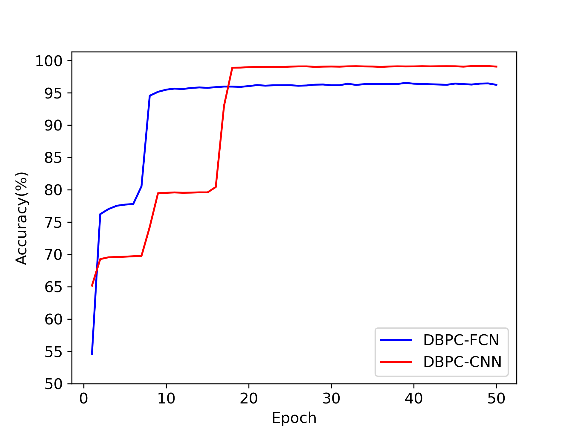
Figure 3: Classification accuracy of DBPC-FCN and DBPC-CNN on MNIST after each epoch of training.

DBPC-FCN uses a network with 1.225 million parameters to achieve a classification accuracy of 97.67% which is 1.2% lower than the best-performing method. FIPC₃ is the best-performing algorithm with an accuracy of 98.84% but it uses twice the number of parameters used by DBPC-FCN. PC-1 uses the smallest network with 0.532 million parameters to achieve an accuracy of 98.00%. It may be noted that representations estimated in both, PC-1 and PC-2 can’t be used for reconstruction whereas DBPC-FCN also supports reconstruction of inputs.

The performance of all the methods used for comparison is better using convolutional neural networks. DBPC-CNN employs a network with 0.425 million parameters to achieve an accuracy of 99.33% which is similar to the performance of other learning algorithms used for comparison. PCN-E-1 (tied) is the best performing algorithm with an accuracy of 99.57% and it uses a network with 0.07 million parameters. It may be noted that PCN-E-1 uses error-backpropagation for training which relies on non-local information for learning and is not suitable for parallel training across layers in the network. DBPC-CNN allows reconstruction of inputs using representations estimated for any layer in the network. The ability of PCN-E-1 to reconstruct images using representations estimated for different layers hasn’t been studied. The performance of DBPC-CNN is also similar to the classification accuracy of established networks like MobileNet-v2 [27] and GoogLeNet [27] which are not capable of reconstruction. Further, DBPC-CNN employs a network that is much smaller than those used by MobileNet-v2 and GoogLeNet.

TABLE III: Performance comparison of DBPC-CNN with PC-1 on the FashionMNIST dataset

Methods	Testing Accuracy $\eta_{c}$ (%)	Parameters
PC-1[19]	89.00	0.532M
DBPC-CNN	91.61	1.004M

Table III shows a performance comparison of DBPC-CNN with other methods on the more challenging FashionMNIST dataset. It may be noted that only DBPC-CNN is used for the FashionMNIST dataset due to the higher complexity of this dataset. Figure 4 shows the changes in the classification accuracy of DBPC-CNN after each epoch of training for the FashionMNIST dataset. DBPC-CNN uses a network with 1.004 million parameters to achieve an accuracy of 91.61%. The performance of DBPC-CNN is 2.9% higher than the classification accuracy of PC-1. Furthermore, as highlighted above, the representations estimated in PC-1 cannot be used for reconstructing the inputs.

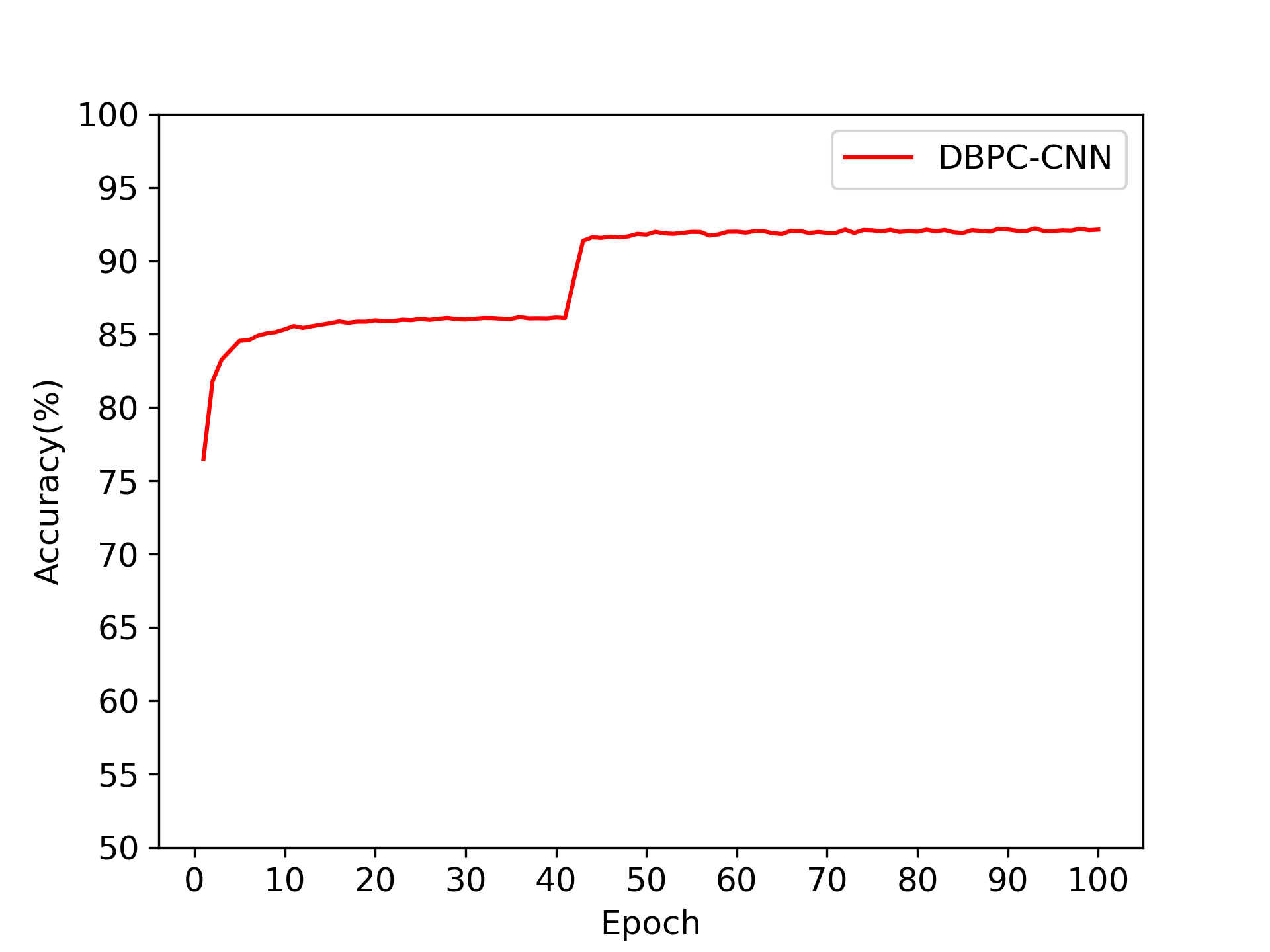
Figure 4: Classification accuracy of DBPC-CNN on FashionMNIST after each epoch of training.

IV-B Performance Comparison for Reconstruction

In this section, the performance of DBPC-FCN and DBPC-CNN is evaluated and compared for reconstruction problems using MNIST and FashionMNIST datasets. Figure 5(a) and 5(b) show how the PSNR of the reconstructed images form each layer in DBPC-FCN and DBPC-CNN evolves during training, respectively. For both DBPC-FCN and DBPC-CNN, earlier layers achieved a higher PSNR compared to deeper layers in the network. Further, reconstructed images obtained using DBPC-CNN exhibited higher PSNR compared to DBPC-FCN. Similar results are also obtained for the SSIM based on reconstructed images obtained from DBPC-FCN and DBPC-CNN.

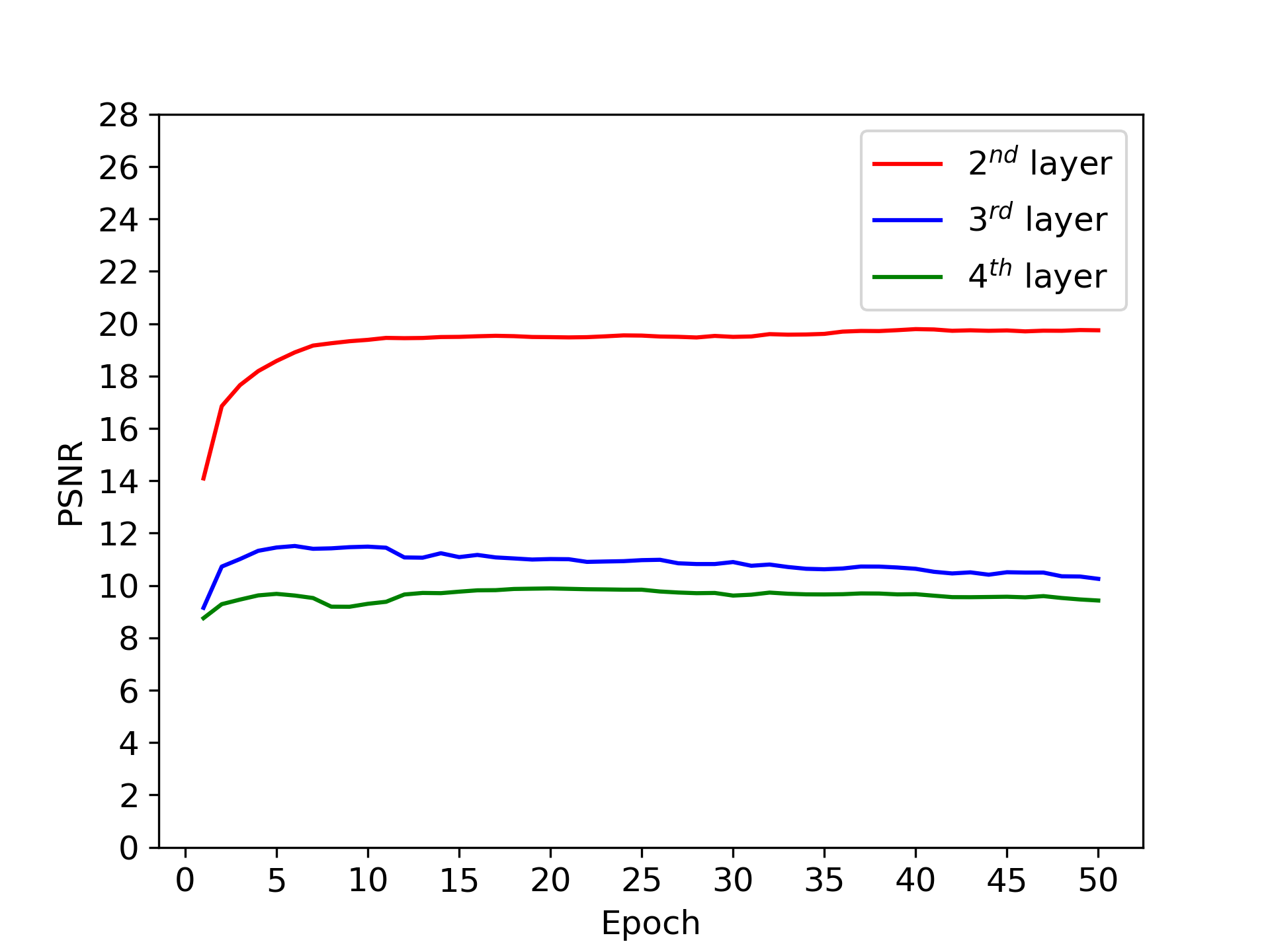
(a) PSNR of DBPC-FCN

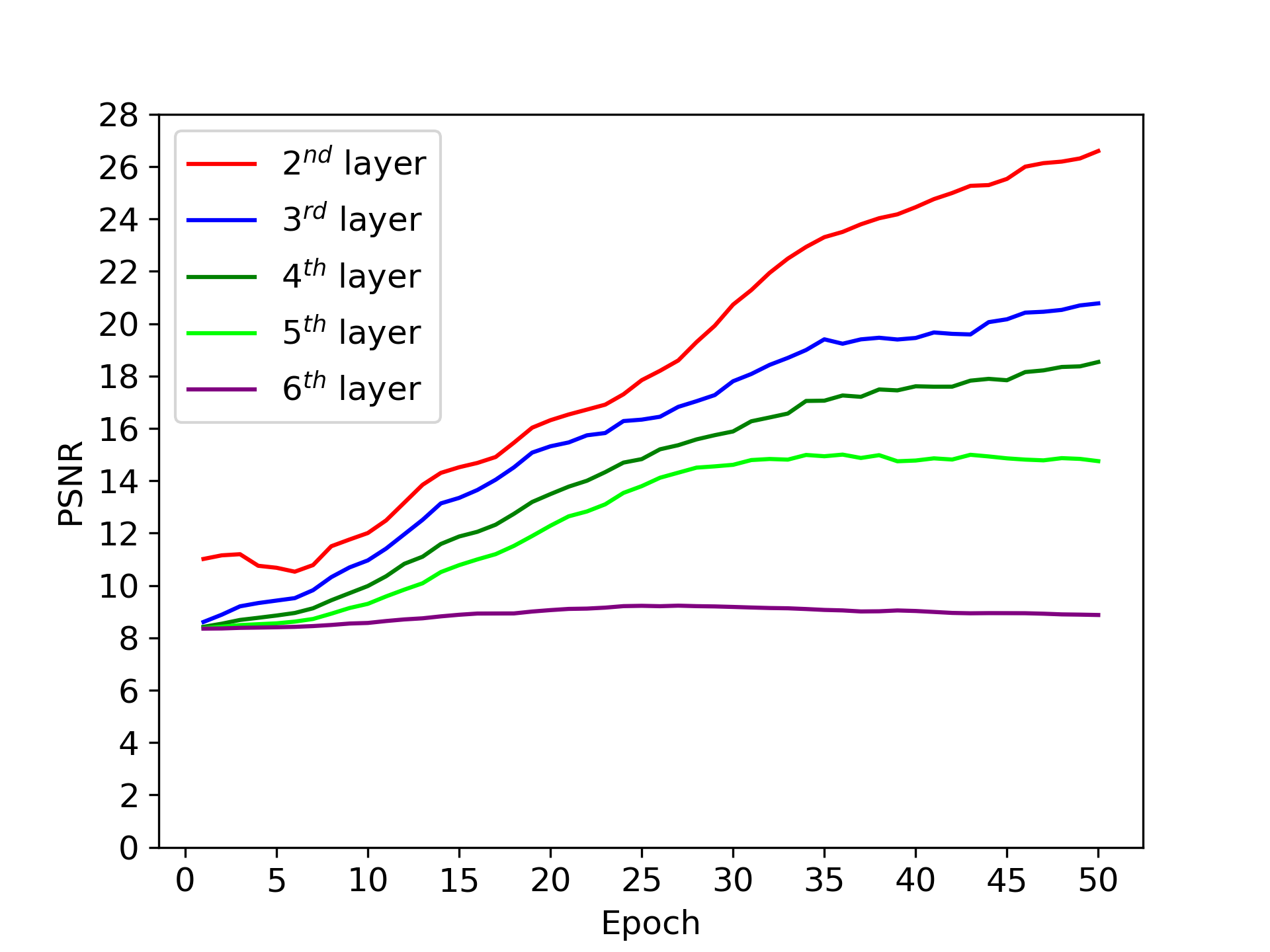
(b) PSNR of DBPC-CNN

Figure 5: PSNR of (a) DBPC-FCN and (b) DBPC-CNN on MNIST after each epoch of training, respectively.

Figure 6 shows the reconstructed images obtained using representations estimated for each layer in FIPC₃, DBPC-FCN and DBPC-CNN. The first column in each figure shows the original figure in the dataset and the following columns show the reconstructions obtained from successively deeper layers in the network. These reconstructions are obtained by propagating backward from a given layer using the representations estimated in that layer. It may be observed that the quality of reconstructed images deteriorates as we go from earlier to deeper layers in all three algorithms. The deterioration in image quality is lowest for DBPC-CNN. It may be noted that FIPC₃ uses a separate set of weights for classification and reconstruction which results in a network having a large number of parameters.

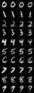
(a) FIPC₃

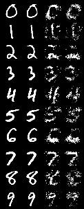
(b) DBPC-FCN

(c) DBPC-CNN

Figure 6: MNIST images reconstructed using (a) FIPC₃, (b) DBPC-FCN and (c) DBPC-CNN, respectively. The first column in each panel represents the original image from the MNIST dataset, and the other columns from left to right display the reconstructions from a given layer in the network.

Figure 7 show the images reconstructed using representations associated with each layer of DBPC-CNN for the FashionMNIST dataset. The layout of Figure 7 and the method used for reconstructing these images is the same as that used for the MNIST dataset. Table IV provides a summary of the results presented above using a quantitative comparison of images reconstructed by DBPC-FCN and DBPC-CNN based on the PSNR and SSIM metric on both datasets.

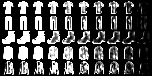
Figure 7: Reconstruction results of DBPC-CNN on FashionMNIST. The first column in each subplot represents the original input image from the test FashMNIST dataset, and the other columns from left to right display the reconstructions from each representation layer.

TABLE IV: Quantitative comparison of images reconstructed by DBPC-FCN and DBPC-CNN based on PSNR and SSIM

Methods	Datasets	$l^{th}$ layer	Testing PSNR ($\eta_{r}$)	Testing SSIM ($\eta_{s}$)
DBPC-FCN	MNIST	$2^{nd}$ layer	20.21	0.9169
		$3^{rd}$ layer	10.29	0.3851
		$4^{th}$ layer	9.45	0.2223
DBPC-CNN		$2^{nd}$ layer	26.90	0.9779
		$3^{rd}$ layer	20.58	0.9228
		$4^{th}$ layer	19.17	0.8967
		$5^{th}$ layer	17.05	0.8304
		$6^{th}$ layer	10.88	0.3832
DBPC-CNN	FashionMNIST	$2^{nd}$ layer	31.12	0.9880
		$3^{rd}$ layer	18.32	0.8353
		$4^{th}$ layer	14.36	0.6572
		$5^{th}$ layer	11.91	0.5719
		$6^{th}$ layer	10.79	0.5228
		$7^{th}$ layer	8.73	0.4246
		$8^{th}$ layer	7.92	0.3805
		$9^{th}$ layer	6.86	0.3208
		$10^{th}$ layer	4.83	0.1228

V Conclusion

In this paper, a new Deep Bi-directional Predictive Coding (DBPC) that supports developing networks that can simultaneously perform classification and reconstruction has been proposed and proven to operate efficiently. The proposed DBPC builds on existing PC methods by developing a network in which each layer simultaneously predicts the activities of neurons in the previous and next layer to simultaneously perform classification and reconstruction tasks. The performance of networks trained using DBPC has been evaluated for classification and reconstruction tasks using the MNIST and FashionMNIST datasets. The results of performance comparison clearly indicate that the classification and reconstruction performance of DBPC is similar to other existing approaches but, DBPC employs a significantly smaller network. In addition, DBPC relies on locally available information for learning and employs in-parallel updates across all layers in the network which results in a more efficient training protocol. Future directions on this work will focus on extending the reconstruction capabilities of DBPC to generate samples in the input space.

References

- [1] A. Krizhevsky, I. Sutskever, and G. E. Hinton, “Imagenet classification with deep convolutional neural networks,” in Advances in Neural Information Processing Systems, F. Pereira, C. Burges, L. Bottou, and K. Weinberger, Eds., vol. 25. Curran Associates, Inc., 2012. [Online]. Available: https://proceedings.neurips.cc/paper/2012/file/c399862d3b9d6b76c8436e924a68c45b-Paper.pdf
- [2] C. Szegedy, W. Liu, Y. Jia, P. Sermanet, S. E. Reed, D. Anguelov, D. Erhan, V. Vanhoucke, and A. Rabinovich, “Going deeper with convolutions,” CoRR, vol. abs/1409.4842, 2014. [Online]. Available: http://arxiv.org/abs/1409.4842
- [3] K. Simonyan and A. Zisserman, “Very deep convolutional networks for large-scale image recognition,” arXiv preprint arXiv:1409.1556, 2014.
- [4] K. He, X. Zhang, S. Ren, and J. Sun, “Deep residual learning for image recognition,” in Proceedings of the IEEE conference on computer vision and pattern recognition, 2016, pp. 770–778.
- [5] J.-P. Lachaux, M. Chavez, and A. Lutz, “A simple measure of correlation across time, frequency and space between continuous brain signals,” Journal of neuroscience methods, vol. 123, no. 2, pp. 175–188, 2003.
- [6] B. Lim and S. Zohren, “Time-series forecasting with deep learning: a survey,” Philosophical Transactions of the Royal Society A, vol. 379, no. 2194, p. 20200209, 2021.
- [7] M. S. Murshed, C. Murphy, D. Hou, N. Khan, G. Ananthanarayanan, and F. Hussain, “Machine learning at the network edge: A survey,” ACM Computing Surveys (CSUR), vol. 54, no. 8, pp. 1–37, 2021.
- [8] V. Saranirad, S. Dora, and D. Coyle, “Dob-snn: A new neuron assembly-inspired spiking neural network for pattern classification,” in 2021 International Joint Conference on Neural Networks (IJCNN). IEEE, 2021, pp. 1–6.
- [9] D. E. Rumelhart, G. E. Hinton, and R. J. Williams, “Learning representations by back-propagating errors,” nature, vol. 323, no. 6088, pp. 533–536, 1986.
- [10] P. J. Werbos, “Applications of advances in nonlinear sensitivity analysis,” in System modeling and optimization. Springer, 1982, pp. 762–770.
- [11] S. Grossberg, “Competitive learning: From interactive activation to adaptive resonance,” Cognitive Science, vol. 11, no. 1, pp. 23–63, 1987. [Online]. Available: https://www.sciencedirect.com/science/article/pii/S0364021387800253
- [12] B. Crafton, M. West, P. Basnet, E. Vogel, and A. Raychowdhury, “Local learning in rram neural networks with sparse direct feedback alignment,” in 2019 IEEE/ACM International Symposium on Low Power Electronics and Design (ISLPED), 2019, pp. 1–6.
- [13] B. Millidge, T. Salvatori, Y. Song, R. Bogacz, and T. Lukasiewicz, “Predictive coding: Towards a future of deep learning beyond backpropagation?” arXiv preprint arXiv:2202.09467, 2022.
- [14] J. C. Whittington and R. Bogacz, “Theories of error back-propagation in the brain,” Trends in cognitive sciences, vol. 23, no. 3, pp. 235–250, 2019.
- [15] R. P. Rao and D. H. Ballard, “Predictive coding in the visual cortex: a functional interpretation of some extra-classical receptive-field effects,” Nature neuroscience, vol. 2, no. 1, pp. 79–87, 1999.
- [16] Y. Song, T. Lukasiewicz, Z. Xu, and R. Bogacz, “Can the brain do backpropagation?—exact implementation of backpropagation in predictive coding networks,” Advances in neural information processing systems, vol. 33, pp. 22 566–22 579, 2020.
- [17] S. Dora, S. M. Bohte, and C. M. Pennartz, “Deep gated hebbian predictive coding accounts for emergence of complex neural response properties along the visual cortical hierarchy,” Frontiers in Computational Neuroscience, vol. 15, p. 666131, 2021.
- [18] W. Sun and J. Orchard, “A predictive-coding network that is both discriminative and generative,” Neural computation, vol. 32, no. 10, pp. 1836–1862, 2020.
- [19] B. Millidge, A. Tschantz, A. Seth, and C. L. Buckley, “Relaxing the constraints on predictive coding models,” arXiv preprint arXiv:2010.01047, 2020.
- [20] Z. Song, J. Zhang, G. Shi, and J. Liu, “Fast inference predictive coding: A novel model for constructing deep neural networks,” IEEE transactions on neural networks and learning systems, vol. 30, no. 4, pp. 1150–1165, 2018.
- [21] A. Ororbia and A. Mali, “Convolutional neural generative coding: Scaling predictive coding to natural images,” arXiv preprint arXiv:2211.12047, 2022.
- [22] D. Mumford, “On the computational architecture of the neocortex: Ii the role of cortico-cortical loops,” Biological cybernetics, vol. 66, no. 3, pp. 241–251, 1992.
- [23] K. Friston, “A theory of cortical responses,” Philosophical transactions of the Royal Society B: Biological sciences, vol. 360, no. 1456, pp. 815–836, 2005.
- [24] M. W. Spratling, “Predictive coding as a model of biased competition in visual attention,” Vision research, vol. 48, no. 12, pp. 1391–1408, 2008.
- [25] ——, “Reconciling predictive coding and biased competition models of cortical function,” Frontiers in computational neuroscience, p. 4, 2008.
- [26] H. Wen, K. Han, J. Shi, Y. Zhang, E. Culurciello, and Z. Liu, “Deep predictive coding network for object recognition,” in International Conference on Machine Learning. PMLR, 2018, pp. 5266–5275.
- [27] L. M. Seng, B. B. C. Chiang, Z. A. A. Salam, G. Y. Tan, and H. T. Chai, “Mnist handwritten digit recognition with different cnn architectures,” Journal of Applied Technology and Innovation (e-ISSN: 2600-7304), vol. 5, no. 1, p. 7, 2021.
- [28] A. Hore and D. Ziou, “Image quality metrics: Psnr vs. ssim,” in 2010 20th international conference on pattern recognition. IEEE, 2010, pp. 2366–2369.
- [29] Z. Wang, A. C. Bovik, H. R. Sheikh, and E. P. Simoncelli, “Image quality assessment: from error visibility to structural similarity,” IEEE transactions on image processing, vol. 13, no. 4, pp. 600–612, 2004.
- [30] Y. LeCun, L. Bottou, Y. Bengio, and P. Haffner, “Gradient-based learning applied to document recognition,” Proceedings of the IEEE, vol. 86, no. 11, pp. 2278–2324, 1998.
- [31] H. Xiao, K. Rasul, and R. Vollgraf, “Fashion-mnist: a novel image dataset for benchmarking machine learning algorithms,” arXiv preprint arXiv:1708.07747, 2017.