Privileged Knowledge Distillation for Sim-to-Real Policy Generalization

Abstract

Reinforcement Learning (RL) has recently achieved remarkable success in robotic control. However, most RL methods operate in simulated environments where privileged knowledge (e.g., dynamics, surroundings, terrains) is readily available. Conversely, in real-world scenarios, robot agents usually rely solely on local states (e.g., proprioceptive feedback of robot joints) to select actions, leading to a significant sim-to-real gap. Existing methods address this gap by either gradually reducing the reliance on privileged knowledge or performing a two-stage policy imitation. However, we argue that these methods are limited in their ability to fully leverage the privileged knowledge, resulting in suboptimal performance. In this paper, we propose a novel single-stage privileged knowledge distillation method called the Historical Information Bottleneck (HIB) to narrow the sim-to-real gap. In particular, HIB learns a privileged knowledge representation from historical trajectories by capturing the underlying changeable dynamic information. Theoretical analysis shows that the learned privileged knowledge representation helps reduce the value discrepancy between the oracle and learned policies. Empirical experiments on both simulated and real-world tasks demonstrate that HIB yields improved generalizability compared to previous methods.

1 Introduction

Reinforcement learning (RL) has achieved remarkable progress and has been applied to various domains, including games, financial trading, and robotics. However, most RL methods work in simulated environments, and their applications in real-world scenarios are still challenging. To obtain an RL policy for the real-world scenario, one way is to interact with the real environment directly. However, since RL method requires a large number of interactions and also needs to handle potentially dangerous behaviors, applying such a method is prohibitive in scenarios where safety is important [13]. A more efficient way is to learn a policy in the simulated environment first and then transfer it to the real-world environment. Nevertheless, there is always an inherent mismatch between the simulated environment and the real environment. Such mismatch makes the policy learned from the simulated environment performs sub-optimally in real-world environment, which is known as a sim-to-real gap [22, 21, 28]. Previous works tackle this problem in the inspects of sensing and actuation, where the sensing mismatch can be alleviated via adversarial training [1, 19] and the actuation mismatch can be minimized by more realistic simulation [33]. Another branch of methods is domain randomization [8, 29], which tackles both mismatches by introducing additional perturbances in the simulator [49]. The intuition behind domain randomization is to cover the real-world environment by randomized environments. However, such randomization assumes that the state spaces of the simulators and that of the real-world scenarios are the same, which is typically not the case. Meanwhile, previous methods neither reconstruct privileged knowledge nor take advantage of history, which we believe are important to close the sim-to-real gap.

To demonstrate the importance of privileged knowledge, we consider a more realistic and challenging sim-to-real setting, where the simulation and real-world environment provide different information. Such a setting is common for real-world robotics applications since the simulated environment often provides the oracle state information, including privileged knowledge (e.g., dynamics, surroundings, terrains), while the real robot can only rely on local states (e.g., proprioceptive feedback of robot joints) to select the action. Such a sim-to-real gap can also be extended to a general policy generalization problem with a knowledge gap. Previous methods solve this problem via a two-stage policy distillation process [34]. In particular, a teacher policy is first trained in the simulator with oracle states, then a student policy with local states is trained by imitating the teacher policy. Nevertheless, such a two-stage paradigm is computationally expensive and requires careful design for imitation. An alternative way is to gradually drop the privileged information as the policy trained [23], which, however, cannot take advantage of the known privileged information sufficiently in training.

In this paper, we present a representation-based approach, instead of policy distillation, to better utilize the privileged knowledge from training data with a single-stage learning paradigm. In particular, we propose a novel method called Historical Information Bottleneck (HIB) to distill the privileged knowledge. HIB takes advantage of historical information that contains previous local states and actions to learn a history representation, which is trained by maximizing the mutual information (MI) between the representation and the privileged knowledge. Theoretically, we show that maximizing such an MI term will minimize the privileged knowledge modeling error, reducing the discrepancy between the optimal value function and the learned value function. Furthermore, motivated by the Information Bottleneck (IB) principle, we compress the decision-irrelevant information from the history and obtain a more robust representation. The IB objective is approximated by variational lower bounds to handle the high-dimensional state space.

In summary, our contributions are threefold: (i) We propose a novel policy generalization method called HIB that follows the Information Bottleneck (IB) [40] principle to distill privileged knowledge from a fixed length of history. (ii) We provide a theoretical analysis of both the policy distillation methods and the proposed method, which shows that minimizing the privilege modeling error is crucial in learning a near-optimal policy. (iii) Empirically, we show that HIB learns robust representation in randomized RL environments and achieves better generalization performance in both simulated and real-world environments than SOTA algorithms, including out-of-distribution test environments.

2 Related Work

Sim-to-Real Transfer. Transferring RL policies from simulation to reality is challenging due to the domain mismatch between the two domains. To this end, the previous study hinges on domain randomization, which trains the policy under a wide range of environmental parameters and sensor noises [50, 6, 30]. However, domain randomization typically sacrifices the optimality for robustness, leading to an over-conservative policy [47]. In addition, domain randomization cannot handle the more challenging setting where the simulator contains privileged knowledge that is unavailable in the real world. To address this problem, policy distillation methods [22, 21, 28] perform privilege distillation by first learning a teacher policy with access to the privileged knowledge, and then using the historical trajectories as inputs to distill a student policy through supervised training. However, policy distillation is sample inefficient and cannot bridge the knowledge gap effectively. An alternative distillation method gradually drops privileged knowledge [23], while it still sacrifices optimality for better generalization and cannot fully leverage historical knowledge. In contrast, our method distill privileged knowledge in a single stage, resulting in better utilization of historical information.

Contrastive Representation. Contrastive representation learning is a class of methods that learn a representation that obeys similarity constraints in a dataset typically organized by similar and dissimilar pairs [44, 16, 7]. Contrastive learning has been recently used in RL as auxiliary tasks to improve sample efficiency. Srinivas et al. [39] combines data augmentation [48] and contrastive loss for image-based RL. Other methods also use contrastive learning to extract dynamics-relevant [26, 32], temporal consistent [38] or goal-conditional [10] information, thereby obtaining a stable and task-relevant representation. In our use case, we select similar pairs by the privileged knowledge obtained and its corresponding trajectory history. Furthermore, we aim to distill the privileged knowledge in a representation space without negative sampling. We highlight that we propose the first representation learning method that learns a privilege representation for policy generalization.

Information Bottleneck for RL. The IB principle [41, 40] was initially proposed to trade off the accuracy and complexity of the representation in supervised learning. Specifically, IB maximizes the MI between representation and targets to extract useful features, while also compressing the irrelevant information by limiting the MI between representation and raw inputs [2, 35]. Recently, IB has been employed in RL to acquire a compact and robust representation. For example, Fan and Li [11] takes advantage of IB to learn task-relevant representation via a multi-view augmentation. Other methods [20, 24, 3] maximize the MI between representation and dynamics or value function, and restrict the information to encourage the encoder to extract only the task-relevant information. Unlike the previous works that neither tackle the policy generalization problem nor utilize historical information, HIB derives a novel objective based on IB, which aims to learn a robust representation of privileged knowledge from history while simultaneously removing redundant decision-irrelevant information.

3 Preliminaries

In this section, we briefly introduce the problem definition and the corresponding notations used throughout this paper. We give the definition of privileged knowledge in robot learning as follows.

Definition 1 (Privileged Knowledge).

Privileged knowledge is the hidden state that is inaccessible in the real environment but can be obtained in the simulator, e.g., surrounding heights, terrain types, and dynamic parameters like fraction and damping. An oracle (teacher) policy is defined as the optimal policy with privileged knowledge visible.

In the policy generalization problem, we define the MDP as $\mathcal{M}=(\mathcal{S}^{l},\mathcal{S}^{p},\mathcal{A},P,r,\mathcal{\gamma})$, where $[s^{l},s^{p}]=s^{o}$ represents the oracle state $s^{o}$ that contains $s^{l}\in\mathcal{S}^{l}$ (i.e., the local state space) and $s^{p}\in\mathcal{S}^{p}$ (i.e., the privileged state space), where $s^{p}$ contains privileged knowledge defined in Definition 1. $\mathcal{A}$ is the action space. The transition function $P(s^{o}_{t+1}|s^{o}_{t},a_{t})$ and reward function $r(s^{o},a)$ follows the ground-truth dynamics based on the oracle states. Based on the MDP, we define two policies: $\pi(a|s^{l},s^{p})$ and $\hat{\pi}(a|s^{l})$, for the simulation and real world, respectively. Specifically, $\pi(a|s^{l},s^{p})$ is an oracle policy that can access the privileged knowledge, which is only accessible in the simulator. In contrast, $\hat{\pi}(a|s^{l})$ is a local policy without accessing the privileged knowledge throughout the interaction process, which is common in the real world.

One could reminisce about Partially Observable MDP (POMDP) [18, 27] which is similar to our problem. Nevertheless, agents in POMDP cannot access the privileged information in both training and evaluation, which is different from our setting that the agent can learn to extract the privileged knowledge in simulation. A discussion of these two problems is given in Appendix A.1.

Based on the above definition, our objective is to find the optimal local policy $\hat{\pi}^{*}$ based on the local state that maximizes the expected return, denoted as

$$\hat{\pi}^{*}:=\arg\max_{\hat{\pi}}\mathbb{E}_{a_{t}\sim\hat{\pi}(\cdot|s_{t}^{l})}\Big{[}\sum\nolimits_{t=0}^{\infty}\gamma^{t}r(s^{o}_{t},a_{t})\Big{]}.$$ (1)

In our work, the main challenge is how to utilize the privileged state $\mathcal{S}^{p}$ to make the policy learned with local states $\mathcal{S}^{l}$ approach the optimal oracle policy $\pi^{*}$ learned with $\mathcal{S}^{o}$. Our goal is to obtain a near-optimal local policy that can generalize from simulation to the real-world without significant performance degeneration.

4 Theoretical Analysis & Motivation

4.1 Value Discrepancy for Policy Generalization

In this section, we give a theoretical analysis of traditional oracle policy imitation algorithms [12]. Specifically, the local policy is learned by imitating the optimal oracle policy $\pi^{*}$. We denote the optimal value function of the policy $\pi^{*}$ learned with oracle states $s^{o}=[s^{l},s^{p}]$ as $Q^{*}(s^{l},s^{p},a)$, and the value function of policy learned with local states as $\hat{Q}^{\hat{\pi}}(s^{l},a)$. The following theorem analyzes the relationship between the value discrepancy and the policy imitation error in a finite MDP setting.

Theorem 1 (Policy imitation discrepancy).

The value discrepancy between the optimal value function with privileged knowledge and the value function with the local state is bounded as

$$\sup_{s^{l},s^{p},a}\big{|}Q^{*}(s^{l},s^{p},a)-\hat{Q}^{\hat{\pi}}(s^{l},a)\big{|}\leq\frac{2\gamma r_{\rm max}}{(1-\gamma)^{2}}\epsilon_{\hat{\pi}},$$ (2)

where

$$\epsilon_{\hat{\pi}}=\sup_{s^{l},s^{p}}D_{\rm TV}\big{(}\pi^{*}(\cdot|s^{l},s^{p})\|\hat{\pi}(\cdot|s^{l})\big{)}$$ (3)

is the policy divergence between $\pi^{*}$ and $\hat{\pi}$, and $r_{\rm max}$ is the maximum reward in each step.

The proof is given in Appendix A.2. Theorem 1 shows that minimizing the total variation (TV) distance between $\pi^{*}(\cdot|s^{l},s^{p})$ and $\hat{\pi}(\cdot|s^{l})$ reduces the value discrepancy. However, minimizing $\epsilon_{\hat{\pi}}$ can be more difficult than ordinary imitation learning that $\pi^{*}$ and $\hat{\pi}$ have the same state space. Specifically, if $\pi^{*}$ and $\hat{\pi}$ have the same inputs, $D_{\rm TV}(\pi^{*}(\cdot|s)\|\hat{\pi}(\cdot|s))$ will approach zero with sufficient model capacity and large iteration steps, at least in theory. In contrast, due to the lack of privileged knowledge in our problem, the policy error term in Eq. (3) can still be large after optimization as $\pi^{*}(\cdot|s^{l},s^{p})$ and $\hat{\pi}(\cdot|s^{l})$ have different inputs.

Previous works [21, 22] try to use historical trajectory

$$h_{t}=\{s_{t}^{l},a_{t-1},s_{t-1}^{l},\ldots,a_{t-k},s_{t-k}^{l}\}$$ (4)

with a fixed length to help infer the oracle policy, and the policy imitation error becomes $D_{\rm TV}(\pi^{*}(\cdot|s^{l},s^{p})\|\hat{\pi}(\cdot|s^{l},h))$. However, without appropriately using the historical information, imitating a well-trained oracle policy can still be difficult for an agent with limited capacity, which results in suboptimal performance. Meanwhile, imitating the oracle policy can be sample-inefficient as it needs to train an oracle policy for many epochs based on oracle states. Another alternative distillation method drops privileged knowledge gradually [23] to alleviate the difficulty in mimicking a well-trained oracle agent. Such a method sacrifices the optimality to enhance learning efficiency as it does not use history to capture more information.

4.2 Privilege Modeling Discrepancy

To address the above challenges, we raise an alternative theoretical motivation to relax the requirement of the oracle policy. Specifically, we quantify the discrepancy between the optimal value function and the learned value function based on the error bound in reconstructing the privileged state $s^{p}_{t}$ via historical information $h_{t}$, which eliminates the reliance on the oracle policy and makes our method a single-stage distillation algorithm. Specifically, we define a density model $\hat{P}(s^{p}_{t}|h_{t})$ to predict the privileged state based on history $h_{t}$ in Eq. (4). Then the predicted privileged state can be sampled as $\hat{s}^{p}_{t}\sim\hat{P}(\cdot|h_{t})$. In policy learning, we concatenate the local state $s^{l}$ and the predicted $\hat{s}^{p}$ as input. The following theorem gives the value discrepancy of $Q^{*}$ and the value function $\hat{Q}$ with the predicted $\hat{s}^{p}$.

Theorem 2 (Privilege modeling discrepancy).

Let the divergence between the privileged state model $\hat{P}(s^{p}_{t+1}|h_{t+1})$ and the true distribution of privileged state $P(s^{p}_{t+1}|h_{t+1})$ be bounded as

$$\epsilon_{\hat{P}}=\sup_{t\geq t_{0}}\sup_{h_{t+1}}D_{\rm TV}\big{(}P(\cdot\>|\>h_{t+1})\>\|\>\hat{P}(\cdot\>|\>h_{t+1})\big{)}.$$ (5)

Then the performance discrepancy bound between the optimal value function with $P$ and the value function with $\hat{P}$ holds, as

$$\sup_{t\geq t_{0}}\sup_{s^{l},s^{p},a}|Q^{*}(s^{l}_{t},s^{p}_{t},a_{t})-\hat{Q}_{t}(s^{l}_{t},\hat{s}^{p}_{t},a_{t})|\leq\frac{\Delta_{\mathbb{E}}}{(1-\gamma)}+\frac{2\gamma r_{\rm max}}{(1-\gamma)^{2}}\epsilon_{\hat{P}},$$ (6)

where $\Delta_{\mathbb{E}}=\sup_{t\geq t_{0}}\big{\|}Q^{*}-\mathbb{E}_{s^{p}_{t}\sim P(\cdot|h_{t})}[Q^{*}]\big{\|}_{\infty}+\big{\|}\hat{Q}-\mathbb{E}_{\hat{s}^{p}_{t}\sim\hat{P}(\cdot|h_{t})}[\hat{Q}]\big{\|}_{\infty}$ is the difference in the same value function with sampled $s^{p}_{t}$ and the expectation of $s^{p}_{t}$ conditioned on $h_{t}$.

Proof Sketch.

Since the privilege distribution $P$ and $\hat{P}$ can be stochastic, we introduce $\Delta_{\mathbb{E}}$ to measure the difference in the same value function with the sampled privileged state and the expectation of $s^{p}$ (or $\hat{s}^{p}$) conditioned on $h_{t}$. The value discrepancy between $Q^{*}(s^{l}_{t},s^{p}_{t},a_{t})$ and $\hat{Q}_{t}(s^{l}_{t},\hat{s}^{p}_{t},a_{t})$ is derived as

$$Q^{*}(s^{l}_{t},s^{p}_{t},a_{t})-\hat{Q}_{t}(s^{l}_{t},\hat{s}^{p}_{t},a_{t})\leq\Delta_{\mathbb{E}}(t)+\underbrace{\mathbb{E}_{s^{p}_{t}\sim P(\cdot|h_{t})}[Q^{*}(s^{l}_{t},s^{p}_{t},a_{t})]-\mathbb{E}_{s^{p}_{t}\sim P(\cdot|h_{t})}[\hat{Q}_{t}(s^{l}_{t},s^{p}_{t},a_{t})]}_{(i)\text{~{}value error}}$$ (7)

$$\qquad\qquad+\underbrace{\mathbb{E}_{s^{p}_{t}\sim P(\cdot|h_{t})}[\hat{Q}_{t}(s^{l}_{t},s^{p}_{t},a_{t})]-\mathbb{E}_{\hat{s}^{p}_{t}\sim\hat{P}(\cdot|h_{t})}[\hat{Q}_{t}(s^{l}_{t},\hat{s}^{p}_{t},a_{t})]}_{(ii)\text{~{}model error}}.$$

Term $(i)$ represents the value difference of $Q^{*}$ and $\hat{Q}$ with the true privilege distribution, which can be bounded by the infinite norm of value difference. Term $(ii)$ represents the model difference of the privileged state with different distributions, and we introduce $\epsilon_{\hat{P}}$ to consider the model discrepancy in the worst case with an informative history. ∎

In $\Delta_{\mathbb{E}}$, we consider using a sufficient long (i.e., by using history $t$ greater than some $t_{0}$) and informative (i.e., by extracting useful features) history to make $\Delta_{\mathbb{E}}$ small in practice. We remark that $\Delta_{\mathbb{E}}$ captures the inherent difficulty of learning without privileged information. The error is small if privileged information is near deterministic given the history, or if the privileged information is not useful given the history. We defer the detailed proof in Appendix A.3. In the next section, we provide an instantiation method inspired by Theorem 2.

5 Methodology

In this section, we propose a practical algorithm named HIB to perform privilege distillation via a historical representation. HIB only acquires the oracle state without an oracle policy in training. In evaluation, HIB relies on the local state and the learned historical representation to choose actions.

5.1 Reducing the Discrepancy via MI

Theorem 2 indicates that minimizing $\epsilon_{\hat{P}}$ yields a tighter performance discrepancy bound. We then start by analyzing the privilege modeling discrepancy $\epsilon_{\hat{P}}$ in Eq. (5). We denote the parameter of $\hat{P}_{\phi}$ by $\phi$, then the optimal solution $\phi^{*}$ can be obtained by minimizing the TV divergence for $\forall t$, as

$$\!\!{\phi}^{*} =\arg\min\nolimits_{\phi}D_{\rm TV}\big{(}P(\cdot|h_{t})\big{\|}\hat{P}_{\phi}(\cdot|h_{t})\big{)}=\arg\min\nolimits_{\phi}D_{\rm KL}\big{(}P(\cdot|h_{t})\big{\|}\hat{P}_{\phi}(\cdot|h_{t})\big{)}$$ (8)

$$=\arg\max\nolimits_{\phi}\mathbb{E}_{p(s^{p}_{t},h_{t})}\big{[}\log\hat{P}_{\phi}(s^{p}_{t}|h_{t})\big{]}\triangleq\arg\max\nolimits_{\phi}I_{\rm pred},$$ (9)

where the true distribution $P(\cdot|h_{t})$ is irrelevant to $\phi$, and we convert the TV distance to the KL distance in Eq. (8) by following Pinsker’s inequality. Since $h_{t}$ is usually high-dimensional, which is of linear complexity with respect to time, it is necessary to project $h_{t}$ in a representation space and then predict $s^{p}_{t}$. Thus, we split the parameter of $\hat{P}_{\phi}$ as $\phi=[\phi_{1},\phi_{2}]$, where $\phi_{1}$ aims to learn a historical representation $z=f_{\phi_{1}}(h_{t})$ first, and $\phi_{2}$ aims to predict the distribution $\hat{P}_{\phi_{2}}(z)$ of privileged state (e.g., a Gaussian). In the following, we show that maximizing $I_{\rm pred}$ is closely related to maximizing the MI between the historical representation and the privileged state. In particular, we have

$$I_{\rm pred} =\mathbb{E}_{p(s^{p}_{t},h_{t})}\big{[}\log\hat{P}_{\phi_{2}}\big{(}s^{p}_{t}|f_{\phi_{1}}(h_{t})\big{)}\big{]}$$ (10)

$$=\mathbb{E}_{p(s^{p}_{t},h_{t})}\big{[}\log P\big{(}s^{p}_{t}|f_{\phi_{1}}(h_{t})\big{)}\big{]}-D_{\rm KL}[P\|\hat{P}]=-\mathcal{H}\big{(}S^{p}_{t}|f_{\phi_{1}}(H_{t})\big{)}-D_{\rm KL}[P\|\hat{P}]$$

$$=I\big{(}S^{p}_{t};f_{\phi_{1}}(H_{t})\big{)}-\mathcal{H}(S^{p}_{t})-D_{\rm KL}[P\|\hat{P}]\leq I\big{(}S^{p}_{t};f_{\phi_{1}}(H_{t})\big{)},$$

where we denote the random variables for $s^{p}_{t}$ and $h_{t}$ by $S^{p}_{t}$ and $H_{t}$, respectively. In Eq. (10), the upper bound is obtained by the non-negativity of the Shannon entropy and KL divergence. The bound is tight since the entropy of the privileged state $\mathcal{H}(S^{p}_{t})$ is usually fixed, and $D_{\rm KL}(P\|\hat{P})$ can be small when we use a variational $\hat{P}_{\phi}$ with an expressive network.

According to Eq. (10), maximizing the predictive objective $I_{\rm pred}$ is closely related to maximizing the MI between $S^{p}_{t}$ and $f_{\phi_{1}}(H_{t})$. In HIB, we adopt the contrastive learning [44] as an alternative variational approximator [31] to approximate MI in a representation space, which addresses the difficulty of reconstructing the raw privileged state that can be noisy and high-dimensional in $I_{\rm pred}$ objective. Moreover, HIB restricts the capacity of representation to remove decision-irrelevant information from the history, which resembles the IB principle [41] in information theory.

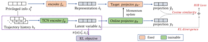
Figure 1: HIB adopts the IB principle to recover the privileged knowledge from a fixed length of local history information. The RL objective also provides gradients to the history encoder $f_{\psi}$, implying that the learned representation can be combined with any RL algorithm effectively.

5.2 Historical Information Bottleneck

We first briefly introduce the IB principle. In a supervised setting that aims to learn a representation $Z$ of a given input source $X$ with the target source $Y$, IB maximizes the MI between $Z$ and $Y$ (i.e., max $I(Z;Y)$) and restricts the complexity of $Z$ using the constraint as $I(Z;X)<I_{c}$. Combining the two terms, the IB objective is equal to $\max I(Z;Y)-\alpha I(Z;X)$ with a Lagrange multiplier $\alpha$.

To optimize the MI in Eq. (10) via contrastive objective [9], we introduce a historical representation $z_{t}\sim f_{\psi}(h_{t})$ to extract useful features that contain privileged information from a long historical vector $h_{t}$, where $f_{\psi}$ is a temporal convolution network (TCN) [4] that captures long-term information along the time dimension. We use another notation $\psi$ to distinguish it from the predictive encoder $\phi_{1}$ in Eq. (10), since the contrastive objective and predictive objective $I_{\rm pred}$ learn distinct representations by optimizing different variational bounds. In our IB objective, the input variable is $H_{t}$ and the corresponding target variable is $S^{p}_{t}$. Our objective is to maximize the MI term $I(Z_{t};\mathcal{S}^{p}_{t})$ while minimizing the MI term $I(H_{t};Z_{t})$ with $Z_{t}=f_{\psi}(H_{t})$, which takes the form of

$$\min-I(Z_{t};S^{p}_{t})+\alpha I(H_{t};Z_{t}),$$ (11)

where $\alpha$ is a Lagrange multiplier. The $I(Z_{t};S^{p}_{t})$ term quantifies the amount of information about the privileged knowledge preserved in $Z_{t}$, and the $I(H_{t};Z_{t})$ term is a regularizer that controls the complexity of representation learning. With a well-tuned $\alpha$, we do not discard useful information that is relevant to the privileged knowledge.

We minimize the MI term $I(H_{t};Z_{t})$ in Eq. (11) by minimizing a tractable upper bound. To this end, we introduce a variational approximation $q(z_{t})$ to the intractable marginal $p(z_{t})=\int p(h_{t})p(z_{t}|h_{t})dh_{t}$. Specifically, the following upper-bound of $I(H_{t};Z_{t})$ holds,

$$I(H_{t};Z_{t})=\mathbb{E}_{p(z_{t},h_{t})}\Big{[}\log\frac{p(z_{t}|h_{t})}{p(z_{t})}\Big{]} =\mathbb{E}_{p(z_{t},h_{t})}\Big{[}\log\frac{p(z_{t}|h_{t})}{q(z_{t})}\Big{]}-D_{\rm KL}[p(z_{t})\|q(z_{t})]$$ (12)

$$\leq D_{\rm KL}[p(z_{t}|h_{t})\|q(z_{t})],$$

where the inequality follows the non-negativity of the KL divergence, and $q(z_{t})$ is an approximation of the marginal distribution of $Z_{t}$. We follow Alemi et al. [2] and use a spherical Gaussian $q(z_{t})=\mathcal{N}(0,I)$ as an approximation.

One can maximize the MI term $I(Z_{t};S^{p}_{t})$ in Eq. (11) based on the contrastive objective [9]. Specifically, for a given $s^{p}_{t}$, the positive sample $z_{t}\sim f_{\psi}(h_{t})$ is the feature of corresponding history in timestep $t$, and the negative sample $z^{-}$ can be extracted from randomly sampled historical vectors. However, considering unresolved trade-offs involved in negative sampling [46, 17], we try to simplify the contrastive objective without negative samples. In HIB, we empirically find that the performance does not decrease without negative sampling. Such a simplification was also adopted by recent contrastive methods for RL [37, 32]. Without negative sampling, the contrastive loss becomes a cosine similarity with only positive pairs.

We adopt a two-stream architecture to learn $z_{t}$, including an online and a target network. Each network contains an encoder and a projector, as shown in Fig. 1. The online network is trained to use history to predict the corresponding privilege representation. Given a pair of a history sequence and privileged state $(h_{t},s^{p}_{t})$, we obtain $\tilde{e}_{t}=f_{\omega}(s^{p}_{t})$ with an encoder $f_{\omega}$ to get the representation of $s^{p}_{t}$. Then we use TCN as the history encoder $f_{\psi}$ to learn the latent representation $z_{t}\sim f_{\psi}(\cdot|h_{t})$. Here $f_{\omega}$ is used to project $s^{p}_{t}$ in the same dimensional space as $z_{t}$, so $f_{\omega}$ can be an identity operator or a simple MLP in the case of dimension requirement (see Appendix C.1 for details of implementation). As $\tilde{e}_{t}$ and $z_{t}$ have the same dimensions, the projectors share the same architecture. The online projector $g_{\theta}$ outputs $y_{t}=g_{\theta}(z_{t})$ and the target projector $g_{\theta^{-}}$ outputs $\tilde{y}_{t}=g_{\theta^{-}}(\tilde{e}_{t})$. We use the following cosine similarity loss between $y_{t}$ and $\tilde{y}_{t}$, and use stop gradient ($\mathrm{sg}[\cdot]$) for the target value $\tilde{y}$, as

$$\mathcal{L}_{\rm sim}=-\sum_{y_{t},\hat{y}_{t}}\left(\frac{y_{t}}{\left\|y_{t}\right\|_{2}}\right)^{\top}\left(\frac{\mathrm{sg}[\tilde{y}_{t}]}{\left\|\mathrm{sg}[\tilde{y}_{t}]\right\|_{2}}\right),$$ (13)

Algorithm 1 Historcal Information Bottleneck (HIB)

# Training Process (sim)
Initialize: Buffer $\mathcal{D}=\{[s^{l}_{t},s^{p}_{t}],a_{t},r_{t},[s^{l}_{t+1},s^{p}_{t+1}],h_{t}\}$
Initialize: Historical encoder $f_{\psi}$, privilege encoder $f_{\omega}$, projector $g_{\theta}$ and target projector $g_{\theta^{-}}$.

1:  while not coverge do

2:     Interact to the environment to collect $(s^{o}_{i},a_{i},r_{i},s^{o}_{i+1})$ with privileged state and save it to $\mathcal{D}$

3:     for $j$ from 0 to $N$ do

4:        Sample a batch of $(s^{o}_{i},a_{i},r_{i},s^{o}_{i+1})$ with history $h_{i}$

5:        Feed online $z_{i}\sim f_{\psi}(h_{i})$, $y_{i}\leftarrow g_{\theta}(z_{i})$, and target network $\tilde{e}_{i}\leftarrow f_{\omega}(s^{p}_{i})$, $\tilde{y_{i}}\leftarrow g_{\theta^{-}}(\tilde{e_{i}})$

6:        Compute cosine similarity $\mathcal{L}_{\rm sim}(y_{i},\tilde{y_{i}})$, KL regularization $\mathcal{L}_{\rm KL}$ and RL objective $\mathcal{L}_{\rm RL}$

7:        Update the HIB parameters via Eq. (14)

8:     end for

9:  end while

# Evaluation Process (real)

1:  Reset the environment and obtain the initial $s_{0}$ and $h_{0}$

2:  for $t$ from $t_{0}$ to $t_{\rm max}$ do

3:     Estimate the privileged state via $z_{t}\sim f_{\psi}(h_{t})$, and select action via $a\sim\hat{\pi}(a|s^{l}_{t},z_{t})$

4:     Interact with the environment, obtain the next state, set $s_{t}^{l}\leftarrow s_{t+1}^{l}$, and update $h_{t}$

5:  end for

To prevent collapsed solutions in the two-stream architecture, we follow previous architectures [14] by using a momentum update for the target network to avoid collapsed solutions. Specifically, the parameter of the target network $\theta^{-}$ takes an exponential moving average of the online parameters $\theta$ with a factor $\tau\in[0,1]$, as $\theta^{-}\leftarrow\tau\theta^{-}+(1-\tau)\theta$.

At each training step, we perform a stochastic optimization step to minimize $\mathcal{L}_{\rm sim}$ with respect to $\theta$ and $\psi$. Meanwhile, we learn an RL policy $\pi(a|s^{l}_{t},z_{t})$ based on the historical representation $z_{t}$, and the RL objective is also used to train the TCN encoder $f_{\psi}$. The dynamics are summarized as

$$\theta\leftarrow{\rm optimizer}(\theta,\nabla_{\theta}\mathcal{L}_{\rm sim}),\quad\psi\leftarrow{\rm optimizer}(\psi,\nabla_{\psi}\big{(}\lambda_{1}\mathcal{L}_{\rm sim}+\lambda_{2}\mathcal{L}_{\rm KL}+\mathcal{L}_{\rm RL}(s^{l}_{t},z_{t})\big{)},$$ (14)

where $\mathcal{L}_{\rm KL}=D_{\rm KL}(f_{\psi}(h_{t})\|\mathcal{N}(0,I))$ is the IB term in Eq. (12) that controls the latent complexity, and $\mathcal{L}_{\rm RL}$ is the loss function for an arbitrary RL algorithm. We summarize the process in Alg. 1.

6 Experiments

6.1 Benchmarks and Compared Methods

To quantify the generalizability of the proposed HIB, we conduct experiments in simulated environments that include multiple domains for a comprehensive evaluation, and also the legged robot locomotion task to evaluate the generalizability in sim-to-real transfer.

Privileged DMC Benchmark. We conduct experiments on DeepMind Control Suite (DMC) [42] with manually defined privileged information, which contains dynamic parameters such as friction and torque strength. The privileged knowledge is only visible in the training process. Following Benjamins et al. [5], we randomize the privilege parameters at the beginning of each episode, and the randomization range can be different for training and testing. Specifically, we choose three randomization ranges for varied difficulty levels, i.e., ordinary, o.o.d., and far o.o.d.. The ordinary setting means that the test environment has the same randomization range as in training, while o.o.d. and far o.o.d. indicate that the randomization ranges are larger with different degrees, causing test environments being out-of-distribution compared with training environment. The detailed setup can be found in Appendix B.1. We evaluate the algorithms in three different domains, namely pendulum, finger spin, and quadruped walk, which cover various difficulties ranging from ordinary to far o.o.d.. This Privileged DMC benchmark is referred to as DMC benchmark in the following for simplicity.

Table 1: Evaluated episodic return achieved by HIB and baselines on DMC tasks. We report the mean and standard deviation for 100K steps. o.o.d. and far o.o.d. settings mean the randomization ranges in testing are larger than the range in training, indicating that the test environments are out-of-distribution (o.o.d) compared to the training environment. We refer to Appendix B.1 for the details.

Domain	Testing Difficulty	Teacher	HIB (ours)	SAC-DR	Student	Dropper
Pendulum	ordinary	$-98.29\pm 80.41$	$-110.33\pm 89.67$	$-206.33\pm 259.66$	$-107.69\pm 90.87$	$-204.90\pm 223.74$
	o.o.d.	$-251.16\pm 384.52$	$-271.25\pm 355.96$	$-502.58\pm 543.67$	$-401.39\pm 504.42$	$-436.82\pm 473.84$
	far o.o.d.	$-660.98\pm 535.22$	$-671.83\pm 531.42$	$-800.62\pm 583.95$	$-729.69\pm 551.88$	$-674.43\pm 520.75$
Finger Spin	ordinary	$826.19\pm 152.61$	$714.06\pm 233.85$	$529.32\pm 414.99$	$657.00\pm 411.07$	$569.56\pm 308.62$
	o.o.d.	$793.18\pm 196.02$	$669.21\pm 254.22$	$460.79\pm 417.85$	$649.58\pm 405.97$	$551.61\pm 318.03$
	far o.o.d.	$663.73\pm 292.41$	$645.42\pm 248.03$	$453.00\pm 396.03$	$598.76\pm 409.50$	$518.05\pm 293.88$
Quadruped Walk	ordinary	$272.38\pm 60.87$	$946.72\pm 31.43$	$224.02\pm 27.57$	$223.93\pm 112.70$	$334.45\pm 380.94$
	o.o.d.	$217.45\pm 121.08$	$927.91\pm 53.05$	$203.21\pm 38.98$	$207.11\pm 127.37$	$287.68\pm 352.45$
	far o.o.d.	$192.93\pm 124.30$	$904.72\pm 85.76$	$164.79\pm 64.32$	$173.41\pm 136.94$	$286.00\pm 347.52$

Table 2: Evaluated episodic return achieved by HIB and baselines of legged robot evaluated in the Isaac-Gym simulator. Results are averaged over 1000 trajectories with different difficulties. Reward designs follow [33] and environmental details can be achieved in Appendix B.2.

Terrain	Teacher	HIB (ours)	PPO-DR	Student	Dropper
Smooth Slope	$21.30\pm 2.49$	$21.16\pm 2.69$	$17.30\pm 2.67$	$21.13\pm 2.76$	$18.68\pm 2.96$
Rough Slope	$20.29\pm 2.76$	$19.94\pm 3.39$	$16.27\pm 2.89$	$20.24\pm 3.36$	$17.35\pm 3.44$
Stair up	$20.13\pm 2.07$	$18.47\pm 3.58$	$16.43\pm 2.38$	$18.34\pm 3.82$	$16.79\pm 3.22$
Stair down	$20.72\pm 3.66$	$18.35\pm 6.33$	$17.36\pm 4.26$	$18.26\pm 6.43$	$16.47\pm 4.14$
Obstacle	$21.95\pm 2.40$	$21.58\pm 3.28$	$17.34\pm 2.72$	$21.36\pm 3.54$	$20.14\pm 2.45$

Sim-to-Real Learning in Legged Robot. This experiment is conducted on a quadrupedal robot. In this domain, privileged knowledge is defined as terrain information (e.g. heights of surroundings) of the environment and dynamic information such as friction, mass, and damping of the quadrupedal robot. In simulation, we develop the training code based on the open-source codebase [33] for on-policy PPO in legged robot, which leverages the Isaac Gym simulator [25] to support simulation of massive robots in parallel. The simulated environment also provides multi-terrain simulation, including slopes, stairs, and discrete obstacles with automatic curriculum that adapts the task difficulty according to the performance. Details can be found in Appendix B.2. For policy generalization in the real robot, we utilize Unitree A1 robot [43] to facilitate the real-world deployment.

Baselines. We compare HIB to the following baselines. (i) Teacher policy is learned by oracle states with privileged knowledge. (ii) Student policy follows RMA [21] that mimics the teacher policy through supervised learning, with the same architecture as the history encoder in HIB. We remark that student needs a two-stage training process to obtain the policy. (iii) Dropper is implemented according to Li et al. [23], which gradually drops the privileged information and finally converts to a normal agent that only takes local states as input. (iv) DR agent utilizes domain randomization for generalization and is directly trained with standard RL algorithms with local states as input.

6.2 Simulation Comparison

For DMC benchmark, we choose SAC [15] as the basic RL algorithm to perform a fair comparison. For Legged Robot task, we adopt PPO [36] as the basic RL algorithm since previous studies show that PPO combined with massive parallelism obtains remarkable performance in challenging legged locomotion tasks [22, 21]. As described above, we uniformly sample privilege parameters episodically from a specified range for both training and testing. Thus, the agent needs to take actions in different underlying dynamics episodically, which is very different from the standard RL setting.

The results for DMC benchmark are shown in Table 1. Our method achieves the best performance in almost all test environments, especially in the most challenging task quadruped walk. Surprisingly, we find HIB even outperforms the teacher policy in this task. We hypothesize that this environment is stochastic, and the history of local states and actions contains more useful information that can benefit future decisions. In quadruped walk, an agent relies on the angles and positions of previous legged joints to make a smooth movement, which is somewhat more important than the current privileged state. HIB performing better in history utilization while other methods fail.

The results on Legged Robot benchmark (Table 2) further verify the advantage of HIB, where our method outperforms other baselines on most terrains except on rough slope. From the simulation results, HIB can be seamlessly combined with different RL algorithms and generalizes well across different domains and tasks, demonstrating the efficiency and high scalability of HIB.

6.3 Visualization and Ablation Study

To investigate the ability of HIB in modeling the privileged knowledge, we visualize the latent representation learned by HIB and the strongest baseline student via dimensional reduction with T-SNE [45]. We also visualize the true privileged information for comparison. The visualization is conducted in finger spin task and the results are given in Fig. 4. We find that the student agent can only recover part of the privileged knowledge that covers the bottom left and upper right of the true privilege distribution. In contrast, the learned representation of HIB has almost the same distribution as privileged information. This may help explain why our method outperforms other baselines and generalizes to o.o.d. scenarios without significant performance degradation.

We conduct an ablation study for each component of HIB to verify their effectiveness.

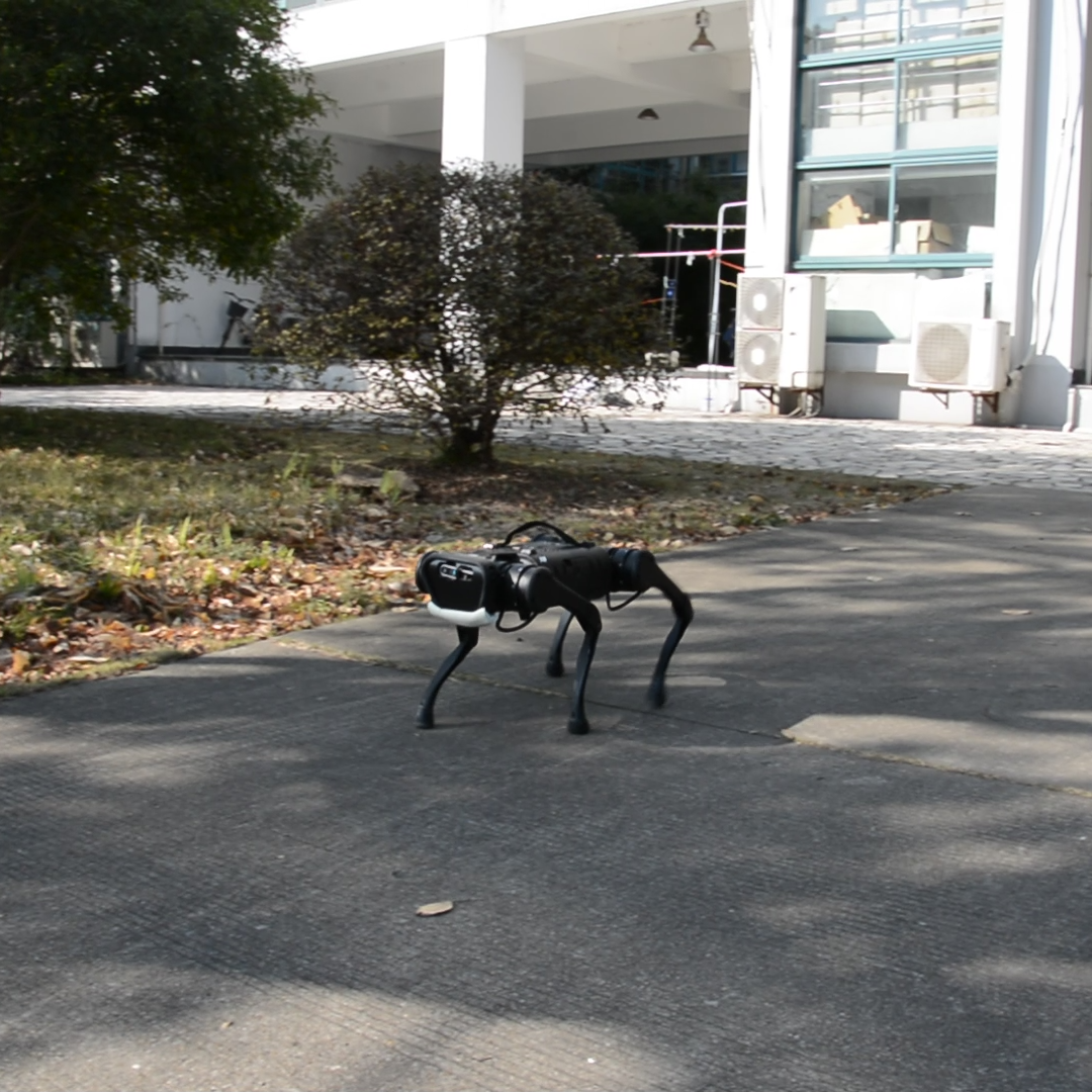
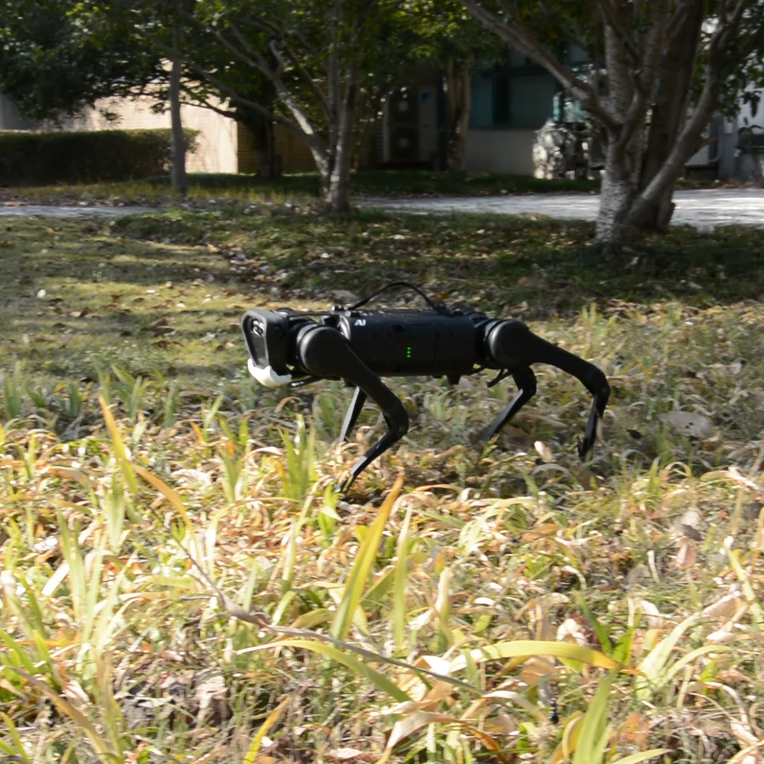
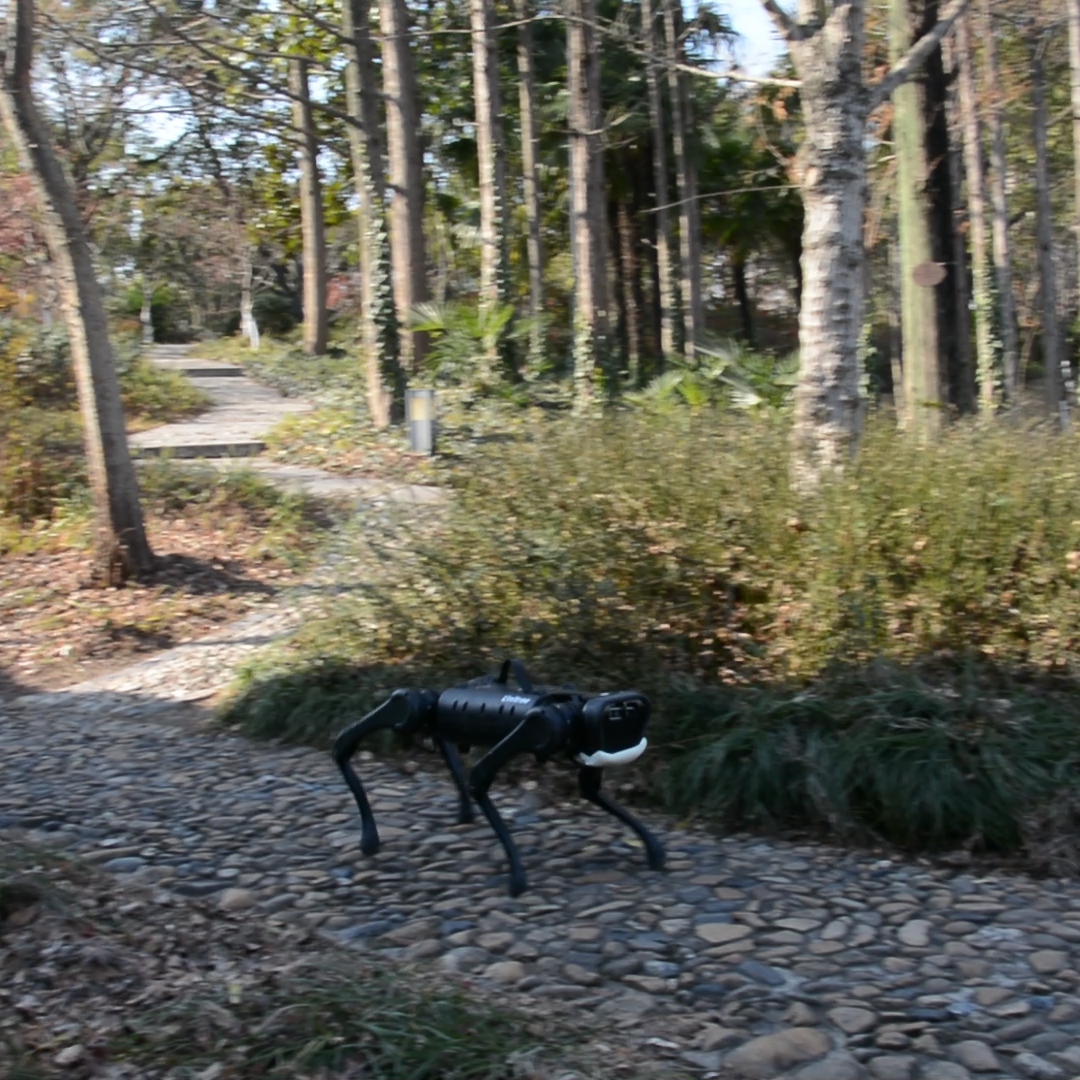
Figure 2: HIB is deployed on real A1 robot in flat, grass, and pebble without any fine-tuning. Videos available at https://bit.ly/3waXiNu.

Specifically, we design the following variants to compare with. (i) HIB-w/o-ib. This method only uses RL loss to update history encoder $f_{\psi}$, which is similar to a standard recurrent neural network policy. (ii) HIB-w/o-rl. This variant only uses HIB loss to update the history encoder without the RL objective. (iii) HIB-w/o-proj. We drop the projectors in HIB and directly compute cosine similarity loss between $z_{t}$ and $\tilde{e}_{t}$. (iv) HIB-contra. HIB-contra uses contrastive loss [39] instead of cosine similarity with a score function that assigns high scores for positive pairs and low scores for negative pairs.

From the result in Fig. 4, we observe that HIB-w/o-ib almost fails and HIB-w/o-rl can get relatively high scores, which signifies that both HIB loss and RL loss are important for the agent to learn a well-generalized policy, especially the HIB loss. The HIB loss helps agent learns a historical representation that contains privileged knowledge for better generalization. Furthermore, projectors and the momentum update mechanism are also crucial in learning robust and effective representation. Moreover, HIB-contra performs well at the beginning but fails later, which indicates that the contrastive objective requests constructing valid negative pairs and learning a good score function, which is challenging in the general state-based RL setting.

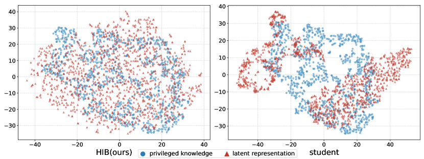
Figure 3: T-SNE visualization for the privilege representation and the learned latent representation of history encoder in finger spin.

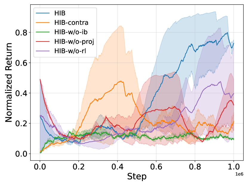
Figure 4: Comparison of different HIB variants in quadruped walk.

6.4 Real-world Application

To further evaluate the generalization performance of HIB in the real-world, we deploy the HIB policy trained in Legged Robot benchmark on a real-world A1 robot without any fine-tuning. Note that the policy is directly run on the A1 hardware and the local state is read or estimated from the onboard sensors and IMU, making the real-world control noisy and challenging. Fig. 2 shows the snapshots of HIB agent traversing flat, grass, and pebble terrains. The agent can generalize to different challenging terrains with stable control behavior and there is no failure in the whole experimental process. These real experiments demonstrate that HIB can help bridge the sim-to-real gap without any additional tuning in real environments.

7 Conclusion and Future Work

We propose a novel privileged knowledge distillation method based on the Information Bottleneck to narrow the knowledge gap between local and oracle RL environments. In particular, the proposed two-stream model design and HIB loss help reduce the performance discrepancy given in our theoretical analysis. Our experimental results on both simulated and real-world environments show that (i) HIB learns robust representations to reconstruct privileged knowledge from local historical trajectories and boosts the RL agent’s performance, and (ii) HIB can achieve improved generalizability in out-of-distribution environments compared to previous methods. In the future, we plan to extend our method to recover multi-modal privileged knowledge, which is more high-dimensional and complex.

Appendix A Theorems and Proofs

A.1 POMDP and Sim-to-Real Problems

We summarize common points and differences between POMDP and our setting as follows.

1. The transition function and reward function for both problems follows the ground-truth dynamics of the environment.

2. In POMDP, the agent cannot access the oracle state in both training and evaluation, while in sim-to-real adaptation, the agent can access the oracle in training (in the simulation).

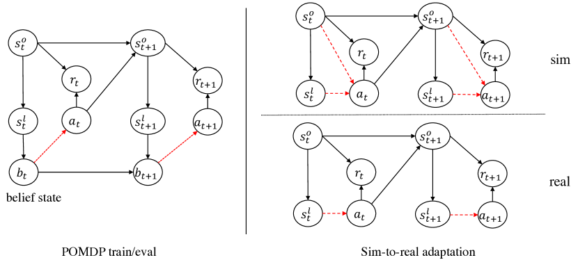
Figure 5: The difference between POMDP setting and the sim-to-real problem.

A.2 Proof of Theorem 1

We begin by deriving the imitation discrepancy bound in an ordinary MDP, as shown in the following theorem.

Theorem A.1 (General oracle imitation discrepancy bound).

Let the policy divergence between the oracle policy $\pi^{*}$ and the learned policy $\hat{\pi}$ is $\epsilon_{\pi}=\sup_{s}D_{\rm TV}(\pi^{*}(\cdot|s)\|\hat{\pi}(\cdot|s)).$ Then the difference between the optimal action value function $Q^{*}$ of $\pi^{*}$ and the action value function $\hat{Q}$ of $\hat{\pi}$ is bounded as

$$\sup_{s,a}\big{|}Q^{*}(s,a)-\hat{Q}(s,a)\big{|}\leq\frac{2\gamma r_{\rm max}}{(1-\gamma)^{2}}\epsilon_{\pi},$$ (15)

where $\gamma$ is the discount factor, and $r_{\rm max}$ is the maximum reward in each step.

Proof.

For any $(s,a)$ pair that $s\in\mathcal{S},a\in\mathcal{A}$, the difference between $Q^{*}(s,a)$ and $\hat{Q}(s,a)$ is

$$\>\>\>\>\>Q^{*}(s,a)-\hat{Q}(s,a)$$ (16)

$$=r(s,a)+\gamma\mathbb{E}_{s^{\prime}\sim P(s,a),a^{\prime}\sim\pi^{*}(\cdot|s^{\prime})}\big{[}Q^{*}(s^{\prime},a^{\prime})\big{]}-r(s,a)-\gamma\mathbb{E}_{s^{\prime}\sim P(s,a),a^{\prime\prime}\sim\hat{\pi}(\cdot|s^{\prime})}\big{[}\hat{Q}(s^{\prime},a^{\prime\prime})\big{]}$$

$$=\gamma\sum_{s^{\prime},a^{\prime}}P(s^{\prime}|s,a)\big{[}\pi^{*}(a^{\prime}|s^{\prime})Q^{*}(s^{\prime},a^{\prime})-\hat{\pi}(a^{\prime}|s^{\prime})\hat{Q}(s^{\prime},a^{\prime})\big{]}.$$

Then we introduce some intermediate terms and obtain

$$\>\>\>\>\>Q^{*}(s,a)-\hat{Q}(s,a)$$ (17)

$$=\gamma\sum_{s^{\prime},a^{\prime}}P(s^{\prime}|s,a)\big{[}\pi^{*}(a^{\prime}|s^{\prime})Q^{*}(s^{\prime},a^{\prime})-\pi^{*}(a^{\prime}|s^{\prime})\hat{Q}(s^{\prime},a^{\prime})+\pi^{*}(a^{\prime}|s^{\prime})\hat{Q}(s^{\prime},a^{\prime})-\hat{\pi}(a^{\prime}|s^{\prime})\hat{Q}(s^{\prime},a^{\prime})\big{]}$$

$$=\gamma\sum_{s^{\prime},a^{\prime}}P(s^{\prime}|s,a)\pi^{*}(a^{\prime}|s^{\prime})\big{[}Q^{*}(s^{\prime},a^{\prime})-\hat{Q}(s^{\prime},a^{\prime})\big{]}+\gamma\sum_{s^{\prime},a^{\prime}}P(s^{\prime}|s,a)\hat{Q}(s^{\prime},a^{\prime})\big{[}\pi^{*}(a|s)-\hat{\pi}(a|s)\big{]}$$

$$\leq\gamma\big{\|}Q^{*}-\hat{Q}\big{\|}_{\infty}+\gamma\big{\|}P\hat{Q}\big{\|}_{\infty}\big{\|}\pi^{*}-\hat{\pi}\big{\|}_{1}\qquad\qquad\qquad\qquad\qquad\rhd\text{H{\"{o}}lder's inequality}$$

$$\leq\gamma\big{\|}Q^{*}-\hat{Q}\big{\|}_{\infty}+2\gamma\big{\|}\hat{Q}\big{\|}_{\infty}\epsilon_{\pi}$$

$$\leq\gamma\big{\|}Q^{*}-\hat{Q}\big{\|}_{\infty}+\frac{2\gamma r_{\rm max}}{1-\gamma}\epsilon_{\pi}.\qquad\qquad\qquad\qquad\qquad\qquad\rhd~{}\hat{Q}(s,a)\leq\frac{r_{\rm max}}{1-\gamma},\forall s,a$$

Thus,

$$\big{\|}Q^{*}-\hat{Q}\big{\|}_{\infty}-\gamma\big{\|}Q^{*}-\hat{Q}\big{\|}_{\infty} \leq\frac{2\gamma r_{\rm max}}{1-\gamma}\epsilon_{\pi}$$ (18)

$$(1-\gamma)\big{\|}Q^{*}-\hat{Q}\big{\|}_{\infty} \leq\frac{2\gamma r_{\rm max}}{1-\gamma}\epsilon_{\pi}.$$

Then we have

$$\big{\|}Q^{*}-\hat{Q}\big{\|}_{\infty}\leq\frac{2\gamma r_{\rm max}}{(1-\gamma)^{2}}\epsilon_{\pi},$$ (19)

which completes our proof. ∎

Next, we consider the value discrepancy bound in policy imitation with the knowledge gap. Specifically, we denote the optimal value function with oracle states $s^{o}=[s^{l},s^{p}]$ as $Q^{*}(s^{l},s^{p},a)$, and the value function with local states as $Q(s^{l},a)$. Then we have the following discrepancy bound (restate of Theorems 1).

Theorem A.2 (Policy imitation discrepancy).

The value discrepancy between the optimal value function with privileged knowledge and the value function with local state is bounded as

$$\sup_{s^{l},s^{p},a}\big{|}Q^{*}(s^{l},s^{p},a)-\hat{Q}^{\hat{\pi}}(s^{l},a)\big{|}\leq\frac{2\gamma r_{\rm max}}{(1-\gamma)^{2}}\epsilon_{\hat{\pi}},$$ (20)

where

$$\epsilon_{\hat{\pi}}=\sup_{s^{l},s^{p}}D_{\rm TV}(\pi^{*}(\cdot|s^{l},s^{p})\|\hat{\pi}(\cdot|s^{l}))$$ (21)

is the policy divergence between $\pi^{*}$ and $\hat{\pi}$, and $r_{\rm max}$ is the maximum reward in each step.

Proof.

We note that the transition functions for learning $\hat{\pi}(a|s^{l})$ and $\pi^{*}(a|s^{l},s^{p})$ are the same and follow the ground-truth dynamics. Although we cannot observe the privileged state $s^{p}$ in learning the local policy, the transition of the next state $P(s^{l}_{t+1},s^{o}_{t+1}|s^{l}_{t},s^{p}_{t})$ still depends on the oracle state of the previous step that contains the privileged state $s^{p}_{t}$. Since the agent is directly interacting with the environment, the privileged state does affect the transition functions. As a result, for policy imitation of the local policy, we have a similar derivation as in (16) because the transition function in (16) is the same for $\pi^{*}(a_{t+1}|s^{o}_{t+1})Q^{*}(s^{o}_{t+1},a_{t+1})$ and $\hat{\pi}(a_{t+1}|s^{l}_{t+1})\hat{Q}(s^{l}_{t+1},a_{t+1})$, which leads to a similar discrepancy bound as in an ordinary MDP. ∎

A.3 Proof of Theorem 2

We have defined the history encoder $\hat{P}_{\phi}$ which takes the history as input and the privileged state as output:

$$\hat{s}^{p}_{t}=\hat{P}(\cdot|h_{t}).$$ (22)

In the following, we give the performance discrepancy bound between the optimal value function with oracle state $s^{o}_{t}=[s^{l}_{t},s^{p}_{t}]$ and the value function with local state $s^{l}_{t}$ as well as the predicted privileged state $\hat{s}^{p}_{t}$ (restate of Theorem 2).

Theorem A.3 (Privilege modeling discrepancy).

Let the divergence between the privileged state model $\hat{P}(s^{p}_{t+1}|h_{t+1})$ and the true distribution of privileged state $P(s^{p}_{t+1}|h_{t+1})$ be bounded as

$$\epsilon_{\hat{P}}=\sup_{t\geq t_{0}}\sup_{h_{t+1}}D_{\rm TV}\big{(}P(\cdot\>|\>h_{t+1})\>\|\>\hat{P}(\cdot\>|\>h_{t+1})\big{)}.$$ (23)

Then the performance discrepancy bound between the optimal value function with $P$ and the value function with $\hat{P}$ holds, as

$$\sup_{t\geq t_{0}}\sup_{s^{l},s^{p},a}|Q^{*}(s^{l}_{t},s^{p}_{t},a_{t})-\hat{Q}_{t}(s^{l}_{t},\hat{s}^{p}_{t},a_{t})|\leq\frac{\Delta_{\mathbb{E}}}{(1-\gamma)}+\frac{2\gamma r_{\rm max}}{(1-\gamma)^{2}}\epsilon_{\hat{P}},$$ (24)

where $\Delta_{\mathbb{E}}=\sup_{t\geq t_{0}}\big{\|}Q^{*}-\mathbb{E}_{s^{p}_{t}\sim P(\cdot|h_{t})}[Q^{*}]\big{\|}_{\infty}+\big{\|}\hat{Q}-\mathbb{E}_{\hat{s}^{p}_{t}\sim\hat{P}(\cdot|h_{t})}[\hat{Q}]\big{\|}_{\infty}$ is the difference in the same value function with sampled $s^{p}_{t}$ and the expectation of $s^{p}_{t}$ conditioned on $h_{t}$.

Proof.

For $\hat{Q}$ that estimates the value function of state $(s^{l}_{t},\hat{s}^{p}_{t})$, the value is stochastic since the hidden prediction $\hat{s}^{p}_{t}$ is a single sample from the output of model $\hat{P}(\cdot|h_{t})$. We take the expectation to the output of $\hat{P}(\cdot|h_{t})$ and obtain the expected $\hat{Q}$ as

$$\>\>\>\mathbb{E}_{\hat{s}^{p}_{t}\sim\hat{P}(\cdot|h_{t})}[\hat{Q}_{t}(s^{l}_{t},\hat{s}^{p}_{t},a_{t})]$$ (25)

$$=\mathbb{E}_{s^{p}_{t}\sim P(\cdot|h_{t})}[r(s^{l}_{t},s^{p}_{t})]+\gamma\mathbb{E}_{s^{l}_{t+1}\sim P(\cdot|h_{t},a_{t}),\hat{s}^{p}_{t+1}\sim\hat{P}(\cdot|h_{t},a_{t},s^{l}_{t+1})}\big{[}\max_{a^{\prime}}\hat{Q}_{t+1}(s^{l}_{t+1},\hat{s}^{p}_{t+1},a^{\prime})\big{]}\quad\rhd{\eqref{eq:app-thm2-model}}$$

$$=\mathbb{E}_{s^{p}_{t}\sim P(\cdot|h_{t})}[r(s^{l}_{t},s^{p}_{t})]+\gamma\mathbb{E}_{s^{l}_{t+1}\sim P(\cdot|h_{t},a_{t}),\hat{s}^{p}_{t+1}\sim\hat{P}(\cdot|h_{t+1})}\big{[}\max_{a^{\prime}}\hat{Q}_{t+1}(s^{l}_{t+1},\hat{s}^{p}_{t+1},a^{\prime})\big{]},$$

where $h_{t+1}=h_{t}\cup\{s^{l}_{t+1},a_{t}\}$. We remark that the reward function $r(s^{l}_{t},s^{p}_{t})$ is returned by the real environment, thus $s^{p}_{t}$ follows the true $P$ in the reward.

Remark 1 (Explanation of the Bellman Equation).

Our goal is to fit the Bellman equation in (25). Fitting the Bellman equation in (25) has several benefits. Firstly, it is easily implemented based on the fitted privileged state model $\hat{P}$. Specifically, solving (25) is almost the same as solving an ordinary MDP, with $\hat{s}^{p}_{t}$ generated by $\hat{P}$ based on the history in place of the true privileged state of $s^{p}_{t}$ (which is unavailable). Secondly and most importantly, when the history is sufficiently strong in predicting $s^{p}_{t}$, solving (25) leads to approximately optimal solutions, as we show in this theorem.

For $Q^{*}$ that represents the optimal value function with the true privileged state, we have

$$Q^{*}(s^{l}_{t},s^{p}_{t},a_{t}) =r(s^{l}_{t},s^{p}_{t})+\gamma\mathbb{E}_{(s^{l}_{t+1},s^{p}_{t+1})\sim P(\cdot|s^{l}_{t},s^{p}_{t},a_{t})}[\max_{a^{\prime}}Q^{*}_{t+1}(s^{l}_{t+1},s^{p}_{t+1},a^{\prime})]$$ (26)

$$=r(s^{l}_{t},s^{p}_{t})+\gamma\mathbb{E}_{(s^{l}_{t+1},s^{p}_{t+1})\sim P(\cdot|h_{t},s^{p}_{t},a_{t})}[\max_{a^{\prime}}Q^{*}_{t+1}(s^{l}_{t+1},s^{p}_{t+1},a^{\prime})],$$

where the second equation holds since $h_{t}$ contains $s^{l}_{t}$. Then we take a similar expectation to the true hidden transition function $P$ as

$$\>\>\>\mathbb{E}_{s^{p}_{t}\sim P(\cdot|h_{t})}[Q^{*}(s^{l}_{t},s^{p}_{t},a_{t})]$$ (27)

$$=\mathbb{E}[r(s^{l}_{t},s^{p}_{t})]+\gamma\mathbb{E}_{(s^{l}_{t+1},s^{p}_{t+1})\sim P(\cdot|h_{t},s^{p}_{t},a_{t}),s^{p}_{t}\sim P(\cdot|h_{t})}[\max_{a^{\prime}}Q^{*}_{t+1}(s^{l}_{t+1},s^{p}_{t+1},a^{\prime})]$$

$$=\mathbb{E}[r(s^{l}_{t},s^{p}_{t})]+\gamma\mathbb{E}_{(s^{l}_{t+1},s^{p}_{t+1})\sim P(\cdot|h_{t},a_{t})}[\max_{a^{\prime}}Q^{*}_{t+1}(s^{l}_{t+1},s^{p}_{t+1},a^{\prime})]\qquad\qquad\rhd\text{according to Fig.~{}\ref{fig:graph-RL}}$$

$$=\mathbb{E}[r(s^{l}_{t},s^{p}_{t})]+\gamma\mathbb{E}_{s^{l}_{t+1}\sim P(\cdot|h_{t},a_{t}),s^{p}_{t+1}\sim P(\cdot|h_{t},a_{t},s^{l}_{t+1})}[\max_{a^{\prime}}Q^{*}_{t+1}(s^{l}_{t+1},s^{p}_{t+1},a^{\prime})]$$

$$=\mathbb{E}[r(s^{l}_{t},s^{p}_{t})]+\gamma\mathbb{E}_{s^{l}_{t+1}\sim P(\cdot|h_{t},a_{t}),s^{p}_{t+1}\sim P(\cdot|h_{t+1})}[\max_{a^{\prime}}Q^{*}_{t+1}(s^{l}_{t+1},s^{p}_{t+1},a^{\prime})],$$

where the last equation follows $h_{t+1}=h_{t}\cup\{s^{l}_{t+1},a_{t}\}$, and the second equation follows the causal graph shown in Fig. 6. Specifically, following the relationship in Fig. 6, we have

$$P(s^{o}_{t+1},h_{t},s^{p}_{t},a_{t})=P(h_{t})P(s^{p}_{t}|h_{t})P(a_{t}|h_{t})P(s^{o}_{t+1}|h_{t},s^{p}_{t},a_{t}).$$ (28)

Then we have

$$P(s^{o}_{t+1}|h_{t},s^{p}_{t},a_{t})P(s^{p}_{t}|h_{t}) =\frac{P(s^{o}_{t+1},h_{t},s^{p}_{t},a_{t})}{P(h_{t})P(s^{p}_{t}|h_{t})P(a_{t}|h_{t})}P(s^{p}_{t}|h_{t})=\frac{P(s^{o}_{t+1},h_{t},s^{p}_{t},a_{t})}{P(h_{t})P(a_{t}|h_{t})}$$ (29)

$$=\frac{P(s^{o}_{t+1},h_{t},s^{p}_{t},a_{t})}{P(a_{t},h_{t})}=P(s^{o}_{t+1},s^{p}_{t}|h_{t},a_{t}),$$

where we denote $s^{o}_{t+1}=[s_{t+1}^{l},s_{t+1}^{p}]$.

Figure 6: The causal graph. The agent takes action $a_{t}$ by only considering local states without accessing the privileged state $s^{p}_{t}$. The privileged state is based on history $h_{t}$. The next-state is conditional on $h_{t}$, $s^{p}_{t}$, and $a_{t}$.

Based on above analysis, we derive the value discrepancy bound as follows. For $\forall s^{l}_{t},s^{p}_{t},a_{t}$, the discrepancy between $Q^{*}(s^{l}_{t},s^{p}_{t},a_{t})$ and $\hat{Q}_{t}(s^{l}_{t},\hat{s}^{p}_{t},a_{t})$ can be decomposed as

$$\>\>\>\>\>Q^{*}(s^{l}_{t},s^{p}_{t},a_{t})-\hat{Q}_{t}(s^{l}_{t},\hat{s}^{p}_{t},a_{t})$$ (30)

$$=\underbrace{Q^{*}(s^{l}_{t},s^{p}_{t},a_{t})-\mathbb{E}_{s^{p}_{t}\sim P(\cdot|h_{t})}[Q^{*}(s^{l}_{t},s^{p}_{t},a_{t})]}_{(i)\Delta^{*}_{\mathbb{E}}}\underbrace{-\hat{Q}_{t}(s^{l}_{t},\hat{s}^{p}_{t},a_{t})+\mathbb{E}_{\hat{s}^{p}_{t}\sim\hat{P}(\cdot|h_{t})}[\hat{Q}_{t}(s^{l}_{t},\hat{s}^{p}_{t},a_{t})]}_{(ii)-\hat{\Delta}_{\mathbb{E}}}$$

$$\qquad\underbrace{+\mathbb{E}_{s^{p}_{t}\sim P(\cdot|h_{t})}[Q^{*}(s^{l}_{t},s^{p}_{t},a_{t})]-\mathbb{E}_{s^{p}_{t}\sim P(\cdot|h_{t})}[\hat{Q}_{t}(s^{l}_{t},s^{p}_{t},a_{t})]}_{(iii)\text{~{}value error}}$$

$$\qquad\underbrace{+\mathbb{E}_{s^{p}_{t}\sim P(\cdot|h_{t})}[\hat{Q}_{t}(s^{l}_{t},s^{p}_{t},a_{t})]-\mathbb{E}_{\hat{s}^{p}_{t}\sim\hat{P}(\cdot|h_{t})}[\hat{Q}_{t}(s^{l}_{t},\hat{s}^{p}_{t},a_{t})]}_{(iv)\text{~{}model error}},$$

where we add three terms with positive sign and negative sign, including $Q^{*}$ with the expectation of $P(\cdot|h_{t})$, $\hat{Q}_{t}$ with the expectation of $P(\cdot|h_{t})$, and $\hat{Q}_{t}$ with the expectation of $\hat{P}(\cdot|h_{t})$.

For $(i)$ and $(ii)$, we take the absolute value and get $\Delta_{\mathbb{E}}^{*}-\hat{\Delta}_{\mathbb{E}}\leq|\Delta_{\mathbb{E}}^{*}|+|\hat{\Delta}_{\mathbb{E}}|=\Delta_{\mathbb{E}}$, where

$$\Delta_{\mathbb{E}}^{*}-\hat{\Delta}_{\mathbb{E}}\leq|\Delta_{\mathbb{E}}^{*}|+|\hat{\Delta}_{\mathbb{E}}|\leq\sup_{s^{l}_{t},s^{p}_{t},a}\big{(}|\Delta_{\mathbb{E}}^{*}|+|\hat{\Delta}_{\mathbb{E}}|\big{)}$$ (31)

$$=\sup_{s^{l}_{t},s^{p}_{t},a}\big{|}Q^{*}(s^{l}_{t},s^{p}_{t},a)-\mathbb{E}_{s^{p}_{t}\sim P(\cdot|h_{t})}[Q^{*}(s^{l}_{t},s^{p}_{t},a)]\big{|}+\big{|}\hat{Q}_{t}(s^{l}_{t},s^{p}_{t},a)-\mathbb{E}_{\hat{s}^{p}_{t}\sim\hat{P}(\cdot|h_{t})}[\hat{Q}_{t}(s^{l}_{t},\hat{s}^{p}_{t},a)]\big{|}$$

$$=\big{\|}Q^{*}-\mathbb{E}_{s^{p}_{t}\sim P(\cdot|h_{t})}[Q^{*}]\big{\|}_{\infty}+\big{\|}\hat{Q}-\mathbb{E}_{\hat{s}^{p}_{t}\sim\hat{P}(\cdot|h_{t})}[\hat{Q}]\big{\|}_{\infty},$$

which represents the difference in the same value function caused by the expectation of $s^{p}_{t}$ with respect to the history.

For $(iii)$ that represents the value difference in the optimal value function $Q^{*}$ and the current value function $\hat{Q}$ with the same distribution of state-action, we have the following bound as

$$\>\>\>\>\mathbb{E}_{s^{p}_{t}\sim P(\cdot|h_{t})}[Q^{*}(s^{l}_{t},s^{p}_{t},a_{t})]-\mathbb{E}_{s^{p}_{t}\sim P(\cdot|h_{t})}[\hat{Q}_{t}(s^{l}_{t},s^{p}_{t},a_{t})]$$ (32)

$$=\mathbb{E}[r(s^{l}_{t},s^{p}_{t})]+\gamma\mathbb{E}_{s^{l}_{t+1}\sim P(\cdot|h_{t},a_{t}),s^{p}_{t+1}\sim P(\cdot|h_{t+1})}[\max_{a^{\prime}}Q^{*}(s^{l}_{t+1},s^{p}_{t+1},a^{\prime})]$$

$$\qquad-\mathbb{E}[r(s^{l}_{t},s^{p}_{t})]+\gamma\mathbb{E}_{s^{l}_{t+1}\sim P(\cdot|h_{t},a_{t}),s^{p}_{t+1}\sim P(\cdot|h_{t+1})}[\max_{a^{\prime\prime}}\hat{Q}_{t+1}(s^{l}_{t+1},s^{p}_{t+1},a^{\prime\prime})]\qquad\rhd\text{from~{}}\eqref{eq:thm-hidden-2}$$

$$=\gamma\mathbb{E}_{s^{l}_{t+1}\sim P(\cdot|h_{t},a_{t}),s^{p}_{t+1}\sim P(\cdot|h_{t+1})}[\max_{a^{\prime}}Q^{*}(s^{l}_{t+1},s^{p}_{t+1},a^{\prime})-\max_{a^{\prime\prime}}\hat{Q}_{t+1}(s^{l}_{t+1},s^{p}_{t+1},a^{\prime\prime})]$$

$$\leq\gamma\max_{a^{\prime}}\mathbb{E}_{s^{l}_{t+1}\sim P(\cdot|h_{t},a_{t}),s^{p}_{t+1}\sim P(\cdot|h_{t+1})}[Q^{*}(s^{l}_{t+1},s^{p}_{t+1},a^{\prime})-\hat{Q}_{t+1}(s^{l}_{t+1},s^{p}_{t+1},a^{\prime})]$$

$$\leq\gamma\sup_{s^{l}_{t+1},s^{p}_{t+1},a^{\prime}}\big{|}Q^{*}(s^{l}_{t+1},s^{p}_{t+1},a^{\prime})-\hat{Q}_{t+1}(s^{l}_{t+1},s^{p}_{t+1},a^{\prime})\big{|}$$

$$=\gamma\big{\|}Q^{*}-\hat{Q}_{t+1}\big{\|}_{\infty}.$$

For $(iv)$ that represents the model difference of hidden state with different distributions, we have the following bound by following (25), as

$$\>\>\>\>\mathbb{E}_{s^{p}_{t}\sim P(\cdot|h_{t})}[\hat{Q}_{t}(s^{l}_{t},s^{p}_{t},a_{t})]-\mathbb{E}_{\hat{s}^{p}_{t}\sim\hat{P}(\cdot|h_{t})}[\hat{Q}_{t}(s^{l}_{t},\hat{s}^{p}_{t},a_{t})]$$ (33)

$$=\mathbb{E}[r(s^{l}_{t},s^{p}_{t})]+\gamma\mathbb{E}_{s^{l}_{t+1}\sim P(\cdot|h_{t},a_{t}),s^{p}_{t+1}\sim P(\cdot|h_{t+1})}[\max_{a^{\prime}}\hat{Q}_{t+1}(s^{l}_{t+1},s^{p}_{t+1},a^{\prime})]$$

$$\qquad\qquad-\mathbb{E}[r(s^{l}_{t},s^{p}_{t})]-\gamma\mathbb{E}_{s^{l}_{t+1}\sim P(\cdot|h_{t},a_{t}),\hat{s}^{p}_{t+1}\sim\hat{P}(\cdot|h_{t+1})}[\max_{a^{\prime\prime}}\hat{Q}_{t+1}(s^{l}_{t+1},\hat{s}^{p}_{t+1},a^{\prime\prime})]$$

$$=\gamma\mathbb{E}_{s^{l}_{t+1}\sim P(\cdot|h_{t},a_{t})}\big{[}\mathbb{E}_{s^{p}_{t+1}\sim P(\cdot|h_{t+1})}[\max_{a^{\prime}}\hat{Q}_{t+1}(s^{l}_{t+1},s^{p}_{t+1},a^{\prime})]-\mathbb{E}_{\hat{s}^{p}_{t+1}\sim\hat{P}(\cdot|h_{t+1})}[\max_{a^{\prime\prime}}\hat{Q}_{t+1}(s^{l}_{t+1},\hat{s}^{p}_{t+1},a^{\prime\prime})]\big{]}$$

$$=\gamma\mathbb{E}_{s^{l}_{t+1}\sim P(\cdot|h_{t},a_{t})}\sum_{s^{p}_{t+1}}\max_{a^{\prime}}\hat{Q}_{t+1}(s^{l}_{t+1},s^{p}_{t+1},a^{\prime})P(s^{p}_{t+1}|h_{t+1})-\max_{a^{\prime\prime}}\hat{Q}_{t+1}(s^{l}_{t+1},s^{p}_{t+1},a^{\prime\prime})\hat{P}(s^{p}_{t+1}|h_{t+1}).$$

Define a new function as $F_{t+1}(s^{l}_{t+1},s^{p}_{t+1})=\max_{a}\hat{Q}_{t+1}(s^{l}_{t+1},s^{p}_{t+1},a)$, then we have

$$\>\>\>\>\mathbb{E}_{s^{p}_{t}\sim P(\cdot|h_{t})}[\hat{Q}_{t}(s^{l}_{t},s^{p}_{t},a_{t})]-\mathbb{E}_{\hat{s}^{p}_{t}\sim\hat{P}(\cdot|h_{t})}[\hat{Q}_{t}(s^{l}_{t},\hat{s}^{p}_{t},a_{t})]$$ (34)

$$=\gamma\mathbb{E}_{s^{l}_{t+1}\sim P(\cdot|h_{t},a_{t})}\sum_{s^{p}_{t+1}}F_{t+1}(s^{l}_{t+1},s^{p}_{t+1})P(s^{p}_{t+1}|h_{t+1})-F_{t+1}(s^{l}_{t+1},s^{p}_{t+1})\hat{P}(s^{p}_{t+1}|h_{t+1})$$

$$\leq\gamma\mathbb{E}_{s^{l}_{t+1}\sim P(\cdot|h_{t},a_{t})}\sum_{s^{p}_{t+1}}F_{t+1}(s^{l}_{t+1},s^{p}_{t+1})\big{|}P(s^{p}_{t+1}|h_{t+1})-\hat{P}(s^{p}_{t+1}|h_{t+1})\big{|}$$

$$\leq\gamma F_{\rm max}\big{\|}P(\cdot|h_{t+1})-\hat{P}(\cdot|h_{t+1})\big{\|}_{1}\qquad\qquad\qquad\qquad\qquad\qquad\rhd\text{H{\"{o}}lder's inequality}$$

$$=\frac{2\gamma r_{\rm max}}{1-\gamma}D_{\rm TV}(P(\cdot|h_{t+1})\|\hat{P}(\cdot|h_{t+1}))\qquad\qquad\qquad\qquad\qquad\qquad\rhd{F_{\rm max}\leq\nicefrac{{r_{\rm max}}}{{1-\gamma}}}$$

According to derivation of $(i)\sim(iv)$, we take the supreme of $s^{l}_{t},s^{p}_{t},a_{t}$ and obtain the discrepancy between $Q^{*}(s^{l}_{t},s^{p}_{t},a_{t})$ and $\hat{Q}_{t}(s^{l}_{t},\hat{s}^{p}_{t},a_{t})$ as

$$\|Q^{*}-\hat{Q}_{t}\|_{\infty} \leq\sup_{s^{l}_{t},s^{p}_{t},a}\big{(}|\Delta_{\mathbb{E}}^{*}|+|\hat{\Delta}_{\mathbb{E}}|\big{)}+\frac{2\gamma r_{\rm max}}{1-\gamma}D_{\rm TV}(P(\cdot|h_{t+1})\|\hat{P}(\cdot|h_{t+1}))+\gamma\|Q^{*}-\hat{Q}_{t+1}\|_{\infty}$$ (35)

$$\leq\sup_{s^{l}_{t},s^{p}_{t},a}\big{(}|\Delta_{\mathbb{E}}^{*}|+|\hat{\Delta}_{\mathbb{E}}|\big{)}+\frac{2\gamma r_{\rm max}}{1-\gamma}\epsilon_{\hat{P}_{t+1}}+\gamma\|Q^{*}-\hat{Q}_{t+1}\|_{\infty}$$

$$=\Delta_{\mathbb{E}}(t)+\frac{2\gamma r_{\rm max}}{1-\gamma}\epsilon_{\hat{P}_{t+1}}+\gamma\|Q^{*}-\hat{Q}_{t+1}\|_{\infty},$$

where we define

$$\epsilon_{\hat{P}_{t+1}}=\sup_{h_{t+1}}D_{\rm TV}(P(\cdot|h_{t+1})\|\hat{P}(\cdot|h_{t+1}))$$

as the model difference at time step $t+1$ with the worst-case history. Meanwhile, we define

$$\Delta_{\mathbb{E}}(t)=\sup_{s^{l}_{t},s^{p}_{t},a}\big{(}|\Delta_{\mathbb{E}}^{*}|+|\hat{\Delta}_{\mathbb{E}}|\big{)}\>\>=\>\>\underbrace{\big{\|}Q^{*}-\mathbb{E}_{s^{p}_{t}\sim P(\cdot|h_{t})}[Q^{*}]\big{\|}_{\infty}}_{\textrm{(i)}}\>+\>\underbrace{\big{\|}\hat{Q}-\mathbb{E}_{\hat{s}^{p}_{t}\sim\hat{P}(\cdot|h_{t})}[\hat{Q}]\big{\|}_{\infty}}_{\textrm{(ii)}},$$ (36)

to measure the difference in the same value function with true $s^{p}_{t}$ and the expectation of $s^{p}_{t}$ conditioned on history $h_{t}$.

In the following, we consider the step in worst case by taking supremum of $t$ when $t$ greater some $t_{0}$, and ensure the history is long and informative, as

$$\sup_{t\geq t_{0}}\|Q^{*}-\hat{Q}_{t}\|_{\infty} \leq\sup_{t\geq t_{0}}\Delta_{\mathbb{E}}(t)+\sup_{t\geq t_{0}}\frac{2\gamma r_{\rm max}}{1-\gamma}\epsilon_{\hat{P}_{t+1}}+\gamma\sup_{t\geq t_{0}}\|Q^{*}-\hat{Q}_{t+1}\|_{\infty}$$ (37)

$$\leq\sup_{t\geq t_{0}}\Delta_{\mathbb{E}}(t)+\sup_{t\geq t_{0}}\frac{2\gamma r_{\rm max}}{1-\gamma}\epsilon_{\hat{P}_{t+1}}+\gamma\sup_{t\geq t_{0}}\|Q^{*}-\hat{Q}_{t}\|_{\infty}$$

where we use inequality

$$\sup_{t\geq t_{0}}\|Q^{*}-\hat{Q}_{t+1}\|_{\infty}=\sup_{t\geq t_{0}+1}\|Q^{*}-\hat{Q}_{t}\|_{\infty}\leq\sup_{t\geq t_{0}}\|Q^{*}-\hat{Q}_{t}\|_{\infty}.$$

Then we have

$$\sup_{t\geq t_{0}}\|Q^{*}-\hat{Q}_{t}\|_{\infty} \leq\frac{\sup_{t\geq t_{0}}\Delta_{\mathbb{E}}(t)}{(1-\gamma)}+\sup_{t\geq t_{0}}\frac{2\gamma r_{\rm max}}{(1-\gamma)^{2}}\epsilon_{\hat{P}_{t+1}}$$ (38)

$$=\frac{\Delta_{\mathbb{E}}}{1-\gamma}+\frac{2\gamma r_{\rm max}}{(1-\gamma)^{2}}\epsilon_{\hat{P}},$$

where we define $\Delta_{\mathbb{E}}=\sup_{t\geq t_{0}}\Delta_{\mathbb{E}}(t)$ to consider the step of worst case by taking supremum of $t\geq t_{0}$. Meanwhile, we define the model error in worst case as

$$\epsilon_{\hat{P}}=\sup_{t\geq t_{0}}\epsilon_{\hat{P}}(t+1),$$ (39)

which can be minimized by using a neural network to represent $\hat{P}$, and reducing the error through Monte Carlo sampling of transitions in training.

We remark that in $\Delta_{\mathbb{E}}$ of Eq. (36), the term (i) in (36) captures how informative the history $h_{t}$ is in inferring necessary information of the hidden state $s^{p}_{t}$. Intuitively, term (i) characterizes the error in estimating the optimal $Q$-value with the informative history $h_{t}$. Similarly, term (ii) characterizes the error in predicting the hidden state $s^{p}_{t}$ that follows the estimated model $\hat{P}$ based on the history. If the model $\hat{P}$ is deterministic and each $\hat{s}^{p}_{t}\in\mathcal{S}^{p}$ has a corresponding history $h_{t}$, then term (ii) vanishes. Empirically, we use an informative history to make $\Delta_{\mathbb{E}}$ sufficiently small.

∎

Appendix B Environment Setting

B.1 Details of Privileged DMC Benchmark

Based on existing benchmarks [5, 42], we develop three environments for privileged knowledge distillation, including pendulum, finger spin, and quadruped walk, that cover various training difficulties from easy to difficult. Each environment defines a series of privilege parameters, which are indeed real-world physical properties, such as gravity, friction, or mass of an object. Such privilege parameters define the behavior of the environments, and are only visible in training and hidden in testing. In order to train a generalizable policy, we follow the domain randomization method and define a randomization range for privilege parameters for training. The underlying transition dynamics will change since we sample these privilege parameters uniformly from a pre-defined randomization range every episode. For policy evaluation, we additionally define two testing randomization ranges (o.o.d and far o.o.d) that contain out-of-distribution parameters compared to the training range. The privilege parameters and the corresponding ranges of each environment are listed in Table 3, Table 4, and Table 5, respectively. The training curves of this benchmark can be found in Fig. 7.

Table 3: Privileged knowledge randomization range on pendulum. The testing range (ordinary) is the same as the training range. The privilege parameter $d_{t}$ refers to the observation interval length, $g$ to gravity, $l$ to the pole length, $m$ to the pole mass.

Privilege Parameter	Training Range(ordinary)	Testing Range (o.o.d.)	Testing Range (far o.o.d.)
$d_{t}$	[0.0, 0.05]	[0.0, 0.1]	[0.0, 0.2]
$g$	[-2.0, 2.0]	[-3.0, 3.0]	[-4.0, 4.0]
$m$	[-0.5, 0.5]	[-0.8, 0.8]	[-0.9, 1.5]
$l$	[-0.5, 0.5]	[-0.8, 0.8]	[-0.9, 1.5]

Table 4: Privileged knowledge randomization range on finger spin. The testing range (ordinary) is the same as the training range. friction_tangential, friction_torsional, and friction_rolling refer to the scaling factors for tangential friction, torsional friction, and rolling friction of all objects, respectively. $k_{p}$ and $k_{d}$ are the hyper-parameters for the PD controller for all joints. actuator_strength refers to the scaling factor for all actuators in the model. Viscosity refers to the scaling factor of viscosity used to simulate viscous forces. Wind_x, wind_y, and wind_z are used to compute viscous, lift and drag forces acting on the body, respectively.

Privilege Parameter	Training Range(ordinary)	Testing Range (o.o.d.)	Testing Range (far o.o.d.)
friction_tangential	[-0.8, 0.8]	[-0.9, 1.0]	[-0.9, 1.0]
friction_torsional	[-0.8, 0.8]	[-0.9, 1.0]	[-0.9, 1.0]
friction_rolling	[-0.8, 0.8]	[-0.9, 1.0]	[-0.9, 1.0]
$k_{p}$	[-0.8, 0.8]	[-0.9, 1.0]	[-0.9, 1.0]
$k_{d}$	[0, 1.0]	[0.0, 1.5]	[0.0, 3.0]
actuator_strength	[-0.8, 0.8]	[-0.9, 1.0]	[-0.9, 1.0]
viscosity	[0, 0.8]	[0.0, 1.2]	[0.0, 2.0]
wind_x	[-2, 2]	[-3, 3]	[-7, 7]
wind_y	[-2, 2]	[-3, 3]	[-7, 7]
wind_z	[-2, 2	[-3, 3]]	[-7, 7]

Table 5: Privileged knowledge randomization range on quadruped walk. The testing range (ordinary) is the same as the training range. Density is used to simulate lift and drag forces, which scale quadratically with velocity. geom_density is used to infer masses and inertias. The other parameters have the same meaning described in Table 4.

Privilege Parameter	Training Range(ordinary)	Testing Range (o.o.d.)	Testing Range (far o.o.d.)
gravity	[-0.2, 0.2]	[-0.4, 0.4]	[-0.6, 0.6]
friction_tangential	[-0.1, 0.1]	[-0.4, 0.4]	[-0.6, 0.6]
friction_torsional	[-0.1, 0.1]	[-0.4, 0.4]	[-0.6, 0.6]
friction_rolling	[-0.1, 0.1]	[-0.4, 0.4]	[-0.6, 0.6]
$k_{p}$	[-0.1, 0.1]	[-0.4, 0.4]	[-0.6, 0.6]
$k_{d}$	[0, 0.1]	[0.0, 0.4]	[0.0, 0.6]
actuator_strength	[-0.1, 0.1]	[-0.4, 0.4]	[-0.6, 0.6]
density	[0.0, 0.1]	[0.0, 0.4]	[0.0, 0.6]
viscosity	[0.0, 0.1]	[0.0, 0.4]	[0.0, 0.6]
geom_density	[-0.1, 0.1]	[-0.4, 0.4]	[-0.6, 0.6]

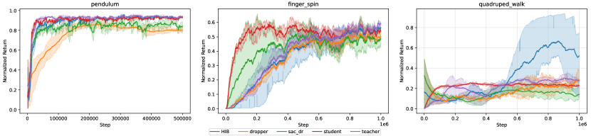
Figure 7: Training curves over three random seeds of HIB compared with other baselines in DMC benchmark

B.2 Details of Legged Robot Benchmark

We create 4096 environment instances to collect data in parallel. In each environment, the robot is initialized with random poses and commanded to walk forward at $v_{x}^{cmd}=0.4m/s$. The robot receives new observations and updates its actions every 0.02 seconds. Similar to Rudin et al. [33], we generate different sets of terrain, including smooth slope, rough slope, stairs up, stairs down, and discrete obstacle, with varying difficulty terrain levels. At training time, the environments are arranged in a $10\times 20$ matrix with each row having terrain of the same type and difficulty increasing from left to right. We train with a curriculum over terrain where robots are first initialized on easy terrain and promoted to harder terrain if they traverse more than half its length. They are demoted to easier terrain if they fail to travel at least half the commanded distance $v_{x}^{cmd}T$ where $T$ is the maximum episode length.

The parameters of dynamic and heights of surroundings are defined as privilege parameters in this environment, as they can only be accessed in simulation but masked in the real world. The Heights of surroundings is an ego-centric map of the terrain around the robot. In particular, it consists of the height values $m_{t}=\{h(x,y)|(x,y)\in P\}$ at 187 points $P=\{-0.8,-0.7,\ldots,0.7,0.8\}\times\{-0.5,-0.4,\ldots,0.4,0.5\}$. And the randomization range of dynamic parameters is shown in Table 6.

Table 6: Privileged knowledge randomization range on Legged Robot Benchmark

Privilege Parameter	Training Range	Testing Range
Friction	[0.5, 1.25]	[0.1, 2.0]
Added mass (kg)	[0, 5]	[0, 7]
$k_{p}$	[45, 65]	[40, 70]
$k_{d}$	[0.7, 0.9]	[0.6, 1.0]

Table 7: Hyperparameters used in HIB

HyperParameter	Value
$\tau$	0.01
update_target_interval	1
$\lambda_{1}$	0.1
$\lambda_{2}$	0.1
history length $k$	50

Appendix C Implementation Details

C.1 Algorithm Implementation

Empirically we find that the learned privilege representation $z_{t}$ is requested to have similar and compact dimensions compared with another policy input $s^{l}_{t}$. So when privileged state $s^{p}_{t}$ is high-dimensional, for example, $s^{p}_{t}$ in Legged Robot benchmark, the encoder $f_{\omega}$ is necessary to project privileged state in a lower dimension, keeping the dimension between $z_{t}$ and $\tilde{e}_{t}$ being the same. In Legged Robot benchmark, the privileged state consists of elevation information and some dynamic parameters, which are noisy and high-dimensional. To project $s^{p}_{t}$ in a lower-dimensional space, encoder $f_{\omega}$ can be a simple two-layer MLP. In the DMC benchmark, encoder $f_{\omega}$ can be an identity operator because the privileged state is defined as dynamic parameters which are compact and have similar dimensions with $s^{l}_{t}$. In this case, $z_{t}$ has the same dimensions as $s^{p}_{t}$ and $\tilde{e}_{t}$.

Considering there is no historical trajectory at the beginning of the episode, we warm up it with zero-padding and then gradually update it for practical implementation. In order to compute HIB loss more accurately, we maintain another IB buffer $\mathcal{B}_{\rm ib}$ to sample $h_{t}$ and $s^{p}_{t}$ practically, which only stores normal trajectories without zero padding.

Our method HIB is sample efficiency compared with the previous two-stage distillation method (i.e., Student) and costs less training time shown in Table 8. As HIB needs more gradient updates, it needs more computation than SAC-DR (or PPO-DR) and Dropper. We use RTX 3080 for both training and evaluation on simulation environments.

Table 8: We report the shortest training time of HIB and other baselines recorded in our experiments.

Domain	SAC-DR (or PPO-DR)	HIB (ours)	Student	Dropper
Pendulum	7.2h	12.0h	12.3h	7.5h
Finger Spin	12.2h	15.2h	15.9h	12.47h
Quadruped Walk	19.8h	25.3h	31.3h	20.5h
Legged Robot (Isaac Gym)	12.1h	15.0h	20.0h	12.7h

C.2 Model Architecture and Hyperparameters

• History encoder $f_{\psi}$ is a TCN model, consisting of three conv1d layers and two linear layers.

• The projector and target projector both have the same architecture, which is a two-layered MLP.

• Encoder $f_{\omega}$ is a two-layer MLP on the Legged Robot Benchmark, and an identical operator on the privileged DMC benchmark.

• Actor-Critic is 3-layered MLPs (with Relu activation).

• Hyperparameters used in HIB can be found in Table 7.

References

- Akhtar and Mian [2018] Naveed Akhtar and Ajmal Mian. Threat of adversarial attacks on deep learning in computer vision: A survey. IEEE Access, 2018. doi: 10.1109/ACCESS.2018.2807385.
- Alemi et al. [2017] Alexander A. Alemi, Ian Fischer, Joshua V. Dillon, and Kevin Murphy. Deep variational information bottleneck. In ICLR, 2017. URL https://openreview.net/forum?id=HyxQzBceg.
- Bai et al. [2021] Chenjia Bai, Lingxiao Wang, Lei Han, Animesh Garg, Jianye Hao, Peng Liu, and Zhaoran Wang. Dynamic bottleneck for robust self-supervised exploration. In Advances in Neural Information Processing Systems, 2021.
- Bai et al. [2018] Shaojie Bai, J Zico Kolter, and Vladlen Koltun. An empirical evaluation of generic convolutional and recurrent networks for sequence modeling. ArXiv, 2018.
- Benjamins et al. [2021] Carolin Benjamins, Theresa Eimer, Frederik Schubert, André Biedenkapp, Bodo Rosenhahn, Frank Hutter, and Marius Lindauer. Carl: A benchmark for contextual and adaptive reinforcement learning. In NeurIPS 2021 Workshop on Ecological Theory of Reinforcement Learning, 2021.
- Chebotar et al. [2019] Yevgen Chebotar, Ankur Handa, Viktor Makoviychuk, Miles Macklin, Jan Issac, Nathan Ratliff, and Dieter Fox. Closing the sim-to-real loop: Adapting simulation randomization with real world experience. In 2019 International Conference on Robotics and Automation (ICRA), 2019.
- Chen et al. [2020] Ting Chen, Simon Kornblith, Mohammad Norouzi, and Geoffrey Hinton. A simple framework for contrastive learning of visual representations. In International conference on machine learning, 2020.
- Chen et al. [2021] Xiaoyu Chen, Jiachen Hu, Chi Jin, Lihong Li, and Liwei Wang. Understanding domain randomization for sim-to-real transfer. In ICLR, 2021.
- Chen and He [2021] Xinlei Chen and Kaiming He. Exploring simple siamese representation learning. In Proceedings of the IEEE/CVF Conference on Computer Vision and Pattern Recognition (CVPR), 2021.
- Eysenbach et al. [2022] Benjamin Eysenbach, Tianjun Zhang, Ruslan Salakhutdinov, and Sergey Levine. Contrastive learning as goal-conditioned reinforcement learning. arXiv, 2022.
- Fan and Li [2022] Jiameng Fan and Wenchao Li. DRIBO: Robust deep reinforcement learning via multi-view information bottleneck. In ICML, 2022.
- Fang et al. [2021] Yuchen Fang, Kan Ren, Weiqing Liu, Dong Zhou, Weinan Zhang, Jiang Bian, Yong Yu, and Tie-Yan Liu. Universal trading for order execution with oracle policy distillation. In Proceedings of the AAAI Conference on Artificial Intelligence, 2021.
- García and Fernández [2015] Javier García and Fernando Fernández. A comprehensive survey on safe reinforcement learning. 2015.
- Grill et al. [2020] Jean-Bastien Grill, Florian Strub, Florent Altché, Corentin Tallec, Pierre Richemond, Elena Buchatskaya, Carl Doersch, Bernardo Avila Pires, Zhaohan Guo, Mohammad Gheshlaghi Azar, Bilal Piot, koray kavukcuoglu, Remi Munos, and Michal Valko. Bootstrap your own latent - a new approach to self-supervised learning. In NeurIPS, 2020.
- Haarnoja et al. [2018] Tuomas Haarnoja, Aurick Zhou, Kristian Hartikainen, George Tucker, Sehoon Ha, Jie Tan, Vikash Kumar, Henry Zhu, Abhishek Gupta, Pieter Abbeel, and Sergey Levine. Soft actor-critic algorithms and applications. CoRR, 2018.
- Hénaff et al. [2020] Olivier J. Hénaff, Aravind Srinivas, Jeffrey De Fauw, Ali Razavi, Carl Doersch, S. M. Ali Eslami, and Aaron Van Den Oord. Data-efficient image recognition with contrastive predictive coding. In Proceedings of the 37th International Conference on Machine Learning, 2020.
- Huynh et al. [2022] Tri Huynh, Simon Kornblith, Matthew R. Walter, Michael Maire, and Maryam Khademi. Boosting contrastive self-supervised learning with false negative cancellation. In 2022 IEEE/CVF Winter Conference on Applications of Computer Vision (WACV), 2022. doi: 10.1109/WACV51458.2022.00106.
- Igl et al. [2018] Maximilian Igl, Luisa Zintgraf, Tuan Anh Le, Frank Wood, and Shimon Whiteson. Deep variational reinforcement learning for pomdps. In International Conference on Machine Learning, pages 2117–2126. PMLR, 2018.
- Jiang et al. [2021] Yifeng Jiang, Tingnan Zhang, Daniel Ho, Yunfei Bai, C. Karen Liu, Sergey Levine, and Jie Tan. Simgan: Hybrid simulator identification for domain adaptation via adversarial reinforcement learning. In 2021 IEEE International Conference on Robotics and Automation (ICRA), 2021. doi: 10.1109/ICRA48506.2021.9561731.
- Kim et al. [2019] Youngjin Kim, Wontae Nam, Hyunwoo Kim, Ji-Hoon Kim, and Gunhee Kim. Curiosity-bottleneck: Exploration by distilling task-specific novelty. In ICML, 2019.
- Kumar et al. [2021] Ashish Kumar, Zipeng Fu, Deepak Pathak, and Jitendra Malik. Rma: Rapid motor adaptation for legged robots. In Robotics: Science and Systems, 2021.
- Lee et al. [2020] Joonho Lee, Jemin Hwangbo, Lorenz Wellhausen, Vladlen Koltun, and Marco Hutter. Learning quadrupedal locomotion over challenging terrain. Science Robotics, 2020.
- Li et al. [2020] Junjie Li, Sotetsu Koyamada, Qiwei Ye, Guoqing Liu, Chao Wang, Ruihan Yang, Li Zhao, Tao Qin, Tie-Yan Liu, and Hsiao-Wuen Hon. Suphx: Mastering mahjong with deep reinforcement learning. CoRR, 2020.
- Lu et al. [2020] Xingyu Lu, Kimin Lee, Pieter Abbeel, and Stas Tiomkin. Dynamics generalization via information bottleneck in deep reinforcement learning. CoRR, 2020.
- Makoviychuk et al. [2021] Viktor Makoviychuk, Lukasz Wawrzyniak, Yunrong Guo, Michelle Lu, Kier Storey, Miles Macklin, David Hoeller, Nikita Rudin, Arthur Allshire, Ankur Handa, and Gavriel State. Isaac gym: High performance gpu-based physics simulation for robot learning. CoRR, 2021.
- Mazoure et al. [2020] Bogdan Mazoure, Remi Tachet des Combes, Thang Long DOAN, Philip Bachman, and R Devon Hjelm. Deep reinforcement and infomax learning. In NeurIPS, 2020.
- Meng et al. [2021] Lingheng Meng, Rob Gorbet, and Dana Kulić. Memory-based deep reinforcement learning for pomdps. In 2021 IEEE/RSJ International Conference on Intelligent Robots and Systems (IROS), pages 5619–5626. IEEE, 2021.
- Miki et al. [2022] Takahiro Miki, Joonho Lee, Jemin Hwangbo, Lorenz Wellhausen, Vladlen Koltun, and Marco Hutter. Learning robust perceptive locomotion for quadrupedal robots in the wild. Science Robotics, 2022.
- Muratore et al. [2020] Fabio Muratore, Christian Eilers, Michael Gienger, and Jan Peters. Bayesian domain randomization for sim-to-real transfer. CoRR, 2020.
- Peng et al. [2018] Xue Bin Peng, Marcin Andrychowicz, Wojciech Zaremba, and Pieter Abbeel. Sim-to-real transfer of robotic control with dynamics randomization. In 2018 IEEE international conference on robotics and automation (ICRA), 2018.
- Poole et al. [2019] Ben Poole, Sherjil Ozair, Aaron Van Den Oord, Alex Alemi, and George Tucker. On variational bounds of mutual information. In ICML, 2019.
- Qiu et al. [2022] Shuang Qiu, Lingxiao Wang, Chenjia Bai, Zhuoran Yang, and Zhaoran Wang. Contrastive ucb: Provably efficient contrastive self-supervised learning in online reinforcement learning. In ICML, 2022.
- Rudin et al. [2022] Nikita Rudin, David Hoeller, Philipp Reist, and Marco Hutter. Learning to walk in minutes using massively parallel deep reinforcement learning. In Conference on Robot Learning, 2022.
- Rusu et al. [2015] Andrei A. Rusu, Sergio Gomez Colmenarejo, Caglar Gulcehre, Guillaume Desjardins, James Kirkpatrick, Razvan Pascanu, Volodymyr Mnih, Koray Kavukcuoglu, and Raia Hadsell. Policy distillation, 2015. URL https://arxiv.org/abs/1511.06295.
- Saxe et al. [2019] Andrew M Saxe, Yamini Bansal, Joel Dapello, Madhu Advani, Artemy Kolchinsky, Brendan D Tracey, and David D Cox. On the information bottleneck theory of deep learning. Journal of Statistical Mechanics: Theory and Experiment, 2019.
- Schulman et al. [2017] John Schulman, Filip Wolski, Prafulla Dhariwal, Alec Radford, and Oleg Klimov. Proximal policy optimization algorithms. CoRR, 2017.
- Schwarzer et al. [2020] Max Schwarzer, Ankesh Anand, Rishab Goel, R. Devon Hjelm, Aaron C. Courville, and Philip Bachman. Data-efficient reinforcement learning with self-predictive representations. In International Conference on Learning Representations, 2020.
- Sermanet et al. [2018] Pierre Sermanet, Corey Lynch, Yevgen Chebotar, Jasmine Hsu, Eric Jang, Stefan Schaal, Sergey Levine, and Google Brain. Time-contrastive networks: Self-supervised learning from video. In 2018 IEEE international conference on robotics and automation (ICRA), 2018.
- Srinivas et al. [2020] A. Srinivas, Michael Laskin, and P. Abbeel. Curl: Contrastive unsupervised representations for reinforcement learning. In International Conference on Machine Learning, 2020.
- Tishby and Zaslavsky [2015] Naftali Tishby and Noga Zaslavsky. Deep learning and the information bottleneck principle. In 2015 ieee information theory workshop (itw), 2015.
- Tishby et al. [2000] Naftali Tishby, Fernando C. Pereira, and William Bialek. The information bottleneck method, 2000. URL https://arxiv.org/abs/physics/0004057.
- Tunyasuvunakool et al. [2020] Saran Tunyasuvunakool, Alistair Muldal, Yotam Doron, Siqi Liu, Steven Bohez, Josh Merel, Tom Erez, Timothy Lillicrap, Nicolas Heess, and Yuval Tassa. dm_control: Software and tasks for continuous control. Software Impacts, 2020.
- Unitree [2022] Unitree. Unitree robotics. https://www.unitree.com/, 2022.
- van den Oord et al. [2018] Aäron van den Oord, Yazhe Li, and Oriol Vinyals. Representation learning with contrastive predictive coding. CoRR, 2018.
- Van der Maaten and Hinton [2008] Laurens Van der Maaten and Geoffrey Hinton. Visualizing data using t-sne. Journal of machine learning research, 2008.
- Wang and Liu [2021] Feng Wang and Huaping Liu. Understanding the behaviour of contrastive loss. In Proceedings of the IEEE/CVF Conference on Computer Vision and Pattern Recognition (CVPR), 2021.
- Xie et al. [2021] Zhaoming Xie, Xingye Da, Michiel van de Panne, Buck Babich, and Animesh Garg. Dynamics randomization revisited: A case study for quadrupedal locomotion. In 2021 IEEE International Conference on Robotics and Automation (ICRA), 2021.
- Yarats et al. [2021] Denis Yarats, Ilya Kostrikov, and Rob Fergus. Image augmentation is all you need: Regularizing deep reinforcement learning from pixels. In ICLR, 2021.
- Zhao et al. [2020a] Wenshuai Zhao, Jorge Peña Queralta, Liu Qingqing, and Tomi Westerlund. Towards closing the sim-to-real gap in collaborative multi-robot deep reinforcement learning. 2020 5th International Conference on Robotics and Automation Engineering (ICRAE), 2020a.
- Zhao et al. [2020b] Wenshuai Zhao, Jorge Peña Queralta, and Tomi Westerlund. Sim-to-real transfer in deep reinforcement learning for robotics: a survey. In 2020 IEEE Symposium Series on Computational Intelligence (SSCI), 2020b.