Conditional Support Alignment for Domain Adaptation with Label Shift

Abstract

Unsupervised domain adaptation (UDA) refers to a domain adaptation framework in which a learning model is trained based on the labeled samples on the source domain and unlabelled ones in the target domain. The dominant existing methods in the field that rely on the classical covariate shift assumption to learn domain-invariant feature representation have yielded suboptimal performance under the label distribution shift between source and target domains. In this paper, we propose a novel conditional adversarial support alignment (CASA) whose aim is to minimize the conditional symmetric support divergence between the source’s and target domain’s feature representation distributions, aiming at a more helpful representation for the classification task. We also introduce a novel theoretical target risk bound, which justifies the merits of aligning the supports of conditional feature distributions compared to the existing marginal support alignment approach in the UDA settings. We then provide a complete training process for learning in which the objective optimization functions are precisely based on the proposed target risk bound. Our empirical results demonstrate that CASA outperforms other state-of-the-art methods on different UDA benchmark tasks under label shift conditions.

1 Introduction

The remarkable success of modern deep learning models often relies on the assumption that training and test data are independent and identically distributed (i.i.d), contrasting the types of real-world problems that can be solved. The violation of that i.i.d. assumption leads to the data distribution shift, or out-of-distribution (OOD) issue, which negatively affects the generalization performance of the learning models (Torralba and Efros, 2011; Li et al., 2017) and renders them impracticable. One of the most popular settings for the OOD problem is unsupervised domain adaptation (UDA) (Ganin and Lempitsky, 2015; David et al., 2010) in which the training process is based on fully-labeled samples from a source domain and completely-unlabeled samples from a target domain, aiming for a good generalization performance on the unseen target data.

While the covariate shift assumption has been extensively studied under the UDA problem setting, with reducing the feature distribution divergence between domains as the dominant approach  (Ganin and Lempitsky, 2015; Tzeng et al., 2017; Shen et al., 2018; Courty et al., 2017; Liu et al., 2019; Long et al., 2015, 2017, 2016, 2014), the label shift assumption ($p(y)$ varies between domains, while $p(x|y)$ is unchanged) remains vastly underexplored in comparison. Compared to the covariate shift assumption, the label shift assumption is often more reasonable in several real-world settings, e.g., the healthcare industry, where the distribution of diseases in medical diagnosis may change across hospitals, while the conditional distribution of symptoms given diseases remains unchanged. In the presence of such label shift,  Zhao et al. (2019); Tachet des Combes et al. (2020) introduced upper bounds on the performance of existing methods and showed that enforcing domain-invariance of learned representation can provably affect generalization performance.

Several UDA methods that explicitly consider the label shift assumption often rely on estimating the importance weights of the source and target label distribution and strictly require the conditional distributions $p(x|y)$ or $p(z|y)$ to be domain-invariant Lipton et al. (2018); Tachet des Combes et al. (2020); Azizzadenesheli et al. (2019). Another popular UDA under label shift framework is enforcing domain invariance of representation $z$ w.r.t some relaxed divergences Wu et al. (2019); Tong et al. (2022).  Wu et al. (2019) proposed reducing $\beta$-admissible distribution divergence to prevent cross-label mapping in conventional domain-invariant approaches. However, choosing inappropriate $\beta$ values can critically reduce the performance of this method under extreme label shifts (Wu et al., 2019; Li et al., 2020).

This paper aims to develop a new theoretically sound approach for UDA under the label shift. Our method is relatively related to but different from the adversarial support alignment (ASA) (Tong et al., 2022) method, which utilizes the symmetric support divergence (SSD) to align the support of the marginal feature distribution of the source and the target domains and achieve impressive domain adaptation results under severe label shift. However, one of the critical drawbacks of the ASA method is that reducing the marginal support divergence indiscriminately may make the learned representation susceptible to conditional distribution misalignment. We illustrate this observation intuitively in Figure 1. Furthermore, the results in Tong et al. (2022) have not been verified rigorously due to the lack of a theoretical guarantee for classification performance in the target domain. We theoretically verify the benefit of our proposed method by introducing a novel generalization error bound for the learning process based on a new conditional SSD.

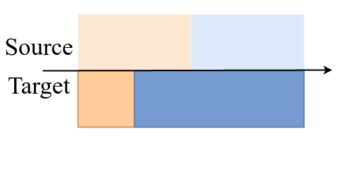
(a) Distribution alignment

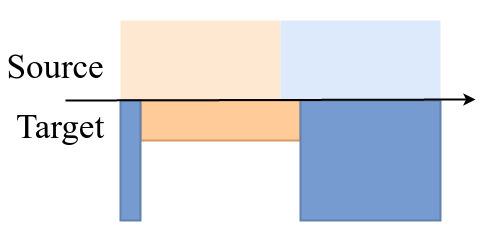
(b) Support alignment

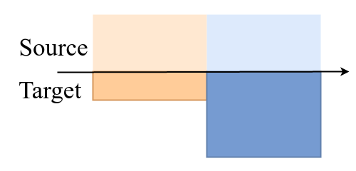
(c) Conditional support alignment

Figure 1: Illustration of the learned latent space of different domain-invariant frameworks under label shift for a binary classification problem. It can be seen that support alignment can mitigate the high error rate induced by distribution alignment, whereas conditional support alignment can achieve the best representation by explicitly aligning the supports of class-conditioned latent distributions.

The main contributions of our paper are summarized as follows:

• We propose a novel conditional adversarial support alignment (CASA) to align the support of the conditional feature distributions on the source and target domains, aiming for a more label-informative representation for the classification task.

• We provide a new theoretical upper bound for the target risk for the learning process of our CASA. We then introduce a complete training scheme for our proposed CASA by minimizing that bound.

• We provide experimental results on several benchmark tasks in UDA, which consistently demonstrate the empirical benefits of our proposed method compared to other relevant existing UDA approaches.

2 Methodology

2.1 Problem Statement

Let us consider a classification framework where $\mathcal{X}\subset\mathbb{R}^{d}$ represents the input space and $\mathcal{Y}=\{y_{1},y_{2},\dots,y_{K}\}$ denotes the output space consisting of $K$ classes. The classes are represented by one-hot vectors $y_{k}$ in $\mathbb{R}^{K}$. A domain is then defined by $P(x,y)\in\mathcal{P}_{\mathcal{X}\times\mathcal{Y}}$, where $\mathcal{P}_{\mathcal{X}\times\mathcal{Y}}$ is the set of joint probability distributions on $\mathcal{X}\times\mathcal{Y}$. The set of conditional distributions of $x$ given $y$, $P(x|y)$, is denoted as $\mathcal{P}_{\mathcal{X}|\mathcal{Y}}$, and the set of probability marginal distributions on $\mathcal{X}$ and $\mathcal{Y}$ is denoted as $\mathcal{P}_{\mathcal{X}}$ and $\mathcal{P}_{\mathcal{Y}}$, respectively. We also denote $P_{X|Y=y_{k}}$ as $P_{X|k}$ for convenience.

Consider an UDA framework, in which the source domain $D^{S}=\left\{\left(x_{i}^{S},y_{i}^{S}\right)\right\}_{i=1}^{n_{S}}$, where $\left(x_{i}^{S},y_{i}^{S}\right)\sim P^{S}(x,y)$, and $y_{i}^{S}\sim P^{S}(y)$; and the target domain $D^{T}=\left\{x_{j}^{T}\right\}_{j=1}^{n_{T}}$, where $x_{j}^{t}\sim P^{T}_{X}\subset\mathcal{P}_{\mathcal{X}}$. Without loss of generality, we assume that both the source and target domains consists of $K$ classes, i.e., $\mathcal{Y}=\{y_{1},\dots,y_{K}\}$. In this paper, we focus on the UDA setting with label shift, which assumes that $P^{S}(y)\neq P^{T}(y)$ while the conditional distributions $P^{S}(x|y)$ and $P^{T}(x|y)$ remain unchanged. Nevertheless, unlike relevant works such as Tachet des Combes et al. (2020); Lipton et al. (2018), we do not make the strong assumption about the invariance of the conditional input distribution $P(x|y)$ or conditional feature distribution $P(z|y)$ between those domains.

A classifier (or hypothesis) is defined by a function $:\mathcal{X}\mapsto\Delta_{K}$, where $\Delta_{K}=\left\{\boldsymbol{\pi}\in\mathbb{R}^{K}:\|\boldsymbol{\pi}\|_{1}=1\wedge\pi\geq\mathbf{0}\right\}$ is the $K$-simplex, and an induced scoring function $g:\mathcal{X}\mapsto\mathbb{R}^{K}$. Consider a loss function $\ell:\mathbb{R}^{K}\times\mathbb{R}^{K}\rightarrow\mathbb{R}_{+}$, satisfying $\ell(y,y)=0,\;\forall y\in\mathcal{Y}$. Given a scoring function $g$, we define its associated classifier as $h_{g}$, i.e., $h_{g}(\mathbf{x})=\hat{y}$ with $\hat{y}\in\operatorname{argmin}_{y\in\mathcal{Y}}\ell[g(\mathbf{x}),y]$.

The $\ell$-risk of a scoring function $g$ over a distribution $P_{X\times Y}$ is then defined by $\mathcal{L}_{P}(g):=\mathbb{E}_{(x,y)\sim P}[\ell(g(x),y)]$, and the classification mismatch of $g$ with a classifier $h$ by $\mathcal{L}_{P}(g,h):=\mathbb{E}_{x\sim P_{X}}[\ell(g(x),h(x))]$. For convenience, we denote the source and target risk of scoring function or classifier $g$ as $\mathcal{L}_{S}(g)$ and $\mathcal{L}_{T}(g)$, respectively.

2.2 A target risk bound based on support misalignment

Similar to Ganin et al. (2016), we assume that the hypothesis $g$ can be decomposed as $g=c\circ f$, where $c:\mathcal{X}\rightarrow\mathcal{Y}$ is the classifier and $f:\mathcal{X}\rightarrow\mathcal{Z}$ is the feature extractor. Here, $\mathcal{Z}$ represents the latent space. Let us denote the domain discriminator as $r:\mathcal{Z}\rightarrow\{0,1\}$, and the probability marginal distribution of latent variable $Z\in\mathcal{Z}$ induced by the source and target domains as $P^{S}_{Z}$ and $P^{T}_{Z}$, respectively.

We next introduce an existing upper bound for the target risk $\mathcal{L}$ based on the support alignment-based divergence between $P^{S}_{Z}$ and $P^{T}_{Z}$. The bound is different from those in previous domain-invariant works, which rely on several types of divergence such as $\mathcal{H}\Delta\mathcal{H}$-divergence (Ben-David et al., 2010), Wasserstein distance (Courty et al., 2017) or maximum mean discrepancy (MMD) (Long et al., 2015).

Definition 1 (Source-guided uncertainty (Dhouib and Maghsudi, 2022)).

Let $\mathbb{H}$ be a hypothesis space, and let $\ell$ be a loss function, and $\mathcal{L}_{P}(\cdot)$ as the associated risk for a distribution $P$. The source-guided uncertainty (or source-conditioned confidence) of a function $g\in\mathbb{H}$ associated with $\ell$ is defined by:

$$\mathcal{C}_{\mathbb{H}}(g)=\inf_{h\in\mathbb{H}}\mathcal{L}_{T}(g,h)+\mathcal{L}_{S}(h),$$ (1)

where $\mathcal{L}_{T}(g,h)$ is the classification mismatch of $g$ and $h$ on $P^{T}_{X}$.

Remark 1.

One important property of the source-guided uncertainty is that if $h_{g}\in\mathbb{H}$, then we have $\mathcal{C}_{\mathbb{H}}(g)\leq\mathcal{L}_{T}(g,h_{g})+\mathcal{L}_{S}(h_{g})$. Dhouib and Maghsudi (2022) showed that when $g(x)$ is in the $K$-dimensional probability simplex, and $\ell$ is the cross entropy loss, then $\mathcal{L}_{T}(g,h_{g})$ is upper-bounded by the average entropy $g(x)$ i.e. $\mathcal{L}_{T}(g,h_{g})\leq E_{x\sim P^{T}_{X}}H(g(x))$, where $H(g)$ denotes the entropy of the function $g$. Hence, minimizing the conditional entropy of predictor $g(x)$ on the target domain, which has been performed in previous domain adaptation algorithms (Shu et al., 2018; Kirchmeyer et al., 2022; Saito et al., 2019; Tong et al., 2022), and the source risk $\mathcal{L}_{S}(h_{g})$ effectively minimizes the source-guided uncertainty $\mathcal{C}_{\mathbb{H}}(g)$.

To derive a target error bound for the marginal support alignment approach (Dhouib and Maghsudi, 2022), we restate the following definition.

Definition 2 (Integral measure discrepancy).

Let $\mathbb{F}$ be a family of nonnegative functions over $\mathbb{X}$, containing the null function. The Integral Measure Discrepancy (IMD) associated to $\mathbb{F}$ between two distribution $\mathcal{Q}$ and $\mathcal{P}$ over $\mathbb{X}$ is

$$\operatorname{IMD}_{\mathbb{F}}\left(\mathcal{Q},\mathcal{P}\right):=\sup_{f\in\mathbb{F}}\int f\mathrm{~{}d}\mathcal{Q}-\int f\mathrm{~{}d}\mathcal{P}.$$ (2)

Intuitively, this discrepancy aims to capture the distances between measures w.r.t. difference masses.

Now, we recapitulate the IMD-based domain adaptation bound in Dhouib and Maghsudi (2022).

Proposition 1 (Domain adaptation bound using IMD Dhouib and Maghsudi (2022)).

Let $\mathbb{H}$ be a hypothesis space, $g$ be a score function, and $\ell$ be a loss function satisfying the triangle inequality. Consider the localized hypothesis $\mathbb{H}^{r}\coloneqq\{h\in\mathbb{H};\mathcal{L}_{S}(h)\leq r\}$ and localized nonnegative function set $\mathbb{F}_{\epsilon}=\{f;f(z)\geq 0,\mathbb{E}_{P^{S}_{Z}}[f]\leq\epsilon\}$. Then, for any $r_{1},r_{2}\geq 0$, we have

$$\mathcal{L}_{T}(g)\leq\mathcal{C}_{\mathbb{H}^{r_{1}}}(g)+\operatorname{IMD}_{\mathbb{F}_{r_{1}+r_{2}}}(P^{T}_{Z},P^{S}_{Z})+\inf_{h\in\mathbb{H}^{r_{2}}}\mathcal{L}_{T}(h)+\mathcal{L}_{S}(h).$$ (3)

By incorporating the Lipschitz property into the functions $f\in\mathbb{F}$,  Dhouib and Maghsudi (2022) demonstrated that the bound presented in Proposition 1 can justify the optimization objective in Tong et al. (2022) using the following divergence.

Definition 3 (Symmetric support divergence).

Assuming that $d$ is a proper distance on the latent space $\mathcal{Z}$. The symmetric support divergence (SSD) between two probability distributions $P_{Z}$ and $Q_{Z}$ is then defined by:

$$\mathcal{D}_{\operatorname{supp}}(P_{Z},Q_{Z})=\mathbb{E}_{z\sim P_{Z}}[d(z,\operatorname{supp}(Q_{Z}))]+\mathbb{E}_{z\sim Q_{Z}}[d(z,\operatorname{supp}(P_{Z}))],$$

where $\operatorname{supp}(P_{Z})$ and $\operatorname{supp}(Q_{Z})$ are the corresponding supports of $P_{Z}$ and $Q_{Z}$, respectively.

Unlike the work in Dhouib and Maghsudi (2022) that extends the bound with $\beta$-admissible distances, our proposed method goes beyond interpreting the bound solely in terms of support divergences Tong et al. (2022). In particular, our method also incorporates the label structures of the domains, allowing a more comprehensive analysis of the underlying relationships.

2.3 A novel conditional SSD-based domain adaptation bound

In this work, we first introduce a definition for a novel conditional symmetric support divergence between the conditional distributions ${P}^{S}_{\ Z|Y}$ and ${P}^{T}_{Z|Y}$. For simplicity, we also denote $d$ as a well-defined distance on the conditional $\mathcal{Z}|\mathcal{Y}$ space.

Definition 4 (Conditional symmetric support divergence).

The conditional symmetric support divergence (CSSD) between the conditional distributions $P^{S}_{Z|Y}$ and $P^{T}_{Z|Y}$ is defined by

$$\mathcal{D}^{c}_{\operatorname{supp}}(P^{S}_{Z|Y},P^{T}_{Z|Y})$$

$$= \sum_{y\in\mathcal{Y}}{P^{S}(Y=y)}\mathbb{E}_{z\sim P^{S}_{Z|Y=y}}[d(z,\operatorname{supp}(P^{T}_{Z|Y=y}))]+{P^{T}(Y=y)}\mathbb{E}_{z\sim P^{T}_{Z|Y=y}}[d(z,\operatorname{supp}(P^{S}_{Z|Y=y}))].$$

In comparison to the SSD in Definition 3, our CSSD takes into account the class proportions in both source and target domains. As a result, the localized IMD considers per-class localized functions, which are defined as the $(\boldsymbol{\epsilon},P^{S}_{Z|Y})$-localized nonnegative function denoted by $\mathbb{F}_{\boldsymbol{\epsilon}}$. Specifically, $\mathbb{F}_{\boldsymbol{\epsilon}}=\{f;f(z)\geq 0,\mathbb{E}_{P^{S}_{Z|k}}[f]\leq\epsilon_{k},\quad k=1\dots K\}$ with $\boldsymbol{\epsilon}=(\epsilon_{1},\dots,\epsilon_{K})\geq 0$.

In the following lemma, we introduce upper bounds for the IMD using CSSD (the corresponding proof is provided in the Appendix).

Lemma 1 (Upper bound IMD using CSSD).

Let $\mathbb{F}$ be a set of nonnegative and $1$-Lipschitz functions, and let $\mathbb{F}_{\boldsymbol{\epsilon}}$ be a $(\boldsymbol{\epsilon},P^{S}_{Z|Y})$-localized nonnegative function. Then, we can bound the IMD w.r.t the conditional support domain and CSSD, respectively, as

$$\operatorname{IMD}_{\mathbb{F}_{\boldsymbol{\epsilon}}}(P^{T}_{Z},P^{S}_{Z}) \leq\sum_{k=1}^{K}q_{k}\mathbb{E}_{z\sim P^{T}_{Z|k}}[d(z,\operatorname{supp}(P^{S}_{Z|k}))]+q_{k}\delta_{k}+p_{k}\epsilon_{k},$$ (4)

$$\operatorname{IMD}_{\mathbb{F}_{\boldsymbol{\epsilon}}}(P^{T}_{Z},P^{S}_{Z}) \leq\mathcal{D}^{c}_{\operatorname{supp}}(P^{T}_{Z|Y},P^{S}_{Z|Y})+\sum_{k=1}^{K}p_{k}\delta_{k}+q_{k}\gamma_{k},$$ (5)

where $\delta_{k}\coloneqq\sup_{z\in\operatorname{supp}P^{S}_{Z|k},f\in\mathbb{F}_{\boldsymbol{\epsilon}}}f(z)$, $\gamma_{k}\coloneqq\sup_{z\in\operatorname{supp}P^{T}_{Z|k},f\in\mathbb{F}_{\boldsymbol{\epsilon}}}f(z)$, $p_{k}=P^{S}(Y=y_{k})$ and $q_{k}=P^{T}(Y=y_{k})$.

We now provide a novel upper bound of the target risk based on CSSD in the following theorem, which is the straightforward result from Lemma 1.

Theorem 1 (Domain adaptation bound via CSSD).

Let $\mathbb{H}$ be a hypothesis space, $g$ be a score function, and $\ell$ be a loss function satisfying the triangle inequality. Consider the localized hypothesis $\mathbb{H}^{\mathbf{r}}\coloneqq\{h\in\mathbb{H};\mathcal{L}_{S_{k}}(h)\leq r_{k},k=1\dots K\}$. Given that all the assumptions for $\mathbb{F}_{\boldsymbol{\epsilon}}$ in Lemma 1 are fulfilled. Then, for any $\mathbf{r}^{1}=(r^{1}_{1},\dots,r^{1}_{K})\geq 0,\mathbf{r}^{2}=(r^{2}_{1},\dots,r^{2}_{K})\geq 0$ that satisfy $r^{1}_{k}+r^{2}_{k}=\epsilon_{k}$, we have:

$$\mathcal{L}_{T}(g)\leq\mathcal{C}_{\mathbb{H}^{\mathbf{r}^{1}}}(g)+\mathcal{D}^{c}_{\operatorname{supp}}(P^{T}_{Z|Y},P^{S}_{Z|Y})+\sum_{k=1}^{K}q_{k}\delta_{k}+p_{k}\gamma_{k}+\inf_{h\in\mathbb{H}^{\mathbf{r}^{2}}}\mathcal{L}_{S}(h)+\mathcal{L}_{T}(h).$$ (6)

Remark 2.

In the case that we do not incorporate the label information, the IMD can be bounded as

$$\operatorname{IMD}_{\mathbb{F}_{\epsilon}}\leq\mathbb{E}_{z\sim P^{T}_{Z}}[d(z,\operatorname{supp}(P^{S}_{Z}))]+\delta+\epsilon,$$ (7)

where $\delta=\sup_{z\in\operatorname{supp}(P^{S}_{Z}),f\in\mathbb{F}_{\epsilon}}f(z)$. Similar to the findings in Dhouib and Maghsudi (2022), the inequality in Equation (7) provides a justification for minimizing SSD proposed in Tong et al. (2022). Notably, this inequality extends to the case where $\epsilon\geq 0$, and thus recover the bound with SSD in Dhouib and Maghsudi (2022) as a special case. Note that in order to make a fair comparison between Equation (4) and (7), we assume that $\sum_{k}\epsilon_{k}p_{k}=\epsilon$ making $\mathbb{F}_{\boldsymbol{\epsilon}}\subseteq\mathbb{F}_{\epsilon}$.

In comparison the the upper bound in Equation  (7), our expectation

$$\sum_{k}q_{k}\mathbb{E}_{z\sim P^{T}_{Z|k}}[d(z,\operatorname{supp}(P^{S}_{Z|k}))]\geq\mathbb{E}_{z\sim P^{T}_{Z}}[d(z,\operatorname{supp}(P^{S}_{Z}))],$$

due to the fact that $d(z,\operatorname{supp}(P^{S}_{Z|k}))\geq d(z,\operatorname{supp}(P^{S}_{Z}))$ and that Jensen’s inequality holds.

However, this inequality does not imply that our bound is less tight than the bound using SSD. When considering the remaining part, we can observe that $\sum_{k}q_{k}\delta_{k}\leq\delta$ since $\operatorname{supp}(P^{S}_{Z|k})\subseteq\operatorname{supp}(P^{S}_{Z})$ for any $k=1,\dots,K$. In other words, there is a trade-off between the distance to support space and the uniform norm (sup norm) of function on the supports.

Remark 3.

The proposed bound shares several similarities with other target error bounds in the UDA literature (Ben-David et al., 2010; Acuna et al., 2021). In particular, these bounds all upperbound the target risk with a source risk term, a domain divergence term, and an ideal joint risk term. The main difference is that we use the conditional symmetric support divergence instead of $\mathcal{H}\Delta\mathcal{H}$-divergence in Ben-David et al. (2010) and $f$-divergence in Acuna et al. (2021), making our bound more suitable for problems with large degrees of label shift, as a lower value of CSSD does not necessarily increase the target risk under large label shift, unlike $\mathcal{H}\Delta\mathcal{H}$-divergence and $f$-divergence Tachet des Combes et al. (2020); Zhao et al. (2019). This is intuitively illustrated by Figure 1 and also empirically validated by experiment results in Section 3.

Furthermore, the localized hypothesis spaces $\mathbb{H}^{\mathbf{r}^{1}}$ and $\mathbb{H}^{\mathbf{r}^{2}}$ are reminiscent of the localized adaptation bound proposed in Zhang et al. (2020). While lower values of $\mathbf{r}^{1},\mathbf{r}^{2}$ can make the term $\sum_{k=1}^{K}q_{k}\delta_{k}+p_{k}\gamma_{k}$ smaller, the source-guided uncertainty term and ideal joint risk term can increase as a result. In our final optimization procedure, we assume the ideal joint risk term and $\sum_{k=1}^{K}q_{k}\delta_{k}+p_{k}\gamma_{k}$ values to be small and minimize the source-guided uncertainty (see section 2.4.1) and CSSD via another proxy (see section 2.4.3) to reduce the target domain risk.

2.4 Training scheme for our CASA

Based on our theoretical guarantee in Theorem 1, we propose Conditional Adversarial Support Alignment (CASA ) algorithm for UDA problem setting under label shift. The main motivation CASA is to minimize both of the source-guided uncertainty $\mathcal{C}_{\mathbb{H}^{\mathbf{r}_{1}}}(g)$ and the CSSD $\mathcal{D}^{c}_{\operatorname{supp}}(P^{T}_{Z|Y},P^{S}_{Z|Y})$ of Eq. (6).

2.4.1 Minimizing source-guided uncertainty

As stated in Remark 1, minimizing the source risk and the target conditional entropy effectively reduces the source-guided uncertainty $\mathcal{C}_{\mathbb{H}^{\mathbf{r}_{1}}}(g)$, which is the second term in the target risk bound of Eq. (6). Minimizing the prediction entropy has also been extensively studied and resulted in many effective semi-supervised (Laine and Aila, 2017; Dai et al., 2017; Tarvainen and Valpola, 2017; Grandvalet and Bengio, 2004), and UDA algorithms (Shu et al., 2018; Kirchmeyer et al., 2022; Liang et al., 2021). Hence, the total loss of CASA first includes classification loss $\ell_{cls}$ on source samples and the conditional entropy loss on target samples defined as follows:

$$\mathcal{L}_{y}(g)=\frac{1}{n_{S}}\sum_{i=1}^{n_{S}}\ell_{cls}(g(x_{i}^{S}),y_{i}^{S})\quad\text{and}\quad\mathcal{L}_{ce}(g)=-\frac{1}{n_{T}}\sum_{i=1}^{n_{T}}g(x_{i}^{T})^{\top}\ln g(x_{i}^{T}).$$

2.4.2 Enforcing Lipschitz hypothesis

The risk bound in Eq. (6) suggests regularizing the Lipschitz continuity of the classifier $c$. Inspired by the success of virtual adversarial training by Miyato et al. (2018) on domain adaptation tasks (Shu et al., 2018; Tong et al., 2022), we instead enforce the locally-Lipschitz constraint of the classifier, which is a relaxation of the global Lipschitz constraint, by enforcing consistency in the norm-ball w.r.t each representation sample $z$. We observe that enforcing the local Lipschitz constraint of $g=c\circ f$ instead of $c$ leads to better performance in empirical experiments, which may suggest the benefit of ensuring Lipschitz continuity of the feature representation function $f$ (Wu et al., 2019; Shu et al., 2018) in addition to the feature classifier $c$. Hence, the following term is added to the overall loss:

$$\mathcal{L}_{v}(c,f)=\frac{1}{n_{S}}\sum_{i=1}^{n_{S}}\max_{\|r\|<\epsilon}\mathrm{D}_{\mathrm{KL}}\left(g(x^{S}_{i})\|g(x^{S}_{i}+r)\right)+\frac{1}{n_{T}}\sum_{i=1}^{n_{T}}\max_{\|r\|<\epsilon}\mathrm{D}_{\mathrm{KL}}\left(g(x^{T}_{i})\|g(x^{T}_{i}+r)\right).$$ (8)

2.4.3 Minimizing conditional symmetric support divergence

The next natural step for tightening the target risk bound in Eq. (6) is to minimize $\mathcal{D}_{\operatorname{supp}}^{c}(P^{S}_{Z|Y},P^{T}_{Z|Y})$. However, it is challenging to directly optimize this term since, in a UDA setting, we have no access to the labels of the target samples. Motivated by the use of pseudo-labels to guide the training process in domain adaptation literature (French et al., 2018; Chen et al., 2019; Long et al., 2018; Zhang et al., 2019a), we alternatively consider minimizing $\mathcal{D}^{c}_{\operatorname{supp}}(P^{S}_{Z|\widehat{Y}},P^{T}_{Z|\widehat{Y}})$ as a proxy for minimizing $\mathcal{D}^{c}_{\operatorname{supp}}(P^{S}_{Z|Y},P^{T}_{Z|Y})$, with $\widehat{Y}$ as pseudo-labels. To mitigate the error accumulation issue of using pseudolabels under large domain shift (Zhang et al., 2019a; Liu et al., 2021), we employ the entropy conditioning technique in Long et al. (2018) in our implementation of CASA .

The next proposition demonstrates that the support divergence between the joint distributions $P^{S}_{Z,Y},P^{T}_{Z,Y}$ can be used to estimate $\mathcal{D}_{\operatorname{supp}}^{c}(P^{S}_{Z|Y},P^{T}_{Z|Y})$.

Proposition 2.

Assuming that $P^{S}(\widehat{Y}=y)>0$, $P^{T}(\widehat{Y}=y)>0\ \forall y\in\mathcal{Y}$, and there exists a well-defined distance denoted by $d$ in the space $\mathcal{Z}\times\mathcal{Y}$. Then $\mathcal{D}^{c}_{\operatorname{supp}}(P^{S}_{Z|Y},P^{T}_{Z|Y})=0$ if and only if $\mathcal{D}_{\operatorname{supp}}(P^{S}_{Z,\widehat{Y}},P^{T}_{Z,\widehat{Y}})=0$.

Proposition 2 motivates us to alternatively minimize the joint support divergence $\mathcal{D}_{\operatorname{supp}}(P^{S}_{Z,\widehat{Y}},P^{T}_{Z,\widehat{Y}})$ to tighten the target error bound, without using any explicit estimate of the marginal label distribution shift as performed in Lipton et al. (2018); Tachet des Combes et al. (2020). Moreover, minimizing this joint support divergence can be performed efficiently in one-dimensional space. In particular, Tong et al. (2022) indicated that when considering the log-loss discriminator $r:\mathcal{X}\rightarrow[0,1]$ trained to discriminate between two distributions $P$ and $Q$ with binary cross entropy loss function can be can be used to estimate $\mathcal{D}_{\operatorname{supp}}(p,q)$.

Exploiting this result, we can align the support of $P^{S}_{Z,\widehat{Y}}$ and $P^{T}_{Z,\widehat{Y}}$ with the optimal discriminator $r^{*}$ that is trained to discriminate between these distributions, which are represented as the outer product $Z\otimes\widehat{Y}$, similar to Long et al. (2018). Consequently, our model incorporates the domain discriminator loss and support alignment loss to minimize the conditional support divergence $\mathcal{D}_{\operatorname{supp}}^{c}(P_{Z|Y},Q_{Z|Y})$ in the error bound specified in Eq. (6).

$$\mathcal{L}_{d}(r) =-\frac{1}{n_{S}}\sum_{i=1}^{n_{S}}\ln\left[r(s(x_{i}^{S}))\right]-\frac{1}{n_{T}}\sum_{i=1}^{n_{T}}\ln\left[1-r(s(x_{i}^{T}))\right];$$ (9)

$$\mathcal{L}_{align}(f) =\frac{1}{n_{S}}\sum_{i=1}^{n_{S}}d\left(r(s(x_{i}^{S})),\{r(s(x_{j}^{T}))\}_{j=1}^{n_{T}}\right)+\frac{1}{n_{T}}\sum_{i=1}^{n_{T}}d\left(r(s(x_{i}^{T})),\{r(s(x_{j}^{S}))\}_{j=1}^{n_{S}}\right),$$ (10)

where $s(x)=f(x)\otimes g(x)$ and $\ u\otimes v=uv^{T}$.

Overall, the training process of our proposed algorithm, CASA , can be formulated as an alternating optimization problem (see Algorithm 1), where $\lambda_{align},\lambda_{y},\lambda_{ce},\lambda_{v}$ are the weight hyper-parameters associated with the respective loss terms:

$$\min_{f,c}\mathcal{L}_{y}(g)+\lambda_{align} \mathcal{L}_{align}(f)+\lambda_{ce}\mathcal{L}_{ce}(g)+\lambda_{v}\mathcal{L}_{v}(g),$$ (11)

$$\min_{r}\mathcal{L}_{d}(r).$$ (12)

Algorithm 1 Conditional Adversarial Support Alignment

Input: $D^{S}=\left\{\left(x_{i}^{S},y_{i}^{S}\right)\right\}_{i=1}^{n_{S}}$, $D^{T}=\left\{x_{j}^{T}\right\}_{j=1}^{n_{T}}$
Output: Feature extractor $f$, classifier $c$, domain discriminator $r$

1:  for number of training iterations do

2:     Sample minibatch from source $\left\{\left(x_{i}^{S},y_{i}^{S}\right)\right\}_{i=1}^{m}$ and target $\left\{x_{i}^{T}\right\}_{i=1}^{m}$

3:     Update $r$ according to Eq. (12)

4:     Update $f,c$ according to Eq. (11)

5:  end for

3 Experiments

Datasets. We focus on visual domain adaptation tasks and empirically evaluate our proposed algorithm CASA on benchmark UDA datasets USPS $\to$ MNIST, STL $\to$ CIFAR and VisDA-2017. We further conduct experiments on the Office-31 dataset and provide the results in Appendix.

Evaluation setting. To assess CASA ’s robustness to label shift, we adopt the experimental protocol of Garg et al. (2020). We simulate label shift using the Dirichlet distribution, ensuring a balanced label distribution in the source domain and a target domain label distribution ($P^{T}_{Y}(y)$) following $Dir(\alpha)$, with $\alpha$ values of ${10,3.0,1.0,0.5}$. Lower $\alpha$ values indicate more severe label shift. We also include a no label shift setting, denoted as $\alpha=\text{None}$, where both source and target label distributions are balanced. For each method and dataset, we perform 5 runs with varying target label distributions across different levels of label shift and report average per-class accuracy on the target domain’s test set as evaluation metrics.

Baselines. We assess the performance of CASA by comparing it with various existing UDA algorithms, including: No DA (training using solely labeled source samples), DANN (Ganin et al., 2016), CDAN (Long et al., 2018) for aligning conditional feature distribution, VADA (Shu et al., 2018) which combines distribution alignment with enforcing the cluster assumption, IWDAN and IWCDAN (Tachet des Combes et al., 2020) for distribution alignment with importance weighting, sDANN (Wu et al., 2019) for aligning feature distribution with $\beta$-relaxed divergence, ASA (Tong et al., 2022) for aligning support of marginal feature distribution, PCT (Tanwisuth et al., 2021) for aligning class-level feature prototypes, and SENTRY (Prabhu et al., 2021) which optimizes entropy with predictive consistency. Note that IWDAN and IWCDAN rely on importance weighting methods that involve estimating the target label distribution. CDAN, IWCDAN and SENTRY employ target pseudolabels to enhance performance under label shift. Further implementation details are provided in Appendix.

Main results. We report the results on USPS$\to$MNIST, STL$\to$CIFAR and VisDA-2017 in Table 1, 2 and 3 respectively.

Table 1: Per-class average accuracies on USPS$\to$MNIST. Bold and underscore denote the best and second-best methods respectively

Algorithm	$\alpha=$ None	$\alpha=10.0$	$\alpha=3.0$	$\alpha=1.0$	$\alpha=0.5$	AVG
No DA	$73.9\pm 2.4$	$73.8\pm 2.5$	$73.5\pm 2.2$	$73.9\pm 2.3$	$73.8\pm 2.3$	$73.8$
DANN (Ganin and Lempitsky, 2015)	$97.8\pm 1.1$	$96.1\pm 1.0$	$89.6\pm 2.0$	$78.7\pm 2.5$	$71.0\pm 3.3$	$86.6$
CDAN (Long et al., 2018)	$97.9\pm 0.2$	$97.6\pm 0.2$	$93.2\pm 1.9$	$81.7\pm 2.9$	$68.4\pm 3.8$	$87.8$
VADA (Shu et al., 2018)	$\mathbf{98.1}\pm 0.1$	$\mathbf{98.1}\pm 0.1$	$\underline{96.8}\pm 1.1$	$84.9\pm 2.5$	$76.8\pm 3.9$	$90.9$
IWDAN (Tachet des Combes et al., 2020)	$97.5\pm 2.5$	$97.1\pm 3.2$	$90.4\pm 4.2$	$81.3\pm 4.1$	$73.3\pm 4.5$	$87.9$
IWCDAN (Tachet des Combes et al., 2020)	$97.8\pm 2.3$	$97.5\pm 2.0$	$91.4\pm 3.1$	$82.6\pm 2.9$	$73.8\pm 3.6$	$88.7$
sDANN (Wu et al., 2019)	$87.4\pm 0.6$	$90.7\pm 0.7$	$92.1\pm 1.9$	$89.4\pm 2.2$	$85.2\pm 3.4$	$89.0$
ASA (Tong et al., 2022)	$94.1\pm 0.6$	$93.7\pm 0.8$	$94.1\pm 0.2$	$\underline{90.8}\pm 2.2$	$\underline{84.7}\pm 1.1$	$\underline{91.5}$
PCT (Tanwisuth et al., 2021)	$97.4\pm 0.2$	$97.2\pm 0.2$	$94.3\pm 3.6$	$82.3\pm 4.4$	$71.8\pm 4.8$	$88.6$
SENTRY (Prabhu et al., 2021)	$97.5\pm 2.0$	$91.5\pm 1.8$	$91.4\pm 2.2$	$84.7\pm 2.5$	$82.3\pm 3.1$	$89.5$
CASA  (Ours)	$\underline{98.0}\pm 0.1$	$\underline{98.0}\pm 0.2$	$\textbf{97.2}\pm 0.5$	$\textbf{96.7}\pm 0.6$	$\textbf{88.3}\pm 1.7$	95.6

Table 2: Results on STL$\to$CIFAR. Same setup as Table 1

Algorithm	$\alpha=$ None	$\alpha=10.0$	$\alpha=3.0$	$\alpha=1.0$	$\alpha=0.5$	AVG
No DA	$69.9\pm 0.6$	$69.8\pm 0.7$	$69.7\pm 0.3$	$68.8\pm 0.9$	$67.9\pm 1.0$	$69.2$
DANN (Ganin and Lempitsky, 2015)	$75.3\pm 0.3$	$74.3\pm 0.4$	$73.5\pm 0.8$	$70.0\pm 2.1$	$67.1\pm 3.0$	$72.0$
CDAN (Long et al., 2018)	$75.5\pm 0.3$	$74.1\pm 0.3$	$73.5\pm 0.3$	$71.3\pm 1.7$	$67.6\pm 2.9$	$72.4$
VADA (Shu et al., 2018)	$\mathbf{77.1}\pm 0.3$	$75.5\pm 0.4$	$73.8\pm 0.7$	$71.3\pm 1.5$	$68.0\pm 1.0$	$73.1$
IWDAN (Tachet des Combes et al., 2020)	$72.9\pm 0.8$	$72.6\pm 1.0$	$71.8\pm 0.9$	$70.6\pm 1.0$	$69.5\pm 1.1$	$71.5$
IWCDAN (Tachet des Combes et al., 2020)	$72.1\pm 1.0$	$72.0\pm 0.4$	$71.5\pm 0.5$	$71.9\pm 0.7$	$69.9\pm 0.9$	$71.5$
sDANN (Wu et al., 2019)	$72.8\pm 0.4$	$72.0\pm 0.3$	$72.0\pm 0.8$	$71.4\pm 1.1$	$\underline{70.1}\pm 0.9$	$71.7$
ASA (Tong et al., 2022)	$72.7\pm 0.4$	$72.2\pm 0.5$	$72.1\pm 0.8$	$\underline{71.5}\pm 1.0$	$69.8\pm 0.7$	$71.7$
PCT (Tanwisuth et al., 2021)	$75.0\pm 0.2$	$76.1\pm 0.2$	$75.0\pm 0.9$	$70.9\pm 1.6$	$68.3\pm 2.3$	$73.1$
SENTRY (Prabhu et al., 2021)	$76.7\pm 0.5$	$\underline{76.6}\pm 1.3$	$\underline{75.2}\pm 1.2$	$71.2\pm 1.0$	$67.0\pm 1.6$	$\underline{73.3}$
CASA  (Ours)	$\underline{76.9}\pm 0.6$	$\mathbf{76.8}\pm 0.6$	$\mathbf{75.8}\pm 0.5$	$\mathbf{74.2}\pm 1.1$	$\mathbf{71.7}\pm 1.2$	75.1

Table 3: Results on VisDA-2017. Same setup as Table 1

Algorithm	$\alpha=$ None	$\alpha=10.0$	$\alpha=3.0$	$\alpha=1.0$	$\alpha=0.5$	AVG
No DA	$55.6\pm 0.7$	$56.0\pm 0.7$	$55.5\pm 0.8$	$55.2\pm 0.9$	$55.1\pm 0.8$	$55.5$
DANN (Ganin and Lempitsky, 2015)	$\textbf{75.5}\pm 0.4$	$71.3\pm 0.4$	$68.4\pm 1.8$	$62.2\pm 2.2$	$56.4\pm 1.6$	$66.8$
CDAN (Long et al., 2018)	$75.0\pm 0.3$	$72.5\pm 0.4$	$69.8\pm 2.8$	$61.3\pm 2.9$	$56.3\pm 3.1$	$67.0$
VADA (Shu et al., 2018)	$\underline{75.2}\pm 0.9$	$72.3\pm 1.2$	$69.6\pm 1.6$	$59.2\pm 1.8$	$52.6\pm 2.3$	$65.8$
IWDAN (Tachet des Combes et al., 2020)	$74.1\pm 0.9$	$\underline{73.3}\pm 0.9$	$\underline{71.4}\pm 1.1$	$65.3\pm 2.3$	$59.7\pm 2.6$	$\underline{68.8}$
IWCDAN (Tachet des Combes et al., 2020)	$73.5\pm 1.1$	$72.5\pm 0.4$	$69.6\pm 1.9$	$62.9\pm 2.8$	$57.2\pm 3.4$	$67.1$
sDANN (Wu et al., 2019)	$72.8\pm 1.1$	$72.2\pm 1.1$	$71.2\pm 2.3$	$\underline{64.9}\pm 3.3$	$\underline{62.5}\pm 3.1$	$68.7$
ASA (Tong et al., 2022)	$66.4\pm 0.3$	$65.3\pm 1.3$	$64.6\pm 2.1$	$61.7\pm 2.8$	$60.1\pm 2.0$	$63.6$
PCT (Tanwisuth et al., 2021)	$68.2\pm 2.3$	$66.8\pm 2.9$	$65.4\pm 3.1$	$60.5\pm 3.6$	$53.6\pm 3.9$	$63.3$
SENTRY (Prabhu et al., 2021)	$67.5\pm 0.5$	$64.5\pm 1.5$	$57.6\pm 1.7$	$53.4\pm 3.2$	$52.6\pm 3.6$	$59.1$
CASA  (Ours)	$74.3\pm 1.5$	$\textbf{73.4}\pm 1.3$	$\textbf{71.8}\pm 1.3$	$\textbf{66.3}\pm 2.3$	$\textbf{63.2}\pm 2.5$	69.8

Table 4: Ablation study of individual loss terms

$\mathcal{L}_{align}$	$\mathcal{L}_{ce}$	$\mathcal{L}_{v}$	$\alpha=$ None	$\alpha=10.0$	$\alpha=3.0$	$\alpha=1.0$	$\alpha=0.5$	AVG
$\checkmark$			$94.5$	$94.2$	$94.3$	$94.3$	$84.9$	$92.4$
$\checkmark$	$\checkmark$		$97.7$	$97.2$	$96.8$	$96.2$	$87.4$	$95.1$
$\checkmark$	$\checkmark$	$\checkmark$	98.0	98.0	97.2	96.7	88.3	95.6

Among the methods focusing on distribution alignment, such as DANN, CDAN, and VADA, they tend to achieve the highest accuracy scores under $\alpha=\text{None}$. However, their performances degrade significantly as the serverity of label shift increases. For instance, under $\alpha=0.5$ in USPS$\to$MNIST task, DANN and CDAN perform worse than source-only training by 2.8% and 5.4%, respectively.

On the other hand, baseline methods in the third group that explicitly address label distribution shift, such as ASA, sDANN and IWCDAN, often outperform distribution alignment methods under severe label shift ($\alpha\in\{1.0,0.5\}$). However, they fall behind these methods when label shift is mild or nonexistent ($\alpha\in\{\text{None},10.0\}$) by a large margin of 2-4% in the STL$\to$CIFAR task.

In contrast, CASA outperforms baseline methods on 11 out of 15 transfer tasks. It achieves the second-highest average accuracies when there is no label shift in the USPS$\to$MNIST and STL$\to$CIFAR tasks, and outperforms the second-best methods by 3.6%, 1.6% and 0.7% under $\alpha=0.5$ in the USPS$\to$MNIST, STL$\to$CIFAR and VisDA-2017 tasks, respectively. The robustness of CASA to different label shift levels is further demonstrated by its highest average accuracy results, surpassing the second-best methods by 4.1%, 1.8% and 1.0% on the 3 benchmark datasets.

In comparison to IWCDAN, which tries to align the conditional feature distribution also by using pseudo labels, CASA consistently provides higher accuracy across 15 transfer tasks, surpassing IWCDAN by a margin of 3.6% in terms of average accuracy on the STL$\to$CIFAR dataset. We hypothesize that aligning the conditional feature support is more robust to label distribution shift than aligning the conditional feature distribution. On the other hand, the performance of CASA is also consistently higher than that of ASA, which agrees with our theoretical analysis 2 that justifies minimizing CSSD over minimizing SSD.

Analysis of individual loss terms. To study the impact of each loss term in Eq.(11), we provide additional experiment results, which consist of the average accuracy over 5 different random runs on USPS$\to$MNIST in Table 4. It is evident that the conditional support alignment loss term $\mathcal{L}_{align}$, conditional entropy loss term $\mathcal{L}_{ce}$ and virtual adversarial loss term $\mathcal{L}_{v}$ all improve the model’s performance across different levels of label shift.

Visualization of learned feature embeddings under severe label shift. We first conduct an experiment to visualize the effectiveness of our proposed method. Images from three classes (3, 5, and 9) are selected from USPS and MNIST datasets, following Tong et al. (2022), to create source and target domains, respectively. The label probabilities are equal in the source domain, while they are $[22.9\%,64.7\%,12.4\%]$ in the target domain. We compare the per-class accuracy scores, Wasserstein distance $\mathcal{D}_{W}$, $\mathcal{D}^{c}_{\operatorname{supp}}$ and 2D feature distribution of CDAN (Long et al., 2018), ASA (Tong et al., 2022) and CASA.

Fig. 2 shows that CASA achieves a higher target average accuracy, resulting in a clearer separation among classes and more distinct feature clusters compared to CDAN and ASA. Although ASA reduces the overlap of different target classes to some extent, its approach that only enforces support alignment between marginals does not fully eradicate the overlap issue. CASA tackles this drawback by considering discriminative class information during the support alignment in feature embeddings.

The plot also demonstrates that CASA effectively reduces $\mathcal{D}^{c}_{\operatorname{supp}}$ through the proxy objective in Proposition 2. Our observations are consistent with those made in Tong et al. (2022), namely that lower values of $\mathcal{D}^{c}_{\operatorname{supp}}$ tend to correlate with higher accuracy values under label distribution shift. In contrast, this observation is not true for the case of conventional distribution divergence, such as Wasserstein distance.

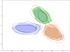
(a)

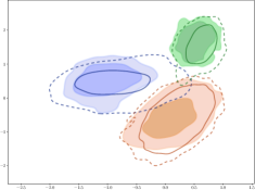
(b)

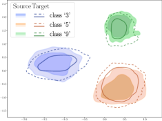
(c)

Figure 2: Visualization of support of feature representations for 3 classes in the USPS $\to$ MNIST task. Similar to Tong et al. (2022), each plot illustrates the 2 level sets of kernel density estimates for both the source and target features. The average accuracy, Wasserstein distance $\mathcal{D}_{W}$ and $\mathcal{D}^{c}_{\operatorname{supp}}$ are also provided.

4 Related works

A dominant approach for tackling the UDA problem is learning domain-invariant feature representation, based on the theory of Ben-David et al. (2006), which suggests minimizing the $\mathcal{H}\Delta\mathcal{H}$-divergence between the two marginal distributions $P^{S}_{Z},P^{T}_{Z}$. More general target risk bound than that of Ben-David et al. (2006) have been developed by extending the problem setting to multi-source domain adaptation (Mansour et al., 2008; Zhao et al., 2018; Phung et al., 2021), or considering discrepancy distance (Mansour et al., 2009), hypothesis-independent disparity discrepancy (Zhang et al., 2019b), or PAC-Bayesian bounds with weighted majority vote learning (Germain et al., 2016).

Numerous methods have been proposed to align the distribution of feature representation between source and target domains, using Wasserstein distance (Courty et al., 2017; Shen et al., 2018; Lee and Raginsky, 2018), maximum mean discrepancy (Long et al., 2014, 2015, 2016), Jensen-Shannon divergence (Ganin and Lempitsky, 2015; Tzeng et al., 2017), or first and second moment of the concerned distribution (Sun and Saenko, 2016; Peng et al., 2019),.

However, recent works have pointed out the limits of enforcing invariant feature representation distribution, particularly when the marginal label distribution differs significantly between domains (Johansson et al., 2019; Zhao et al., 2019; Wu et al., 2019; Tachet des Combes et al., 2020). Based on these theoretical results, different methods have been proposed to tackle UDA under label shift, often by minimizing $\beta$-relaxed Wasserstein distance (Tong et al., 2022; Wu et al., 2019), or estimating the importance weight of label distribution between source and target domains (Lipton et al., 2018; Tachet des Combes et al., 2020; Azizzadenesheli et al., 2019).

Our proposed method leverages the Symmetric Support Divergence proposed by Tong et al. (2022). Different from the work in  Tong et al. (2022) that aims to align the support of marginal feature distributions in source and target domains, the key idea of our proposed method is to tackle the label shift by aligning the conditional distributions of the latent given the label, targeting a label-informative representation. We theoretically justify our proposed method by introducing a novel theoretical target risk bound inspired by the work of Dhouib and Maghsudi (2022).

5 Conclusion

In this paper, we propose a novel CASA framework to handle the UDA problem under label distribution shift. The key idea of our work is to learn a more discriminative and useful representation for the classification task by aligning the supports of the conditional distributions between the source and target domains. We next provide a novel theoretical error bound on the target domain and then introduce a complete training process for our proposed CASA . Our experimental results consistently show that our CASA framework outperforms other relevant UDA baselines on several benchmark tasks. We plan to employ and extend our proposed method to more challenging problem settings, such as domain generalization and universal domain adaptation.

Appendix A Proofs of Our Theory Development

A.1 Lemma  1

Proof.

By the law of total expectation, we can write

$$\operatorname{IMD}_{\mathbb{F}_{\boldsymbol{\epsilon}}}(P^{T}_{Z},P^{S}_{Z})=\sup_{f\in\mathbb{F}_{\boldsymbol{\epsilon}}}\mathbb{E}_{P^{T}_{Y}}\mathbb{E}_{P^{T}_{Z|Y}}[f]-\mathbb{E}_{P^{S}_{Y}}\mathbb{E}_{P^{T}_{Z|Y}}[f]=\sup_{f\in\mathbb{F}_{\boldsymbol{\epsilon}}}\sum_{k=1}^{K}q_{k}\mathbb{E}_{P^{T}_{Z|Y=k}}[f]-p_{k}\mathbb{E}_{P^{S}_{Z|Y=k}}[f].$$

Next, we bound the function $f$ using the assumption that $f$ is $1$-Lipschitz. That is, for any $z\in\mathcal{Z}$ and $z^{\prime}\in\operatorname{supp}P^{S}_{Z|Y=k}$, we have

$$f(z)\leq f(z^{\prime})+d(z,z^{\prime})\leq\delta_{k}+d(z,z^{\prime}).$$

The infimum of $d(z,z^{\prime})$ w.r.t $z^{\prime}\in\operatorname{supp}P^{S}_{Z|Y=k}$ in the right-hand side will result in $d(z,\operatorname{supp}P^{S}_{Z|Y=k})$. Therefore, we have

$$f(z)\leq\delta_{k}+d(z,\operatorname{supp}P^{S}_{Z|Y=k})$$

Now the class-conditioned expectation of $f$ is bounded by

$$\mathbb{E}_{P^{T}_{Z|Y=k}}[f]\leq\delta_{k}+\mathbb{E}_{P^{T}_{Z|Y=k}}[d(z,\operatorname{supp}P^{S}_{Z|Y=k})].$$

Together with the definition of $\mathbb{F}_{\boldsymbol{\epsilon}}$, we can arrive with the first result

$$\operatorname{IMD}_{\mathbb{F}_{\boldsymbol{\epsilon}}}(P^{T}_{Z},P^{S}_{Z})\leq\sum_{k=1}^{K}q_{k}\mathbb{E}_{P^{T}_{Z|Y=k}}[d(z,\operatorname{supp}P^{S}_{Z|Y=k})]+q_{k}\delta_{k}+p_{k}\epsilon_{k}.$$

The second result can be obtained by deriving a similar bound for $\mathbb{E}_{P^{S}_{Z}|Y=k}[f]$ as

$$\mathbb{E}_{P^{S}_{Z|Y=k}}[f]\leq\gamma_{k}+\mathbb{E}_{P^{S}_{Z}|Y=k}[d(z,\operatorname{supp}P^{T}_{Z|Y=k})].$$

∎

A.2 Proposition 2

Proof.

We have $\mathcal{D}_{supp}^{c}(P^{S}_{Z|\widehat{Y}},P^{T}_{Z|\widehat{Y}})=0$ is equivalent to

$$P^{S}(Z=z|\widehat{Y}=y)>0\;\text{iff}\;P^{T}(Z=z|\widehat{Y}=y)>0$$

Since $P^{S}(\widehat{Y}=y)>0$, and $P^{T}(\widehat{Y}=y)>0$, the condition above is equivalent to

$$P^{S}(Z=z,\widehat{Y}=y)>0\;\text{iff}\;P^{T}(Z=z,\widehat{Y}=y)>0,$$

which means that

$$\mathcal{D}_{supp}(P^{S}_{Z,\widehat{Y}},P^{T}_{Z,\widehat{Y}})=0.$$

∎

Appendix B Additional experiment results

We further conduct experiments on Office-31. Given the relatively low number of images per class in this dataset, which is less than 100, simulating label shift using the Dirichlet distribution may significantly reduce the number of training samples available. Instead, we adopt the subsampling protocol in Tanwisuth et al. [2021] and Tachet des Combes et al. [2020], which induces a less severe label distribution shift than that of Dirichlet distribution, and modify the target domains by using only 30% of the first half of their classes for training. Unlike Tanwisuth et al. [2021] and Tachet des Combes et al. [2020], we refrain from altering the label distribution of the source domain since the training data from the source domain is often more easily curated compared to the training data from the target domain Garg et al. [2023]. We take the existing results for baselines with the same subsampling settings and hyper-parameters from Tanwisuth et al. [2021], and perform experiments for additional baselines. Table 5 presents the average accuracy of different methods over 5 random runs, on both the original and subsampled Office-31 dataset. On Office-31 dataset, CASA achieves state-of-the-art result on the subsampled target domain setting, and the second-best result on the original dataset setting.

Table 5: Office-31 results

Algorithm	O-31	sub-T 0-31
No DA	$76.1$	$76.1$
DANN [Ganin and Lempitsky, 2015]	$82.2$	$75.9$
CDAN [Long et al., 2018]	$87.2$	$83.0$
VADA [Shu et al., 2018]	$84.5$	$81.8$
IWDAN [Tachet des Combes et al., 2020]	$83.9$	$79.2$
IWCDAN [Tachet des Combes et al., 2020]	$87.3$	$83.5$
sDANN [Wu et al., 2019]	$81.5$	$80.3$
ASA [Tong et al., 2022]	$79.8$	$79.4$
PCT [Tanwisuth et al., 2021]	88.7	$86.2$
SENTRY [Prabhu et al., 2021]	$83.5$	$82.8$
CASA  (Ours)	$87.8$	86.5

Appendix C Dataset description

• USPS $\to$ MNIST is a digits benchmark for adaptation between two grayscale handwritten digit datasets: USPS [Hull, 1994] and MNIST [LeCun et al., 1998]. In this task, data from the USPS dataset is considered the source domain, while the MNIST dataset is considered the target domain.

• STL $\to$ CIFAR. This task considers the adaptation between two colored image classification datasets: STL [Coates and Ng, 2012] and CIFAR-10 [Krizhevsky et al., 2009]. Both datasets consist of 10 classes of labels. Yet, they only share 9 common classes. Thus, we adapt the 9-class classification problem proposed by Shu et al. [2018] and select subsets of samples from the 9 common classes.

• VisDA-2017 is a synthetic to real images adaptation benchmark of the VisDA-2017 challenge [Peng et al., 2017]. The training domain consists of CAD-rendered 3D models of 12 classes of objects from different angles and under different lighting conditions. We use the validation data of the challenge, which consists of objects of the same 12 classes cropped from images of the MS COCO dataset [Lin et al., 2014], as the target domain.

• Office-31 contains around 5000 images of 31 different object types from 3 domains: Amazon, DSLR and Webcam [Saenko et al., 2010]. The object categories include common office objects such as printer, file cabinets, and monitor.

Appendix D Implementation details

USPS $\to$ MNIST. Following Tachet des Combes et al. [2020], we employ a LeNet-variant [LeCun et al., 1998] with a 500-d output layer as the backbone architecture for the feature extractor. For the discriminator, we implement a 3-layer MLP with 512 hidden units and leaky-ReLU activation.

We train all classifiers, along with their feature extractors and discriminators, using $65000$ SGD steps with learning rate $0.02$, momentum $0.9$, weight decay $5\times 10^{-4}$, and batch size $64$. The discriminator is updated once for every update of the feature extractor and the classifier. After the first $30000$ steps, we apply linear annealing to the learning rate for the next $30000$ steps until it reaches the final value of $2\times 10^{-5}$.

For the loss of the feature extractor, the alignment weight $\lambda_{align}$ is scheduled to linearly increase from $0$ to $1.0$ in the first $10000$ steps for all alignment methods, and $\lambda_{vat}$ equals 1.0 for the source, and 0.1 for the target domains.

STL $\to$ CIFAR. We follow Tong et al. [2022] in using the same deep CNN architecture as the backbone for the feature extractor. The 192-d feature vector is then fed to a single-layer linear classifier. The discriminator is a 3-layer MLP with 512 hidden units and leaky-ReLU activation.

We train all classifiers, along with their feature extractors and discriminators, using $40000$ ADAM [Kingma and Ba, 2015] steps with learning rate $0.001$, $\beta_{1}=0.5$, $\beta_{2}=0.999$, no weight decay, and batch size $64$. The discriminator is updated once for every update of the feature extractor and the classifier.

For the loss of the feature extractor, the weight of the alignment term is set to a constant $\lambda_{align}=0.1$ for all alignment methods. The weight of the auxiliary conditional entropy term is $\lambda_{ce}=0.1$ for all domain adaptation methods, and $\lambda_{vat}$ equals 1.0 for the source, and 0.1 for the target domains.

VisDA-2017. We use a modified ResNet-50 [He et al., 2016] with a 256-d final bottleneck layer as the backbone of our feature extractor. All layers of the backbone, except for the final one, use pretrained weights from torchvision model hub. The classifier is a single linear layer. Similar to other tasks, the discriminator is a 3-layer MLP with 1024 hidden units and leaky-ReLU activation.

We train all classifiers, feature extractors, and discriminators using $25000$ SGD steps with momentum $0.9$, weight decay $0.01$, and batch size $64$. We use a learning rate of $0.001$ for feature extractors. For the classifiers, the learning rate is $0.01$. For the discriminator, the learning rate is $0.005$. We apply linear annealing to the learning rate of feature extractors and classifiers such that their learning rates are decreased by a factor of $0.05$ by the end of training.

The alignment weight $\lambda_{align}$ is scheduled to linearly increase from $0$ to $0.1$ in the first $5000$ steps for all alignment methods. The weight of the auxiliary conditional entropy term is set to a constant $\lambda_{ce}=0.05$, and $\lambda_{vat}$ equals 0 for the source, and 0.1 for the target domains.

Office-31 We use Resnet50 as the backbone feature extractor, and replace the fully-connected layer with a 256-d bottleneck layer. The classifier and discriminator share the same architecture as those of VisDA-2017’s experiments. All methods are trained with $10000$ steps using the SGD optimizer, with momentum of $0.9$, and learning rate of $0.01$ for the classifier and the discriminator, which is ten times larger than that of the feature extractor, and batch size $36$. We also adopt same learning rate scheduler and progressive discriminator training strategy from Junguang Jiang [2020].

References

- Acuna et al. (2021) D. Acuna, G. Zhang, M. T. Law, and S. Fidler. f-domain adversarial learning: Theory and algorithms. In International Conference on Machine Learning, pages 66–75. PMLR, 2021.
- Azizzadenesheli et al. (2019) K. Azizzadenesheli, A. Liu, F. Yang, and A. Anandkumar. Regularized learning for domain adaptation under label shifts. In International Conference on Learning Representations, 2019.
- Ben-David et al. (2006) S. Ben-David, J. Blitzer, K. Crammer, and F. Pereira. Analysis of representations for domain adaptation. Advances in neural information processing systems, 19, 2006.
- Ben-David et al. (2010) S. Ben-David, J. Blitzer, K. Crammer, A. Kulesza, F. Pereira, and J. W. Vaughan. A theory of learning from different domains. Machine learning, 79(1):151–175, 2010.
- Chen et al. (2019) C. Chen, W. Xie, W. Huang, Y. Rong, X. Ding, Y. Huang, T. Xu, and J. Huang. Progressive feature alignment for unsupervised domain adaptation. In Proceedings of the IEEE/CVF conference on computer vision and pattern recognition, pages 627–636, 2019.
- Coates and Ng (2012) A. Coates and A. Y. Ng. Learning feature representations with k-means. In Neural networks: Tricks of the trade, pages 561–580. Springer, 2012.
- Courty et al. (2017) N. Courty, R. Flamary, A. Habrard, and A. Rakotomamonjy. Joint distribution optimal transportation for domain adaptation. Advances in Neural Information Processing Systems, 30, 2017.
- Dai et al. (2017) Z. Dai, Z. Yang, F. Yang, W. W. Cohen, and R. R. Salakhutdinov. Good semi-supervised learning that requires a bad gan. Advances in neural information processing systems, 30, 2017.
- David et al. (2010) S. B. David, T. Lu, T. Luu, and D. Pál. Impossibility theorems for domain adaptation. In Proceedings of the Thirteenth International Conference on Artificial Intelligence and Statistics, pages 129–136. JMLR Workshop and Conference Proceedings, 2010.
- Dhouib and Maghsudi (2022) S. Dhouib and S. Maghsudi. Connecting sufficient conditions for domain adaptation: source-guided uncertainty, relaxed divergences and discrepancy localization. arXiv preprint arXiv:2203.05076, 2022.
- French et al. (2018) G. French, M. Mackiewicz, and M. Fisher. Self-ensembling for visual domain adaptation. In International Conference on Learning Representations, 2018.
- Ganin and Lempitsky (2015) Y. Ganin and V. Lempitsky. Unsupervised domain adaptation by backpropagation. In International conference on machine learning, pages 1180–1189. PMLR, 2015.
- Ganin et al. (2016) Y. Ganin, E. Ustinova, H. Ajakan, P. Germain, H. Larochelle, F. Laviolette, M. Marchand, and V. Lempitsky. Domain-adversarial training of neural networks. The journal of machine learning research, 17(1):2096–2030, 2016.
- Garg et al. (2020) S. Garg, Y. Wu, S. Balakrishnan, and Z. Lipton. A unified view of label shift estimation. Advances in Neural Information Processing Systems, 33:3290–3300, 2020.
- Garg et al. (2023) S. Garg, N. Erickson, J. Sharpnack, A. Smola, S. Balakrishnan, and Z. Lipton. Rlsbench: Domain adaptation under relaxed label shift. arXiv preprint arXiv:2302.03020, 2023.
- Germain et al. (2016) P. Germain, A. Habrard, F. Laviolette, and E. Morvant. A new pac-bayesian perspective on domain adaptation. In International conference on machine learning, pages 859–868. PMLR, 2016.
- Grandvalet and Bengio (2004) Y. Grandvalet and Y. Bengio. Semi-supervised learning by entropy minimization. Advances in neural information processing systems, 17, 2004.
- He et al. (2016) K. He, X. Zhang, S. Ren, and J. Sun. Deep residual learning for image recognition. In Proceedings of the IEEE conference on computer vision and pattern recognition, pages 770–778, 2016.
- Hull (1994) J. J. Hull. A database for handwritten text recognition research. IEEE Transactions on pattern analysis and machine intelligence, 16(5):550–554, 1994.
- Johansson et al. (2019) F. D. Johansson, D. Sontag, and R. Ranganath. Support and invertibility in domain-invariant representations. In The 22nd International Conference on Artificial Intelligence and Statistics, pages 527–536. PMLR, 2019.
- Junguang Jiang (2020) B. F. M. L. Junguang Jiang, Baixu Chen. Transfer-learning-library. https://github.com/thuml/Transfer-Learning-Library, 2020.
- Kingma and Ba (2015) D. P. Kingma and J. Ba. Adam: A method for stochastic optimization. In International Conference on Learning Representations, 2015.
- Kirchmeyer et al. (2022) M. Kirchmeyer, A. Rakotomamonjy, E. de Bezenac, and P. Gallinari. Mapping conditional distributions for domain adaptation under generalized target shift. In International Conference on Learning Representations, 2022.
- Krizhevsky et al. (2009) A. Krizhevsky, G. Hinton, et al. Learning multiple layers of features from tiny images. 2009.
- Laine and Aila (2017) S. Laine and T. Aila. Temporal ensembling for semi-supervised learning. In International Conference on Learning Representations, 2017.
- LeCun et al. (1998) Y. LeCun, L. Bottou, Y. Bengio, and P. Haffner. Gradient-based learning applied to document recognition. Proceedings of the IEEE, 86(11):2278–2324, 1998.
- Lee and Raginsky (2018) J. Lee and M. Raginsky. Minimax statistical learning with wasserstein distances. Advances in Neural Information Processing Systems, 31, 2018.
- Li et al. (2020) B. Li, Y. Wang, T. Che, S. Zhang, S. Zhao, P. Xu, W. Zhou, Y. Bengio, and K. Keutzer. Rethinking distributional matching based domain adaptation. arXiv preprint arXiv:2006.13352, 2020.
- Li et al. (2017) D. Li, Y. Yang, Y.-Z. Song, and T. M. Hospedales. Deeper, broader and artier domain generalization. In Proceedings of the IEEE international conference on computer vision, pages 5542–5550, 2017.
- Liang et al. (2021) J. Liang, D. Hu, Y. Wang, R. He, and J. Feng. Source data-absent unsupervised domain adaptation through hypothesis transfer and labeling transfer. IEEE Transactions on Pattern Analysis and Machine Intelligence, 2021.
- Lin et al. (2014) T.-Y. Lin, M. Maire, S. Belongie, J. Hays, P. Perona, D. Ramanan, P. Dollár, and C. L. Zitnick. Microsoft coco: Common objects in context. In Computer Vision–ECCV 2014: 13th European Conference, Zurich, Switzerland, September 6-12, 2014, Proceedings, Part V 13, pages 740–755. Springer, 2014.
- Lipton et al. (2018) Z. Lipton, Y.-X. Wang, and A. Smola. Detecting and correcting for label shift with black box predictors. In International conference on machine learning, pages 3122–3130. PMLR, 2018.
- Liu et al. (2019) H. Liu, M. Long, J. Wang, and M. Jordan. Transferable adversarial training: A general approach to adapting deep classifiers. In International Conference on Machine Learning, pages 4013–4022. PMLR, 2019.
- Liu et al. (2021) H. Liu, J. Wang, and M. Long. Cycle self-training for domain adaptation. Advances in Neural Information Processing Systems, 34:22968–22981, 2021.
- Long et al. (2014) M. Long, J. Wang, G. Ding, J. Sun, and P. S. Yu. Transfer joint matching for unsupervised domain adaptation. In Proceedings of the IEEE conference on computer vision and pattern recognition, pages 1410–1417, 2014.
- Long et al. (2015) M. Long, Y. Cao, J. Wang, and M. Jordan. Learning transferable features with deep adaptation networks. In International conference on machine learning, pages 97–105. PMLR, 2015.
- Long et al. (2016) M. Long, H. Zhu, J. Wang, and M. I. Jordan. Unsupervised domain adaptation with residual transfer networks. Advances in neural information processing systems, 29, 2016.
- Long et al. (2017) M. Long, H. Zhu, J. Wang, and M. I. Jordan. Deep transfer learning with joint adaptation networks. In International conference on machine learning, pages 2208–2217. PMLR, 2017.
- Long et al. (2018) M. Long, Z. Cao, J. Wang, and M. I. Jordan. Conditional adversarial domain adaptation. Advances in neural information processing systems, 31, 2018.
- Mansour et al. (2008) Y. Mansour, M. Mohri, and A. Rostamizadeh. Domain adaptation with multiple sources. Advances in neural information processing systems, 21, 2008.
- Mansour et al. (2009) Y. Mansour, M. Mohri, and A. Rostamizadeh. Domain adaptation: Learning bounds and algorithms. In Proceedings of The 22nd Annual Conference on Learning Theory (COLT 2009), Montréal, Canada, 2009.
- Miyato et al. (2018) T. Miyato, S.-i. Maeda, M. Koyama, and S. Ishii. Virtual adversarial training: a regularization method for supervised and semi-supervised learning. IEEE transactions on pattern analysis and machine intelligence, 41(8):1979–1993, 2018.
- Peng et al. (2017) X. Peng, B. Usman, N. Kaushik, J. Hoffman, D. Wang, and K. Saenko. Visda: The visual domain adaptation challenge. arXiv preprint arXiv:1710.06924, 2017.
- Peng et al. (2019) X. Peng, Q. Bai, X. Xia, Z. Huang, K. Saenko, and B. Wang. Moment matching for multi-source domain adaptation. In Proceedings of the IEEE/CVF international conference on computer vision, pages 1406–1415, 2019.
- Phung et al. (2021) T. Phung, T. Le, T.-L. Vuong, T. Tran, A. Tran, H. Bui, and D. Phung. On learning domain-invariant representations for transfer learning with multiple sources. Advances in Neural Information Processing Systems, 34, 2021.
- Prabhu et al. (2021) V. Prabhu, S. Khare, D. Kartik, and J. Hoffman. Sentry: Selective entropy optimization via committee consistency for unsupervised domain adaptation. In Proceedings of the IEEE/CVF International Conference on Computer Vision, pages 8558–8567, 2021.
- Saenko et al. (2010) K. Saenko, B. Kulis, M. Fritz, and T. Darrell. Adapting visual category models to new domains. In European conference on computer vision, pages 213–226. Springer, 2010.
- Saito et al. (2019) K. Saito, D. Kim, S. Sclaroff, T. Darrell, and K. Saenko. Semi-supervised domain adaptation via minimax entropy. In Proceedings of the IEEE/CVF International Conference on Computer Vision, pages 8050–8058, 2019.
- Shen et al. (2018) J. Shen, Y. Qu, W. Zhang, and Y. Yu. Wasserstein distance guided representation learning for domain adaptation. In Thirty-second AAAI conference on artificial intelligence, 2018.
- Shu et al. (2018) R. Shu, H. H. Bui, H. Narui, and S. Ermon. A DIRT-T approach to unsupervised domain adaptation. In International Conference on Learning Representations, 2018.
- Sun and Saenko (2016) B. Sun and K. Saenko. Deep coral: Correlation alignment for deep domain adaptation. In European conference on computer vision, pages 443–450. Springer, 2016.
- Tachet des Combes et al. (2020) R. Tachet des Combes, H. Zhao, Y.-X. Wang, and G. J. Gordon. Domain adaptation with conditional distribution matching and generalized label shift. Advances in Neural Information Processing Systems, 33:19276–19289, 2020.
- Tanwisuth et al. (2021) K. Tanwisuth, X. Fan, H. Zheng, S. Zhang, H. Zhang, B. Chen, and M. Zhou. A prototype-oriented framework for unsupervised domain adaptation. Advances in Neural Information Processing Systems, 34:17194–17208, 2021.
- Tarvainen and Valpola (2017) A. Tarvainen and H. Valpola. Mean teachers are better role models: Weight-averaged consistency targets improve semi-supervised deep learning results. Advances in neural information processing systems, 30, 2017.
- Tong et al. (2022) S. Tong, T. Garipov, Y. Zhang, S. Chang, and T. S. Jaakkola. Adversarial support alignment. In International Conference on Learning Representations, 2022.
- Torralba and Efros (2011) A. Torralba and A. A. Efros. Unbiased look at dataset bias. In CVPR 2011, pages 1521–1528. IEEE, 2011.
- Tzeng et al. (2017) E. Tzeng, J. Hoffman, K. Saenko, and T. Darrell. Adversarial discriminative domain adaptation. In Proceedings of the IEEE conference on computer vision and pattern recognition, pages 7167–7176, 2017.
- Wu et al. (2019) Y. Wu, E. Winston, D. Kaushik, and Z. Lipton. Domain adaptation with asymmetrically-relaxed distribution alignment. In International conference on machine learning, pages 6872–6881. PMLR, 2019.
- Zhang et al. (2019a) Q. Zhang, J. Zhang, W. Liu, and D. Tao. Category anchor-guided unsupervised domain adaptation for semantic segmentation. Advances in Neural Information Processing Systems, 32, 2019a.
- Zhang et al. (2019b) Y. Zhang, T. Liu, M. Long, and M. Jordan. Bridging theory and algorithm for domain adaptation. In International Conference on Machine Learning, pages 7404–7413. PMLR, 2019b.
- Zhang et al. (2020) Y. Zhang, M. Long, J. Wang, and M. I. Jordan. On localized discrepancy for domain adaptation. arXiv preprint arXiv:2008.06242, 2020.
- Zhao et al. (2018) H. Zhao, S. Zhang, G. Wu, J. M. Moura, J. P. Costeira, and G. J. Gordon. Adversarial multiple source domain adaptation. Advances in neural information processing systems, 31, 2018.
- Zhao et al. (2019) H. Zhao, R. T. Des Combes, K. Zhang, and G. Gordon. On learning invariant representations for domain adaptation. In International Conference on Machine Learning, pages 7523–7532. PMLR, 2019.