Trompt: Towards a Better Deep Neural Network for Tabular Data

Abstract

Tabular data is arguably one of the most commonly used data structures in various practical domains, including finance, healthcare and e-commerce. However, based on a recently published tabular benchmark, we can see deep neural networks still fall behind tree-based models on tabular datasets (Grinsztajn et al., 2022). In this paper, we propose Trompt–which stands for Tabular Prompt–a novel architecture inspired by prompt learning of language models. The essence of prompt learning is to adjust a large pre-trained model through a set of prompts outside the model without directly modifying the model. Based on this idea, Trompt separates the learning strategy of tabular data into two parts for the intrinsic information of a table and the varied information among samples. Trompt is evaluated with the benchmark mentioned above. The experimental results demonstrate that Trompt outperforms state-of-the-art deep neural networks and is comparable to tree-based models (Figure 1).

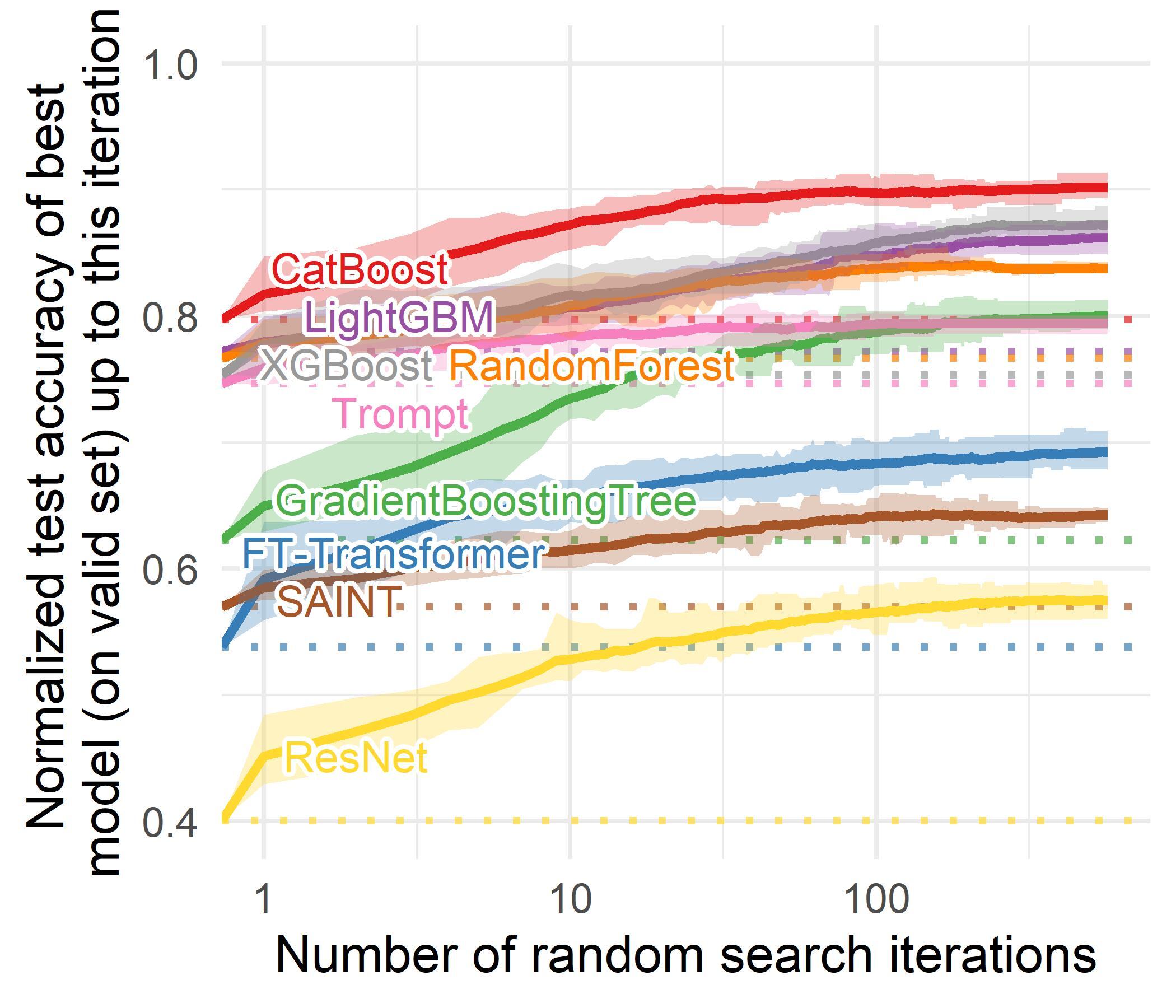
(a) Medium-sized classification task.

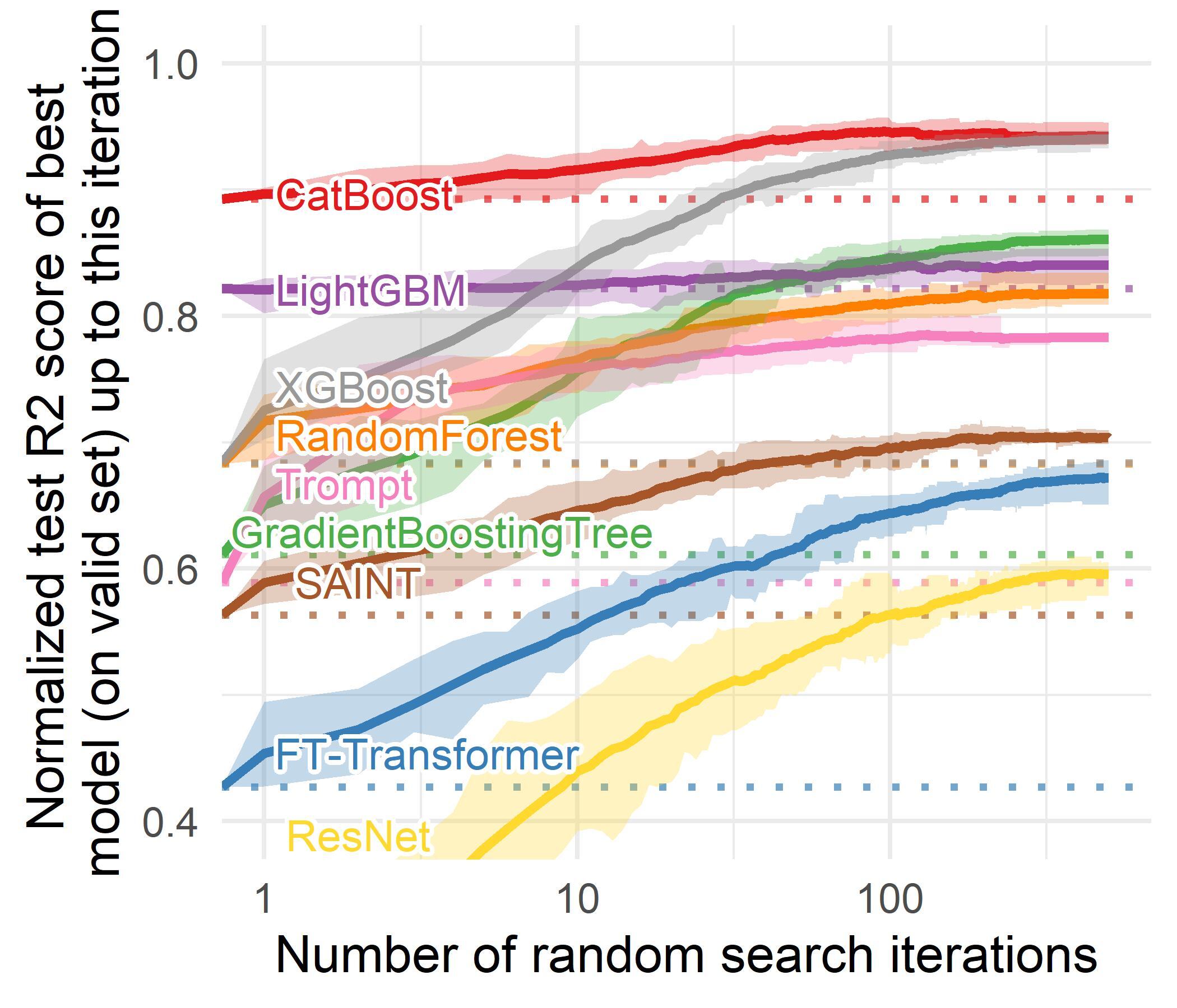
(b) Medium-sized regression task.

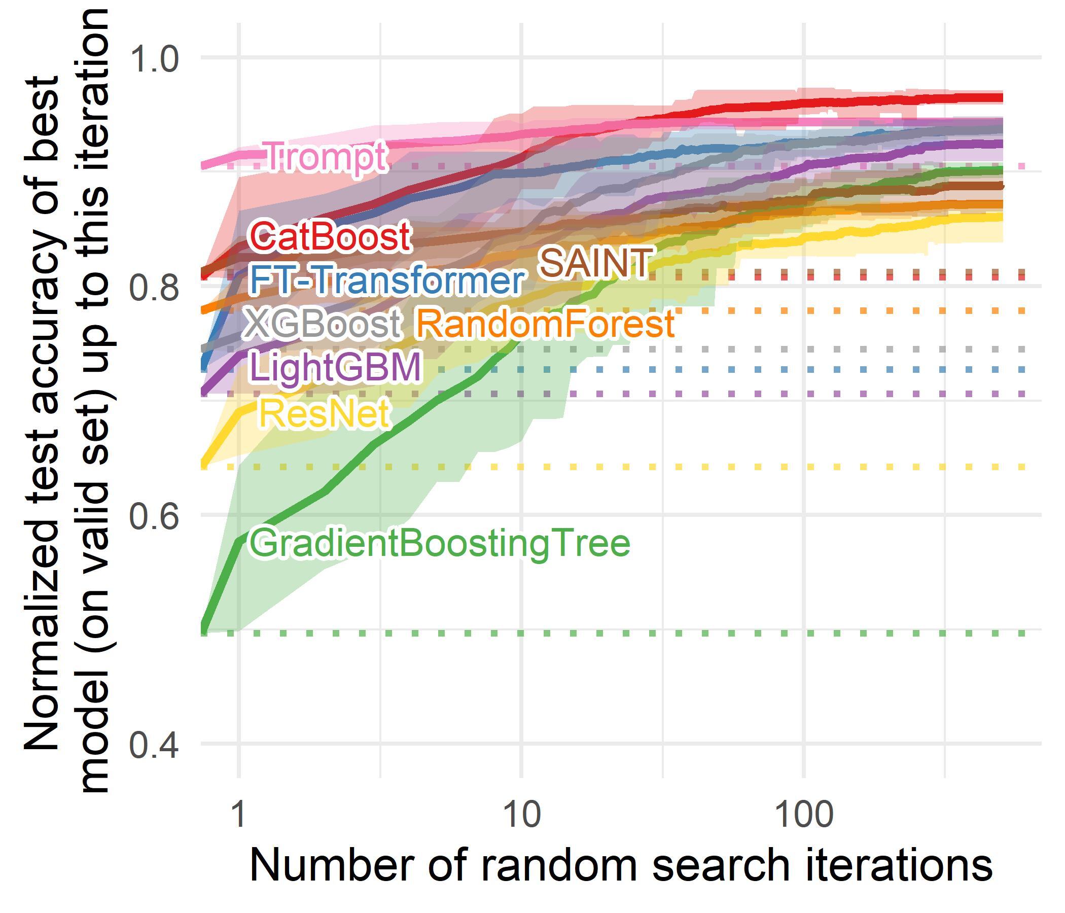
(c) Large-sized classification task.

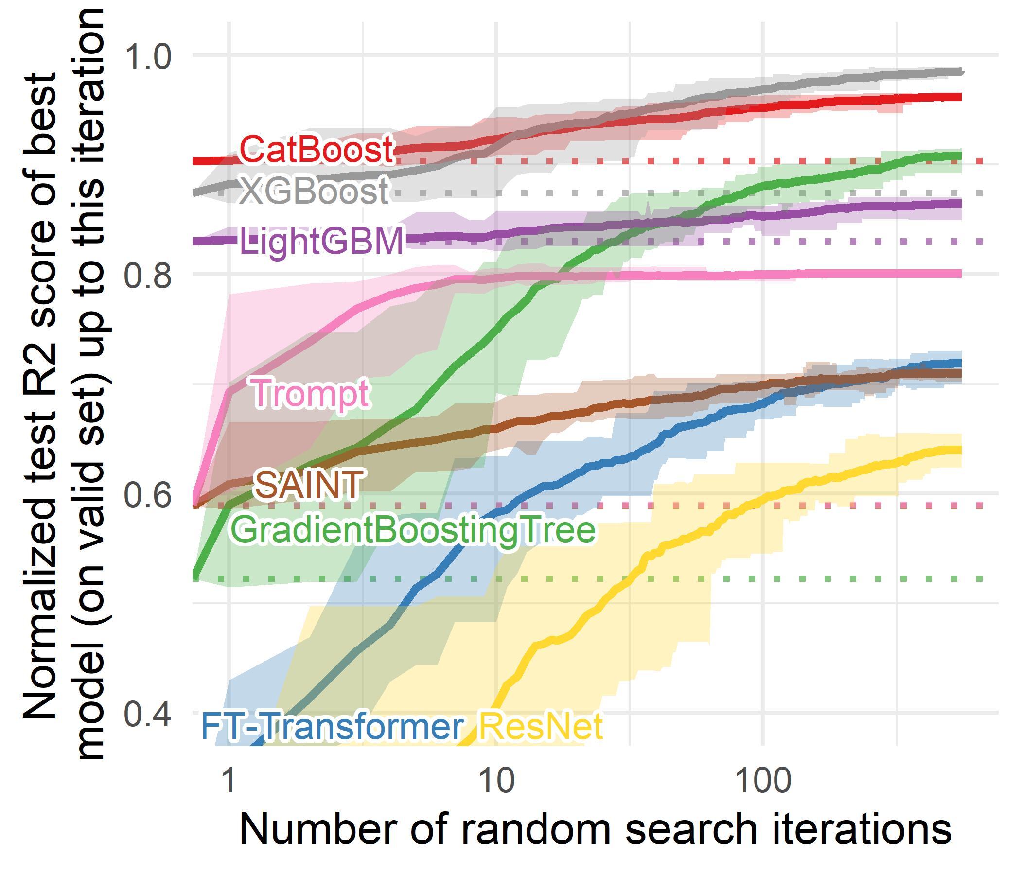
(d) Large-sized regression task.

Figure 1: Benchmark results.

1 Introduction

Tabular data plays a vital role in many real world applications, such as financial statements for banks to evaluate the credibility of a company, diagnostic reports for doctors to identify the aetiology of a patient, and customer records for e-commerce platforms to discover the potential interest of a customer. In general, tabular data can be used to record activities consisting of heterogeneous features and has many practical usages.

On the other hand, deep learning has achieved a great success in various domains, including computer vision, natural language processing (NLP) and robotics (He et al., 2016; Redmon et al., 2016; Gu et al., 2017; Devlin et al., 2018). Besides extraordinary performance, there are numerous benefits of the end-to-end optimization nature of deep learning, including (i) online learning with streaming data (Sahoo et al., 2017), (ii) multi-model integration that incorporates different types of input, e.g., image and text (Ramachandram & Taylor, 2017) and (iii) representation learning that realizes semi-supervised learning and generative modeling (Van Engelen & Hoos, 2020; Goodfellow et al., 2020).

Consequently, researchers have been dedicated to apply deep learning on tabular data, either through (i) transformer (Huang et al., 2020; Somepalli et al., 2021; Gorishniy et al., 2021) or (ii) inductive bias investigation (Katzir et al., 2020; Arik & Pfister, 2021).

Though many of the previous publications claimed that they have achieved the state of the art, further researches pointed that previous works were evaluated on favorable datasets and tree-based models still show superior performances in the realm of tabular data (Borisov et al., 2021; Gorishniy et al., 2021; Shwartz-Ziv & Armon, 2022). For a fair comparison between different algorithms, a standard benchmark for tabular data was proposed by (Grinsztajn et al., 2022). The benchmark, denoted as Grinsztajn45 in this work, consists of 45 curated datasets from various domains.

In this paper, we propose a novel prompt-inspired architecture, Trompt, which abbreviates Tabular Prompt. Prompt learning has played an important role in the recent development of language models. For example, GPT-3 can well handle a wide range of tasks with an appropriate prompt engineering (Radford et al., 2018; Brown et al., 2020). In Trompt, prompt is utilized to derive feature importances that vary in different samples. Trompt consists of multiple Trompt Cells and a shared Trompt Downstream as Figure 2. Each Trompt Cell is responsible for feature extraction, while the Trompt Downstream is for prediction.

The performance of Trompt is evaluated on the Grinsztajn45 benchmark and compared with three deep learning models and five tree-based models. Figure 1 illustrates the overall evaluation results on Grinsztajn45. The x-axis is the number of hyperparameter search iterations and y-axis is the normalized performance. In Figure 1, Trompt is consistently better than state-of-the-art deep learning models (SAINT and FT-Transformer) and the gap between deep learning models and tree-based models is narrowed.

Our key contributions are summarized as follows:

• The experiments are conducted on a recognized tabular benchmark, Grinsztajn45. Additionally, we add two well-performed tree-based models, LightGBM (Ke et al., 2017) and CatBoost (Prokhorenkova et al., 2018) to baselines.

• Trompt achieves state-of-the-art performance among deep learning models and narrows the performance gap between deep learning models and tree-based models.

• Thorough empirical studies and ablation tests were conducted to verify the design of Trompt. The results further shed light on future research directions of the architecture design of tabular neural network.

2 Related Work

In this section, we first discuss the prompt learning of language models. Secondly, we discuss two research branches of tabular neural networks, transformer and inductive bias investigation. Lastly, we discuss the differences between Trompt and the related works and highlight the uniqueness of our work.

2.1 Prompt Learning

The purpose of prompt learning is to transform the input and output of downstream tasks to the original task used to build a pre-trained model. Unlike fine-tuning that changes the task and usually involves updating model weights, a pre-train model with prompts can dedicate itself to one task. With prompt learning, a small amount of data or even zero-shot can achieve good results (Radford et al., 2018; Brown et al., 2020). The emergence of prompt learning substantially improves the application versatility of pre-trained models that are too large for common users to fine-tune.

To prompt a language model, one can insert a task-specific prompt before a sentence and hint the model to adjust its responses for different tasks (Brown et al., 2020). Prompts can either be discrete or soft. The former are composed of discrete tokens from the vocabulary of natural languages (Radford et al., 2018; Brown et al., 2020), while the latter are learned representations (Li & Liang, 2021; Lester et al., 2021).

2.2 Tabular Neural Network

Transformer. Self-attention has revolutionized NLP since 2017 (Vaswani et al., 2017), and soon been adopted by other domains, such as computer vision, reinforcement learning and speech recognition (Dosovitskiy et al., 2020; Chen et al., 2021; Zhang et al., 2020). The intention of transformer blocks is to capture the relationships among features, which can be applied on tabular data as well.

TabTransformer (Huang et al., 2020) is the first transformer-based tabular neural network. However, TabTransformer only fed categorical features to transformer blocks and ignored the potential relationships among categorical and numerical features. FT-Transformer (Gorishniy et al., 2021) fixed this issue through feeding both categorical and numerical features to transformer blocks. SAINT (Somepalli et al., 2021) further improved FT-Transformer through applying attentions on not only the feature dimensions but also the sample dimensions.

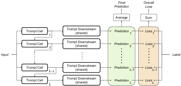
Figure 2: Overall architecture of the proposed Trompt.

Inductive Bias Investigation. Deep neural networks perform well on tasks with clear inductive bias. For example, Convolutional Neural Network (CNN) works well on images. The kernel of CNN is designed to capture local patterns since neighboring pixels usually relate to each other (LeCun et al., 1995). Recurrent Neural Networks (RNN) is widely used in language understanding because the causal relationship among words is well encapsulated through recurrent units (Rumelhart et al., 1986). However, unlike other popular tasks, the inductive bias of tabular data has not been well discovered.

Given the fact that tree-based model has been the solid state of the art for tabular data (Borisov et al., 2021; Gorishniy et al., 2021; Shwartz-Ziv & Armon, 2022), Net-DNF (Katzir et al., 2020) and TabNet (Arik & Pfister, 2021) hypothesized that the inductive bias for tabular data might be the learning strategy of tree-based model. The strategy is to find the optimal root-to-leaf decision paths by selecting a portion of the features and deriving the optimal split from the selected features in non-leaf nodes. To emulate the learning strategy, TabNet utilized sequential attention and sparsity regularization. On the other hand, Net-DNF theoretically proved that decision tree is equivalent to some disjunctive normal form (DNF) and proposed disjunctive neural normal form to emulate a DNF formula.

2.3 The Uniqueness of Trompt

We argue that the column importances of tabular data are not invariant for all samples and can be grouped into multiple modalities. Since prompt learning is born to adapt a model to multiple tasks, the concept is used in Trompt to handle multiple modalities. To this end, Trompt separates the learning strategy of tabular data into two parts. The first part, analogous to pre-trained models, focus on learning the intrinsic column information of a table. The second part, analogous to prompts, focus on diversifying the feature importances of different samples.

As far as our understanding, Trompt is the first prompt-inspired tabular neural network. Compared to transformer-based models, Trompt learns separated column importances instead of focusing on the interactions among columns. Compared to TabNet and Net-DNF, Trompt handle multiple modalities by emulating prompt learning instead of the branch split of decision tree.

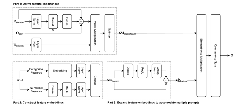
Figure 3: Architecture of a Trompt Cell.

3 Trompt

In this section, we elaborate on the architecture design of Trompt. As Figure 2 shows, Trompt consists of multiple Trompt Cells and a shared Trompt Downstream. Each Trompt Cell is responsible for feature extraction and providing diverse representations, while the Trompt Downstream is for prediction. The details of Trompt Cell and Trompt Downstream are discussed in Section 3.1 and Section 3.2, respectively. In Section 3.3, we further discuss the prompt learning of Trompt.

3.1 Trompt Cell

Figure 3 illustrates the architecture of a Trompt Cell, which can be divided into three parts. The first part derives feature importances ($\mathbf{M}_{\text{importance}}$) based on column embeddings ($\mathbf{E}_{\text{column}}$), the previous cell’s output ($\mathbf{O}_{\text{prev}}$) and prompt embeddings ($\mathbf{E}_{\text{prompt}}$). The second part transforms the input into feature embeddings ($\mathbf{E}_{\text{feature}}$) with two paths for categorical and numerical columns, respectively. The third part expands $\mathbf{E}_{\text{feature}}$ for the later multiplication.

The details of the first part are illustrated in Section 3.1.1 and the details of the second and third parts are illustrated in Section 3.1.2. Lastly, the generation of the output of a Trompt Cell is illustrated in Section 3.1.3.

3.1.1 Derive Feature Importances

Let $\mathbf{E}_{\text{column}}\in\mathbb{R}^{C\times{d}}$ be column embeddings and $\mathbf{E}_{\text{prompt}}\in\mathbb{R}^{P\times{d}}$ be prompt embeddings. $C$ is the number of columns of a table defined by the dataset, while $P$ and $d$ are hyperparameters for the number of prompts and the hidden dimension, respectively. Both $\mathbf{E}_{\text{column}}$ and $\mathbf{E}_{\text{prompt}}$ are input independent and trainable. Let $\mathbf{O}_{\text{prev}}\in\mathbb{R}^{B\times{P}\times{d}}$ be the previous cell’s output and $B$ be the batch size.

$\mathbf{O}_{\text{prev}}$ is fused with the prompt embeddings as Equations 1 and 2. Since $\mathbf{E}_{\text{prompt}}$ is input independent and lack a batch dimension, $\mathbf{E}_{\text{prompt}}$ is expanded to $\mathbf{SE}_{\text{prompt}}$ through the stack operation as Equation 1. Later, we concatenate $\mathbf{SE}_{\text{prompt}}$ and $\mathbf{O}_{\text{prev}}$ and then reduce the dimension of the concatenated tensor back to $\mathbb{R}^{B\times{P}\times{d}}$ for the final addition as Equation 2.

For the same reason as $\mathbf{E}_{\text{prompt}}$, the $\mathbf{E}_{\text{column}}$ is expanded to $\mathbf{SE}_{\text{column}}$ as Equation 3. Subsequently, feature importances are derived through Equation 4, where $\otimes$ is the batch matrix multiplication, $\intercal$ is the batch transpose, and the $\mathtt{softmax}$ is applied to the column axis.

$$\mathbf{SE}_{\text{prompt}}=\mathtt{stack}(\mathbf{E}_{\text{prompt}})\in\mathbb{R}^{B\times{P}\times{d}}$$ (1)

$$\begin{split}\mathbf{\hat{SE}}_{\text{prompt}}=&\mathtt{dense}(\mathtt{concat}(\mathbf{SE}_{\text{prompt}},\mathbf{O}_{\text{prev}}))\\ &+\mathbf{SE}_{\text{prompt}}\\ &+\mathbf{O}_{\text{prev}}\\ &\in\mathbb{R}^{B\times{P}\times{d}}\end{split}$$ (2)

$$\mathbf{SE}_{\text{column}}=\mathtt{stack}(\mathbf{E}_{\text{column}})\in\mathbb{R}^{B\times{C}\times{d}}$$ (3)

$$\mathbf{M}_{\text{importance}}=\mathtt{softmax}(\mathbf{\hat{SE}}_{\text{prompt}}\otimes\mathbf{SE}_{\text{column}}^{\intercal})\in\mathbb{R}^{B\times{P}\times{C}}$$ (4)

The output of the first part is $\mathbf{M}_{\text{importance}}\in\mathbb{R}^{B\times{P}\times{C}}$, which accommodates the feature importances yielded by $P$ prompts. Notice that the column embeddings are not connected to the input and the prompt embeddings are fused with the previous cell’s output. In Section 3.3, we further discuss these designs and their connections to the prompt learning of NLP.

3.1.2 Construct and Expand Feature Embeddings

In Trompt, categorical features are embedded through a embedding layer and numerical features are embedded through a dense layer as previous works (Somepalli et al., 2021; Gorishniy et al., 2021). The embedding construction procedure is illustrated in part two of Figure 3, where $\mathbf{E}_{\text{feature}}\in\mathbb{R}^{B\times{C}\times{d}}$ is the feature embeddings of the batch.

The shapes of $\mathbf{M}_{\text{importance}}$ and $\mathbf{E}_{\text{feature}}$ are $\mathbb{R}^{B\times{P}\times{C}}$ and $\mathbb{R}^{B\times{C}\times{d}}$, respectively. Since $\mathbf{E}_{\text{feature}}$ lacks the prompt dimension, Trompt expands $\mathbf{E}_{\text{feature}}$ into $\mathbf{\hat{E}}_{\text{feature}}\in\mathbb{R}^{B\times{P}\times{C}\times{d}}$ to accommodate the $P$ prompts by a dense layer in part three of Figure 3.

3.1.3 Generate Output

The output of Trompt Cell is the column-wise sum of the element-wise multiplication of $\mathbf{\hat{E}}_{\text{feature}}$ and $\mathbf{M}_{\text{importance}}$ as Equation 5, where $\odot$ is element-wise multiplication. Notice that, during element-wise multiplication, the shape of $\mathbf{M}_{\text{importance}}$ is considered $\mathbb{R}^{B\times{P}\times{C}\times{1}}$. In addition, since column is the third axis, the shape is reduced from $\mathbb{R}^{B\times{P}\times{C}\times{d}}$ to $\mathbb{R}^{B\times{P}\times{d}}$ after column-wise summation.

$$\mathbf{O}=\sum_{i=1}^{C}({\mathbf{\hat{E}}_{\text{feature}}\odot\mathbf{M}_{\text{importance}})_{:,:,i,:}}\in\mathbb{R}^{B\times{P}\times{d}}$$ (5)

Figure 4: Architecture of a Trompt Downstream.

3.2 Trompt Downstream

A Trompt Downstream makes a prediction based on a Trompt Cell’s output, which contains representations corresponding to $P$ prompt embeddings. To aggregate these representations, the weight for each prompt is first derived through a dense layer and a softmax activation function as Equation 6. Afterwards, the weighted sum is calculated as Equation 7.

The prediction is subsequently made through two dense layers as Equation 8, where $T$ is the target dimension. For classification tasks, $T$ is the number of target classes. For regression tasks, $T$ is set to 1. As Figure 2 shows, a sample gets a prediction through a Trompt Cell and thus multiple predictions through all cells. During training, the loss of each prediction is separately calculated and the loss is summed up to update model weights. During inference, on the other hand, predictions through all cells are simply averaged as the final prediction as Equation 9, where $L$ is the number of Trompt Cells.

$$\mathbf{W}_{\mathtt{prompt}}=\mathtt{softmax}(\mathtt{dense}(\mathbf{O}))\in\mathbb{R}^{B\times{P}}$$ (6)

$$\mathbf{\hat{O}}=\sum_{i=1}^{P}(\mathbf{W}_{\text{prompt}}\odot\mathbf{O})_{:,i,:}\in\mathbb{R}^{B\times{d}}$$ (7)

$$\mathbf{P}=\mathtt{dense}(\mathtt{relu}(\mathtt{dense}(\mathbf{\hat{O}})))\in\mathbb{R}^{B\times{T}}$$ (8)

$$\begin{split}&loss=\sum_{i=1}^{L}{\mathtt{loss\char 95\relax fn}(\mathbf{P}_{i}},y)\\ &pred=\sum_{i=1}^{L}{\mathbf{P}_{i}}/L\end{split}$$ (9)

Table 1: Analogy of the prompt learning of Trompt to that of NLP.

Problem Identification	Implemented by	Inspired by
Sample-invariant Intrinsic Properties	$\mathbf{E}_{\text{column}}$	Fixed Large Language Model
Sample-specific Feature Importances	$\mathbf{M}_{\text{importance}}$	Task-specific Predictions

3.3 Prompt Learning of Trompt

Trompt’s architecture is specifically designed for tabular data, taking into account the unique characteristics of this type of data and the impressive performance of tree-based models. Unlike conventional operations, the design may appear unconventional and detached from tabular data features. In this section, we explain the rationale behind Trompt’s network design and how we adapted prompt learning to a tabular neural network.

Tabular data is structured, with each column representing a specific dataset property that remains constant across individual samples. The success of tree-based models relies on assigning feature importances to individual samples. This concept has been explored in models such as TabNet (Arik & Pfister, 2021) and Net-DNF (Katzir et al., 2020). However, tree-based algorithms do not explicitly assign feature importances to individual samples. Instead, importances vary implicitly along the path from the root to a leaf node. Only the columns involved in this path are considered important features for the samples reaching the corresponding leaf node, representing sample-specific feature importances.

Given the fundamental characteristic of tabular data and the learning strategy of tree-based models, Trompt aims to combine the intrinsic properties of columns with sample-specific feature importances using a prompt learning-inspired architecture from NLP (Radford et al., 2018; Brown et al., 2020). Trompt employs column embeddings to represent the intrinsic properties of each column and prompt embeddings to prompt column embeddings, generating feature importances for given prompts. Both column embeddings and prompt embeddings are invariant across samples. However, before prompting column embeddings with prompt embeddings, the prompt embeddings are fused with the output of the previous Trompt Cell as shown in Equation 2, enabling input-related representations to flow through and derive sample-specific feature importances. The ”prompt” mechanism in Trompt is implemented as a matrix multiplication in Equation 4.

A conceptual analogy of Trompt’s prompt learning approach to NLP is presented in Table 1. It’s important to note that the implementation details of prompt learning differ substantially between tabular data and NLP tasks due to the fundamental differences between the two domains. Therefore, appropriate adjustments must be made to bridge these two domains.

4 Experiments

In this section, the experimental results and analyses are presented. First, we elaborate on the settings of experiments and the configurations of Trompt in Section 4.1. Second, the performance of Trompt on Grinsztajn45 is reported in Section 4.2. Third, ablation studies regarding the hyperparameters and the architecture of Trompt are studied in Section 4.3. Lastly, the interpretability of Trompt is investigated using synthetic and real-world datasets in Section 4.4.

4.1 Setup

The performance and ablation study of Trompt primarily focus on the Grinsztajn45 benchmark (Grinsztajn et al., 2022) . This benchmark comprises datasets from various domains and follows a unified methodology for evaluating different models, providing a fair and comprehensive assessment. Furthermore, we evaluate the performance of Trompt on datasets selected by FT-Transformer and SAINT to compare it with state-of-the-art tabular neural networks.

For interpretability analysis, we follow the experimental settings of TabNet (Arik & Pfister, 2021). This involves using two synthetic datasets (Syn2 and Syn4) and a real-world dataset (mushroom) to visualize attention masks.

The settings of Grinsztajn45 are presented in Section 4.1.1 and the implementation details of Trompt are presented in Section 4.1.2. Furthermore, the settings of datasets chosen by FT-Transformer and SAINT are provided in Section B.2 and Section B.3, respectively.

4.1.1 Settings of Grinsztajn45

To fairly evaluate the performance, we follow the configurations of Grinsztajn45, including train test data split, data preprocessing and evaluation metric. Grinsztajn45 comprises two kinds of tasks, classification tasks and regression tasks. Please see Section A.1 and Section A.2 for the dataset selection criteria and dataset normalization process of Grinsztajn45. The tasks are further grouped according to (i) the size of datasets (medium-sized and large-sized) and (ii) the inclusion of categorical features (numerical only and heterogeneous).

In addition, we make the following adjustments: (i) models with incomplete experimental results in (Grinsztajn et al., 2022) are omitted, (ii) two well-performed tree-based models are added for comparison, and (iii) Trompt used a hyperparameter search space smaller than its opponents. The details of the adjustments are described in Section A.3 and Section A.4.

4.1.2 Implementation Details

Trompt is implemented using PyTorch. The default hyperparameters are shown in Table 2. The size of embeddings and the hidden dimension of dense layers are configured $d$. Note that only the size of column and prompt embeddings must be the same by the architecture design. The hidden dimension of dense layers is set as $d$ to reduce hyperparameters and save computing resources. On the other hand, the number of prompts and the number of Trompt Cells are set to $P$ and $L$. Please refer to Appendix F for the hyperparameter search spaces for all baselines and Trompt.

Table 2: Default hyperparameters of Trompt.

Hyperparameter	Symbol	Value
Feature Embeddings Prompt/Column Embeddings Hidden Dimension	$d$	128
Prompts	$P$	128
Layer	$L$	6

4.2 Evaluation Results

The results of classification tasks are discussed in Section 4.2.1 and the results of regression tasks are discussed in Section 4.2.2. The evaluation metrics are accuracy and r2-score for classification and regression tasks, respectively. In this section, we report an overall result and leave results of individual datasets in Section B.1. In addition, the evaluation results on datasets chosen by FT-Transformer and SAINT are provided in Section B.2 and Section B.3, respectively.

4.2.1 Classification

On the medium-sized classification tasks, Figure 5 shows that Trompt outperforms DNN models. The curve of Trompt is consistently above deep neural networks (SAINT, FT-Transformer and ResNet) on tasks with and without categorical features. Additionally, Trompt narrows the gap between deep neural networks and tree-based models, especially on the tasks with heterogeneous features. In Figure 5(b), Trompt seems to be a member of the leading cluster with four tree-based models. The GradientBoostingTree starts slow but catches up the leading cluster in the end of search. The other deep neural networks forms the second cluster and have a gap to the leading one.

On the large-sized classification tasks, tree-based models remain the leading positions but the gap to deep neural networks is obscure. This echoes that deep neural networks requires more samples for training (LeCun et al., 2015). Figure 6(a) shows that Trompt outperforms ALL models on the task with numerical features and Figure 6(b) shows that Trompt achieves a comparable performance to FT-Transformer on tasks with heterogeneous features.

With the small hyperparameter search space, the curve of Trompt is relatively flat. The flat curve also suggests that Trompt performs well with its default hyperparameters. Its performance after an exhausted search is worthy of future exploring.

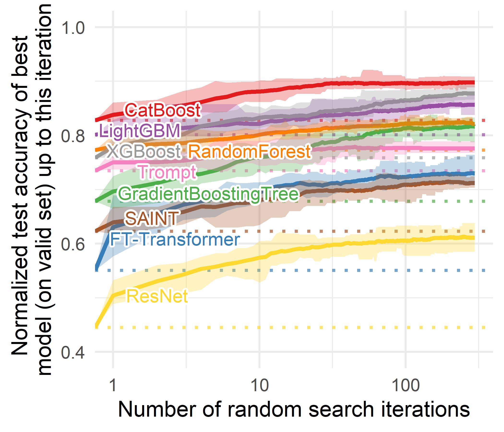
(a) Numerical features only.

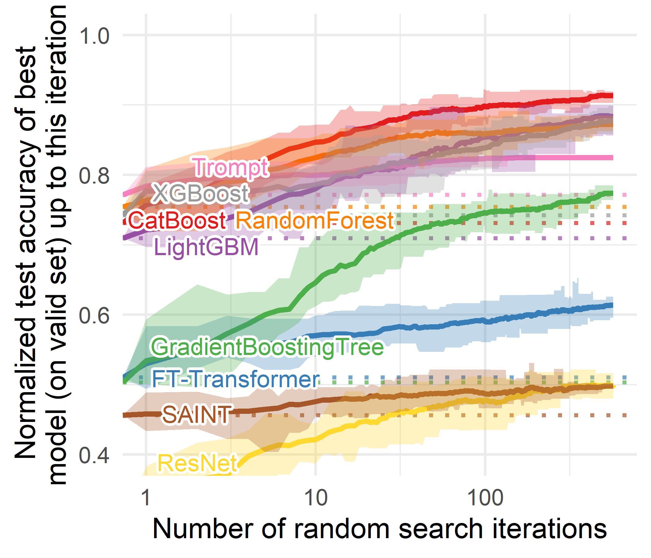
(b) Heterogeneous features.

Figure 5: Benchmark on medium-sized classification datasets.

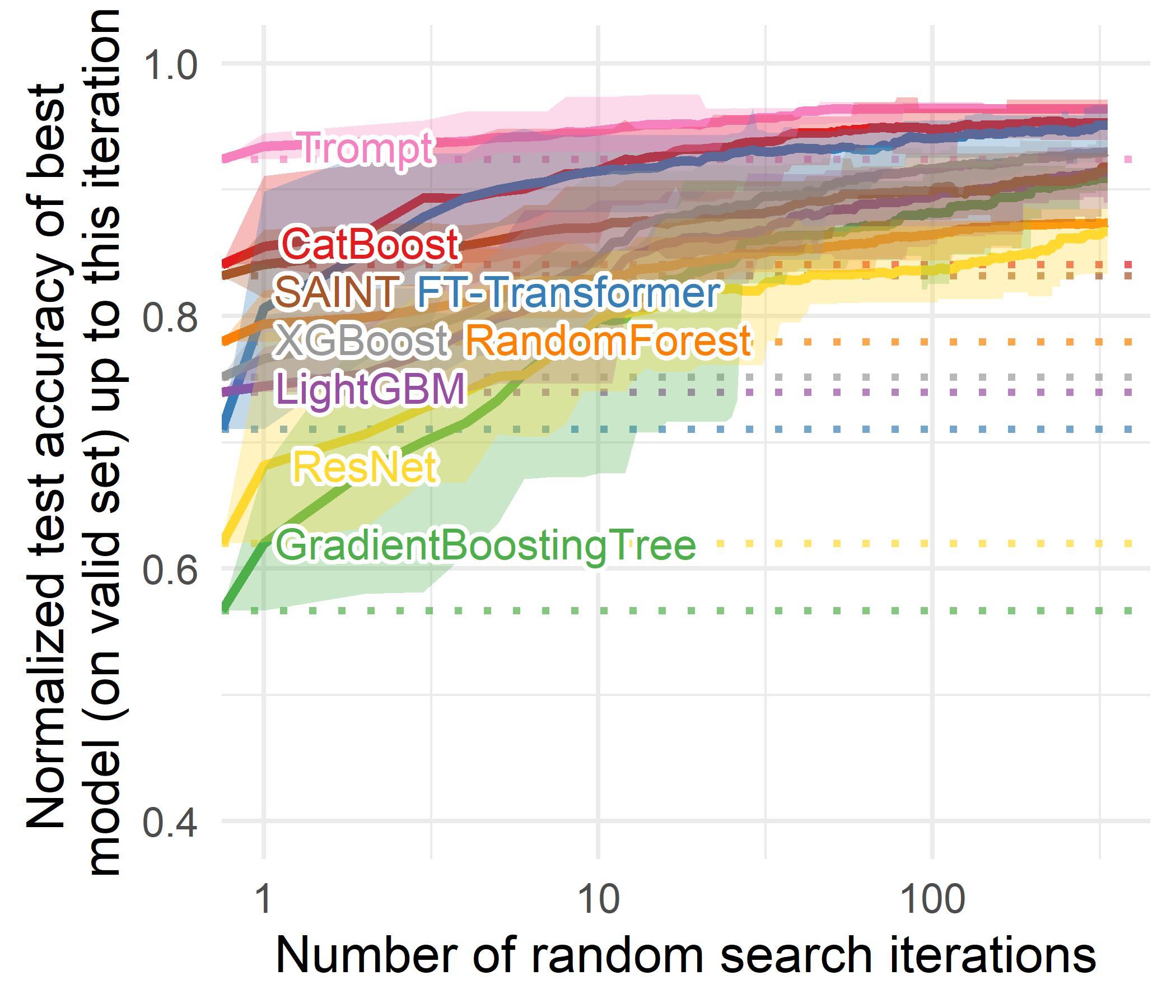
(a) Numerical features only.

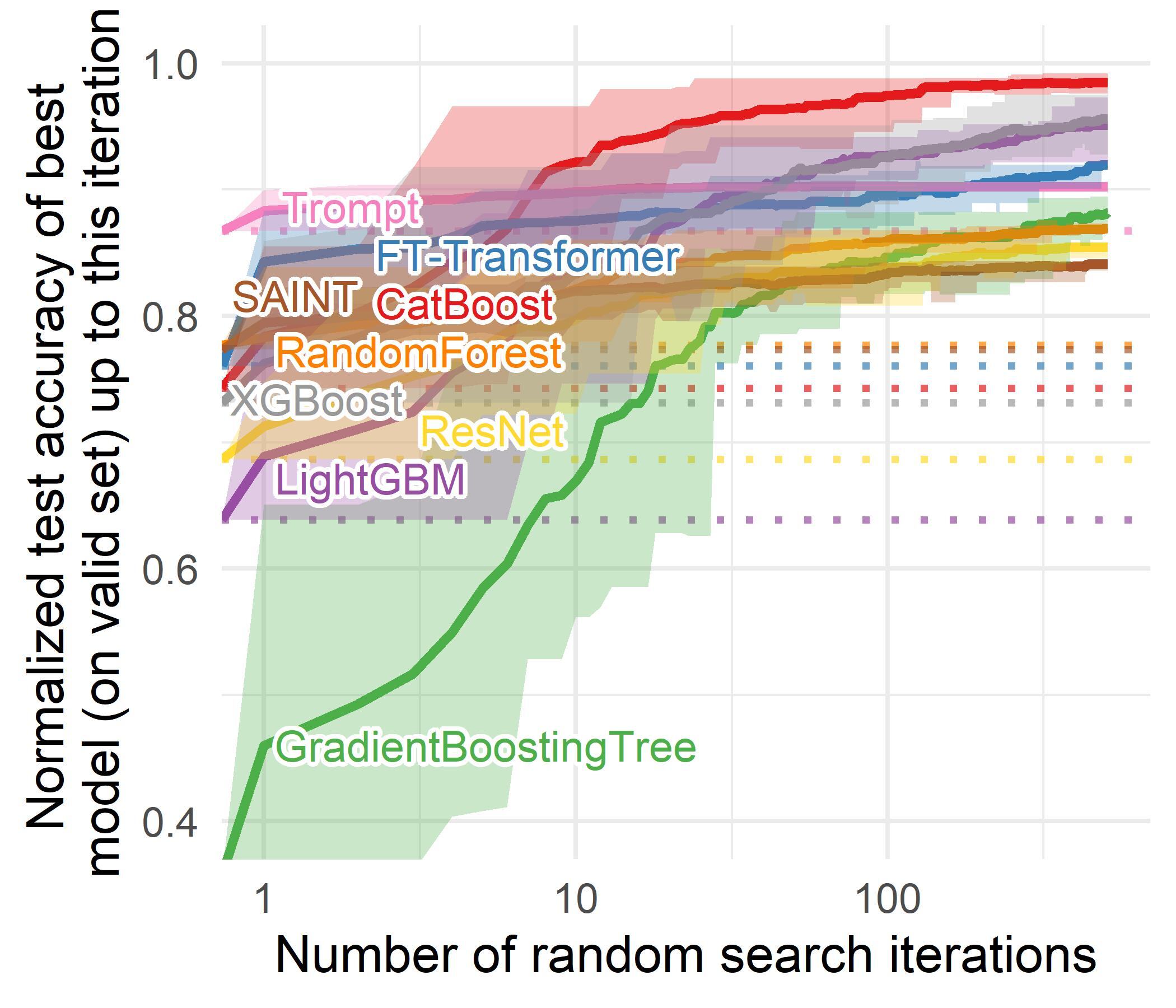
(b) Heterogeneous features.

Figure 6: Benchmark on large-sized classification datasets.

4.2.2 Regression

On the medium-sized regression tasks, Figure 7 shows that Trompt outperforms deep neural networks as the curves of Trompt are consistently higher than SAINT, FT-Transformer and ResNet on tasks with and without categorical features. The gap between deep neural networks and tree-based models is less obvious in Figure 7(a) than that in Figure 7(b). On the tasks with numerical features only, Trompt achieves a comparable performance with random forest. On the tasks with heterogeneous features, Trompt narrows the gap but is below all the tree-based models.

On the large-sized regression tasks with numerical features only, Figure 8(a) shows that Trompt is slightly worse than SAINT and FT-Transformer in the end of search. On the large-sized regression tasks with heterogeneous features, Figure 8(b) shows that Trompt outperforms deep neural networks with a large margin.

In general, deep learning models are not good at handling categorical features. Trompt alleviates this weakness as shown in all tasks with heterogeneous features in Figure 5–Figure 8. Trompt achieves superior performance over state-of-the-art deep neural networks except on the large-sized regression tasks with numerical features only.

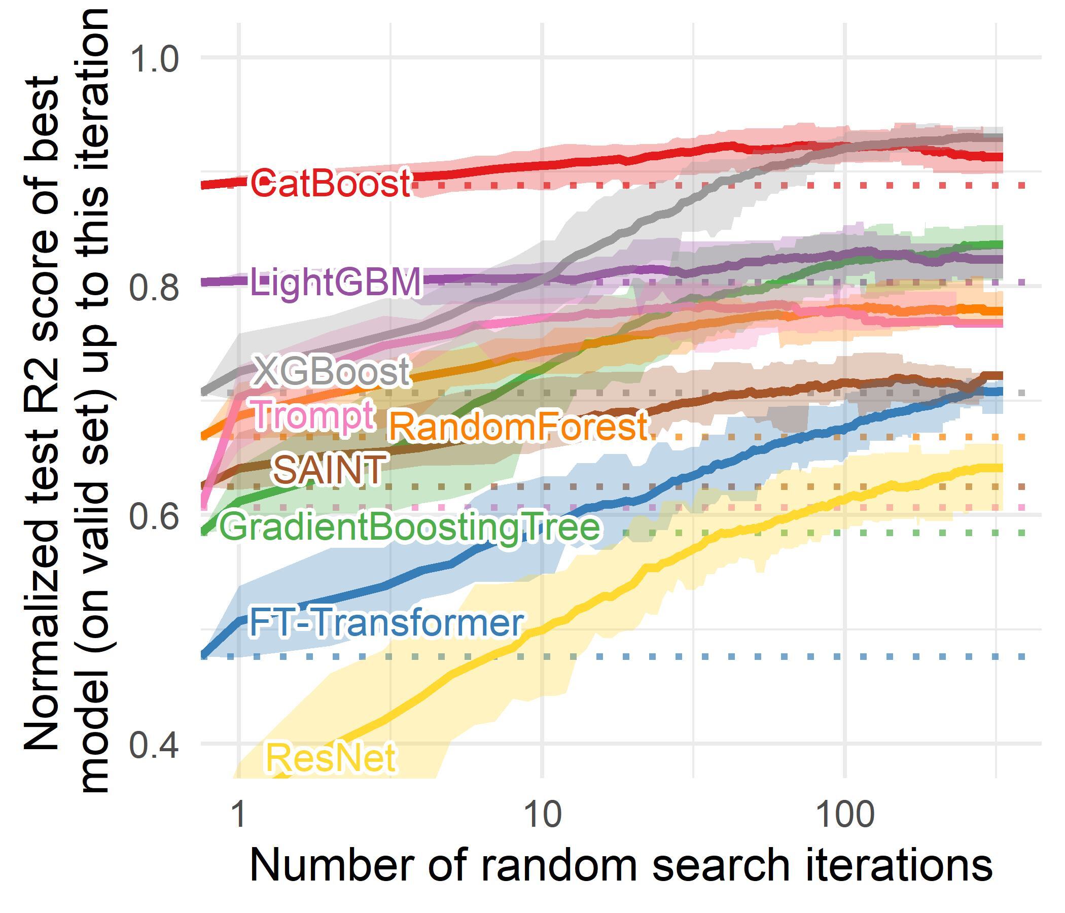
(a) Numerical features only.

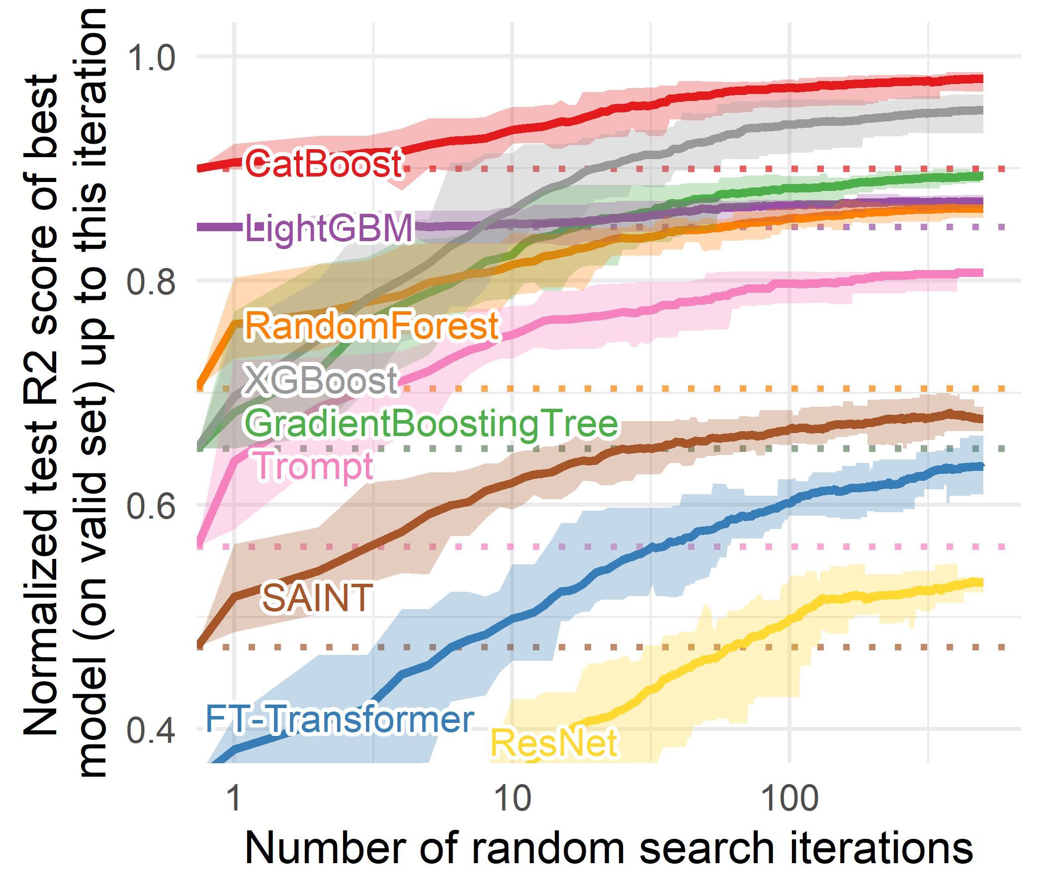
(b) Heterogeneous features.

Figure 7: Benchmark on medium-sized regression datasets.

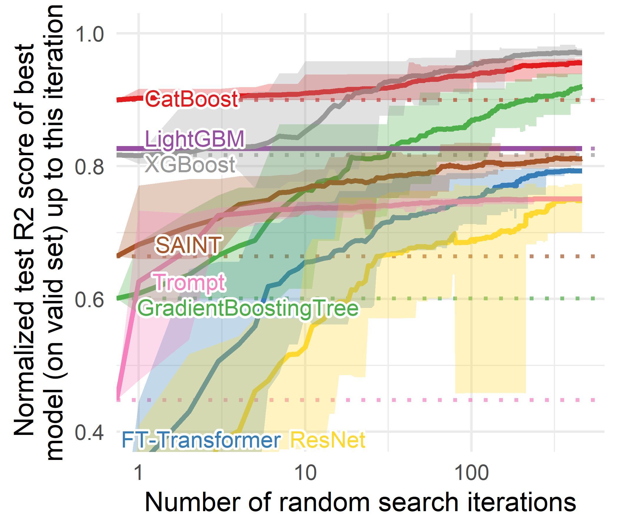
(a) Numerical features only.

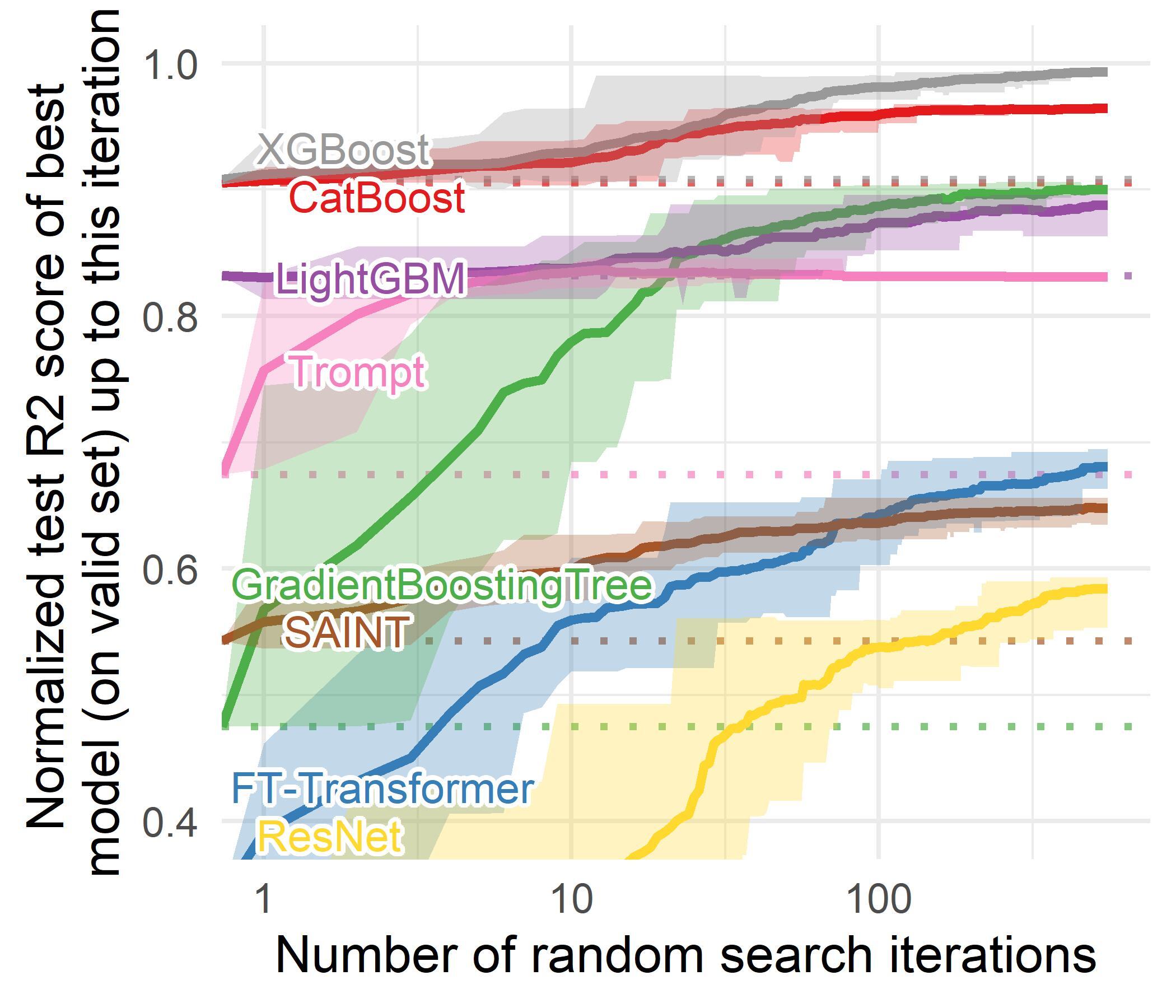
(b) Heterogeneous features.

Figure 8: Benchmark on large-sized regression datasets.

4.3 Ablation Study

In this subsection, we discuss the ablation study results of Trompt regarding hyperparameters and architecture design. Please refer to Appendix C for the settings of the ablation study. In the main article, we report two major ablations on (i) the number of prompts and (ii) the necessity of expanding feature embeddings by a dense layer. Other ablations can be found in Appendix D.

Ablations on the number of prompts. Prompt embeddings ($\mathbf{E}_{\text{prompt}}$) stand a vital role to derive the feature importances. Here we discuss the effectiveness of adjusting the number of prompts.

As shown in Table 3, setting the number of prompts to one results in the worse results. However, halving and doubling the default number (128) do not have much effect on the performance. The results demonstrate that Trompt is not sensitive to the number of prompts, as long as the number of prompts is enough to accommodate the modalities of the dataset.

Table 3: The performance of different number of prompts.

	1	64	128 (default)	256
Classification	$79.74\%$	$81.76\%$	$81.81\%$	$81.85\%$
Regression	$72.07\%$	$74.11\%$	$74.15\%$	$74.14\%$

Ablations on expanding feature embeddings by a dense layer. Part three of Figure 3 uses a dense layer to expand feature embeddings to accommodate $P$ prompts. Here we discuss the necessity of the dense layer.

As you can see in Table 4, adding a dense layer really leads to better results and is a one of the key architecture designs of Trompt. By design, adding the dense layer enables Trompt to generate different feature embeddings for each prompt. Without the dense layer, Trompt is degraded to a simplified situation where each prompt uses the same feature embeddings. The results of Table 3 and Table 4 suggest that the variation of feature importances, which comes from both the prompt embedding and the expansion dense layer, is the key to the excellent performance of Trompt.

Table 4: The performance of with and without applying feature transformation on Input Transform.

	w (default)	w/o
Classification	$81.81\%$	$80.76\%$
Regression	$74.15\%$	$73.73\%$

Table 5: The top-3 importance score ratio on the mushroom dataset.

	1st	2nd	3rd
RandomForest	odor ($15.11\%$)	gill-size ($12.37\%$)	gill-color ($10.42\%$)
XGBoost	spore-print-color ($29.43\%$)	odor ($22.71\%$)	cap-color ($14.07\%$)
LightGBM	spore-print-color ($22.08\%$)	gill-color ($14.95\%$)	odor ($12.96\%$)
CatBoost	odor ($72.43\%$)	spore-print-color ($10.57\%$)	gill-size ($2.71\%$)
GradientBoostingTree	gill-color ($31.08\%$)	spore-print-color ($19.89\%$)	odor ($17.44\%$)
Trompt (ours)	odor ($24.93\%$)	gill-size ($8.13\%$)	gill-color ($5.73\%$)

4.4 Interpretability

Besides outstanding performance, tree-based models are well-known for their interpretability. Here we explore whether Trompt can also provide concise feature importances that highlighted salient features. To investigate this, we conduct experiments on both synthetic datasets and real-world datasets, following the experimental design of TabNet (Arik & Pfister, 2021). To derive the feature importances of Trompt for each sample, $\mathbf{M}_{\text{importance}}\in\mathbb{R}^{B\times{P}\times{C}}$ is reduced to $\mathbf{\hat{M}}_{\text{importance}}\in\mathbb{R}^{B\times{C}}$ as Equation 10, where the weight of $\mathbf{M}_{\text{importance}}$ is the $\mathbf{W}_{\text{prompt}}$ of Equation 6.

Notice that all Trompt Cells derive separated feature importances. We demonstrate the averaged results of all cells here and leave the results of each cell in Section E.1.

$$\mathbf{\hat{M}}_{\text{importance}}=\sum_{i=1}^{P}(\mathbf{W}_{\text{prompt}}\odot\mathbf{M}_{\text{importance}})_{:,i,:}\in\mathbb{R}^{B\times{C}}$$ (10)

Synthetic datasets. The Syn2 and Syn4 datasets are used to study the feature importances learned by each model (Chen et al., 2018). A model is trained on oversampled training set (10k to 100k) using default hyperparameters and evaluated on 20 randomly picked testing samples. The configuration is identical to that in TabNet (Arik & Pfister, 2021).

Figure 9 and Figure 10 compare the important features of the dataset and those learned by Trompt. In the Syn2 dataset, features 2–5 are important (Figure 9(a)) and Trompt excellently focuses on them (Figure 9(b)). In the Syn4 dataset, either features 0–1 or 2–5 could be important based on the value of feature 10 (Figure 10(a)). As Figure 10 shows, Trompt still properly focuses on features 0–5 and discovers the influence of feature 10.

(a) Important features.

(b) Feature importances of Trompt.

Figure 9: Attention mask on Syn2 dataset (synthetic).

(a) Important features.

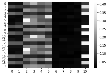
(b) Feature importances of Trompt.

Figure 10: Attention mask on Syn4 dataset (synthetic).

Real-world datasets. The mushroom dataset (Dua & Graff, 2017) is used as the real-world dataset for visualization as TabNet (Arik & Pfister, 2021). With only the Odor feature, most machine learning models can achieve $>95\%$ test accuracy (Arik & Pfister, 2021). As a result, a high feature importance is expected on Odor.

Table 5 shows the three most important features of Trompt and five tree-based models. As shown, all models place Odor in their top three. The second and third places of Trompt, gill-size and gill-color, also appear in the top three of the other models. Actually, cap-color is selected only by XGBoost. If it is excluded, the union of the top important features of all models comes down to four features. The one Trompt missed is spore-print-color, which is the fifth place of Trompt. Overall speaking, the important features selected by Trompt are consistent with those by tree-based models, and can therefore be used in various analyses that are familiar in the field of machine learning.

To further demonstrate that the experimental results were not ad-hoc, we repeat the experiments on additional real-world datasets. Please see Section E.2 for the details and experimental results.

5 Discussion

In this section, we further explore the “prompt” mechanism of Trompt. Section 5.1 clarifies the underlying hypothesis of how the prompt learning of Trompt fits for tabular data. In addition, as Trompt is partially inspired by the learning strategy of tree-based models, we further discussed the difference between Trompt and tree-based models in Section 5.2.

5.1 Further exploration of the ”prompt” mechanism in Trompt

The ”prompt” mechanism in Trompt is realized as Equation 4. This equation involves a matrix multiplication of expanded prompt embeddings ($\mathbf{\hat{SE}}_{\text{prompt}}\in\mathbb{R}^{B\times{P}\times{d}}$) and the transpose of expanded column embeddings ($\mathbf{SE}_{\text{column}}\in\mathbb{R}^{B\times{C}\times{d}}$). It results in $\mathbf{M}_{\text{importance}}\in\mathbb{R}^{P\times{C}}$, which represents prompt-to-column feature importances. The matrix multiplication calculates the cosine-based distance between $\mathbf{\hat{SE}}_{\text{prompt}}$ and $\mathbf{SE}_{\text{column}}$, and favors high similarity between the sample-specific representations and sample-invariant intrinsic properties.

To make it clearer, $\mathbf{\hat{SE}}_{\text{prompt}}$ consists of $P$ embeddings that are specific to individual samples, except for the first Trompt Cell where $\mathbf{O}_{\text{prev}}$ is a zero tensor since there is no previous Trompt Cell, as stated in Equations 1 and 2. On the other hand, $\mathbf{SE}_{\text{column}}$ consists of $C$ embeddings that represent intrinsic properties specific to a tabular dataset as stated in Equation 3.

Unlike self-attention, which calculates the distance between queries and keys and derives token-to-token similarity measures, Trompt calculates the distance between $\mathbf{\hat{SE}}_{\text{prompt}}$ and $\mathbf{SE}_{\text{column}}$ in LABEL:{eq:soft-select} to derive sample-to-intrinsic-property similarity measures. The underlying idea of the calculation is to capture the distance between each sample and intrinsic property of a tabular dataset and we hypothesize that incorporating the intrinsic properties into the modeling of a tabular neural network might help making good predictions.

5.2 The differences between Trompt and Tree-based Models

As discussed in Section 3.3, the idea of using prompt learning to derive feature importances, is inspired by the learning algorithm of tree-based models and the intrinsic properties of tabular data. As a result, Trompt and tree-based models share a common characteristic in that they enable sample-dependent feature importances. However, there are two main differences between them. First, to incorporate the intrinsic properties of tabular data, Trompt uses column embeddings to share the column information across samples, while the learning strategy of tree-based models learn column information in their node-split nature. Second, Trompt and tree-based models use different techniques to learn feature importance. Trompt derives feature importances explicitly through prompt learning, while tree-based models vary the feature importances implicitly in the root-to-leaf path.

6 Conclusion

In this study, we introduce Trompt, a novel network architecture for tabular data analysis. Trompt utilizes prompt learning to determine varying feature importances in individual samples. Our evaluation shows that Trompt outperforms state-of-the-art deep neural networks (SAINT and FT-Transformer) and closes the performance gap between deep neural networks and tree-based models.

The emergence of prompt learning in deep learning is promising. While the design of Trompt may not be intuitive or perfect for language model prompts, it demonstrates the potential of leveraging prompts in tabular data analysis. This work introduces a new strategy for deep neural networks to challenge tree-based models and future research in this direction can explore more prompt-inspired architectures.

Appendix A Settings of Grinsztajn45

In this section, we provide brief summaries with regard to dataset selection criteria in Section A.1, dataset normalization in Section A.2, baseline models in Section A.3 and hyperparameter search mechanism in Section A.4.

A.1 Dataset Selection Criteria

Grinsztajn45 (Grinsztajn et al., 2022) selects 45 tabular datasets from various domains mainly provided by OpenML (Vanschoren et al., 2013), which is listed in section A.1 of their paper.

The dataset selection criteria are summarized below. Please refer to section 3.1 of the original paper for detailed selection criteria.

• The datasets contain heterogeneous features.

• They are not high dimensional.

• They contain I.I.D. data.

• They contain real-world data.

• They are not too small.

• They are not too easy.

• They are not deterministic.

A.2 Dataset Normalization

To ensure the homogeneity of the datasets and focus on challenges specific to tabular data, Grinsztajn45 did some modifications to the datasets to make sure that the datasets in the benchmark conform to the following criteria. Please refer to section 3.2 of the original paper for detailed modification.

• The training sets are truncated to medium-sized (10,000) or large-sized (50,000).

• All missing data were removed from the datasets.

• The classes are balanced.

• Categorical features with more than 20 items were removed

• Numerical features with less than 10 unique values were removed.

• Numerical features with 2 unique values are converted to categorical features.

A.3 Baseline Models

The paper by Grinsztajn45 presents the performance of four DNN models and four tree-based models. The DNN models include MLP (Gorishniy et al., 2021), ResNet (Gorishniy et al., 2021), FT-Transformer (Gorishniy et al., 2021), and SAINT (Somepalli et al., 2021). The tree-based models consist of RandomForest (Breiman, 2001), GradientBoostingTree (Friedman, 2001), XGBoost (Chen et al., 2015), and HistGradientBoostingTree (scikit learn, 2023a).

However, two models, namely MLP (Gorishniy et al., 2021) and HistGradientBoostingTree (scikit learn, 2023a), were omitted from the evaluation due to incomplete experimental results in Grinsztajn45 (Grinsztajn et al., 2022). To provide a comprehensive comparison, we have included LightGBM (Ke et al., 2017) and CatBoost (Prokhorenkova et al., 2018) as additional models. These models were selected based on their excellent performance and popularity.

A.4 Hyperparameter Search Mechanism

Grinsztajn45 evaluates models based on the results of a random search that consumes 20,000 compute-hours, as mentioned in Section 3.3 of the paper (Grinsztajn et al., 2022). Since different models have varying inference and update times, the number of random search iterations completed within the same compute-hour differs for each model. For instance, Model A may perform around two hundred iterations, while Model B may perform around three hundred iterations within 20,000 hours. To ensure a fair evaluation, the iterations are truncated based on the minimum iteration count among all the compared models.

Due to limited computing resources, we have chosen a small search space (Table 30) consisting of 40 parameter combinations. To avoid unfairly truncating random search results of other models, and compromising the low search iterations of Trompt, we duplicated the grid search results of Trompt to exceed the lowest search iteration count among the models provided by Grinsztajn45. For instance, if the lowest search iteration of a model was three hundreds, the search results of Trompt will be oversampled to surpass three hundreds and avoid being the lower bound, so other models can retain same search iterations as provided by Grinsztajn45. As a result, the other models can retain the same search iterations as provided by Grinsztajn45.

Grinsztajn45’s suggested evaluation procedure involves an extensive hyperparameter search that explores hundreds of parameter combinations. However, due to limited computing resources, we have selected a smaller search space of 40 parameter combinations (Table 30 in Appendix F) for Trompt. Please refer to Appendix F for the hyperparameter search spaces of all models.

Appendix B More Evaluation Results

In Section B.1, we present additional evaluation results for Grinsztajn45, which expand upon the findings and analysis presented in the original paper (Grinsztajn et al., 2022). These additional results provide further insights and contribute to a more comprehensive understanding of the evaluated models.

Furthermore, we include evaluation results on different datasets using the datasets selected by FT-Transformer (Gorishniy et al., 2021) and SAINT (Somepalli et al., 2021) in Section B.2 and Section B.3, respectively. By applying these datasets to the models, we aim to assess the performance of Trompt in different scenarios and gain a deeper understanding of its capabilities and generalizability.

B.1 Grinsztajn45

In main paper, we have discussed the overall performance of Trompt using the learning curves during hyperparameter optimization. In this section, we present quantitative evaluation results of both default and optimized hyperparameters. In addition, we provide the figures of individual datasets for reference.

The quantitative evaluation results of classification and regression tasks are discussed in Section B.1.1 and Section B.1.2 respectively. For classification datasets, we use accuracy as the evaluation metric. For regression datasets, we use r2-score as the evaluation metric. As a result, in both categories, the higher the number, the better the result. Besides evaluation metrics, the ranking of each model is also provided. To derive ranking, we calculate the mean and standard deviation of all rankings on datasets of a task. Notice that since the names of some datasets are long, we first denote each dataset a notation in Tables 6, 7 and 8 and use them in following tables.

Table 6: Notation of medium-sized datasets (1).

Notation	Dataset
A1	KDDCup09_upselling
A2	compass
A3	covertype
A4	electricity
A5	eye_movements
A6	rl
A7	road-safety
B1	Higgs
B2	MagicTelescope
B3	MiniBooNE
B4	bank-marketing
B5	california
B6	covertype
B7	credit
B8	electricity
B9	eye_movements
B10	house_16H
B11	jannis
B12	kdd_ipums_la_97-small
B13	phoneme
B14	pol
B15	wine

Table 7: Notation of medium-sized datasets (2).

Notation	Dataset
C1	Bike_Sharing_Demand
C2	Brazilian_houses
C3	Mercedes_Benz_Greener_Manufacturing
C4	OnlineNewsPopularity
C5	SGEMM_GPU_kernel_performance
C6	analcatdata_supreme
C7	black_friday
C8	diamonds
C9	house_sales
C10	nyc-taxi-green-dec-2016
C11	particulate-matter-ukair-2017
C12	visualizing_soil
C13	yprop_4_1
D1	Ailerons
D2	Bike_Sharing_Demand
D3	Brazilian_houses
D4	MiamiHousing2016
D5	california
D6	cpu_act
D7	diamonds
D8	elevators
D9	fifa
D10	house_16H
D11	house_sales
D12	houses
D13	medical_charges
D14	nyc-taxi-green-dec-2016
D15	pol
D16	sulfur
D17	superconduct
D18	wine_quality
D19	year

Table 8: Notation of large-sized datasets.

Notation	Dataset
$\mathbb{A}$1	covertype
$\mathbb{A}$2	road-safety
$\mathbb{B}$1	covertype
$\mathbb{B}$2	Higgs
$\mathbb{B}$3	MiniBooNE
$\mathbb{B}$4	jannis
$\mathbb{C}$1	black_friday
$\mathbb{C}$2	diamonds
$\mathbb{C}$3	nyc-taxi-green-dec-2016
$\mathbb{C}$4	particulate-matter-ukair-2017
$\mathbb{C}$5	SGEMM_GPU_kernel_performance
$\mathbb{D}$1	diamonds
$\mathbb{D}$2	nyc-taxi-green-dec-2016
$\mathbb{D}$3	year

B.1.1 Classification

The evaluation results for medium-sized classification tasks are presented in Table 9 for heterogeneous features, and in Tables 10 and 11 for numerical features only.

For large-sized classification tasks, the results can be found in Table 12 for heterogeneous features, and in Table 13 for numerical features only.

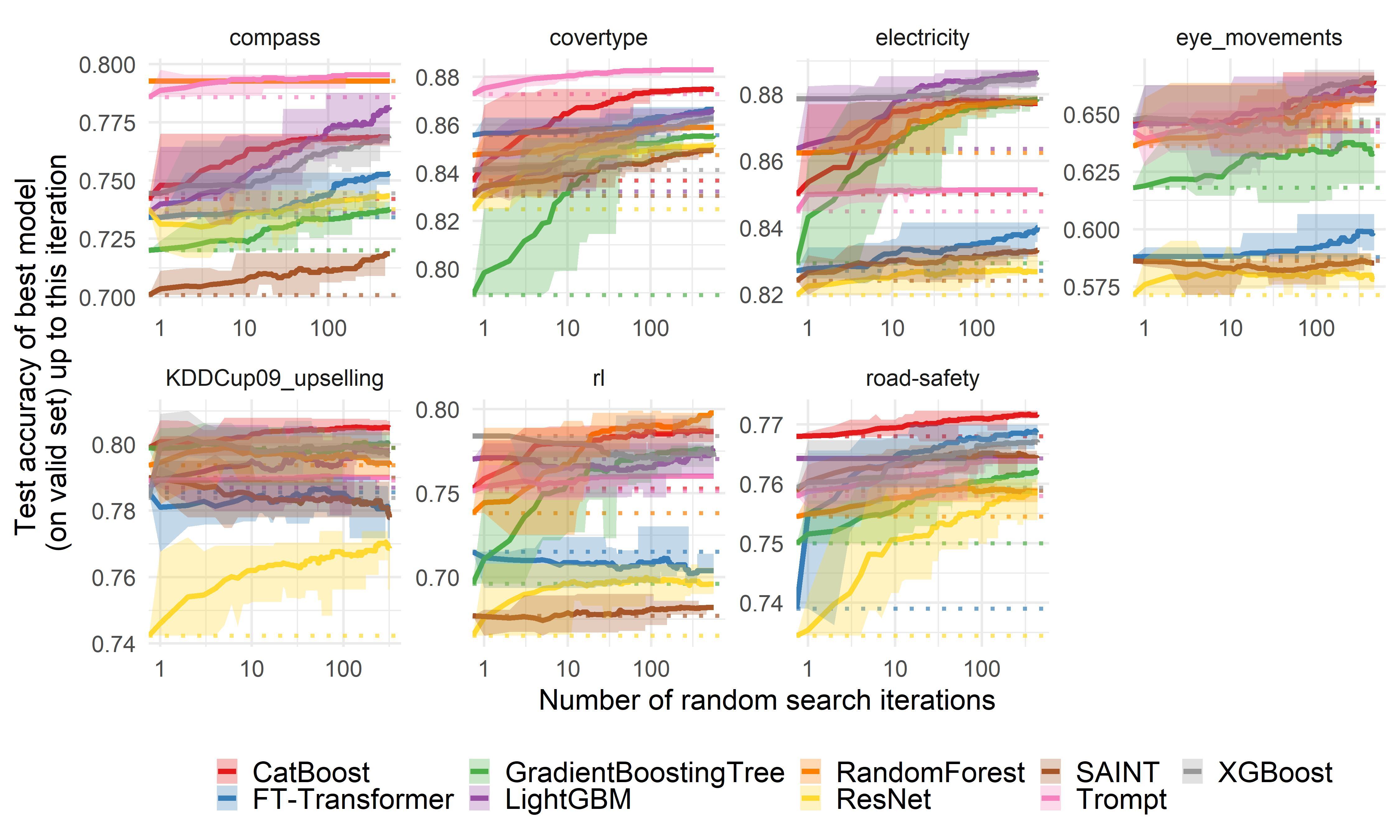
Figure 11: Benchmark on every medium-sized classification dataset with heterogeneous features.

Furthermore, individual figures illustrating the performance of Trompt on medium-sized tasks are provided in Figure 11 for heterogeneous features, and in Figure 12 for numerical features only. The individual figures for large-sized tasks can be found in Figure 13 for heterogeneous features, and in Figure 14 for numerical features only.

The evaluation results consistently demonstrate that Trompt outperforms state-of-the-art deep neural networks (FT-Transformer and SAINT) across all classification tasks (refer to Tables 9, 10, 11, 12 and 13). Moreover, Trompt’s default rankings consistently yield better performance than the searched rankings, indicating its strength in default configurations without tuning. Remarkably, in a large-sized task with numerical features only, Trompt even surpasses tree-based models (refer to Table 13).

Table 9: The performance of medium-sized classification task (heterogeneous features).

	A1	A2	A3	A4	A5	A6	A7	Ranking
Default
Trompt (ours)	$78.91\%$	$78.59\%$	$87.29\%$	$84.50\%$	$64.25\%$	$75.13\%$	$75.80\%$	$3.71\pm 1.78$
FT-Transformer	$78.56\%$	$73.43\%$	$85.57\%$	$82.71\%$	$58.79\%$	$71.52\%$	$73.90\%$	$6.29\pm 2.00$
ResNet	$74.24\%$	$73.78\%$	$82.49\%$	$81.99\%$	$57.14\%$	$66.51\%$	$73.45\%$	$8.29\pm 2.92$
SAINT	$79.00\%$	$70.09\%$	$83.04\%$	$82.42\%$	$58.62\%$	$67.69\%$	$75.89\%$	$6.86\pm 2.55$
CatBoost	$79.90\%$	$74.22\%$	$83.69\%$	$85.01\%$	$64.62\%$	$75.29\%$	$76.80\%$	$2.93\pm 2.55$
LightGBM	$78.70\%$	$73.63\%$	$83.23\%$	$86.37\%$	$64.48\%$	$77.04\%$	$76.43\%$	$3.86\pm 1.93$
XGBoost	$78.39\%$	$74.46\%$	$84.13\%$	$87.86\%$	$64.77\%$	$78.42\%$	$75.94\%$	$3.00\pm 2.92$
RandomForest	$79.38\%$	$79.28\%$	$84.75\%$	$86.24\%$	$63.62\%$	$73.82\%$	$75.45\%$	$3.71\pm 1.86$
GradientBoostingTree	$79.90\%$	$72.01\%$	$78.92\%$	$82.94\%$	$61.81\%$	$69.60\%$	$75.00\%$	$6.36\pm 2.51$
Searched
Trompt (ours)	$79.00\%$	$79.55\%$	$88.29\%$	$85.13\%$	$64.29\%$	$76.02\%$	$76.38\%$	$4.43\pm 2.20$
FT-Transformer	$78.00\%$	$75.30\%$	$86.64\%$	$84.01\%$	$59.85\%$	$70.38\%$	$76.86\%$	$5.57\pm 2.19$
ResNet	$76.87\%$	$74.35\%$	$85.17\%$	$82.68\%$	$57.82\%$	$69.59\%$	$75.85\%$	$8.43\pm 2.73$
SAINT	$77.80\%$	$71.87\%$	$84.95\%$	$83.32\%$	$58.54\%$	$68.20\%$	$76.43\%$	$7.86\pm 2.64$
CatBoost	$80.50\%$	$76.87\%$	$87.48\%$	$87.73\%$	$66.48\%$	$78.67\%$	$77.16\%$	$2.43\pm 2.71$
LightGBM	$79.81\%$	$78.15\%$	$86.62\%$	$88.64\%$	$66.14\%$	$77.69\%$	$76.43\%$	$3.14\pm 2.05$
XGBoost	$79.69\%$	$76.83\%$	$86.25\%$	$88.52\%$	$66.57\%$	$77.18\%$	$76.69\%$	$3.57\pm 1.93$
RandomForest	$79.38\%$	$79.28\%$	$85.89\%$	$87.76\%$	$65.70\%$	$79.79\%$	$75.88\%$	$4.29\pm 2.27$
GradientBoostingTree	$80.01\%$	$73.77\%$	$85.55\%$	$87.85\%$	$63.30\%$	$77.58\%$	$76.23\%$	$5.29\pm 2.17$

Table 10: The performance of medium-sized classification task (numerical features only) (1).

	B1	B2	B3	B4	B5	B6	B7	B8
Default
Trompt (ours)	$69.26\%$	$86.30\%$	$93.82\%$	$79.36\%$	$89.09\%$	$82.68\%$	$75.84\%$	$82.89\%$
FT-Transformer	$66.94\%$	$84.42\%$	$92.80\%$	$80.09\%$	$87.40\%$	$80.42\%$	$74.32\%$	$81.24\%$
ResNet	$65.39\%$	$85.11\%$	$93.10\%$	$78.68\%$	$86.90\%$	$79.09\%$	$74.99\%$	$80.91\%$
SAINT	$69.29\%$	$85.16\%$	$93.18\%$	$79.18\%$	$87.69\%$	$78.05\%$	$76.49\%$	$81.25\%$
CatBoost	$71.30\%$	$86.14\%$	$93.64\%$	$80.45\%$	$90.21\%$	$80.16\%$	$76.95\%$	$84.48\%$
LightGBM	$70.79\%$	$85.47\%$	$93.16\%$	$80.33\%$	$90.06\%$	$79.50\%$	$77.17\%$	$84.34\%$
XGBoost	$69.25\%$	$85.31\%$	$93.29\%$	$79.81\%$	$90.30\%$	$79.87\%$	$75.91\%$	$86.11\%$
RandomForest	$70.12\%$	$85.56\%$	$92.09\%$	$79.46\%$	$88.80\%$	$81.35\%$	$76.64\%$	$84.79\%$
GradientBoostingTree	$70.49\%$	$84.44\%$	$92.16\%$	$80.27\%$	$88.00\%$	$76.85\%$	$77.52\%$	$82.16\%$
Searched
Trompt (ours)	$69.60\%$	$86.35\%$	$93.74\%$	$79.30\%$	$89.28\%$	$83.73\%$	$76.52\%$	$83.12\%$
FT-Transformer	$70.67\%$	$85.26\%$	$93.59\%$	$80.22\%$	$88.61\%$	$81.22\%$	$76.50\%$	$81.94\%$
ResNet	$69.02\%$	$85.62\%$	$93.69\%$	$79.13\%$	$87.28\%$	$80.21\%$	$76.28\%$	$80.98\%$
SAINT	$70.73\%$	$84.85\%$	$93.54\%$	$79.29\%$	$88.92\%$	$80.27\%$	$76.24\%$	$81.84\%$
CatBoost	$71.46\%$	$85.92\%$	$93.84\%$	$80.39\%$	$90.32\%$	$82.98\%$	$77.59\%$	$86.33\%$
LightGBM	$71.01\%$	$85.70\%$	$93.71\%$	$80.15\%$	$90.13\%$	$81.81\%$	$77.13\%$	$85.94\%$
XGBoost	$71.36\%$	$86.05\%$	$93.66\%$	$80.34\%$	$90.12\%$	$81.75\%$	$77.26\%$	$86.94\%$
RandomForest	$70.76\%$	$85.41\%$	$92.65\%$	$79.82\%$	$89.21\%$	$82.73\%$	$77.25\%$	$86.14\%$
GradientBoostingTree	$71.00\%$	$85.57\%$	$93.22\%$	$80.26\%$	$89.68\%$	$81.72\%$	$77.27\%$	$86.24\%$

Table 11: The performance of medium-sized classification task (numerical features only) (2).

	B9	B10	B11	B12	B13	B14	B15	Ranking
Default
Trompt (ours)	$61.60\%$	$88.05\%$	$76.89\%$	$86.61\%$	$88.67\%$	$98.49\%$	$79.07\%$	$4.07\pm 2.61$
FT-Transformer	$58.62\%$	$87.16\%$	$72.94\%$	$87.16\%$	$85.67\%$	$98.08\%$	$77.21\%$	$6.93\pm 2.06$
ResNet	$56.06\%$	$86.48\%$	$70.70\%$	$86.94\%$	$85.37\%$	$94.87\%$	$77.06\%$	$8.20\pm 2.05$
SAINT	$57.18\%$	$88.19\%$	$76.04\%$	$88.32\%$	$85.28\%$	$97.04\%$	$75.90\%$	$6.20\pm 2.13$
CatBoost	$63.87\%$	$88.59\%$	$77.85\%$	$87.98\%$	$87.44\%$	$98.46\%$	$78.58\%$	$2.47\pm 2.03$
LightGBM	$64.39\%$	$88.43\%$	$77.27\%$	$87.43\%$	$86.90\%$	$98.38\%$	$79.81\%$	$3.27\pm 1.82$
XGBoost	$64.75\%$	$88.16\%$	$76.00\%$	$87.31\%$	$87.05\%$	$98.35\%$	$79.78\%$	$4.13\pm 1.97$
RandomForest	$63.16\%$	$87.92\%$	$76.34\%$	$88.32\%$	$88.01\%$	$98.10\%$	$80.30\%$	$3.93\pm 2.16$
GradientBoostingTree	$62.33\%$	$87.68\%$	$76.17\%$	$88.32\%$	$84.26\%$	$96.71\%$	$77.09\%$	$5.80\pm 2.52$
Searched
Trompt (ours)	$62.71\%$	$88.46\%$	$76.99\%$	$87.25\%$	$88.67\%$	$98.38\%$	$78.58\%$	$4.80\pm 2.47$
FT-Transformer	$58.30\%$	$88.15\%$	$76.43\%$	$89.12\%$	$85.66\%$	$98.45\%$	$76.74\%$	$6.47\pm 2.41$
ResNet	$57.03\%$	$87.54\%$	$74.63\%$	$88.23\%$	$85.87\%$	$94.86\%$	$77.41\%$	$7.73\pm 2.50$
SAINT	$58.90\%$	$88.27\%$	$77.22\%$	$89.05\%$	$85.39\%$	$98.12\%$	$76.87\%$	$6.93\pm 2.22$
CatBoost	$65.07\%$	$88.54\%$	$77.95\%$	$88.02\%$	$88.83\%$	$98.47\%$	$79.89\%$	$1.93\pm 2.36$
LightGBM	$65.43\%$	$88.62\%$	$77.70\%$	$88.18\%$	$87.60\%$	$98.21\%$	$79.55\%$	$3.53\pm 1.44$
XGBoost	$65.83\%$	$88.83\%$	$77.83\%$	$88.12\%$	$86.81\%$	$98.09\%$	$79.46\%$	$3.20\pm 2.22$
RandomForest	$65.04\%$	$87.80\%$	$77.27\%$	$87.95\%$	$88.45\%$	$98.20\%$	$78.96\%$	$5.33\pm 1.88$
GradientBoostingTree	$63.04\%$	$88.22\%$	$77.17\%$	$88.32\%$	$86.68\%$	$98.06\%$	$78.56\%$	$5.07\pm 1.77$

Table 12: The performance of large-sized classification task (heterogeneous features).

	$\mathbb{A}$1	$\mathbb{A}$2	Ranking
Default
Trompt (ours)	$92.76\%$	$78.36\%$	$1.50\pm 4.36$
FT-Transformer	$93.17\%$	$76.09\%$	$4.50\pm 3.61$
ResNet	$89.45\%$	$76.53\%$	$6.00\pm 2.25$
SAINT	$91.23\%$	$77.31\%$	$4.50\pm 1.73$
CatBoost	$88.27\%$	$78.21\%$	$4.50\pm 1.73$
LightGBM	$84.76\%$	$77.97\%$	$6.00\pm 2.84$
XGBoost	$87.81\%$	$78.22\%$	$4.50\pm 2.65$
RandomForest	$90.66\%$	$77.67\%$	$4.50\pm 1.00$
GradientBoostingTree	$79.46\%$	$75.19\%$	$9.00\pm 4.62$
Searched
Trompt (ours)	$93.95\%$	$78.44\%$	$3.50\pm 3.40$
FT-Transformer	$93.61\%$	$78.92\%$	$3.50\pm 2.36$
ResNet	$92.27\%$	$78.40\%$	$8.00\pm 3.61$
SAINT	$92.54\%$	$77.96\%$	$8.50\pm 4.36$
CatBoost	$93.70\%$	$80.15\%$	$1.50\pm 4.36$
LightGBM	$93.25\%$	$79.75\%$	$4.00\pm 1.32$
XGBoost	$93.07\%$	$79.91\%$	$4.00\pm 2.18$
RandomForest	$93.30\%$	$78.13\%$	$6.00\pm 2.47$
GradientBoostingTree	$92.99\%$	$78.59\%$	$6.00\pm 1.76$

Table 13: The performance of large-sized classification task (numerical features only).

	$\mathbb{B}$1	$\mathbb{B}$2	$\mathbb{B}$3	$\mathbb{B}$4	Ranking
Default
Trompt (ours)	$72.13\%$	$94.68\%$	$90.04\%$	$79.54\%$	$1.38\pm 3.44$
FT-Transformer	$69.60\%$	$94.03\%$	$89.83\%$	$75.86\%$	$6.00\pm 2.96$
ResNet	$69.88\%$	$94.09\%$	$88.01\%$	$73.58\%$	$6.00\pm 2.78$
SAINT	$71.81\%$	$94.36\%$	$86.94\%$	$78.60\%$	$3.75\pm 1.82$
CatBoost	$72.61\%$	$94.32\%$	$83.77\%$	$79.54\%$	$2.88\pm 3.01$
LightGBM	$72.12\%$	$93.71\%$	$80.71\%$	$78.70\%$	$5.00\pm 2.17$
XGBoost	$71.64\%$	$93.67\%$	$83.61\%$	$78.28\%$	$6.00\pm 1.50$
RandomForest	$71.58\%$	$93.08\%$	$87.67\%$	$77.97\%$	$6.00\pm 1.80$
GradientBoostingTree	$71.03\%$	$92.25\%$	$76.98\%$	$77.18\%$	$8.00\pm 3.29$
Searched
Trompt (ours)	$72.86\%$	$94.36\%$	$91.27\%$	$79.88\%$	$3.25\pm 2.97$
FT-Transformer	$72.86\%$	$94.42\%$	$90.57\%$	$79.59\%$	$3.25\pm 2.07$
ResNet	$72.29\%$	$94.46\%$	$89.36\%$	$78.11\%$	$6.75\pm 3.49$
SAINT	$72.65\%$	$94.45\%$	$89.53\%$	$79.30\%$	$5.50\pm 1.67$
CatBoost	$72.99\%$	$94.55\%$	$90.19\%$	$79.89\%$	$1.75\pm 3.49$
LightGBM	$72.55\%$	$94.39\%$	$89.71\%$	$79.32\%$	$6.00\pm 0.89$
XGBoost	$72.81\%$	$94.40\%$	$89.32\%$	$79.67\%$	$5.25\pm 2.30$
RandomForest	$71.98\%$	$93.53\%$	$90.59\%$	$78.85\%$	$7.00\pm 3.96$
GradientBoostingTree	$72.49\%$	$94.07\%$	$89.79\%$	$79.34\%$	$6.25\pm 1.95$

Figure 12: Benchmark on every medium-sized classification dataset with numerical features only.

Figure 13: Benchmark on every large-sized classification dataset with heterogeneous features.

Figure 14: Benchmark on every large-sized classification dataset with numerical features only.

B.1.2 Regression

The evaluation results for medium-sized regression datasets are presented in Tables 14 and 15 for heterogeneous features, and in Tables 16, 17 and 18 for numerical features only.

For large-sized regression datasets, the results can be found in Table 19 for heterogeneous features, and in Table 20 for numerical features only.

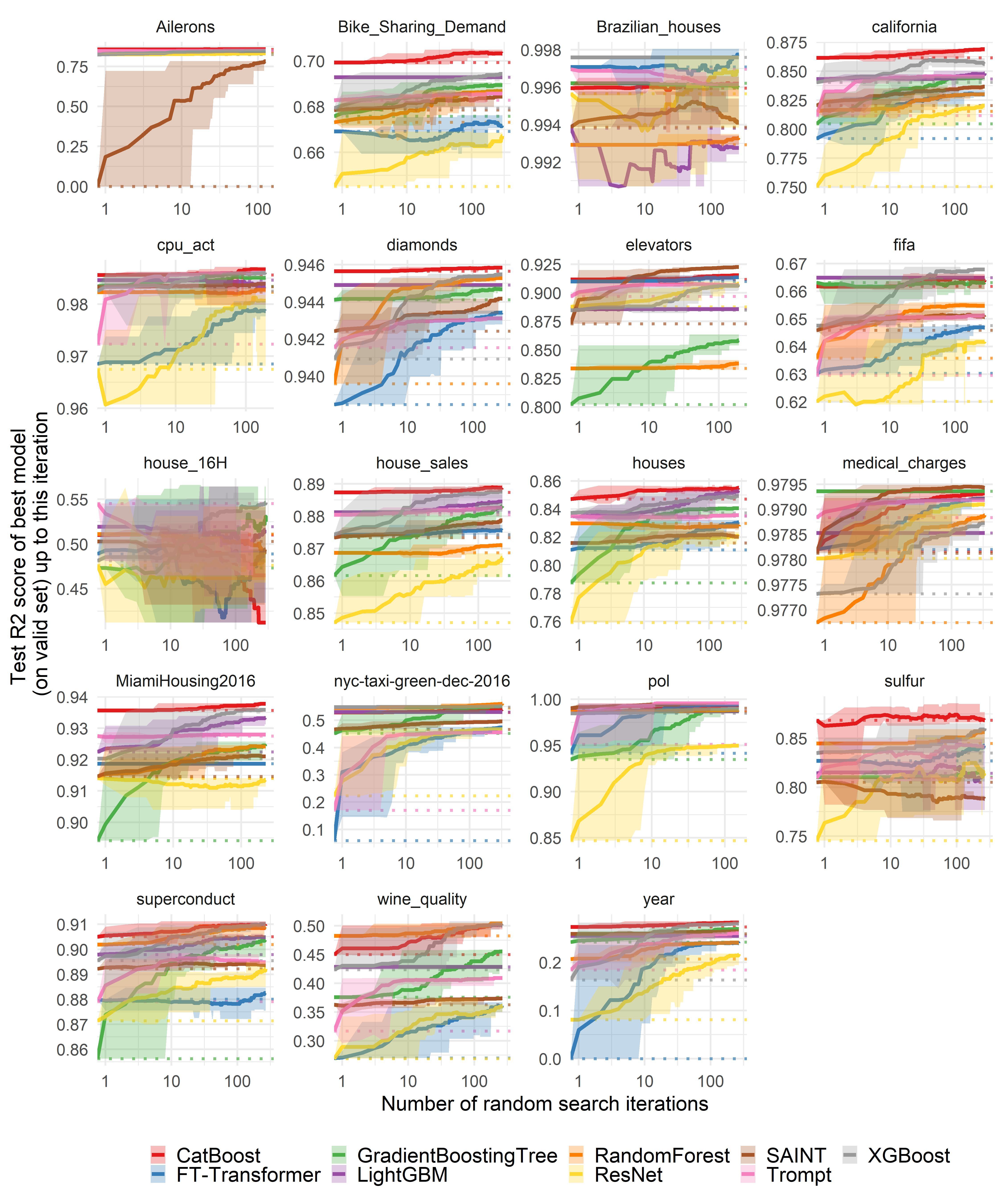
Figure 16: Benchmark on every medium-sized regression dataset with numerical features only.

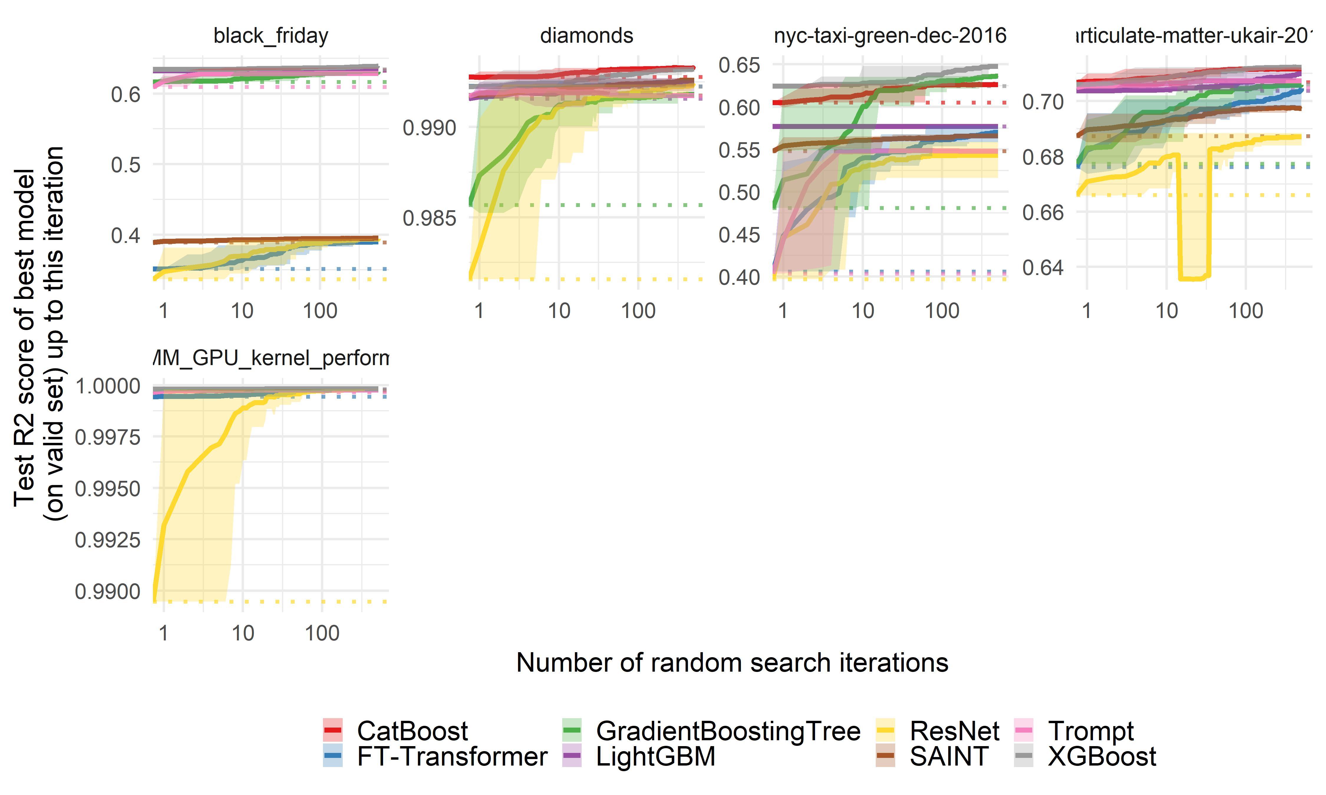
Figure 17: Benchmark on every large-sized regression dataset with heterogeneous features.

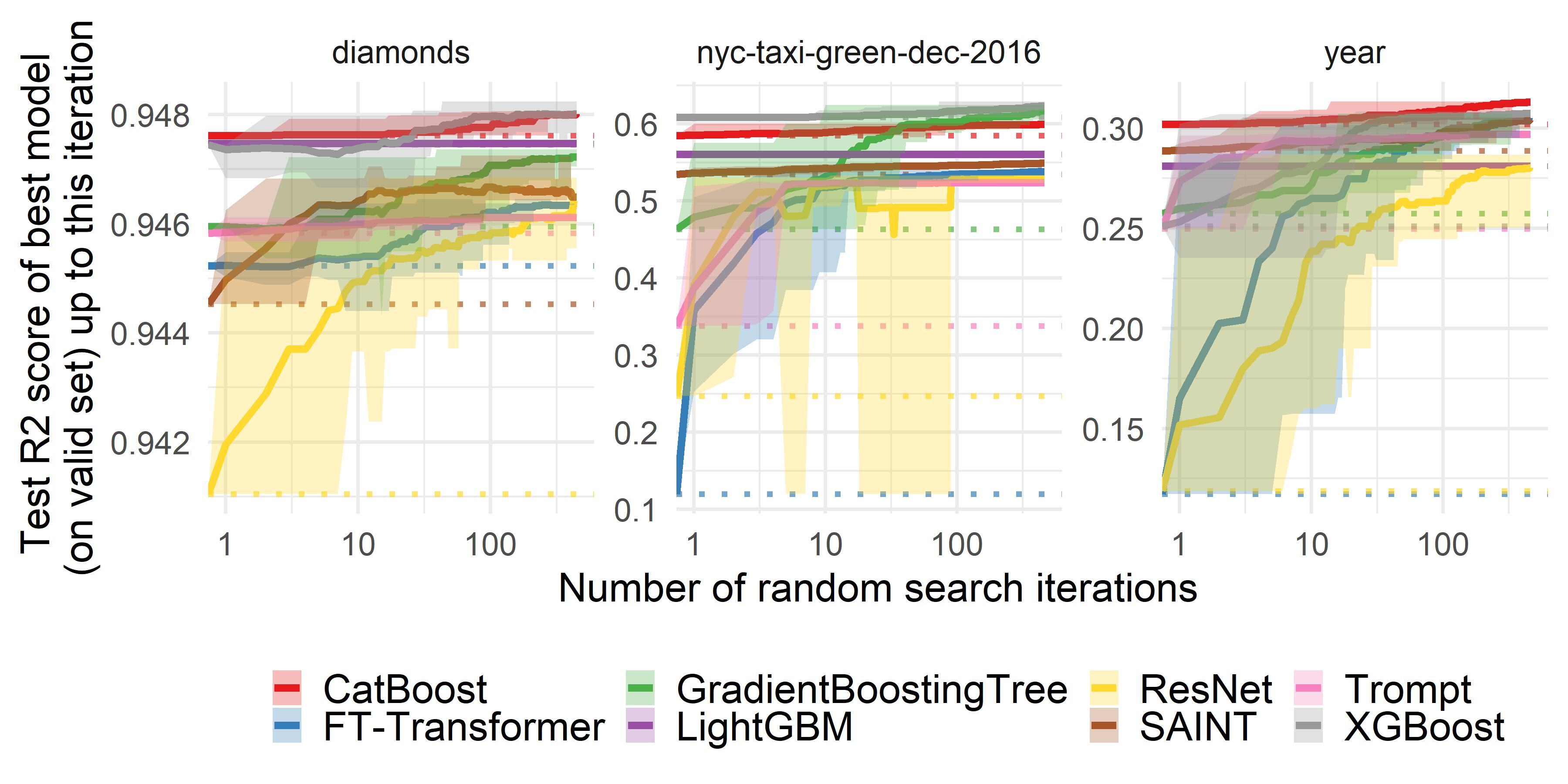
Figure 18: Benchmark on every large-sized regression dataset with numerical features only.

Furthermore, individual figures illustrating the performance of Trompt on medium-sized regression tasks are provided in Figure 15 for heterogeneous features, and in Figure 16 for numerical features only. The individual figures for large-sized tasks can be found in Figure 17 for heterogeneous features, and in Figure 18 for numerical features only.

The evaluation results consistently demonstrate that Trompt outperforms state-of-the-art deep neural networks (SAINT and FT-Transformer) on medium-sized regression tasks (refer to Tables 14, 15, 16, 17 and 18). However, Trompt’s performance is slightly inferior to other deep neural networks on large-sized datasets (refer to Tables 19 and 20). Nevertheless, it is worth noting that the performance of Trompt remains consistently competitive when considering all benchmark results.

Table 14: The performance of medium-sized regression task (heterogeneous features) (1).

	C1	C2	C3	C4	C5	C6	C7	C8
Default
Trompt (ours)	$93.93\%$	$99.63\%$	$54.09\%$	$8.71\%$	$99.96\%$	$94.70\%$	$57.94\%$	$98.88\%$
FT-Transformer	$93.21\%$	$88.00\%$	$54.24\%$	$0.00\%$	$99.96\%$	$93.99\%$	$31.46\%$	$98.84\%$
ResNet	$89.90\%$	$87.47\%$	$51.99\%$	$0.00\%$	$99.72\%$	$91.09\%$	$10.79\%$	$98.46\%$
SAINT	$92.50\%$	$99.20\%$	$54.25\%$	$11.23\%$	$99.96\%$	$95.10\%$	$40.72\%$	$98.47\%$
CatBoost	$94.21\%$	$99.59\%$	$56.33\%$	$15.16\%$	$99.97\%$	$98.01\%$	$61.70\%$	$99.11\%$
LightGBM	$94.02\%$	$99.38\%$	$54.77\%$	$14.41\%$	$99.97\%$	$98.23\%$	$61.68\%$	$99.01\%$
XGBoost	$93.93\%$	$99.76\%$	$49.71\%$	$6.64\%$	$99.97\%$	$97.59\%$	$58.93\%$	$98.96\%$
RandomForest	$93.61\%$	$99.30\%$	$50.78\%$	$13.16\%$	$99.98\%$	$98.00\%$	$55.85\%$	$98.79\%$
GradientBoostingTree	$84.15\%$	$99.62\%$	$57.17\%$	$15.30\%$	$99.97\%$	$98.27\%$	$61.34\%$	$98.42\%$
Searched
Trompt (ours)	$94.50\%$	$99.75\%$	$56.87\%$	$13.05\%$	$99.96\%$	$97.93\%$	$60.17\%$	$98.99\%$
FT-Transformer	$93.58\%$	$88.12\%$	$54.90\%$	$14.05\%$	$99.97\%$	$97.63\%$	$37.93\%$	$98.96\%$
ResNet	$93.65\%$	$87.83\%$	$54.47\%$	$12.95\%$	$99.96\%$	$97.83\%$	$35.56\%$	$98.79\%$
SAINT	$93.89\%$	$99.51\%$	$55.14\%$	$13.90\%$	$99.97\%$	$94.59\%$	$58.72\%$	$98.72\%$
CatBoost	$94.87\%$	$99.60\%$	$57.74\%$	$16.54\%$	$99.97\%$	$98.33\%$	$61.79\%$	$99.18\%$
LightGBM	$94.37\%$	$99.42\%$	$55.58\%$	$14.41\%$	$99.97\%$	$98.23\%$	$61.68\%$	$99.07\%$
XGBoost	$94.62\%$	$99.76\%$	$56.87\%$	$16.21\%$	$99.98\%$	$98.30\%$	$61.88\%$	$99.12\%$
RandomForest	$93.79\%$	$99.34\%$	$57.55\%$	$14.94\%$	$99.98\%$	$98.07\%$	$60.91\%$	$98.79\%$
GradientBoostingTree	$94.07\%$	$99.46\%$	$57.53\%$	$15.27\%$	$99.98\%$	$98.13\%$	$61.54\%$	$98.98\%$

Table 15: The performance of medium-sized regression task (heterogeneous features) (2).

	C9	C10	C11	C12	C13	Ranking
Default
Trompt (ours)	$89.02\%$	$9.61\%$	$64.94\%$	$99.95\%$	$0.64\%$	$5.38\pm 2.02$
FT-Transformer	$87.38\%$	$12.38\%$	$65.43\%$	$99.94\%$	$0.00\%$	$6.88\pm 1.74$
ResNet	$86.45\%$	$0.00\%$	$65.23\%$	$98.70\%$	$0.00\%$	$8.35\pm 2.13$
SAINT	$88.01\%$	$17.48\%$	$64.80\%$	$99.98\%$	$0.00\%$	$6.31\pm 1.54$
CatBoost	$89.75\%$	$54.63\%$	$69.16\%$	$99.99\%$	$4.97\%$	$2.15\pm 2.13$
LightGBM	$89.05\%$	$54.48\%$	$68.74\%$	$99.99\%$	$4.91\%$	$3.00\pm 1.74$
XGBoost	$88.34\%$	$56.99\%$	$66.16\%$	$100.00\%$	$0.00\%$	$4.08\pm 2.46$
RandomForest	$87.44\%$	$56.18\%$	$65.44\%$	$100.00\%$	$5.92\%$	$4.23\pm 2.27$
GradientBoostingTree	$86.93\%$	$46.90\%$	$67.17\%$	$99.94\%$	$0.00\%$	$4.62\pm 2.92$
Searched
Trompt (ours)	$89.16\%$	$48.04\%$	$66.33\%$	$99.99\%$	$3.59\%$	$5.77\pm 1.98$
FT-Transformer	$88.85\%$	$50.44\%$	$67.18\%$	$99.90\%$	$3.18\%$	$7.23\pm 1.70$
ResNet	$88.10\%$	$42.42\%$	$65.50\%$	$99.76\%$	$2.11\%$	$8.31\pm 2.08$
SAINT	$89.18\%$	$36.42\%$	$66.93\%$	$99.99\%$	$1.21\%$	$7.00\pm 1.98$
CatBoost	$89.84\%$	$56.79\%$	$69.33\%$	$100.00\%$	$9.08\%$	$2.00\pm 2.24$
LightGBM	$89.33\%$	$54.48\%$	$68.74\%$	$100.00\%$	$4.91\%$	$4.31\pm 1.18$
XGBoost	$89.65\%$	$57.82\%$	$69.08\%$	$100.00\%$	$8.01\%$	$2.15\pm 1.74$
RandomForest	$87.50\%$	$58.48\%$	$67.44\%$	$100.00\%$	$9.52\%$	$4.31\pm 2.80$
GradientBoostingTree	$89.05\%$	$57.29\%$	$68.30\%$	$100.00\%$	$5.54\%$	$3.92\pm 1.35$

Table 16: The performance of medium-sized regression task (numerical features only) (1).

	D1	D2	D3	D4	D5	D6	D7
Default
Trompt (ours)	$84.80\%$	$68.29\%$	$99.70\%$	$92.75\%$	$81.17\%$	$97.23\%$	$94.15\%$
FT-Transformer	$83.80\%$	$66.92\%$	$99.71\%$	$91.87\%$	$79.20\%$	$96.85\%$	$93.85\%$
ResNet	$82.54\%$	$64.52\%$	$99.57\%$	$91.41\%$	$75.06\%$	$96.75\%$	$nan$
SAINT	$0.00\%$	$67.85\%$	$99.39\%$	$91.46\%$	$82.04\%$	$98.33\%$	$94.24\%$
CatBoost	$85.76\%$	$69.93\%$	$99.60\%$	$93.56\%$	$86.16\%$	$98.56\%$	$94.57\%$
LightGBM	$84.68\%$	$69.28\%$	$99.38\%$	$92.25\%$	$84.33\%$	$98.46\%$	$94.49\%$
XGBoost	$82.58\%$	$67.93\%$	$99.76\%$	$92.03\%$	$84.04\%$	$98.25\%$	$94.09\%$
RandomForest	$83.71\%$	$67.32\%$	$99.29\%$	$91.41\%$	$81.54\%$	$98.23\%$	$93.96\%$
GradientBoostingTree	$83.95\%$	$67.58\%$	$99.62\%$	$89.42\%$	$80.46\%$	$98.34\%$	$94.41\%$
Searched
Trompt (ours)	$85.08\%$	$68.57\%$	$99.62\%$	$92.80\%$	$84.53\%$	$98.61\%$	$94.31\%$
FT-Transformer	$83.90\%$	$67.17\%$	$99.77\%$	$91.87\%$	$83.00\%$	$97.87\%$	$94.34\%$
ResNet	$83.21\%$	$66.71\%$	$99.69\%$	$91.36\%$	$82.03\%$	$98.07\%$	$nan$
SAINT	$78.31\%$	$68.44\%$	$99.41\%$	$92.10\%$	$83.67\%$	$98.39\%$	$94.42\%$
CatBoost	$85.92\%$	$70.31\%$	$99.62\%$	$93.78\%$	$86.90\%$	$98.67\%$	$94.59\%$
LightGBM	$84.68\%$	$69.28\%$	$99.28\%$	$93.33\%$	$84.80\%$	$98.31\%$	$94.49\%$
XGBoost	$84.58\%$	$69.43\%$	$99.76\%$	$93.59\%$	$85.64\%$	$98.61\%$	$94.55\%$
RandomForest	$83.75\%$	$68.69\%$	$99.33\%$	$92.42\%$	$83.02\%$	$98.28\%$	$94.53\%$
GradientBoostingTree	$84.25\%$	$68.94\%$	$99.60\%$	$92.43\%$	$84.48\%$	$98.51\%$	$94.47\%$

Table 17: The performance of medium-sized regression task (numerical features only) (2).

	D8	D9	D10	D11	D12	D13	D14
Default
Trompt (ours)	$89.69\%$	$62.96\%$	$54.53\%$	$88.04\%$	$83.52\%$	$97.88\%$	$16.99\%$
FT-Transformer	$91.01\%$	$63.03\%$	$48.90\%$	$87.42\%$	$81.10\%$	$97.82\%$	$5.86\%$
ResNet	$88.77\%$	$62.01\%$	$47.62\%$	$84.71\%$	$75.92\%$	$97.80\%$	$22.34\%$
SAINT	$87.30\%$	$64.59\%$	$50.30\%$	$87.34\%$	$81.59\%$	$97.81\%$	$46.65\%$
CatBoost	$91.17\%$	$66.18\%$	$51.01\%$	$88.73\%$	$84.72\%$	$97.82\%$	$52.91\%$
LightGBM	$88.59\%$	$66.49\%$	$51.95\%$	$88.12\%$	$83.51\%$	$97.85\%$	$53.06\%$
XGBoost	$88.48\%$	$64.75\%$	$48.14\%$	$87.43\%$	$83.74\%$	$97.73\%$	$54.87\%$
RandomForest	$83.37\%$	$63.58\%$	$51.12\%$	$86.87\%$	$82.99\%$	$97.67\%$	$54.54\%$
GradientBoostingTree	$80.22\%$	$66.31\%$	$47.33\%$	$86.16\%$	$78.74\%$	$97.94\%$	$45.15\%$
Searched
Trompt (ours)	$90.69\%$	$65.13\%$	$46.50\%$	$88.27\%$	$83.57\%$	$97.92\%$	$45.57\%$
FT-Transformer	$91.37\%$	$64.69\%$	$48.67\%$	$87.56\%$	$83.05\%$	$97.92\%$	$47.43\%$
ResNet	$90.82\%$	$64.19\%$	$48.16\%$	$86.72\%$	$82.08\%$	$97.91\%$	$46.78\%$
SAINT	$92.27\%$	$65.06\%$	$49.40\%$	$87.87\%$	$82.03\%$	$97.94\%$	$49.58\%$
CatBoost	$91.56\%$	$66.39\%$	$41.22\%$	$88.89\%$	$85.53\%$	$97.93\%$	$54.06\%$
LightGBM	$88.59\%$	$66.49\%$	$51.60\%$	$88.45\%$	$85.33\%$	$97.85\%$	$53.06\%$
XGBoost	$90.67\%$	$66.79\%$	$54.63\%$	$88.76\%$	$84.95\%$	$97.87\%$	$55.23\%$
RandomForest	$83.82\%$	$65.47\%$	$49.15\%$	$87.10\%$	$82.77\%$	$97.89\%$	$56.04\%$
GradientBoostingTree	$85.84\%$	$66.32\%$	$52.49\%$	$88.32\%$	$84.07\%$	$97.94\%$	$55.21\%$

Table 18: The performance of medium-sized regression task (numerical features only) (3).

	D15	D16	D17	D18	D19	Ranking
Default
Trompt (ours)	$95.13\%$	$80.96\%$	$87.91\%$	$31.68\%$	$18.41\%$	$4.68\pm 2.29$
FT-Transformer	$94.16\%$	$82.70\%$	$88.01\%$	$26.98\%$	$0.00\%$	$6.21\pm 2.29$
ResNet	$84.68\%$	$74.54\%$	$87.14\%$	$26.86\%$	$8.13\%$	$8.06\pm 2.08$
SAINT	$99.04\%$	$80.52\%$	$89.22\%$	$36.25\%$	$25.92\%$	$5.32\pm 1.86$
CatBoost	$98.63\%$	$86.85\%$	$90.51\%$	$45.00\%$	$27.34\%$	$2.05\pm 2.16$
LightGBM	$98.70\%$	$81.43\%$	$89.79\%$	$42.86\%$	$25.50\%$	$3.05\pm 1.89$
XGBoost	$98.50\%$	$83.49\%$	$89.55\%$	$42.37\%$	$16.33\%$	$4.47\pm 2.04$
RandomForest	$98.67\%$	$84.47\%$	$90.20\%$	$48.28\%$	$20.69\%$	$5.26\pm 2.40$
GradientBoostingTree	$93.49\%$	$81.04\%$	$85.62\%$	$37.57\%$	$24.21\%$	$5.84\pm 2.60$
Searched
Trompt (ours)	$99.58\%$	$84.15\%$	$89.49\%$	$40.91\%$	$26.03\%$	$5.11\pm 1.97$
FT-Transformer	$99.44\%$	$84.26\%$	$88.26\%$	$36.07\%$	$23.96\%$	$6.37\pm 2.48$
ResNet	$94.99\%$	$81.45\%$	$89.22\%$	$36.11\%$	$21.73\%$	$7.61\pm 2.31$
SAINT	$99.56\%$	$78.81\%$	$89.37\%$	$37.38\%$	$26.45\%$	$5.79\pm 2.46$
CatBoost	$99.24\%$	$86.84\%$	$90.94\%$	$50.11\%$	$28.26\%$	$2.26\pm 2.46$
LightGBM	$98.70\%$	$81.31\%$	$90.48\%$	$42.86\%$	$25.50\%$	$4.84\pm 2.25$
XGBoost	$98.97\%$	$86.03\%$	$91.02\%$	$50.06\%$	$28.04\%$	$2.79\pm 2.11$
RandomForest	$98.87\%$	$85.64\%$	$90.89\%$	$50.43\%$	$24.09\%$	$5.58\pm 2.33$
GradientBoostingTree	$98.91\%$	$81.31\%$	$90.36\%$	$45.55\%$	$26.94\%$	$4.58\pm 1.69$

Table 19: The performance of large-sized regression task (heterogeneous features).

	$\mathbb{C}$1	$\mathbb{C}$2	$\mathbb{C}$3	$\mathbb{C}$4	$\mathbb{C}$5	Ranking
Default
Trompt (ours)	$99.96\%$	$60.97\%$	$99.17\%$	$40.35\%$	$70.48\%$	$5.20\pm 1.50$
FT-Transformer	$99.94\%$	$35.14\%$	$99.23\%$	$40.61\%$	$67.61\%$	$5.80\pm 2.48$
ResNet	$98.95\%$	$33.70\%$	$98.16\%$	$39.71\%$	$66.60\%$	$8.00\pm 2.86$
SAINT	$99.97\%$	$38.91\%$	$99.18\%$	$54.80\%$	$68.74\%$	$4.80\pm 0.75$
CatBoost	$99.98\%$	$63.32\%$	$99.28\%$	$60.50\%$	$70.68\%$	$1.80\pm 2.25$
LightGBM	$99.98\%$	$63.24\%$	$99.16\%$	$57.69\%$	$70.37\%$	$3.60\pm 1.67$
XGBoost	$99.98\%$	$63.45\%$	$99.22\%$	$62.44\%$	$70.60\%$	$1.60\pm 2.73$
RandomForest	$-$	$-$	$-$	$-$	$-$	$-$
GradientBoostingTree	$99.98\%$	$61.65\%$	$98.57\%$	$48.09\%$	$67.73\%$	$5.20\pm 1.36$
Searched
Trompt (ours)	$99.98\%$	$62.86\%$	$99.18\%$	$54.79\%$	$70.73\%$	$6.20\pm 2.26$
FT-Transformer	$99.98\%$	$39.00\%$	$99.26\%$	$57.02\%$	$70.45\%$	$5.80\pm 1.75$
ResNet	$99.98\%$	$39.38\%$	$99.23\%$	$54.30\%$	$68.71\%$	$6.40\pm 2.88$
SAINT	$99.98\%$	$39.53\%$	$99.26\%$	$56.58\%$	$69.73\%$	$5.20\pm 1.55$
CatBoost	$99.98\%$	$63.62\%$	$99.33\%$	$62.64\%$	$71.17\%$	$2.60\pm 2.25$
LightGBM	$99.98\%$	$63.24\%$	$99.24\%$	$57.69\%$	$70.99\%$	$4.60\pm 1.86$
XGBoost	$99.98\%$	$63.90\%$	$99.32\%$	$64.79\%$	$71.22\%$	$1.20\pm 2.80$
RandomForest	$-$	$-$	$-$	$-$	$-$	$-$
GradientBoostingTree	$99.98\%$	$63.06\%$	$99.18\%$	$63.62\%$	$70.58\%$	$4.00\pm 2.07$

Table 20: The performance of large-sized regression task (numerical features only).

	$\mathbb{D}$1	$\mathbb{D}$2	$\mathbb{D}$3	Ranking
Default
Trompt (ours)	$94.58\%$	$33.79\%$	$24.98\%$	$5.67\pm 1.41$
FT-Transformer	$94.52\%$	$11.98\%$	$11.72\%$	$7.33\pm 3.07$
ResNet	$94.10\%$	$24.69\%$	$11.88\%$	$7.33\pm 2.95$
SAINT	$94.45\%$	$53.44\%$	$28.87\%$	$4.33\pm 2.06$
CatBoost	$94.76\%$	$58.47\%$	$30.20\%$	$1.33\pm 3.37$
LightGBM	$94.75\%$	$56.07\%$	$28.10\%$	$2.67\pm 2.22$
XGBoost	$94.74\%$	$60.87\%$	$25.12\%$	$3.00\pm 2.22$
RandomForest	$-$	$-$	$-$	$-$
GradientBoostingTree	$94.59\%$	$46.35\%$	$25.74\%$	$4.33\pm 0.48$
Searched
Trompt (ours)	$94.61\%$	$52.42\%$	$29.71\%$	$7.33\pm 3.30$
FT-Transformer	$94.63\%$	$53.82\%$	$30.51\%$	$5.67\pm 1.83$
ResNet	$94.64\%$	$52.84\%$	$28.01\%$	$7.00\pm 2.63$
SAINT	$94.65\%$	$54.94\%$	$30.46\%$	$5.00\pm 0.50$
CatBoost	$94.80\%$	$59.97\%$	$31.30\%$	$2.00\pm 2.63$
LightGBM	$94.75\%$	$56.07\%$	$28.10\%$	$4.67\pm 1.71$
XGBoost	$94.80\%$	$62.36\%$	$30.75\%$	$1.33\pm 3.37$
RandomForest	$-$	$-$	$-$	$-$
GradientBoostingTree	$94.72\%$	$61.72\%$	$30.73\%$	$3.00\pm 1.71$

Figure 15: Benchmark on every medium-sized regression dataset with heterogeneous features.

B.2 Datasets chosen by FT-Transformer

In this section, we further investigate the performance of Trompt on datasets selected by FT-Transformer (Gorishniy et al., 2021), which encompass different domains, task types, and sizes. To ensure a fair comparison, we adjust the model sizes of Trompt to match those of FT-Transformer by reducing the dimensions of its hidden layers.

It’s important to note that due to limited computing resources, Trompt did not undergo hyperparameter search. Instead, we obtained the performance of FT-Transformer from its original paper. In terms of the learning strategy, Trompt was trained for 100 epochs, and the performance was evaluated using the checkpoint at the 100th epoch. This approach was adopted as we observed that the datasets chosen by FT-Transformer are often large, making overfitting less likely.

As shown in Table 21, Trompt generally achieves comparable or slightly inferior performance when compared to the default hyperparameter settings of FT-Transformer on the datasets specifically chosen by FT-Transformer. It is important to note that the reported performance is an average result based on three random seeds.

Table 21: The performance on datasets chosen by FT-Transformer.

Dataset	Metric	Trompt (ours)	FT (Default)	FT (Tune)	#Parameters (Trompt)	#Parameters (FT)
CA	RMSE	$0.474$	$0.469$	$0.459$	$850,852$	$894,913$
AD	Acc.	$0.8629$	$0.857$	$0.859$	$863,509$	$915,458$
HE	Acc.	$0.3690$	$0.381$	$0.391$	$873,883$	$921,316$
JA	Acc.	$0.7269$	$0.725$	$0.732$	$876,079$	$913,156$
HI	Acc.	$0.7279$	$0.725$	$0.729$	$861,781$	$902,786$
AL	Acc.	$0.9317$	$0.953$	$0.96$	$1,044,523$	$1,133,800$
EP	Acc.	$0.8932$	$0.8959$	$0.8982$	$1,638,931$	$1,659,841$
YE	RMSE	$8.8218$	$8.889$	$8.855$	$895,132$	$926,401$
CO	Acc.	$0.9048$	$0.967$	$0.970$	$876,466$	$913,735$
YA	RMSE	$0.7537$	$0.756$	$0.756$	$1,223,992$	$1,160,257$
MI	RMSE	$0.7468$	$0.747$	$0.746$	$919,972$	$944,065$

B.3 Datasets chosen by SAINT

In this section, we conducted further evaluation of Trompt on datasets selected by SAINT (Somepalli et al., 2021), which cover various domains, task types, and sizes. To ensure fair comparison, we adjusted the model sizes of Trompt to match those of SAINT by reducing the dimensions of its hidden layers.

It is important to note that due to limited computing resources, Trompt did not undergo hyperparameter search. Instead, we obtained the performances of SAINT from its original paper. In terms of the learning strategy, Trompt was trained for 100 epochs, and the performance was evaluated using the checkpoint with the lowest validation loss. This approach was adopted as we observed that some datasets chosen by SAINT are often small, and models are more prone to overfitting.

As shown in Table 22, Trompt achieves comparable performance to SAINT on the datasets specifically chosen by SAINT. It is worth mentioning that the reported performance is based on a single random seed.

Table 22: The performance on datasets chosen by SAINT.

OpenML ID	Metric	Trompt (ours)	SAINT	#Parameters (Trompt)	#Parameters (SAINT)
31	AUC	$0.8265$	$0.7900$	$7,578,619$	$8,233,739$
1017	AUC	$0.8933$	$0.8430$	$39,521,539$	$84,093,615$
44	AUC	$0.9835$	$0.9910$	$38,675,971$	$58,399,221$
1111	AUC	$0.8114$	$0.8080$	$60,085,567$	$61,716,420$
1487	AUC	$0.9230$	$0.9190$	$38,733,571$	$91,681,626$
1494	AUC	$0.9258$	$0.9370$	$29,659,027$	$31,136,311$
1590	AUC	$0.9165$	$0.9210$	$3,945,643$	$4,420,452$
4134	AUC	$0.8419$	$0.8530$	$45,276,931$	$3,296,373,186$
42178	AUC	$0.8454$	$0.8570$	$65,51,239$	$7,500,881$
42733	AUC	$0.6820$	$0.6760$	$29,743,735$	$30,585,898$
1596	Acc.	$0.960281$	$0.9460$	$38,665,096$	$52,507,599$
4541	Acc.	$0.6071$	$0.6060$	$40,478,596$	$44,131,471$
40664	Acc.	$0.9913$	$1.0000$	$8,664,841$	$8,960,176$
40685	Acc.	$0.9997$	$0.9990$	$1,969,996$	$2,142,668$
188	Acc.	$0.6622$	$0.6800$	$6,569,098$	$7,547,934$
40687	Acc.	$0.7463$	$0.7350$	$3,203,035$	$3,381,200$
40975	Acc.	$0.9884$	$0.9970$	$1,037,761$	$1,147,867$
41166	Acc.	$0.7064$	$0.7010$	$34,490,755$	$35,807,954$
41169	Acc.	$0.3839$	$0.3770$	$13,802,953$	$14,361,949$
42734	Acc.	$0.7495$	$0.7520$	$8,922,568$	$9,205,592$
422	RMSE	$0.0272$	$0.0270$	$39,478,402$	$76,649,015$
541	RMSE	$7.9160$	$11.6610$	$684,082$	$897,840$
42563	RMSE	$23094.4130$	$33112.3870$	$38,900,098$	$109,678,283$
42571	RMSE	$1918.3982$	$1953.3910$	$17,456,806$	$19,048,879$
42705	RMSE	$8.9351$	$10.2820$	$38,840,962$	$173,809,579$
42724	RMSE	$12144.9121$	$11577.6780$	$38,683,522$	$62,405,052$
42726	RMSE	$2.0735$	$2.1130$	$1,466,218$	$1,775,189$
42727	RMSE	$0.1502$	$0.1450$	$35,502,610$	$37,517,460$
42728	RMSE	$16.3780$	$12.5780$	$2,049,022$	$2,234,102$
42729	RMSE	$1.9436$	$1.8820$	$6,682,150$	$6,922,958$

Appendix C Settings of Ablation Study

In the ablation study, we explored different approaches to normalize the regression targets for regression tasks. Specifically, we compared standardization (mean subtraction and scaling) with the quantile transformation used in Grinsztajn45 (Grinsztajn et al., 2022), which relies on the Scikit-learn library’s quantile transformation (scikit learn, 2023b).

Based on our experiments, we found that standardization generally leads to better performance compared to quantile transformation, as demonstrated in Table 23. To ensure a fair comparison, all results in Section 4.2 were obtained using the configurations specified in Grinsztajn45.

In the ablation study, we simply selected the better normalization approach based on its performance. We provide these details here to explain the performance differences observed in the regression tasks discussed in Section 4.2, as well as those in Section 4.3 and Appendix D.

Table 23: Average r2-score of Trompt using different target normalizations on Grinsztajn45 regression tasks.

Target Normalization	r2-score
Quantile Transformation	$70.55\%$
Standardization	$74.15\%$

Appendix D More Ablation Studies

In Section D.1, we present additional ablation studies focusing on different values of various hyperparameters. We investigate the impact of varying these hyperparameters on the performance of Trompt.

Furthermore, in Section D.2, we delve into the necessity of key components in the architecture of Trompt. We conduct ablation experiments to examine the effect of removing or modifying these components on the overall performance of Trompt.

These additional ablation studies aim to provide further insights into the role and importance of different hyperparameters and architectural components in Trompt.

D.1 Hyperparameters

Ablations on the size of hidden dimension.

The hidden dimension ($d$) parameter in Trompt plays a crucial role in configuring various parts of the model, such as the size of dense layers and embeddings. To evaluate the impact of different values of $d$, we conducted experiments using Trompt with six different values of $d$.

The results presented in Table 24 demonstrate that Trompt achieves good performance when an adequate amount of hidden dimension is used, particularly when $d$ is larger than 32. This suggests that a larger hidden dimension allows Trompt to capture and represent more complex patterns and relationships in the data, leading to improved performance.

Table 24: The performance of different number of hidden dimension.

	8	16	32	64	128 (Default)	256
Classification	$79.53\%$	$80.49\%$	$81.16\%$	$81.62\%$	$81.81\%$	$81.69\%$
Regression	$72.63\%$	$73.61\%$	$74.22\%$	$74.30\%$	$74.15\%$	$74.47\%$

Ablations on the number of Trompt Cells.

The number of Trompt Cells ($L$) has a significant impact on the model capacity of Trompt. As shown in Table 25, the evaluation results indicate that increasing the number of cells leads to better performance.

In particular, Trompt performs poorly when $L=1$. This can be attributed to the design of the Trompt Cell, as depicted in the first part of Figure 3, which relies on the output from the previous cell ($\mathbf{O}_{\text{prev}}$) to absorb input-dependent information.

When $L=1$, the first Trompt Cell lacks the previous cell’s output, resulting in feature importances that are irrelevant to the input and becoming deterministic feature importances for all samples. This degradation in performance can be observed in the evaluation results.

Therefore, it is evident that a larger number of Trompt Cells is necessary to effectively capture and leverage input-dependent information and achieve better performance in Trompt.

Table 25: The performance of different number of Trompt Cells.

	1	3	6 (default)	12
Classification	$79.70\%$	$81.36\%$	$81.81\%$	$82.10\%$
Regression	$70.47\%$	$73.57\%$	$74.15\%$	$74.61\%$

D.2 Architecture

Ablations on whether the output of previous Trompt Cell is connected to current Trompt Cell.

The connection between the output of the previous Trompt Cell and the current Trompt Cell is crucial, as it allows for the fusion of prompt embeddings with input-related representations. This fusion results in sample-wise feature importances, providing valuable insights into the importance of each feature. Without this connection, the feature importances of each Trompt Cell would become deterministic and lose their variability. As illustrated in Table 26, connecting the output of the previous Trompt Cell yields improved performance in both regression and classification tasks.

Table 26: The performance of whether the output of previous Trompt Cell is connected to current Trompt Cell.

	True (default)	False
Classification	$81.81\%$	$81.68\%$
Regression	$74.15\%$	$73.82\%$

Ablations on whether column embeddings are input independent.

When constructing column embeddings, we deliberately design them to be independent of the input and to capture the intrinsic properties of the tabular dataset through end-to-end training. In this particular experiment, we examined the impact of sharing the column embeddings ($\mathbf{E}_{\text{prompt}}$) and input embeddings ($\mathbf{E}_{\text{feature}}$), which compromises the input-independent nature of column embeddings. The results in Table 27 demonstrate that maintaining input-independent column embeddings leads to improved performance in both regression and classification tasks.

Table 27: The performance of whether column embeddings are input independent.

	True	False (default)
Classification	$81.66\%$	$81.81\%$
Regression	$74.03\%$	$74.15\%$

Appendix E More Interpretability Experiments

In the main paper, we presented the average of $\mathbf{\hat{M}}_{\text{importance}}$ for each Trompt Cell. In Section E.1, we provide the individual $\mathbf{\hat{M}}_{\text{importance}}$ values for each Trompt Cell. Furthermore, in Section E.2, we offer additional results on real-world datasets.

E.1 Feature Importances of Each Layer

As evident from the attention visualization in Figures 19 and 20, Trompt effectively directs its attention towards important features in both the Syn2 and Syn4 datasets. It is worth noting that in our experiments, we employed default hyperparameters, as outlined in Table 2, resulting in Trompt being composed of six Trompt Cells.

(a) Important Features.

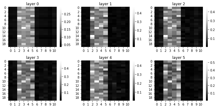
(b) Masks of Trompt.

Figure 19: Attention masks of each layer on Syn2 dataset.

(a) Important Features.

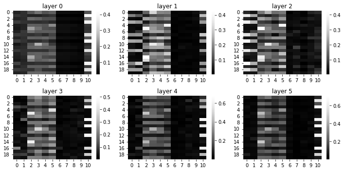
(b) Masks of Trompt.

Figure 20: Attention masks of each layer on Syn4 dataset.

E.2 Additional Real-world Datasets

The additional interpretability experiments were conducted on the red wine quality dataset and white wine quality dataset (Cortez et al., 2009). According to the descriptions of dataset, feature selections are required since there are noisy columns in both datasets. The experimental results are presented in Tables 28 and 29. The results indicate that both Trompt and tree-based models yielded comparable feature importances. Specifically, Trompt assigned higher scores to the alcohol and sulphates columns in the red wine quality dataset, and the volatile acidity column in the white wine quality dataset.

Table 28: The top-3 importance score ratio on the red wine quality dataset.

	1st	2nd	3rd
RandomForest	alcohol ($27.17\%$)	sulphates ($15.44\%$)	volatile acidity ($10.92\%$)
XGBoost	alcohol ($35.42\%$)	sulphates ($15.44\%$)	volatile acidity ($7.56\%$)
LightGBM	alcohol ($26.08\%$)	sulphates ($15.75\%$)	volatile acidity ($10.63\%$)
CatBoost	sulphates ($16.29\%$)	alcohol ($15.67\%$)	volatile acidity ($10.40\%$)
GradientBoostingTree	alcohol ($26.27\%$)	sulphates ($16.24\%$)	volatile acidity ($11.12\%$)
Trompt (ours)	alcohol ($11.83\%$)	sulphates ($10.94\%$)	total sulfur dioxide ($9.78\%$)

Table 29: The top-3 importance score ratio on the white wine quality dataset.

	1st	2nd	3rd
RandomForest	alcohol ($24.22\%$)	volatile acidity ($12.44\%$)	free sulfur dioxide ($11.78\%$)
XGBoost	alcohol ($31.87\%$)	free sulfur dioxide ($11.38\%$)	volatile acidity ($10.05\%$)
LightGBM	alcohol ($24.02\%$)	volatile acidity ($12.47\%$)	free sulfur dioxide ($11.45\%$)
CatBoost	alcohol ($17.34\%$)	volatile acidity ($12.07\%$)	free sulfur dioxide ($11.47\%$)
GradientBoostingTree	alcohol ($27.84\%$)	volatile acidity ($13.59\%$)	free sulfur dioxide ($12.87\%$)
Trompt (ours)	fixed acidity ($10.91\%$)	volatile acidity ($10.47\%$)	pH ($10.37\%$)

Appendix F Hyperparameter Search Spaces

The hyperparameter search space of all models is defined in Tables 30, 31, 32, 33, 34, 35, 36, 37, 38 and 39. We use the same search spaces for the models tested in Grinsztajn45 and additionally define the search spaces for CatBoost, LightGBM, and Trompt since they are newly added. For CatBoost, we followed the search spaces declared by FT-Transformer (Gorishniy et al., 2021). For LightGBM, we followed the search spaces suggested by practitioners (Averagemn, 2019; Bahmani, 2022).

Notice that for the hyperparameter search space of Trompt, we focus on the variation of deriving feature importances (part one of Figure 3). In the default design, we apply concatenation on $\mathbf{SE}_{\text{prompt}}$ and $\mathbf{O}_{\text{prev}}$. Here, we explore the possibility of summation. Additionally, if we applied summation, the following dense layer is not necessary. Here, we explore the possibility of removing the dense layer. As for dense, we explore the variation of sharing weight among all prompts. Lastly, removing residual connections of Equation Equation 2 is also explored. Besides the variation of deriving feature importances, we also explore removing the residual connection of expanding feature embeddings (part three of Figure 3). In addition, we adjust the minimal batch ratio so that Trompt can be trained using different batch sizes.

To clarify, since the dense layer must be applied if concatenation was applied, and sharing dense must be false if the dense layer was not applied, the effective parameter combinations of Table 30 amount to 40.

Table 30: Hyperparameter space of Trompt.

Parameter	Distribution
Feature Importances Type	$[\mathtt{concat},\mathtt{add}]$
Feature Importances Dense	$[\mathtt{true},\mathtt{false}]$
Feature Importances Residual Connection	$[\mathtt{true},\mathtt{false}]$
Feature Importances Sharing Dense	$[\mathtt{true},\mathtt{false}]$
Feature Embeddings Residual Connection	$[\mathtt{true},\mathtt{false}]$
Minimal Batch Ratio	$[0.1,0.01]$

Table 31: Hyperparameter space of FT-Transformer.

Parameter	Distribution
Num Layers	$\mathtt{uniform\_int}[1,6]$
Feature Embedding Size	$\mathtt{uniform\_int}[64,512]$
Residual Dropout	$\mathtt{uniform}[0,0.5]$
Attention Dropout	$\mathtt{uniform}[0,0.5]$
FFN Dropout	$\mathtt{uniform}[0,0.5]$
FFN Factor	$\mathtt{uniform}[2/3,8/3]$
Learning Rate	$\mathtt{log\_uniform}[1e-5,1e-3]$
Weight Decay	$\mathtt{log\_uniform}[1e-6,1e-3]$
KV Compression	$[\mathtt{true},\mathtt{false}]$
LKV Compression Sharing	$[\mathtt{headwise},\mathtt{key\_value}]$
Learning Rate Scheduler	$[\mathtt{true},\mathtt{false}]$
Batch Size	$[256,512,1024]$

Table 32: Hyperparameter space of ResNet.

Parameter	Distribution
Num Layers	$\mathtt{uniform\_int}[1,16]$
Layers Size	$\mathtt{uniform\_int}[64,1024]$
Hidden Factor	$\mathtt{uniform}[1,4]$
Hidden Dropout	$[0,0.5]$
Residual Dropout	$\mathtt{uniform}[0,0.5]$
Learning Rate	$\mathtt{log\_uniform}[1e-5,1e-2]$
Weight Decay	$\mathtt{log\_uniform}[1e-8,1e-3]$
Category Embedding Size	$\mathtt{uniform\_int}[64,512]$
Normalization	$[\mathtt{batch\_norm},\mathtt{layer\_norm}]$
Learning Rate Scheduler	$[\mathtt{true},\mathtt{false}]$
Batch Size	$[256,512,1024]$

Table 33: Hyperparameter space of MLP.

Parameter	Distribution
Num Layers	$\mathtt{uniform\_int}[1,8]$
Layer Size	$\mathtt{uniform\_int}[16,1024]$
Dropout	$[0,0.5]$
Learning Rate	$\mathtt{log\_uniform}[1e-5,1e-2]$
Category Embedding Size	$\mathtt{uniform\_int}[64,512]$
Learning Rate Scheduler	$[\mathtt{true},\mathtt{false}]$
Batch Size	$[256,512,1024]$

Table 34: Hyperparameter space of SAINT.

Parameter	Distribution
Num Layers	$\mathtt{uniform\_int}[1,2,3,6,12]$
Num Heads	$[2,4,8]$
Layer Size	$\mathtt{uniform\_int}[32,64,128]$
Dropout	$[0,0.1,0.2,0.3,0.4,0.5,0.6,0.7,0.8]$
Learning Rate	$\mathtt{log\_uniform}[1e-5,1e-3]$
Batch Size	$[128,256]$

Table 35: Hyperparameter space of CatBoost.

Parameter	Distribution
Max Depth	$[3,4,5,6,7,8,9,10]$
Learning Rate	$\mathtt{log\_uniform}[1e-5,1]$
Iterations	$\mathtt{quantile\_uniform}[100,6000]$
Bagging Temperature	$\mathtt{uniform}[0,1]$
L2 Leaf Reg	$\mathtt{log\_uniform}[1,10]$
Leaf Estimation Iteration	$[1,2,3,4,5,6,7,8,9,10]$

Table 36: Hyperparameter space of LightGBM.

Parameter	Distribution
Learning Rate	$\mathtt{uniform}[0.001,1]$
Max Depth	$[1,2,3,4,5,6,7,8,9,10,11]$
Bagging Fraction	$\mathtt{uniform}[0.1,1.0]$
Bagging Frequency	$[1,2,3,4,5]$
Num Leaves	$\mathtt{quantile\_uniform}[30,150]$
Feature Fraction	$\mathtt{uniform}[0.1,1.0]$
Num Estimators	$1000$
Boosting	$[\mathtt{gbdt},\mathtt{rf},\mathtt{dart}]$

Table 37: Hyperparameter space of XGBoost.

Parameter	Distribution
Max Depth	$\mathtt{uniform\_int}[1,11]$
Num Estimators	$1000$
Min Child Weight	$\mathtt{log\_uniform\_int}[1,1e2]$
Subsample	$\mathtt{unifrom}[0.5,1]$
Learning Rate	$\mathtt{log\_unifrom}[1e-5,0.7]$
Col Sample by Level	$\mathtt{uniform}[0.5,1]$
Col Sample by Tree	$\mathtt{uniform}[0.5,1]$
Gamma	$\mathtt{log\_uniform}[1e-8,7]$
Lambda	$\mathtt{log\_uniform}[1,4]$
Alpha	$\mathtt{log\_uniform}[1e-8,1e2]$

Table 38: Hyperparameter space of RandomForest.

Parameter	Distribution
Max Depth	$[\mathtt{none},2,3,4]([0.7,0.1,0.1,0.1])$
Num Estimators	$250$
Criterion	$[\mathtt{gini},\mathtt{entropy}]([\mathtt{squared\_error},\mathtt{absolute\_error}])$
Max Features	$[\mathtt{sqrt},\mathtt{log2},\mathtt{none},0.1,0.2,0.3,0.4,0.5,0.6,0.7,0.8,0.9]$
Min Samples Split	$[2,3]([0.95,0.05])$
Min Samples Leaf	$\mathtt{log\_uniform\_int}[1.5,50.5]$
Bootstrap	$[\mathtt{true},\mathtt{false}]$
Min Impurity Decrease	$[0.0,0.01,0.02,0.05]([0.85,0.05,0.05,0.05])$

Table 39: Hyperparameter space of GradientBoostingTree.

Parameter	Distribution
Loss	$[\mathtt{deviance},\mathtt{exponential}](classif)([\mathtt{squared\_error},\mathtt{absolute\_error},\mathtt{huber}])(regression)$
Learning Rate	$\mathtt{log\_normal}[\mathtt{log}(0.01),\mathtt{log}(10)]$
Subsample	$\mathtt{uniform}[0.5,1]$
Num Estimators	$1000$
Criterion	$[\mathtt{friedman\_mse},\mathtt{squared\_error}]$
Max Depth	$[\mathtt{none},2,3,4,5]([0.1,0.1,0.5,0.1,0.1])$
Min Samples Split	$[2.3]([0.95,0.05])$
Min Impurity Decrease	$[0.0,0.01,0.02,0.05]([0.85,0.05])$
Max Leaf Nodes	$[\mathtt{none},5,10,15]([0.85,0.5])$

Table 40: Hyperparameter space of HistGradientBoosting.

Parameter	Distribution
Loss	$[\mathtt{squared\_error},\mathtt{absolute\_error},\mathtt{huber}](regression)$
Learning Rate	$\mathtt{log\_normal}[\mathtt{log}(0.01),\mathtt{log}(10)]$
Max Iteration	$1000$
Min Depth	$[\mathtt{none},2,3,4]$
Min Samples Leaf	$\mathtt{normal\_int}[20,2]$
Max Leaf Nodes	$\mathtt{normal\_int}[31,5]$

References

- Arik & Pfister (2021) Arik, S. Ö. and Pfister, T. Tabnet: Attentive interpretable tabular learning. In Proceedings of the AAAI Conference on Artificial Intelligence, volume 35, pp. 6679–6687, 2021.
- Averagemn (2019) Averagemn. Lgbm with hyperopt tuning, 2019. URL https://www.kaggle.com/code/donkeys/lgbm-with-hyperopt-tuning/notebook. [Online; accessed 5-January-2023].
- Bahmani (2022) Bahmani, M. Understanding lightgbm parameters (and how to tune them), 2022. URL https://neptune.ai/blog/lightgbm-parameters-guide. [Online; accessed 5-January-2023].
- Borisov et al. (2021) Borisov, V., Leemann, T., Seßler, K., Haug, J., Pawelczyk, M., and Kasneci, G. Deep neural networks and tabular data: A survey. arXiv preprint arXiv:2110.01889, 2021.
- Breiman (2001) Breiman, L. Random forests. Machine learning, 45(1):5–32, 2001.
- Brown et al. (2020) Brown, T., Mann, B., Ryder, N., Subbiah, M., Kaplan, J. D., Dhariwal, P., Neelakantan, A., Shyam, P., Sastry, G., Askell, A., et al. Language models are few-shot learners. Advances in neural information processing systems, 33:1877–1901, 2020.
- Chen et al. (2018) Chen, J., Song, L., Wainwright, M., and Jordan, M. Learning to explain: An information-theoretic perspective on model interpretation. In International Conference on Machine Learning, pp. 883–892. PMLR, 2018.
- Chen et al. (2021) Chen, L., Lu, K., Rajeswaran, A., Lee, K., Grover, A., Laskin, M., Abbeel, P., Srinivas, A., and Mordatch, I. Decision transformer: Reinforcement learning via sequence modeling. Advances in neural information processing systems, 34:15084–15097, 2021.
- Chen et al. (2015) Chen, T., He, T., Benesty, M., Khotilovich, V., Tang, Y., Cho, H., Chen, K., et al. Xgboost: extreme gradient boosting. R package version 0.4-2, 1(4):1–4, 2015.
- Cortez et al. (2009) Cortez, P., Cerdeira, A., Almeida, F., Matos, T., and Reis, J. Modeling wine preferences by data mining from physicochemical properties. Decision support systems, 47(4):547–553, 2009.
- Devlin et al. (2018) Devlin, J., Chang, M.-W., Lee, K., and Toutanova, K. Bert: Pre-training of deep bidirectional transformers for language understanding. arXiv preprint arXiv:1810.04805, 2018.
- Dosovitskiy et al. (2020) Dosovitskiy, A., Beyer, L., Kolesnikov, A., Weissenborn, D., Zhai, X., Unterthiner, T., Dehghani, M., Minderer, M., Heigold, G., Gelly, S., et al. An image is worth 16x16 words: Transformers for image recognition at scale. arXiv preprint arXiv:2010.11929, 2020.
- Dua & Graff (2017) Dua, D. and Graff, C. UCI machine learning repository, 2017. URL http://archive.ics.uci.edu/ml.
- Friedman (2001) Friedman, J. H. Greedy function approximation: a gradient boosting machine. Annals of statistics, pp. 1189–1232, 2001.
- Goodfellow et al. (2020) Goodfellow, I., Pouget-Abadie, J., Mirza, M., Xu, B., Warde-Farley, D., Ozair, S., Courville, A., and Bengio, Y. Generative adversarial networks. Communications of the ACM, 63(11):139–144, 2020.
- Gorishniy et al. (2021) Gorishniy, Y., Rubachev, I., Khrulkov, V., and Babenko, A. Revisiting deep learning models for tabular data. Advances in Neural Information Processing Systems, 34:18932–18943, 2021.
- Grinsztajn et al. (2022) Grinsztajn, L., Oyallon, E., and Varoquaux, G. Why do tree-based models still outperform deep learning on typical tabular data? In Thirty-sixth Conference on Neural Information Processing Systems Datasets and Benchmarks Track, 2022. URL https://openreview.net/forum?id=Fp7__phQszn.
- Gu et al. (2017) Gu, S., Holly, E., Lillicrap, T., and Levine, S. Deep reinforcement learning for robotic manipulation with asynchronous off-policy updates. In 2017 IEEE international conference on robotics and automation (ICRA), pp. 3389–3396. IEEE, 2017.
- He et al. (2016) He, K., Zhang, X., Ren, S., and Sun, J. Deep residual learning for image recognition. In Proceedings of the IEEE conference on computer vision and pattern recognition, pp. 770–778, 2016.
- Huang et al. (2020) Huang, X., Khetan, A., Cvitkovic, M., and Karnin, Z. Tabtransformer: Tabular data modeling using contextual embeddings. arXiv preprint arXiv:2012.06678, 2020.
- Katzir et al. (2020) Katzir, L., Elidan, G., and El-Yaniv, R. Net-dnf: Effective deep modeling of tabular data. In International Conference on Learning Representations, 2020.
- Ke et al. (2017) Ke, G., Meng, Q., Finley, T., Wang, T., Chen, W., Ma, W., Ye, Q., and Liu, T.-Y. Lightgbm: A highly efficient gradient boosting decision tree. Advances in neural information processing systems, 30, 2017.
- LeCun et al. (1995) LeCun, Y., Bengio, Y., et al. Convolutional networks for images, speech, and time series. The handbook of brain theory and neural networks, 3361(10):1995, 1995.
- LeCun et al. (2015) LeCun, Y., Bengio, Y., and Hinton, G. Deep learning. nature, 521(7553):436–444, 2015.
- Lester et al. (2021) Lester, B., Al-Rfou, R., and Constant, N. The power of scale for parameter-efficient prompt tuning. arXiv preprint arXiv:2104.08691, 2021.
- Li & Liang (2021) Li, X. L. and Liang, P. Prefix-tuning: Optimizing continuous prompts for generation. arXiv preprint arXiv:2101.00190, 2021.
- Prokhorenkova et al. (2018) Prokhorenkova, L., Gusev, G., Vorobev, A., Dorogush, A. V., and Gulin, A. Catboost: unbiased boosting with categorical features. Advances in neural information processing systems, 31, 2018.
- Radford et al. (2018) Radford, A., Narasimhan, K., Salimans, T., Sutskever, I., et al. Improving language understanding by generative pre-training. 2018.
- Ramachandram & Taylor (2017) Ramachandram, D. and Taylor, G. W. Deep multimodal learning: A survey on recent advances and trends. IEEE signal processing magazine, 34(6):96–108, 2017.
- Redmon et al. (2016) Redmon, J., Divvala, S., Girshick, R., and Farhadi, A. You only look once: Unified, real-time object detection. In Proceedings of the IEEE conference on computer vision and pattern recognition, pp. 779–788, 2016.
- Rumelhart et al. (1986) Rumelhart, D. E., Hinton, G. E., and Williams, R. J. Learning representations by back-propagating errors. nature, 323(6088):533–536, 1986.
- Sahoo et al. (2017) Sahoo, D., Pham, Q., Lu, J., and Hoi, S. C. Online deep learning: Learning deep neural networks on the fly. arXiv preprint arXiv:1711.03705, 2017.
- scikit learn (2023a) scikit learn. sklearn.ensemble.histgradientboostingclassifier, 2023a. URL https://scikit-learn.org/stable/modules/generated/sklearn.ensemble.HistGradientBoostingClassifier.html. [Online; accessed 21-January-2023].
- scikit learn (2023b) scikit learn. sklearn.preprocessing.quantiletransformer, 2023b. URL https://scikit-learn.org/stable/modules/generated/sklearn.preprocessing.QuantileTransformer.html. [Online; accessed 26-January-2023].
- Shwartz-Ziv & Armon (2022) Shwartz-Ziv, R. and Armon, A. Tabular data: Deep learning is not all you need. Information Fusion, 81:84–90, 2022. ISSN 1566-2535. doi: https://doi.org/10.1016/j.inffus.2021.11.011. URL https://www.sciencedirect.com/science/article/pii/S1566253521002360.
- Somepalli et al. (2021) Somepalli, G., Goldblum, M., Schwarzschild, A., Bruss, C. B., and Goldstein, T. Saint: Improved neural networks for tabular data via row attention and contrastive pre-training. arXiv preprint arXiv:2106.01342, 2021.
- Van Engelen & Hoos (2020) Van Engelen, J. E. and Hoos, H. H. A survey on semi-supervised learning. Machine Learning, 109(2):373–440, 2020.
- Vanschoren et al. (2013) Vanschoren, J., van Rijn, J. N., Bischl, B., and Torgo, L. Openml: networked science in machine learning. SIGKDD Explorations, 15(2):49–60, 2013. doi: 10.1145/2641190.2641198. URL http://doi.acm.org/10.1145/2641190.264119.
- Vaswani et al. (2017) Vaswani, A., Shazeer, N., Parmar, N., Uszkoreit, J., Jones, L., Gomez, A. N., Kaiser, Ł., and Polosukhin, I. Attention is all you need. Advances in neural information processing systems, 30, 2017.
- Zhang et al. (2020) Zhang, Q., Lu, H., Sak, H., Tripathi, A., McDermott, E., Koo, S., and Kumar, S. Transformer transducer: A streamable speech recognition model with transformer encoders and rnn-t loss. In ICASSP 2020-2020 IEEE International Conference on Acoustics, Speech and Signal Processing (ICASSP), pp. 7829–7833. IEEE, 2020.