Are We There Yet? Product Quantization and its Hardware Acceleration

Abstract

Conventional multiply-accumulate (MAC) operations have long dominated computation time for deep neural networks (DNNs). Recently, product quantization (PQ) has been successfully applied to these workloads, replacing MACs with memory lookups to pre-computed dot products. While this property makes PQ an attractive solution for model acceleration, little is understood about the associated trade-offs in terms of compute and memory footprint, and the impact on accuracy. Our empirical study investigates the impact of different PQ settings and training methods on layerwise reconstruction error and end-to-end model accuracy. When studying the efficiency of deploying PQ DNNs, we find that metrics such as FLOPs, number of parameters, and even CPU/GPU performance, can be misleading. To address this issue, and to more fairly assess PQ in terms of hardware efficiency, we design the first custom hardware accelerator to evaluate the speed and efficiency of running PQ models. We identify PQ configurations that are able to improve performance-per-area for ResNet20 by 40%–104%, even when compared to a highly optimized conventional DNN accelerator. Our hardware performance outperforms recent PQ solutions by 4x, with only a 0.6% accuracy degradation. This work demonstrates the practical and hardware-aware design of PQ models, paving the way for wider adoption of this emerging DNN approximation methodology.

1 Introduction

Model optimisation has taken many forms, including pruning [6], quantization [47, 27, 58], lightweight architectural designs [48, 52, 42], and faster algorithms [38, 54, 9, 18]. Each of these techniques offers different trade-offs in terms of inference acceleration, model compression, hardware acceleration suitability, and accuracy degradation. Some methods focus solely on decreasing the number or computations while not affecting model size (e.g. Winograd [38]). Other methods such as linear quantization and pruning tend to generally decrease both computation and memory footprint. While other methods such as some forms of non-linear quantization [49] only decrease model size, and leave the number of computations unaffected. On this spectrum of compute and memory tradeoffs, a new compression methodology, product quantization (PQ), sits on one extreme. Specifically, PQ can eliminate all multiplications from a matrix multiplication operation [7], making it an interesting new compression method worth further investigation. Our work thoroughly investigates this emerging compression methodology and determines its practicality and hardware acceleration potential.

Approximate nearest neighbours for information retrieval involves extracting a compact representation of high-dimensional features, for example images [61, 30], in order to fetch similar ones from a data source. One method to encode these input features is PQ [34]. Recently, it has been repurposed for model inference acceleration [7] by encoding layer inputs into a set of learnable prototypes. With the index resulting from this mapping, the pre-computed dot product between inputs and the corresponding layer parameters is retrieving from a lookup table. However, the existing works offer a limited evaluation of PQ either by exclusively applying it to the final layer of the model [7], extremely simple networks [40], or by not taking into account the overheads associated with this optimization. This is the case in the recently-published PECAN [45], which uses short codes to lessen the degradation that PQ introduces at the cost of 20$\times$ larger model memory footprint.

Motivated by the potential of PQ for inference acceleration, we: (1) provide a systematic study on the parameterisation and training of PQ and its impact on compute and memory footprint as well as encoding degradation; (2) present the first hardware accelerator for lightweight PQ CNNs, demonstrating that unlike GPUs and CPUs, custom hardware can indeed accelerate PQ; and (3) evaluate PQ comprehensively for three CNNs and we identify configurations that achieve 4–6$\times$ higher hardware performance compared to recent PQ literature. Unlike other DNN compression methods, e.g. quantization or pruning, PQ is new technique that is poorly understood, especially when it comes to its hardware efficiency potential. Our work substantially bridges the gap between the accuracy of PQ DNNs and their intrinsic hardware performance, through a comprehensive accuracy/efficiency study of PQ configurations using a custom-built, hardware PQ accelerator.

2 Related Work

Quantization. A multitude of methods have been proposed to quantize models from FP32 to lower bitwidths [27, 57, 44, 20, 51] each offering different trade offs in terms of model compression, inference speedup and degradation. From its many instantiations, INT8 quantization has attracted the most attention due to its support on off-the-shelve devices [39, 17, 50, 28, 56], and lower chip area and energy requirements when designing custom hardware [26, 60].

Product Quantization. Standard quantization approaches perform a scalar-to-scalar mapping while product quantization (PQ) operates with higher-dimensional elements mapping vectors to vectors [34, 19]. This has made PQ a good fit for applications such as image retrieval [61, 36, 30] and compression [49, 14]. Different from those works is [7], where PQ is used to accelerate matrix-matrix multiplications in a two-step process: columns of the input are mapped to prototypes, a set of learnable vectors; then these vectors are used to construct a look-up table of pre-computed dot products between prototypes and the layer weights. At inference time, the pre-computed values can be retrieved by mapping each input column to its closest prototype, trading numerical degradation for larger speedups in some cases. Follow up work extends PQ to an entire fully connected network and provides a preliminary analysis on the overheads of accelerating PQ [40]. A more generalised implementation of PQ is PECAN [45], which not only applies PQ to CNNs but also proposes a distance metric for input-to-prototype encoding that does not require multiplications. However, their implementation resulted in severe memory overheads that were not carefully considered as the objective of getting rid of multiplications and minimising accuracy degradation was prioritised. Unlike prior work, we perform a broader and systematic study of the impact of PQ settings in terms of memory, compute, and accuracy which we then use to inform our hardware accelerator design.

Hardware Acceleration of DNNs. Many custom hardware accelerators have been developed, especially for DNNs. These accelerators outperform conventional CPUs and GPUs by leveraging DNN-specific properties in their hardware architectures [15, 10, 16]. For example, Google’s TPU [33] uses a 2D systolic array of multiply-accumulate units that can more directly and efficiently transfer data between compute units instead of expensive synchronization over GPU register files. Another example is Groq’s TSP [2], which utilizes spatial compute units to enable the construction of custom compute engines for each DNN layer. Many prior works have used field-programmable gate-arrays (FPGAs) to build accelerators for deep learning, leveraging low precision, sparsity, a custom memory hierarchy, or novel dataflows [3, 1, 22]. However, none of the existing work has attempted to accelerate PQ using custom hardware, nor were there any studies of PQ efficiency using a custom accelerator. Our work aims to fill this gap by presenting the first product quantization accelerator.

Product Quantization is a big departure from previous methods (e.g. pruning, quantization, sparsity) for model acceleration. Because of this, a new training protocol is needed which captures the encoding+lookup stages of PQ (more in Sec. 3). Furthermore, a radically new hardware design is required in order to accurately quantify the efficiency potential of PQ (see Sec. 5). These characteristics make PQ a challenging method to implement and therefore motivates our study and contributions.

3 Background

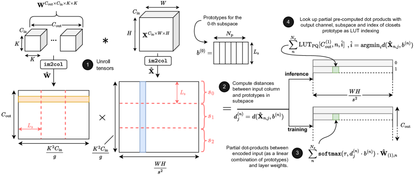
Figure 1: Transforming a convolutional layer into its PQ equivalent. First, both input and weights tensors need to be unrolled, resulting in $\mathbf{\hat{X}}$ and $\mathbf{\hat{W}}$. The input matrix $\mathbf{\hat{X}}$ is subdivided into $N_{s}$ subspaces (three in this diagram), and the sub-columns in each one will be encoded using their respective bank of of prototypes $\mathbf{B}_{l}\!=\![\mathbf{b}^{(0)},\mathbf{b}^{(1)},\mathbf{b}^{(2)}]$. Given a distance metric $d(\cdot)$, e.g. Euclidean distance, the input is encoded in a soft manner during training but replaced with a hard one-hot encoding during inference. For deployment, the layer weights $\mathbf{W}$ are not needed, since all the pre-computed dot products are stored in table $\text{LUT}_{\text{PQ}}$.

Accelerating inference with Product Quantization requires introducing changes in the way models are trained. This section starts by introducing the process of converting standard linear or convolutional layers into PQ layers. Then we present the method followed to train such layers and highlight the challenges and overheads that this aggressive quantization formulation introduces.

3.1 Deriving Product-Quantizable Layers

Almost all layers found in modern ML architectures that transform an input $\mathbf{X}$ into an output $\mathbf{Y}$ using parameters $\mathbf{W}$, including those in CNNs [23, 48, 52, 4] or transformers [55, 13, 41], can be expressed as a matrix-matrix multiplication. This is evident for standard fully connected layers where an input $\mathbf{X}\!\in\!\mathcal{R}^{A\times C_{\text{in}}}$ is transformed by weights $\mathbf{W}\!\in\!\mathcal{R}^{C_{\text{out}}\times A}$ to obtain output $\mathbf{Y}\!\in\!\mathcal{R}^{A\times C_{\text{out}}}$, where $C_{\text{in}}$ and $C_{\text{out}}$ are the number of input and output features or, more generically, channels. In the case of convolutions, both input $\mathbf{X}\!\in\!\mathcal{R}^{C_{\text{in}}\times W\times H}$ and weights $\mathbf{W}\!\in\!\mathcal{R}^{C_{\text{out}}\times C_{\text{in}}\times K_{\text{w}}\times K_{\text{h}}}$ tensors first need to be unrolled. This unrolling can be done following the im2col algorithm [32, 21], resulting in unrolled matrices of size $(K_{w}K_{h}C_{\text{in}}/g)\times(WH/s^{2})$ and $C_{\text{out}}\times(K_{\text{w}}K_{\text{h}}C_{\text{in}}/g)$ for input and weights tensors respectively with $s$ and $g$ representing stride and groups respectively.

We now introduce PQ-specific terms and assume a matrix of weights $\mathbf{W}\!\in\!\mathcal{R}^{C_{\text{out}}\times A}$ and of inputs $\mathbf{X}\!\in\!\mathcal{R}^{A\times C_{\text{in}}}$ exist, whether they are from a linear layer or are the result of a tensor unrolling. With PQ, we aim to aggressively quantise the input matrix on-the-fly so that the multiplication with $\mathbf{W}$ can be reduced to a series of lookups to a table of pre-computed dot-products of size $\text{LUT}_{\text{PQ}}\!\in\!\mathcal{R}^{C_{\text{out}}\times N_{\text{s}}\times N_{\text{p}}}$. The input $\mathbf{X}$ can be split into $N_{\text{s}}$ disjoint groups along the rows dimension. We call each of these groups subspaces. See Fig 1. Each subspace gets assigned a bank of prototypes $\mathbf{b}^{(n)}$ of size $L_{\text{s}}\times N_{\text{p}}$, where $N_{\text{p}}$ and $L_{\text{s}}$ represent the number and the length of the prototypes. This list of prototypes banks $\mathbf{B}_{l}\!=\![\mathbf{b}^{(0)},\mathbf{b}^{(1)},...,\mathbf{b}^{(N_{\text{s}}-1)}]$ are learnable parameters of PQ layers, with subscript $l$ denoting the layer index. PQ involves getting the index of the closest prototype via distance $d(\cdot)$ to each sub-column of the input matrix (i.e. vectors of length $L_{\text{s}}$). As a result, and as it will become apparent later in Sec 4, there is a trade-off between $N_{\text{p}}$ and $N_{\text{s}}$, both impacting the encoding error introduced, the compute overheads of $d(\cdot)$, and the memory footprint of table $\text{LUT}_{\text{PQ}}$.

3.2 Training and Deploying PQ Models

Training PQ layers involves learning two sets of parameters: the standard layer weights $\mathbf{W}_{l}$ and prototypes $\mathbf{B}_{l}$. Then, prior to deployment, the table of pre-computed dot products $\text{LUT}_{\text{PQ}}$ is obtained by performing a Cartesian product between $\mathbf{W}_{l}$ and $\mathbf{B}_{l}$. Only $\text{LUT}_{\text{PQ}}$ and $\mathbf{B}_{l}$ are deployed.

Choosing a distance metric. For both training and inference, a distance $d(\cdot)$ needs to be defined to encode the input using the layer prototypes $\mathbf{B}_{l}$. A reasonable choice would be the Euclidean distance. For PQ, the relative ranking of distances between input column $\mathbf{\hat{X}}_{n,j}$ and the prototypes of that subspace $\mathbf{b}^{(n)}$ is far more important than the actual distance value. This therefore leaves room for more lightweight distance metrics such as the $L_{1}$ Manhattan distance.

Input encoding. During training the encoding of the input is done explicitly, i.e., the unrolled input $\mathbf{\hat{X}}$ is actually transformed into a new matrix of the same dimensions that is later multiplied with the unrolled layer weights $\mathbf{\hat{W}}$. Given the $j$-th column of $\mathbf{\hat{X}}$ along the $n$-th subspace, $\mathbf{\hat{X}}_{n,j}$, the distances $\mathbf{d}^{(n)}_{j}=d(\mathbf{\hat{X}}_{n,j},\mathbf{b}^{(n)})$ to each of the prototypes are computed. The encoded portion of the input $\mathbf{\hat{X}^{\text{enc}}}_{n,j}$ is obtained by a weighed linear combination of $\mathbf{b}^{(n)}$ with normalised distances $\phi(\tau,\mathbf{d}^{(n)}_{j})$

$$\mathbf{\hat{X}^{\text{enc}}}_{n,j}=\phi\left(\tau,\mathbf{d}^{(n)}_{j}\right)\mathbf{b}^{(n)}=\sum^{N_{\text{p}}}_{p}\frac{\mathbf{b}^{\text{(n)}}_{p}\text{exp}(d^{(n,p)}_{j}/\tau)}{\sum^{N_{\text{p}}}_{k}\text{exp}(d^{(n,k)}_{j}/\tau)}$$ (1)

where $\mathbf{b}^{\text{(n)}}_{p}$ stands for the $p$-th prototype in the $n$-th subspace, $d^{(n,p)}_{j}$ is the distance to the p-th prototype, and $\tau$ is a temperature factor. As $\tau\rightarrow 0$, the temperatured-softmax $\phi(\tau,\cdot)$ outputs a sharper distribution over $\mathbf{d}^{(n)}_{j}$, transitioning in this way from soft linear combination of prototypes into a hard, one-hot encoding. During inference PQ is implemented with one-hot assignments.

Constructing $\text{LUT}_{\text{PQ}}$. During inference, $\mathbf{\hat{X}^{\text{enc}}}_{n,j}$ is not materialised since only the index of the closest prototype is needed to retrieve the partial dot product from $\text{LUT}_{\text{PQ}}$. Once training has ended, the unrolled weights $\mathbf{\hat{W}}$ can be partitioned into subspaces along the column dimension (as shown in Fig 1). Then, the dot product between a $1\times L_{\text{s}}$ sub-row in $\mathbf{\hat{W}}$ and a prototype in such subspace, corresponds to one entry in $\text{LUT}_{\text{PQ}}$. Repeating this for all $N_{s}$, $C_{\text{out}}$ and $N_{\text{p}}$ completes the table.

3.3 PQ Implementation Trade-Offs

Different parameterizations of PQ (i.e. choice of {$N_{\text{p}}$,$N_{\text{s}}$}), will lead to dramatically different levels of model acceleration, memory footprint, and degradation. Understanding these trade-offs is fundamental to the design of PQ models.

Compute footprint. The number of FLOPs to perform an im2col-equivalent convolution (as in Fig 1) is given by $\text{FLOPs}_{\tt{im2col}}\!=\!2K^{2}C_{\text{in}}WHC_{\text{out}}$, assuming groups and stride equal to one and squared kernels. The same layer but implemented with PQ would result in $\text{FLOPs}_{\text{PQ}}\!=\!\text{FLOPs}^{\text{enc}}\!+\!\text{FLOPs}^{\text{add}}\!$. The first term is given by $\text{FLOPs}^{\text{enc}}\!=\!N_{\text{s}}d(\cdot)_{\text{FLOPs}}WH$, with $d(\cdot)_{\text{FLOPs}}$ representing the FLOPs to compute the distances $\mathbf{d}^{(n)}_{j}$. Assuming Euclidean distance, $d(\cdot)_{\text{FLOPs}}\!=\!3N_{\text{p}}L_{\text{s}}$. Term $\text{FLOPs}^{\text{add}}\!=\!(N_{\text{s}}-1)WHC_{\text{out}}$ accounts for the cost of performing the addition of partial dot-products needed to complete a full row-column dot-product $\mathbf{\hat{X}}\!\cdot\!\mathbf{\hat{W}}$. The FLOPs savings ratio is given by

$$\frac{\text{FLOPs}_{\tt{im2col}}}{\text{FLOPs}_{\text{PQ}}}=\frac{2K^{2}C_{\text{in}}WHC_{\text{out}}}{N_{\text{s}}WH(\text{FLOPs}^{\text{enc}}+C_{\text{out}})}=\frac{2C_{\text{out}}L_{\text{s}}}{\text{FLOPs}^{\text{enc}}+C_{\text{out}}}=\frac{2C_{\text{out}}L_{\text{s}}}{3N_{\text{p}}L_{\text{s}}+C_{\text{out}}}$$ (2)

with $N_{\text{s}}\!=\!K^{2}C_{\text{in}}/L_{\text{s}}$ and simplifying $(N_{\text{s}}\!-\!1)$ as just $N_{\text{s}}$. This expression suggest that reducing the number of prototypes has a larger impact than increasing their length. See App. D for numerical results.

Memory footprint. The number of parameters in a convolutional layer is given by $C_{\text{out}}C_{\text{in}}K^{2}$, assuming squared kernels and groups=1. When transformed into PQ, this number becomes $\text{params}_{\text{PQ}}\!=\!|\mathbf{B}_{l}|\!+\!|\text{LUT}_{\text{PQ}}|\!=\!N_{\text{s}}N_{\text{p}}(L_{\text{s}}\!+\!C_{\text{out}})$. In this way, and assuming that $C_{\text{out}}\!\gg\!L_{\text{s}}$, savings in parameter count is possible when $C_{\text{in}}K^{2}/N_{\text{s}}N_{\text{p}}\!=\!L_{\text{s}}/{N_{\text{p}}}\!>\!1$, i.e., as it was the case when assessing the compute footprint of PQ, longer prototypes and few of them are also preferred.

Table 1: The best performing models in PECAN-D [45] require a high number of prototypes ($N_{\text{p}}$) of short length ($L_{\text{s}}$). This resulted in look-up tables to be many times larger than the original non-PQ model.

Model	Params	Num. Prototypes ($\text{N}_{\text{p}}$)	Length of Prototypes ($\text{L}_{\text{s}}$)	Size of $\text{LUT}_{\text{PQ}}$	Memory Footprint
LetNet	61K	64	9 & 8	489K	8.0$\times$
ResNet20	269K	128 & 64	3 & 4	5.7M	21.3$\times$

Model degradation. Previous attempts of applying PQ to the entire network required using a larger number of short prototypes to maximise model accuracy. In PECAN-D [45], this translated into a very large increase in memory footprint, see Tab. 1. While intuitively lower $L_{\text{s}}$ should always be preferred when prioritising model degradation, it is unclear what the underlying trade-offs between $N_{\text{p}}$ and $L_{\text{s}}$ are at different layers of a network.

4 Product-Quantizability: Study & Trade-offs

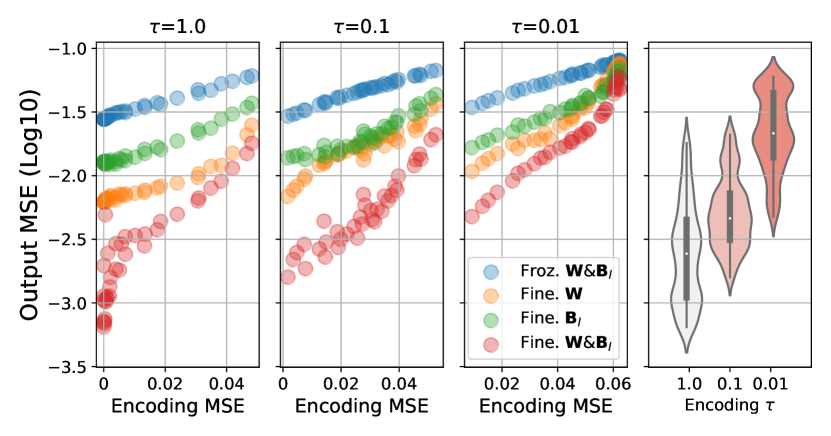
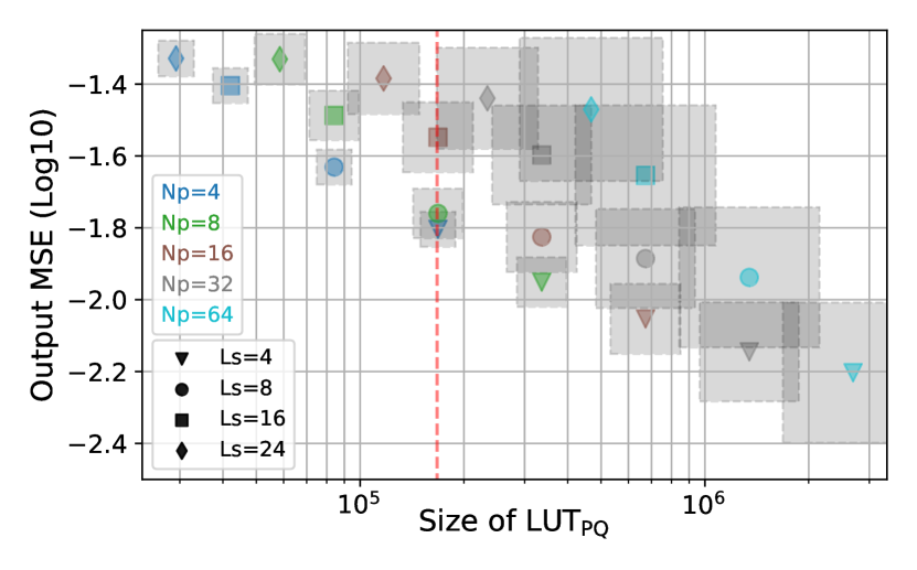
Figure 2: (left) As the temperature $\tau$ decreases, the error in the output of a PQ layer increases rapidly. Even when prototypes and layer parameters are finetuned to minimise MSE($\mathbf{Y}_{\text{PQ}}$,$\mathbf{Y}$), most of the {$N_{\text{p}}$,$L_{\text{s}}$} configurations (each configuration is a dot) leads to much larger error (see top rightmost subplot). (right) Analysis of the 8-th depth-wise layer with $\tau\!=\!0.01$ which receives a $366\!\times\!4\!\times\!4$ input. When spatial dimensions of the input are small relative to their channel dimension, much fewer prototypes (e.g. $N_{\text{p}}\!=\!8$) lead to similar error to other configurations that result in larger $\text{LUT}_{\text{PQ}}$ and a higher $\text{FLOPs}^{\text{enc}}$ (encoding costs, area of grey-shaded squares) as in Eq. 2. The dashed red line indicates the number of parameters in the equivalent non-PQ layer.

In this section we assess the impact of different {$N_{\text{p}}$,$L_{\text{s}}$} in terms of memory and compute footprint as well as accuracy degradation. We design a per-layer analysis where the task for each PQ layer is to generate an output $\mathbf{Y}_{\text{PQ}}$ that is as close as possible to $\mathbf{Y}$, the output of an equivalent layer from a standard, non-PQ, pretrained model. Framing this empirical study in such way enables us to isolate individual layers from the impact of other elements in the model, training hyperparameters, and dynamics. This study uses a CNN containing 10 depth-wise separable convolutional layers designed for image classification on the EMNIST [11] dataset. Implementation details are in App. C.

Given a PQ layer with randomly initialised $\mathbf{B}_{l}$ and weights from its non-PQ counterpart, a two-phases study is conducted. First, the prototypes are trained to minimise $\text{MSE}^{\text{enc}}(\mathbf{\hat{X}^{\text{enc}}},\mathbf{X})$; then, the divergence of $\mathbf{Y}_{\text{PQ}}$ w.r.t. $\mathbf{Y}$ is measured in four different scenarios, namely when every other element in the layer is kept frozen (blue dots in top plot of Fig. 2 (left)), when prototypes are further finetuned to minimise $\text{MSE}^{\text{out}}\!=\!\text{MSE}(\mathbf{Y}_{\text{PQ}},\mathbf{Y})$ (green dots), when only the layer weights are finetuned (orange dots), and when both prototypes and layer weights are jointly finetuned (red dots). All settings involving finetuning start from the same state of trained prototypes (blue dots). These two phases are repeated for a broad {$N_{\text{p}}$, $L_{\text{s}}$, $\tau$} range and across all layers. We make the following observations.

Learning one-hot encodings is hard. As temperature parameter $\tau$ decreases, there is a shift in the distribution over {$N_{\text{p}}$, $L_{\text{s}}$} settings that lead similar $\text{MSE}^{\text{enc}}$ and $\text{MSE}^{\text{out}}$ trends (blue, green orange dots in Fig. 2). More evidently (red dots and violin plot) is the impact on $\text{MSE}^{\text{out}}$ when both layer weights and prototypes are finetuned. These results suggest that at least certain {$N_{\text{p}}$, $L_{\text{s}}$} can perform well at lower $\tau$ values but most cannot.

Reasons for larger $\mathbf{\textit{N}}_{\text{p}}$ decrease with depth. Degradation decreases faster by lowering $L_{\text{s}}$ than increasing $N_{\text{p}}$ as can be observed in Fig. 2 (right). However, this dimension brings a large increase in memory footprint since the size of $\text{LUT}_{\text{PQ}}$ is inversely proportional to $L_{\text{s}}$ (i.e. shorter prototypes lead to more subspaces, which in turn leads to more pre-computed dot products). In comparison, larger $N_{\text{p}}$ has a lesser impact on $\text{MSE}^{\text{out}}$ overall but affects both $\text{LUT}_{\text{PQ}}$ size and $\text{FLOPs}^{\text{enc}}$ linearly. Because of this reason, trading $N_{\text{p}}$ for $L_{\text{s}}$ is desirable even at the cost of some output degradation (e.g. {$N_{\text{p}}\!=\!4$,$L_{\text{s}}\!=\!4$} vs {$N_{\text{p}}\!=\!32$,$L_{\text{s}}\!=\!8$}, the latter resulting in just a $1.13\times$ lower error.).

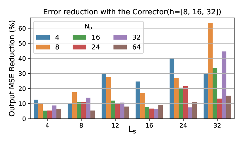
Figure 3: Maximum observed error reduction with corrector: a 2-layer MLP with hidden dimension $h$. For longer and fewer prototypes benefit more on average.

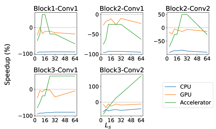
Figure 4: Speedup of PQ vs conventional convolution on different hardware when run on unique layers of ResNet20. A complete layer description is shown in Table 6.

Amortizing and reducing encoding costs. Computing the distances $\mathbf{d}^{(n)}$ between input columns and prototypes in the $n$-th subspace might come at a too high cost given that PQ only makes use of the index of the closest prototype to each column and not its actual value. A less computationally demanding distance could be used and we explore this in App. E.1. Alternatively, we could further leverage $\mathbf{d}^{(n)}$ and better amortise $\text{FLOPs}^{\text{enc}}$. To this end, we design a lightweight MLP corrector that, given these distances, it learns a transformation that helps further reducing $\text{MSE}^{\text{out}}$. Intuitively, the corrector has a higher potential for correction with longer and fewer prototypes. This is the pattern in Fig. 4 where we show the maximum observed reduction in $\text{MSE}^{\text{out}}$ across all layers in the study. Even though a well tuned corrector can still benefit PQ layers with short prototypes, its computational footprint for a given hidden dimension $h$, dominated by $N_{\text{s}}N_{\text{p}}\!\times\!h$, does not justify its use. In Sec. 6.2 we revisit the trade-offs of the corrector in the context of full-model training.

5 Hardware Modeling for PQ

In this section we assess the efficiency of running PQ on CPUs and GPUs, and we argue that custom hardware is needed to fully assess the efficiency potential of PQ compared to conventional convolutions. We design a custom PQ hardware accelerator (PQA) on an FPGA and we discuss its strengths, efficiency trends, and limitations. Throughout this section, we will compare PQA to a canonical systolic array-based deep learning accelerator (DLA) for native convolutions [3] implemented on the same FPGA device, with the same area utilization as PQA for a fair comparison.

5.1 PQ Speedup on Different Hardware Platforms

We quantify the impact on latency of applying PQ to unique layers of ResNet20 [45] on a CPU, GPU and custom hardware for each method. Our baseline custom hardware is DLA for native convolutions [3], and for PQ, we use our novel PQA accelerator, detailed later in this section. Fig 4 shows the speedup percentage for the unique layers of the network, obtained by running PQ and conventional convolution on different hardware and comparing the latencies. We sweep different values of $L_{\text{s}}$ while $N_{\text{p}}$ is kept at 16. It is clear that there is a consistent slowdown when running PQ on a CPU or a GPU as there is no speedup for different values of $L_{s}$ and the same observation appears when trying different values of $N_{\text{p}}$. Measuring the effect of PQ on commodity hardware like CPUs or GPUs is therefore a poor way of assessing its acceleration potential. However, using a custom hardware that is specifically designed for PQ achieves improvements in latency for certain configurations over DLA [3, 1]. While this is not the case in all layers, the speedup reaches up to $200\%$ in the last layer of the network at a large value of $L_{s}$.

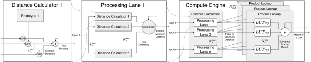
Figure 5: Block diagram of PQA, the proposed custom hardware implementation for PQ.

5.2 PQ Accelerator (PQA) Custom Hardware Design

Rather than relying on multiply-accumulate operations to calculate the result of a matrix-matrix multiplication, PQ performs memory lookups of precomputed results. This requires designing hardware that can perform these lookups efficiently. Luckily, PQ has many hardware-friendly properties that can make a custom hardware design efficient. (1) Because subspaces are completely independent, we can leverage that to partition the large product table (LUT${}_{\text{PQ}}$) memory across multiple small on-chip memories that allow parallel memory accesses. (2) The compute-heavy distance computation, to find the closest prototype, needs to be done only once regardless of the number of output channels. (3) With the exception of distance calculation, all other operations do not require heavy computations as they are either memory lookups or accumulations.

Fig. 5 shows the architecture of PQA: our novel compute engine that can be used to perform PQ inference. The engine consists of 3 main modules: A distance calculation module is responsible for determining the indices of the prototypes that are closest to the corresponding inputs. Next, the product lookup module consists of a partitioned memory array that is responsible for looking up the product of the closest prototype and the current weight for each subspace. Finally, the accumulator is responsible for adding results from different subspaces and producing the final outputs. Note that our results in this section use a DDR4 external memory chip with 36 GB/s transfer speeds, even though FPGAs (similar to GPUs/TPUs) are now available with high-bandwidth memory (HBM) that can reach up to 460 GB/s. We provide more analysis of HBM in Appendix K and in Section 6.

PQA is organized into processing lanes, replicated $N_{\text{s}}^{vec}$ times to process subspaces in parallel. It is also able to produce $N_{out}^{vec}$ outputs at a time by further breaking down the large LUT${}_{\text{PQ}}$ into smaller memories as shown in Fig. 5. As for inputs, the distance calculation module compares the input with $N_{\text{p}}^{vec}$ prototypes at a time where it compares $L_{\text{s}}^{vec}$ elements of the prototype each cycle.

The Compute Engine receives $L_{s}^{vec}$ portions of the input every cycle to be compared to all available prototypes, and to find the closest one. The index of the closest prototype is then sent to the product lookup portion that iterates over all weights, looks up the precomputed partial dot products, and accumulates these to compute each output. The product table memory is partitioned into $N_{s}^{vec}$ different banks to allow parallel lookups for each subspace. Furthermore, each subspace’s LUT is partitioned into $N_{out}^{vec}$ different memories—each handles a different set of output channels—to further parallelize product lookup and to produce multiple outputs simultaneously. PQA is therefore able to perform $N_{out}^{vec}\times N_{s}^{vec}$ LUT${}_{\text{PQ}}$ lookups in parallel. This custom on-chip memory hierarchy is key to PQA’s acceleration, and is not achievable with commodity hardware. Finally, results are accumulated across subspaces using a set of parallel accumulators repeated $N_{out}^{vec}$ times. See App. G, F, and J for more hardware details.

5.3 Layerwise Performance Analysis on PQA

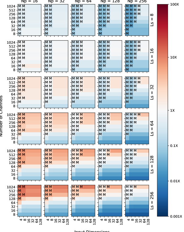
Figure 6: Speedup of different configurations of $N_{\text{p}}$, $L_{\text{s}}$, input dimensions and channels when considering a 3$\times$3 kernel on PQA and DLA. M = Memory Bound.

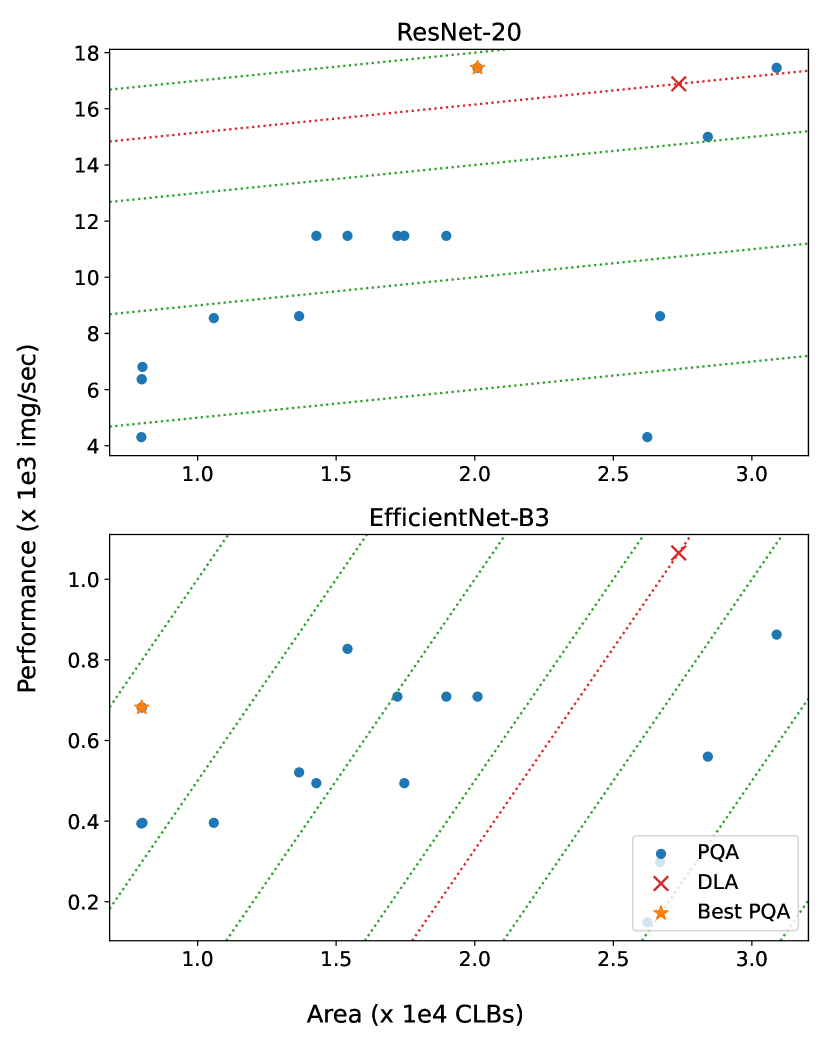
Figure 7: Performance vs area for different configurations of PQA for ResNet20 and EfficientNet-B3. Best DLA configurations are plotted for reference. Dotted lines represent constant performance per area.

Fig. 7 shows the speedup of running a convolution layer using PQ on a custom PQA compared to running its non-PQ equivalent on a custom DLA. The PQA has all vectorization parameters set to $16$ and its area is similar to the area of the custom DLA (only 4% larger). The convolution is done with a kernel of size 3$\times$3 and the number of input channels is assumed to be the same as the number of output channels.

As expected, smaller $N_{\text{p}}$ leads to faster PQ execution as the cycles needed to compare prototypes are fewer. Larger $N_{\text{p}}$ increases the LUT${}_{\text{PQ}}$ size and the time needed to load it from external memory, causing more points to become memory-bound. When increasing $L_{\text{s}}$, the number of subspaces ($N_{\text{s}}$) decreases and speeds up overall execution—we observe speedups starting from $L_{\text{s}}\!=\!32$. Finally, we can see that larger layers benefit more from PQ with speedups up to 100$\times$ at small $N_{\text{p}}$. In general, more aggressive PQ quantization leads to less computation and memory and therefore a better speedup. It is clear that running PQ on custom hardware is not a silver bullet, especially when compared to an optimized DLA. However, we have shown that unlike CPUs and GPUs, we are able to find parameters for which PQ can indeed outperform conventional convolutions.

6 Experimental Evaluation

Sections 4 and 5 presented a detailed analysis of the impact of PQ in a per-layer basis. This section studies those aspects at the model level: we report accuracy, memory footprint, theoretical compute footprint and cycles count for each model architecture. All details about our experimental setup, including training setup, dataset, architectures and hardware setup are in Appendix C.

6.1 End-to-End Model Performance on PQA

We measure the efficiency of running the two convolutional networks: ResNet20 and EfficientNet-B3 [52] on PQA vs. DLA. For ResNet20, we choose the PQ parameters $N_{\text{p}}=16$ and $L_{\text{s}}=9$ because they achieve the best accuracy as shown in Table 2. While for EfficientNet-B3, we only evaluate the hardware efficiency with the reasonable values of $N_{\text{p}}=16$ and $L_{\text{s}}=32$. As shown in Fig 7, it is important to choose the correct combination of the hardware parameters($N_{out}^{vec}$, $N_{\text{s}}^{vec}$, $N_{\text{p}}^{vec}$, $L_{\text{s}}^{vec}$) to achieve a better performance with less area. For Resnet20, the value that achieves best latency while staying less than DLA in area in this case happens to be at $N_{out}^{vec}=32$, $N_{\text{s}}=16$, $N_{\text{p}}^{vec}=16$, $L_{\text{s}}^{vec}=9$. There are some other configurations that achieve a higher performance but use much more area (not shown on the graph). For EfficientNet-B3, while DLA achieves the highest absolute performance, many of the configurations of PQA hardware parameters achieve better performance per area. The best PQA is roughly $2.2\times$ better than DLA in terms of performance per area.

6.2 Evaluating PQ Robustness for Model Quantization

The line plot in Fig. 8 shows the performance of MicroNet-PQ under varying configurations with just a 0.3% gap compared to the non-PQ baseline when {$N_{\text{p}}\!=\!16$, $L_{\text{s}}\!=\!4$}. The accompanying heat maps highlight different trade-offs between MicroNet-PQ and their non-PQ counterpart. When the accuracy requirement is lower, longer prototypes (higher $L_{\text{s}}$) can be selected to achieve a better FLOPs speedup ratio. With corrector, part of the degradation introduced by longer prototypes can be reduced in some cases by up to 7.3pp at a small memory footprint increase.

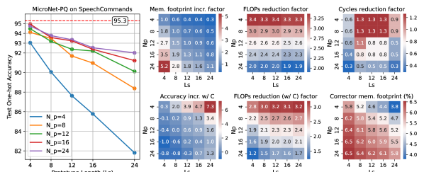
Figure 8: MicroNet-PQ reaches 95.0% accuracy with {$N_{\text{p}}\!=\!16$,$L_{\text{s}}\!=\!4$} leading to a $2.4\times$ reduction in the number of inference FLOPs. However, fewer FLOPs does not always translate in faster inference (cycles). When increasing memory footprint is not possible ({$N_{\text{p}}\!=\!8$, $L_{\text{s}}\!=\!8$}), Micronet-PQ still reaches over 93.5% while resulting in nearly $3\times$ lower computational footprint. With the corrector (displayed as ‘w/C‘), models with longer prototypes can reach that threshold accuracy too, at a small increase in memory footprint and FLOPs.

Table 2: Results of our PQ on ResNet20 and DW${}_{\text{EMNIST}}$ networks. Hardware latency is shown for DLA (baseline) and PQA for two differerent external memory chips: DDR4 and HBM with 36 GB/s and 460 GB/s bandwidth respectively. For ResNet20, DLA area is 36% larger than our PQA for the used configuration as shown in Fig. 7. For $DW_{EMNIST}$, our PQA area for the used configuration is 15% larger than DLA.

Model	Setting	$L_{\text{s}}$	$N_{\text{p}}$	Param.	Acc. (%)	Latency (Cycles)
						DDR4	HBM
ResNet20	Baseline	-	-	269k	92.6	17.7k	17.7k
	PECAN-D	3	64	5.7M	87.9	200k	124k
		9	64	1.93M	85.0	68k	41.5k
	Ours (PQ)	3	8	714k	83.9	38.4k	35.3k
		3	16	1.4M	82.4	49.9k	35.3k
		9	8	239k	84.1	13k	11.8k
		9	16	476k	84.4	17k	11.8k
DW${}_{\text{EMNIST}}$	Baseline	-	-	1.1M	90.4	1960	1557
	Ours (PQ)	4	8	2.1M	87.1	3528	2612
		4	12	3.1M	87.6	4312	2612
		4	16	4.0M	86.0	5227	2612
		8	8	1.1M	85.8	1976	1502
		8	16	2.1M	86.5	2792	1502
		16	16	1.1M	85.2	3184	3004

Results for full-model EMNIST training and for CIFAR-10 using ResNet20 are shown in Tab. 2. For the latter and {$N_{\text{p}}\!=\!16$, $L_{\text{s}}\!=\!9$}, we achieve 4$\times$ fewer cycles than PECAN-D at the cost of just 0.6% accuracy drop. For shorter prototypes ($L_{\text{s}}\!=\!3$) our models did not perform as good, even when increasing $N_{\text{p}}$ (an effect that also manifests in some EMNIST configurations). We provide some hypothesis on why this happens and mitigation we experimented with in Appendix C.3.

6.3 Evaluating PQ Acceleration Potential

Fig. 8 highlights the theme of our analysis in Section 5: FLOPs and memory footprint are not a good proxy for hardware latency for PQ as shown in the top 3 heatmaps of the figure. Indeed, many hardware implementation details eventually leads to a speedup for PQ, most importantly, the partitioned on-chip PQ LUT, and the parallel processing lanes for distance calculation. All considered, we were able to, for the first time, demonstrate a hardware speedup (+3% (DDR4) to 50% (HBM) on ResNet20) for PQ workloads, even when comparing against an optimized systolic array-based DLA as shown in Table 2. As expected, the faster HBM memory alleviates the memory bottleneck with PQ workloads and achieves higher speeds. When normalizing for area, PQA achieves 40% (DDR4) to 104% (HBM) higher perf/area compared to DLA on ResNet20. We demonstrate that it is possible to realize actual gains for PQ on hardware.

7 Conclusion

In this work we have identified several practical limitations that prevent PQ from been treated like other, more mature, optimizations techniques for model acceleration. As evidenced throughout our study, PQ requires a careful tuning to avoid incurring large overheads, especially in terms of memory and compute footprint. Unlike CPUs and GPUs, our custom hardware PQA has demonstrated that PQ can indeed accelerate entire models but not as much as higher-level proxy metrics such as FLOPs might suggest. PQA is faster than a conventional DLA by 3% in terms of performance, and 40% in performance/area on ResNet20, with much higher speedups when using faster HBM memory. To our knowledge, this is the first time a hardware speedup for PQ was demonstrated on any hardware platform. Furthermore, by codesigning PQ parameters and hardware, our PQ ResNet20 is 4$\times$ faster than the most recent PQ work with just 0.6% lower accuracy. With further hardware optimizations and more advanced PQ training methodologies, we believe that there is a high potential for achieving much larger hardware speedups for the emerging field of PQ for DNNs. In the future, we plan to investigate more robust and faster methods for PQ training, and the combination of PQ with other complementary compression methods such as scalar quantization and channel pruning.

8 Funding Disclosure

Funding for the Cornell University authors on this project is provided by Intel Corporation. The authors would like to thank Deshanand Singh, Susanne Balle, Mahesh Iyer, Nilesh Jain, Aravind Dasu, Gregg Baeckler, and Ilya Ganusov for insightful discussions and feedback.

Supplementary Material

Appendix A Limitations and Future Work

In this work we made use of PQ to accelerate relatively small ML models for image classification and keyword spotting. Their size and complexity allowed us to consider a broad range of experiments, including an extensive per-layer analysis. An obvious extension of our work would be to apply PQ to much larger models that, as evidenced by our hardware analysis in Section 5 and Table 7, far larger speedups are attainable with longer prototypes and a higher number of input channels. Regularity in the shapes of inputs and weights across layers in the network is also desirable for hardware design. Several modern architectures meet these two criteria (i.e. large and regular), for example ViT [13] and MLPMixer [53].

Often, models running on specialised hardware are not in FP32 precision. However, models obtained from our training pipeline are still in FP32. We argue that because of the very aggressive quantization that PQ applies, implementing a fully quantized (e.g. down to 16-bit or 8-bit) PQ pipeline would only introduce a small degradation (if at all). The reason for this is twofold: (1) the ranking of distances between input and prototypes is what really matters and not the values of these; (2) the table of pre-computed dot-products LUT${}_{\text{PQ}}$ can still be generated with FP32 weights and only afterwards, quantize it to the desired bit-width before deployment. Nevertheless, we find this an interesting research direction to expand our study.

The use of PQ is complementatry to other forms of accelerating inference. For example, using quantization (as briefly mentioned in the previous paragraph) could be used to reduce the computational footprint of the encoding stage as well as the overheads of storing and reading from LUT${}_{\text{PQ}}$. Structured pruning, in particular channel pruning [25, 6], can be applied first to a model and then obtain its PQ representation. With channel pruning, the number of output channels is reduced and so is the acceleration potential of PQ. This was shown analytically in Eq. 2 and empirically in Figure 7.

Appendix B Motivation++

Product quantization accelerates inference by replacing convolutions (and in general any type of layer doing matrix-matrix multiplication) by a series of look-ups to a table (a memory) of pre-computed dot-products. Acceleration is therefore achieved by reducing the computational footprint of compute intensive layers (i.e. convolutions in our work). This of course can be achieved by other methods such as standard element-wise quantization (i.e. going from 32-bit to INT8) or via pruning (i.e. discarding model parameters). In our work, we do not follow those standard methodologies and instead make a more radical change to the underlying computational graph representing the model: replace core operators (e.g convolutions) entirely with a series of lookups.

As shown in previous works [7, 45], PQ has a big potential but it remains unclear how to use it to accelerate all layers in the network without incurring into either severe model degradation or heavy memory footprint. Previous work (PECAN) focused on showing the potential of PQ but disregarded its trade-offs and did not evaluate whether it can actually result in acceleration and results in model artifacts many times larger than the original (non-PQ) model (as shown in Table  1). As we demonstrate in our work, accounting for FLOPs only is not a guarantee for speedups. This is because PQ replaces compute with memory accesses, and these are not captured when reporting FLOPs. Our work is the first to provide such analysis, which is fundamental for future work proposing alternative PQ implementations (for example new encoding functions, more lightweight distance metrics, new formulations of the corrector, etc).

In the limit, models with PQ will require orders of magnitude less compute to process an input because most of this compute will be pre-computed during training and stored in the look-up tables. What does this mean in practice? One example is that running models that are too demanding for the hardware can run them if sufficient memory to hold the look-up tables is available. To realise this, solid foundations on the trade offs of PQ need to be understood. That’s the motivation for our work. With our study we were able to present the first accelerator design capable of running PQ workloads and demonstrate actual speedups.

Appendix C Experimental Setup

Here we provide a detailed description of the models, dataset, hyperparameters and training schemes used in our per-layer study in Sec. 3.3 and full-model results in Sec. 6.

C.1 Model Architectures

The per-layer study in Sec. 4 made use of a CNN with 10 depth-wise separable layers. We designed this network, that we name $\text{DW}_{\text{EMNIST}}$, to be lightweight but deep enough so we could conduct the study considering a very large set of PQ-related parameters, {$N_{\text{p}}$, $L_{\text{s}}$, $\tau$}, and training related hyperparamters (batch sizes, learning rates, etc). A detailed description of the network is presented in Table 4. This network has a total of 1.05M paramters and requires 50.1M FLOPs when implemented as im2col. In Sec. 6 we analyse how a NAS-optimized MicroNet [4] for keyword spotting performs under different PQ settings. We refer to this network as MicroNet-PQ and a per-layer breakdown of parameters and shapes is provided in Table 5. This MicroNet baseline is an INT8 model designed to be run on microcontrollers. The last model considered in this work is a ResNet20 [24] for CIFAR-10. This is the same model evaluated in PECAN [45], and Table 6 provides a detailed view of this architecture.

C.2 Datasets

We make us of two image classification datasets: CIFAR-10 [37] and EMNIST [11]. The former is comprised of 50K $32\!\times\!32$ RGB images for training and 10K for testing, with both sets evenly split along ten image classes. The EMNIST dataset on the other hand is much larger totaling 112,800 and 18,800 images for training and testing respectively. We use the balanced partitioning of EMNIST which contains $28\!\times\!28$ greyscale images of digits and letters resulting in 47 classes with, as the name suggest, the same number of examples. The current best performing architecture on this dataset reaches 91.06% [31] in this partition. For both training sets we randomly leave 10% out for validation. For keyword spotting we rely on the SpeechCommands [59] data which is comprised of 105,829, 16KHz 1-second long audio clips of a spoken word (e.g. "yes", "up", "stop") and the task is to classify these correctly into 12 possible classes. Similar to previous works [64, 5, 4] we pre-process each audio clip and extract 10 MFCC [12] features using a 40ms window with a 20ms stride resulting in 10$\times$49 input matrices.

C.3 Training setup

We implement our training infrastructure with PyTorch [43]. We use two optimizers: one for the bank of prototypes in each layer $\mathbf{B}_{l}$; and another for the rest of the parameters in the model (e.g. the layer weights, and non-PQ layers.). Both instantiate an Adam optimizer [35] albeit with different learning rate. There are also two learning rate schedulers, each with its own decaying coefficient and scheduling. The hyperparameters for each model are presented in Table 3. We found learning rates and scheduling parameters to have large impact, not only in final model quality, but also in terms of training stability.

Table 3: Hyperparametrs used in our experiments. Due to the large space of PQ configurations and $\tau$ values considered, there is not a single golden config for each model. Here we report the ranges of hyperparemters that we found to deliver good quality models across PQ settings. Column Early Stop $\tau$ indicate the epoch from which temperature $\tau$ is kept fixed for the remaining of the training.

Model	Epochs	Batch	LR (params)	LR (proto)	Start $\tau$	End $\tau$	Early Stop $\tau$	Scheduler
DW${}_{\text{EMNIST}}$	90	96	[0.000,…,0.001]	[0.005,…,0.05]	1.0	0.0005	10	StepLR [30,50,70]
ResNet20	120	64	[0.005,…,0.05]	[0.025,…,0.075]	1.0	0.0005	10	StepLR [40,60,90]
MicroNet-PQ	30	96	[0.001,…,0.01]	[0.001,…, 0.025]	1.0	[0.0005, 0.001]	10	ExponentialLR [0.25,…,2.0]

A number of training techniques and tricks were considered and introduced to our training pipeline. We found gradient clipping to be crucial when training deeper models (i.e. ReseNet20 and DW${}_{\text{EMNIST}}$). Value-based gradient clipping [63] with small thresholds (e.g. 0.25, 0.5) alleviated exploding gradients in some cases. During the first epochs of training, the encoded input is obtained with $\tau$ values (see Eq. 1) that are gradually decreased. As it becomes smaller, the construction of the prototyped input gets close to one-hot, impacting the flow of gradients. We implemented two mechanisms to counteract this while still ensuring the performance of one-hot encoding is not affected: formulating the prototype selection in Eq. 1 via a Gumbel-Softmax [29]. This, however didn’t seem to have a clear impact on the quality of our training. What did have a small positive impact was to introduce an stochastic masking to the final encoded input $\mathbf{\hat{X}^{\text{enc}}}_{n,j}$ prior to multiplying it with the layer weights. This masking, applied at the sub-space level and individually to input column, allowed a fraction $\rho$ of vectors to remain unencoded (i.e. not changed by Eq. 1). We found that small $\rho\!=\!0.1$ lead to higher final one-hot PQ accuracy. Higher values would prevent layer weights and prototypes to adequately operate in one-hot scenarios, as it is the case during inference.

During inference, each column in each sub-space is one-hot encoded with its closest prototype instead of performing a linear combination of these. We use the index of this each prototype that minimises the distance metric $d(\cdot)$ (in our case we always train with Euclidean distance) to retrieve the precomputed dot-product in LUT${}_{\text{PQ}}$. This table is generated at the end of training.

In Section 6 we noted that in some cases, a higher number of prototypes did not lead to higher model accuracy. Our hypothesis is that at higher $N_{\text{p}}$ values, prototypes fail to capture distinctive enough aspect of the vectors in their respective sub-spaces. To counteract this we add a new term to our Cross Entropy training loss that encourages prototypes within a subspace to be orthogonal to each other [8]. We only found this regularization term to be useful to lessen the impact of sub-optimal training hyperparamters.

Table 4: The $\text{DW}_{\text{EMNIST}}$ architecture used in the per-layer study in Sec. 4 designed for EMNIST image classification. Pointwise convolutions dominate the compute footprint of this model. Because of this, only point-wise convolutions are considered to be replaced with PQ – for which we show the shapes of unrolled inputs and weights. This model has a total of 1.05M parameters and requires 50.1M FLOPs per $1\!\times\!28\!\times\!28$ input.

Layer	Input Shape	Unrolled Inputs	Unrolled Weights	Parameters	FLOPs	FLOPs (%)
Conv	[1, 1, 28, 28]	–	–	640	1,003,520	2.00
DepthW-1	[1, 64, 28, 28]	–	–	576	225,792	0.45
PointW-1	[1, 64, 14, 14]	[1, 64, 196]	[96, 64]	6,144	2,408,448	4.81
DepthW-2	[1, 96, 14, 14]	–	–	864	338,688	0.68
PointW-2	[1, 96, 14, 14]	[1, 96, 196]	[120, 96]	11,520	4,515,840	9.01
DepthW-3	[1, 120, 14, 14]	–	–	1,080	423,360	0.85
PointW-3	[1, 120, 14, 14]	[1, 120, 196]	[150, 120]	18,000	7,056,000	14.08
DepthW-4	[1, 150, 14, 14]	–	–	1,350	132,300	0.26
PointW-4	[1, 150, 7, 7]	[1, 150, 49]	[187, 150]	28,050	2,748,900	5.49
DepthW-5	[1, 187, 7, 7]	–	–	1,683	164,934	0.33
PointW-5	[1, 187, 7, 7]	[1, 187, 49]	[234, 187]	43,758	4,288,284	8.56
DepthW-6	[1, 234, 7, 7]	–	–	2,106	206,388	0.41
PointW-6	[1, 234, 7, 7]	[1, 234, 49]	[292, 234]	68,328	6,696,144	13.37
DepthW-7	[1, 292, 7, 7]	–	–	2,628	84,096	0.17
PointW-7	[1, 292, 4, 4]	[1, 292, 16]	[366, 292]	106,872	3,419,904	6.83
DepthW-8	[1, 366, 4, 4]	–	–	3,294	105,408	0.21
PointW-8	[1, 366, 4, 4]	[1, 366, 16]	[457, 366]	167,262	5,352,384	10.68
DepthW-9	[1, 457, 4, 4]	–	–	4,113	131,616	0.26
PointW-9	[1, 457, 4, 4]	[1, 457, 16]	[572, 457]	261,404	8,364,928	16.70
DepthW-10	[1, 572, 4, 4]	–	–	5,148	41,184	0.08
PointW-10	[1, 572, 2, 2]	[1, 572, 4]	[512, 572]	292,864	2,342,912	4.68
Linear	[1, 512]	–	–	24,111	48,222	0.10

Table 5: The MicroNet-PQ architecture designed for the SpeechCommands dataset. Pointwise convolutions dominate the compute footprint of this model, accounting for almost 75% of the FLOPs. Because of this, only point-wise convolutions are considered to be replaced with PQ – for which we show the shapes of unrolled inputs and weights. This model has a total of 60.6K parameters and requires 17.01M FLOPs per $1\!\times\!10\!\times\!49$ input. This model corresponds with MicroNet-KWS-S [4]. We modified the number of channels of the second depth-wise block from 112 to 120 so it’s divisible with common $\text{L}_{\text{s}}$ choices used throughout this work.

Layer	Input Shape	Unrolled Inputs	Unrolled Weights	Parameters	FLOPs	FLOPs (%)
Conv	[1, 1, 10, 49]	–	–	3,444	3,375,120	19.75
DepthW-1	[1, 84, 10, 49]	–	–	756	189,000	1.11
PointW-1	[1, 84, 5, 25]	[1, 84, 125]	[120, 84]	10,080	2,520,000	14.75
DepthW-2	[1, 120, 5, 25]	–	–	1,080	270,000	1.58
PointW-2	[1, 120, 5, 25]	[1, 120, 125]	[84, 120]	10,080	2,520,000	14.75
DepthW-3	[1, 84, 5, 25]	–	–	756	189,000	1.11
PointW-3	[1, 84, 5, 25]	[1, 84, 125]	[84, 84]	7,056	1,764,000	10.32
DepthW-4	[1, 84, 5, 25]	–	–	756	189,000	1.11
PointW-4	[1, 84, 5, 25]	[1, 84, 125]	[84, 84]	7,056	1,764,000	10.32
DepthW-5	[1, 84, 5, 25]	–	–	756	189,000	1.11
PointW-5	[1, 84, 5, 25]	[1, 84, 125]	[196, 84]	16,464	4,116,000	24.08
Linear	[1, 196]	–	–	2,364	4,728	0.03

Table 6: The ResNet20 architecture for CIFAR-10. All layers in the network with the exception of the input convolution and output linear layer are replaced with their PQ counterparts in our evaluation. For these we show the shapes of unrolled inputs and weights. This model has a total of 268K parameters and requires 81.1M FLOPs per $3\!\times\!32\!\times\!32$ input.

Layer	Input Shape	Unrolled Inputs	Unrolled Weights	Parameters	FLOPs	FLOPs (%)
Conv	[1, 3, 32, 32]	–	–	432	884,736	1.09
Block1-Conv1	[1, 16, 32, 32]	[1, 144, 1024]	[16, 144]	2,304	4,718,592	5.82
Block1-Conv2	[1, 16, 32, 32]	[1, 144, 1024]	[16, 144]	2,304	4,718,592	5.82
Block1-Conv3	[1, 16, 32, 32]	[1, 144, 1024]	[16, 144]	2,304	4,718,592	5.82
Block1-Conv4	[1, 16, 32, 32]	[1, 144, 1024]	[16, 144]	2,304	4,718,592	5.82
Block1-Conv5	[1, 16, 32, 32]	[1, 144, 1024]	[16, 144]	2,304	4,718,592	5.82
Block1-Conv6	[1, 16, 32, 32]	[1, 144, 1024]	[16, 144]	2,304	4,718,592	5.82
Block2-Conv1	[1, 16, 32, 32]	[1, 144, 256]	[32, 144]	4,608	2,359,296	2.91
Block2-Conv2	[1, 32, 16, 16]	[1, 288, 256]	[32, 288]	9,216	4,718,592	5.82
Block2-Conv3	[1, 32, 16, 16]	[1, 288, 256]	[32, 288]	9,216	4,718,592	5.82
Block2-Conv4	[1, 32, 16, 16]	[1, 288, 256]	[32, 288]	9,216	4,718,592	5.82
Block2-Conv5	[1, 32, 16, 16]	[1, 288, 256]	[32, 288]	9,216	4,718,592	5.82
Block2-Conv6	[1, 32, 16, 16]	[1, 288, 256]	[32, 288]	9,216	4,718,592	5.82
Block3-Conv1	[1, 32, 16, 16]	[1, 288, 64]	[64, 288]	18,432	2,359,296	2.91
Block3-Conv2	[1, 64, 8, 8]	[1, 576, 64]	[64, 576]	36,864	4,718,592	5.82
Block3-Conv3	[1, 64, 8, 8]	[1, 576, 64]	[64, 576]	36,864	4,718,592	5.82
Block3-Conv4	[1, 64, 8, 8]	[1, 576, 64]	[64, 576]	36,864	4,718,592	5.82
Block3-Conv5	[1, 64, 8, 8]	[1, 576, 64]	[64, 576]	36,864	4,718,592	5.82
Block3-Conv6	[1, 64, 8, 8]	[1, 576, 64]	[64, 576]	36,864	4,718,592	5.82
Linear	[1, 64]	–	–	650	1,300	0.00

C.4 HW-Setup

The hardware is designed in C++. Vitis HLS is used to compile it into HDL. Vivado is then used to do full synthesis. The FPGA part used for synthesis is xcvu9p-flga2104-2-i for most of the data points with the exception of configurations of high values($L_{s}^{vec}=32$, $N_{p}^{vec}=32$ and $N_{s}^{vec}=32$) in Fig. 13 where part xcvu47p_CIV-fsvh2892-3-e is used because it has enough DSPs to cover needed operations under these configurations.

Appendix D Memory and Compute footprint of PQ

In Sec 3.3 we derived an expression for the speedup in terms of FLOPs achievable by PQ over im2col. In Fig 9 we show how that expression maps to different speedups when varying $N_{\text{p}}$, $L_{\text{s}}$, and $C_{\text{out}}$. Having fewer prototypes (i.e. a smaller $N_{\text{p}}$) has a larger impact than designing PQ with longer prototypes (i.e. larger $L_{\text{s}}$), although this is also desirable. Another important observation is that PQ might not always be faster than im2col. This is true for convolutional layers with few output channels ($C_{\text{out}}\!<\!64$) and a moderate number of prototypes per sub-space.

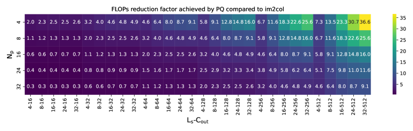
Figure 9: Reduction factor in the number of FLOPs when a layer with $C_{\text{out}}$ is implemented as a PQ layer with {$N_{\text{p}}$, $L_{\text{s}}$} parameterization. The speedup grows faster with $N_{\text{p}}$ than with $L_{\text{s}}$. For layers with very few output channels, there is no reduction in the number of FLOPs. Note this analysis assumes that looking-up the pre-computed dot product is cost free as discussed in Section 5.

Appendix E Extended per-layer Analysis

In Fig. 10 we show an extended version of the results first shown in Fig. 2 (bottom). Two main trends become evident in this visualisation. First, at deeper layers, where the spatial dimensions of the input tend to be smaller (i.e. leading to fewer columns in the unrolled input) the impact on Output MSE of having more prototypes, higher $N_{\text{p}}$, is less pronounced. For example, in layer 2 and short prototypes $L_{\text{s}}\!=\!4$ having $N_{\text{p}}\!=\!64$ compared to $N_{\text{p}}\!=\!8$ offers an Output MSE $2.4\times$ smaller. In layer 8, this difference is reduced to $1.7\times$. The second trend has to do with the costs of performing the input-to-prototype indexing, or in other words, computing the distance of each input column with the bank of prototypes in a given subspace (see Sec. 3.2). Due to the larger spatial dimensions in early layers in the network, the encoding costs $\text{FLOPS}^{\text{enc}}$ (refer to Sec. 3.3 for details) are much larger for a constant {$N_{\text{p}}$, $L_{\text{s}}$} configuration than in deeper layers. For example for {$N_{\text{p}}\!=\!64$, $L_{\text{s}}\!=\!8$}, $\text{FLOPS}^{\text{enc}}$ is $3.2\times$ larger in layer 2 and layer 8.

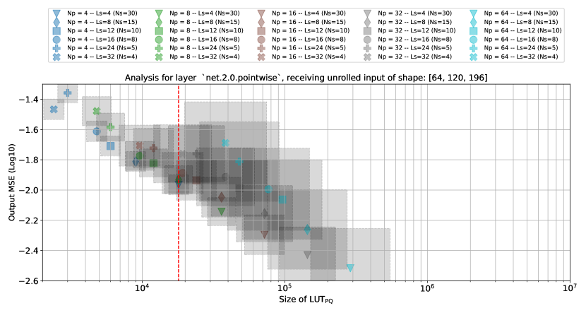
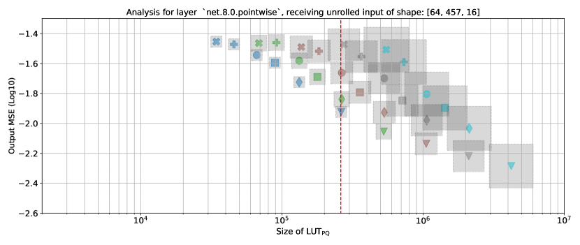
Figure 10: Analysis of the quality of the output generated by a PQ layer compared to the output of a non-PQ layer of a pre-trained model. The unit in the x-axis is number of parameters and we map to it the size of the resulting look up table, $\text{LUT}_{\text{PQ}}$, as well as the number of parameters that the same non-PQ layer has (this is shown as a vertical dashed red line). In addition to different memory footprints, each {$N_{\text{p}}$, $L_{\text{s}}$} pair also translates into different compute overheads when performing the input encoding. This is represented by the grey-shaded squares whose areas are proportional to $\text{FLOPS}^{\text{enc}}$. This is an extension to the results shown in Fig. 2.

E.1 Manhattan distance metric

The compute footprint analysis for PQ presented in Section 3.3, where we compare against im2col, accepts other distance metrics other than Euclidean distance. Here we show the impact of choosing Manhattan (L1) distance instead, which does not require multiplications.

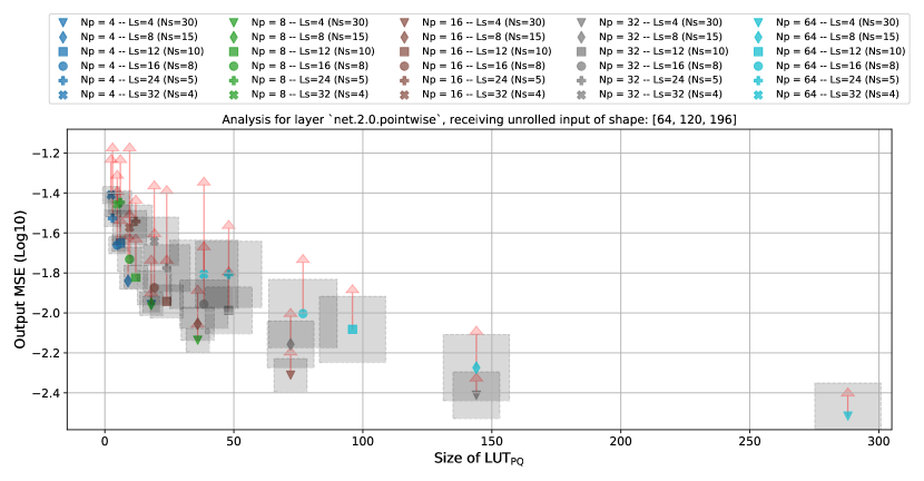
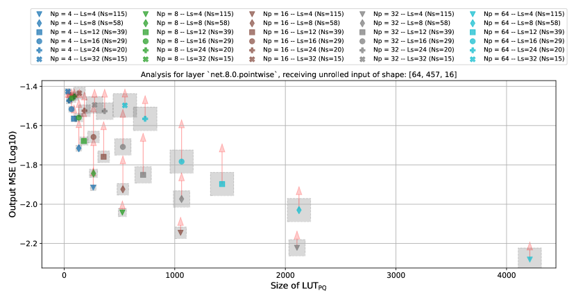
Figure 11: When replacing Euclidean distance with the more lightweight Manhattan distance, the error introduced to the output (represented as a red arrow) is not negligible with longer prototypes. The size of LUT${}_{\text{PQ}}$ is not affected by the choice of distance metric.

Appendix F Hardware extra plots

In Sec 5.1, we showed the speedup on different hardware platforms when changing the value of $L_{s}$. Fig 12 shows the same but when keeping value of $L_{s}$ at $16$ and changing the value of $N_{p}$. The same trends appear where CPU and GPU always show a slowdown while PQA shows sometimes speedup and sometimes slowdown.

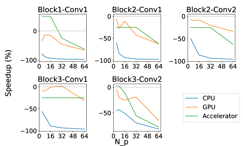
Figure 12: Speedup of PQ vs conventional conv on different hardware when run on unique layers of PECAN Network. The value of $L_{s}$ here is kept at 16 and the speedup with different values of $N_{p}$ are shown.

Appendix G Hardware description

A more detailed description of the hardware used is presented here.

The distance calculation module consists of many processing lanes, one per $N_{s}^{vec}$. The lane contains $N_{p}^{vec}$ difference calculators. Each difference calculator corresponds to a certain prototype. The lane receives an input which is $L_{s}^{vec}$ elements wide, passes it to all difference calculators, each producing the difference between this input and its corresponding prototype. These differences go to a comparator which is responsible for outputting the index of the prototype with the minimum distance from the input. The comparator needs to remember the minimum distance it has seen so far to compare it with upcoming distances from the next set of prototypes since the hardware is vectorized over $N_{out}^{vec}$.

Each difference calculator contains the elements of one prototype and is responsible for calculating the distance between the input and this specific prototype. It does that by passing each of the input elements along with its corresponding element in the prototype into the difference module then the output of all difference modules is added to an accumulator to produce the total distance. The accumulator is needed due to the vectorization of $L_{s}^{vec}$ which means that the difference calculated at each cycle might be partial for this prototype till the whole length of the prototype is processed, after which the outputted distance is the total.

One of the important considerations when designing a custom hardware is the area it requires. In this study, we express that in terms of the number of Configurable Logic Blocks(CLBs). We use the assumption that one DSP is equivalent to 3 CLBs and one BRAM is equivalent to 4 CLBs to convert all hardware resources to CLBs [46]. A simplified version of the described hardware is implemented where $N_{out}^{vec}$ is the only parameter that is less than the maximum supported number of outputs but other parameters are assumed to be equal to the maximum number of supported values. This eliminates the need for keeping history in the components and makes the design easier yet we believe that its area is representative of the area of the full design. The simplified version is synthesized and its area trends are shown in Fig 13. Each of the different hardware parameters is changed on a range of values from 4 to 32 while other parameters are kept at 16. It can be seen that $N_{s}^{vec}$, $L_{s}^{vec}$ and $N_{p}^{vec}$ have a high cost in terms of area while $N_{out}^{vec}$ doesn’t have as much cost when increasing. For the frequency, we assume PQA and DLA run at the same frequency.

Table 7 shows our hardware accelerator when synthesized using different parameters. It shows the results of post-synthesis results components usage along with the final equivalent CLBs.

Table 7: A table showing different hardware parameters and their post-synthesis results along with the calculated equivalent CLBs.

$N_{out}^{vec}$	$N_{\text{s}}^{vec}$	$L_{\text{s}}^{vec}$	$N_{\text{p}}^{vec}$	CLBs	BRAM	DSP	Equivalent CLBs
4	16	16	16	13426	128	4096	26226
8	16	16	16	13886	128	4096	26686
16	4	16	16	4643	64	1024	7971
16	8	16	16	7007	128	2048	13663
16	16	4	16	6489	256	1024	10585
16	16	8	16	10290	256	2048	17458
16	16	16	4	4427	128	1024	8011
16	16	16	8	7629	128	2048	14285
16	16	16	16	15098	256	4096	28410
16	16	16	32	23768	256	8192	49368
16	16	32	16	23919	256	8192	49519
16	32	16	16	28861	512	8192	55485
32	4	16	16	4658	64	1024	7986
32	4	16	16	4658	64	1024	7986
32	8	16	16	8753	128	2048	15409
32	16	8	16	11806	256	2048	18974
32	16	9	16	11405	256	2557	20100
32	16	16	8	10040	256	2048	17208
32	16	16	16	17581	256	4096	30893
64	4	16	16	9971	128	1024	13555
64	8	16	16	16453	256	2048	23621
64	16	8	8	27148	256	1024	31244

Appendix H Hardware Parameters Trends

Fig 13 shows how the area and the latency change as one of the hardware parameters is changed. It can be seen that $N_{out}^{vec}$ has a small effect on area but has a good effect on performance for the given network.

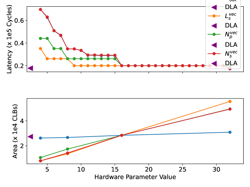
Figure 13: Performance(top) and Area(bottom) trends of the hardware parameters. The performance is measured in number of cycles needed to process an input through ResNet20 network and the area is measured in number of equivalent CLBs. All other parameters have their value set to 16 while the parameter in question is swept across the range.

Appendix I Layerwise Performance Analysis using Different Kernel Sizes

In this section, we show heatmaps similar to the one shown in 7 but evaluated on different Kernel sizes other than 3 ranging from 1 to 6. Cells labeled with $N$ are cells where cycles taken for compute are equal to cycles taken for memory. Heatmaps are shown in Figs 14,15,16,17,18

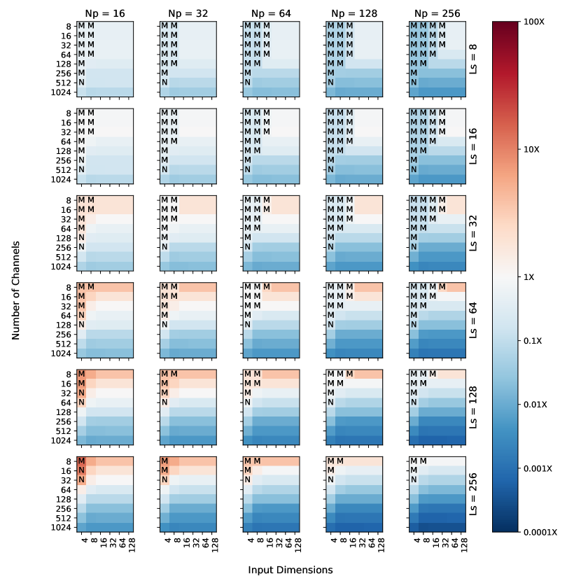
Figure 14: K = 1, using DDR memory

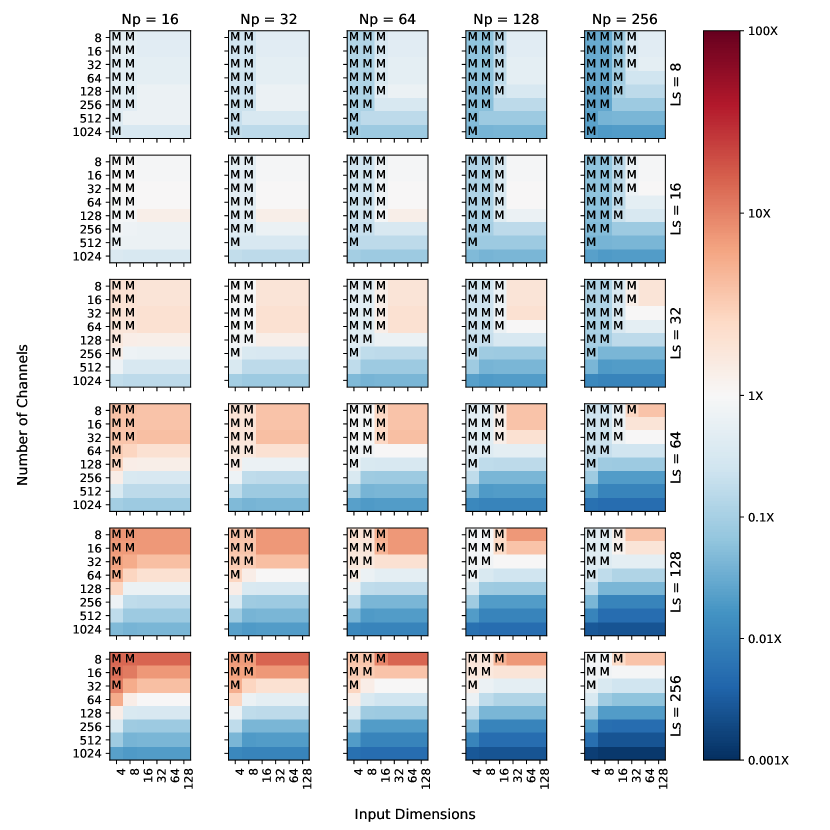
Figure 15: K = 2, using DDR memory

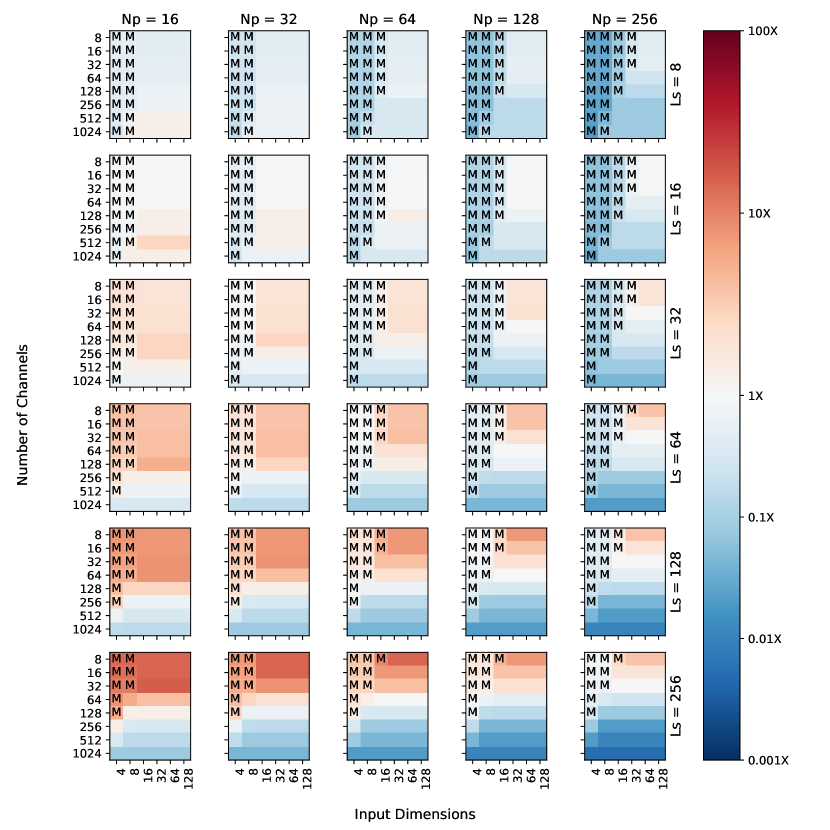
Figure 16: K = 4, using DDR memory

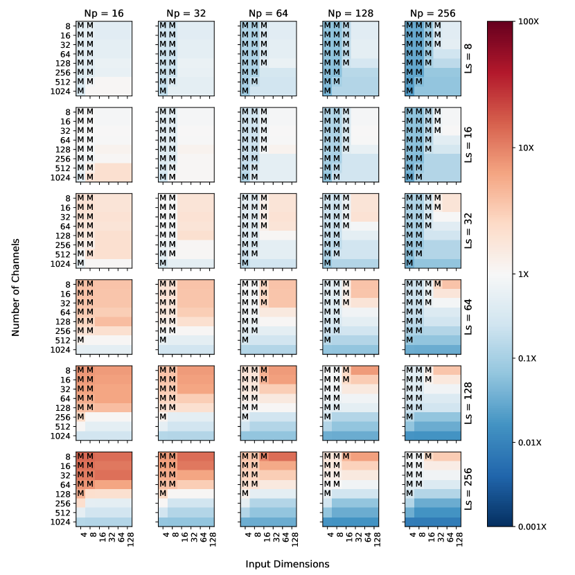
Figure 17: K = 5, using DDR memory

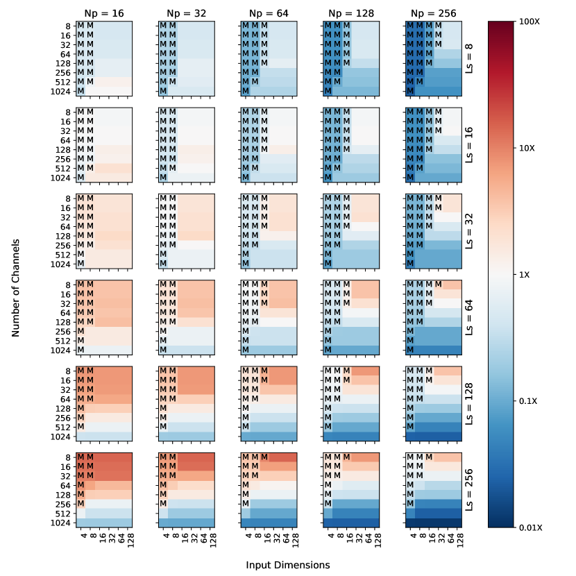
Figure 18: K = 6, using DDR memory

Appendix J Accuracy and hardware performance

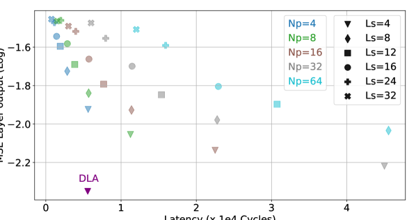
Figure 19: MSE in a sample layer output vs number of cycles needed to process the input.

To link our hardware efficiency study with PQ accuracy, Fig 19 plots the the mean square error (MSE) of the output vs. the number of PQA cycles for different PQ parameters for PointW-9 layer described in Table 4. It can be seen that increasing $N_{p}$ increases the accuracy marginally while it has a clearer effect on the cycle count especially for larger $L_{s}$. It is worth noting that in this case, the efficiency of the hardware is limited by the external memory bandwidth so increasing $N_{p}$ increases the size of the lookup table leading to more memory bandwidth requirements.

Appendix K HBM Analysis

In this section, we show plots that were previously done without a high bandwidth memory when done with both PQA and DLA use a high bandwidth memory. It can be seen in Fig. 20 that the memory bound points become less. Same is shown for other Kernel sizes in Figs 21,22,23,24,25

Figure 20: Speedup of different configurations of $N_{p}$, $L_{s}$, input dimensions and channels when doing convolution with a 3x3 kernel on the custom PQA and the custom DLA using HBM. M=Memory Bound.

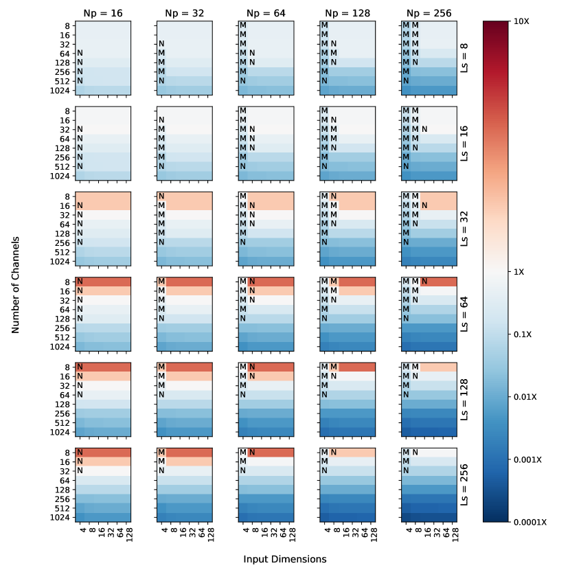
Figure 21: K = 1, using HBM

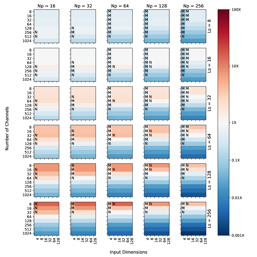
Figure 22: K = 2, using HBM

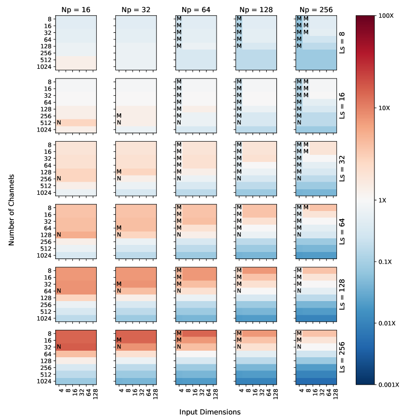
Figure 23: K = 4, using HBM

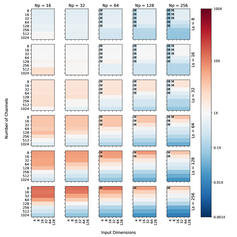
Figure 24: K = 5, using HBM

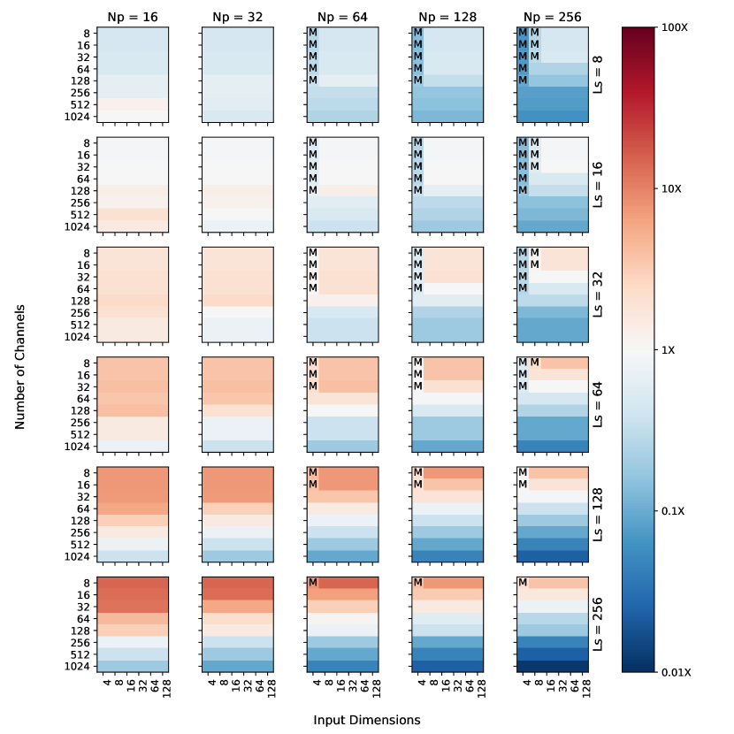
Figure 25: K = 6, using HBM

Fig. 26 shows the performance vs area for the 2 accelerators when run using HBM. It can be seen that the performance gap between the best PQA and the DLA increases heavily. This indicates that PQA makes better use of faster memory than DLA.

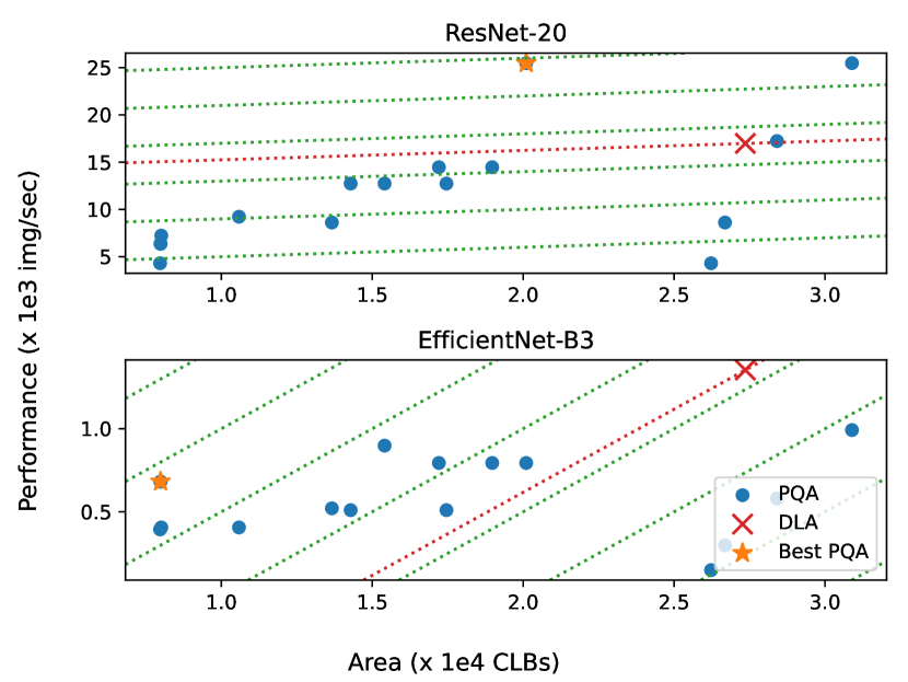
Figure 26: Performance vs area for different configurations of PQA for ResNet20 on the custom PQA and the custom DLA using HBM. Best DLA configuration is plotted for reference.

References

- [1] Mohamed S. Abdelfattah, David Han, Andrew Bitar, Roberto Dicecco, Shane O’Connell, Nitika Shanker, Joseph Chu, Ian Prins, Joshua Fender, Andrew C. Ling, and Gordon R. Chiu. DLA: Compiler and FPGA Overlay for Neural Network Inference Acceleration. 28th International Conference on Field Programmable Logic and Applications (FPL), pages 411–4117, 2018.
- [2] Dennis Abts, Jonathan Ross, Jonathan Sparling, Mark Wong-VanHaren, Max Baker, Tom Hawkins, Andrew Bell, John Thompson, Temesghen Kahsai, Garrin Kimmell, Jennifer Hwang, Rebekah Leslie-Hurd, Michael Bye, E. R. Creswick, Matthew Boyd, Mahitha Venigalla, Evan Laforge, Jon Purdy, Purushotham Kamath, Dinesh Maheshwari, Michael Beidler, Geert Rosseel, Omar Ahmad, Gleb Gagarin, Richard Czekalski, Ashay Rane, Sahil Parmar, Jeff Werner, Jim Sproch, Adrian Macias, and Brian Kurtz. Think fast: A tensor streaming processor (tsp) for accelerating deep learning workloads. In Proceedings of the ACM/IEEE 47th Annual International Symposium on Computer Architecture, ISCA ’20, page 145–158. IEEE Press, 2020.
- [3] Utku Aydonat, Shane O’Connell, Davor Capalija, Andrew C Ling, and Gordon R Chiu. An opencl™ deep learning accelerator on arria 10. In Proceedings of the 2017 ACM/SIGDA International Symposium on Field-Programmable Gate Arrays, pages 55–64, 2017.
- [4] Colby Banbury, Chuteng Zhou, Igor Fedorov, Ramon Matas, Urmish Thakker, Dibakar Gope, Vijay Janapa Reddi, Matthew Mattina, and Paul Whatmough. Micronets: Neural network architectures for deploying tinyml applications on commodity microcontrollers. In A. Smola, A. Dimakis, and I. Stoica, editors, Proceedings of Machine Learning and Systems, volume 3, pages 517–532, 2021.
- [5] Axel Berg, Mark O’Connor, and Miguel Tairum Cruz. Keyword Transformer: A Self-Attention Model for Keyword Spotting. In Proc. Interspeech 2021, pages 4249–4253, 2021.
- [6] Davis Blalock, Jose Javier Gonzalez Ortiz, Jonathan Frankle, and John Guttag. What is the state of neural network pruning? In I. Dhillon, D. Papailiopoulos, and V. Sze, editors, Proceedings of Machine Learning and Systems, volume 2, pages 129–146, 2020.
- [7] Davis Blalock and John Guttag. Multiplying matrices without multiplying. In Marina Meila and Tong Zhang, editors, Proceedings of the 38th International Conference on Machine Learning, volume 139 of Proceedings of Machine Learning Research, pages 992–1004. PMLR, 18–24 Jul 2021.
- [8] Andrew Brock, Theodore Lim, J. M. Ritchie, and Nick Weston. Neural photo editing with introspective adversarial networks, 2016.
- [9] Hanting Chen, Yunhe Wang, Chunjing Xu, Boxin Shi, Chao Xu, Qi Tian, and Chang Xu. Addernet: Do we really need multiplications in deep learning? In Proceedings of the IEEE/CVF Conference on Computer Vision and Pattern Recognition (CVPR), June 2020.
- [10] Yu-Hsin Chen, Tien-Ju Yang, Joel Emer, and Vivienne Sze. Eyeriss v2: A flexible accelerator for emerging deep neural networks on mobile devices. IEEE Journal on Emerging and Selected Topics in Circuits and Systems, 9(2):292–308, 2019.
- [11] Gregory Cohen, Saeed Afshar, Jonathan Tapson, and Andre Van Schaik. Emnist: Extending mnist to handwritten letters. 2017 International Joint Conference on Neural Networks (IJCNN), 2017.
- [12] S. Davis and P. Mermelstein. Comparison of parametric representations for monosyllabic word recognition in continuously spoken sentences. IEEE Transactions on Acoustics, Speech, and Signal Processing, 28(4):357–366, 1980.
- [13] Alexey Dosovitskiy, Lucas Beyer, Alexander Kolesnikov, Dirk Weissenborn, Xiaohua Zhai, Thomas Unterthiner, Mostafa Dehghani, Matthias Minderer, Georg Heigold, Sylvain Gelly, Jakob Uszkoreit, and Neil Houlsby. An image is worth 16x16 words: Transformers for image recognition at scale. In International Conference on Learning Representations, 2021.
- [14] Alaaeldin El-Nouby, Matthew J. Muckley, Karen Ullrich, Ivan Laptev, Jakob Verbeek, and Hervé Jégou. Image compression with product quantized masked image modeling, 2022.
- [15] H. Fan, T. Chau, S. I. Venieris, R. Lee, A. Kouris, W. Luk, N. D. Lane, and M. S. Abdelfattah. Adaptable butterfly accelerator for attention-based nns via hardware and algorithm co-design. In 2022 55th IEEE/ACM International Symposium on Microarchitecture (MICRO), pages 599–615, Los Alamitos, CA, USA, oct 2022. IEEE Computer Society.
- [16] H. Fan, T. Chau, S. I. Venieris, R. Lee, A. Kouris, W. Luk, N. D. Lane, and M. S. Abdelfattah. Adaptable butterfly accelerator for attention-based nns via hardware and algorithm co-design. In 2022 55th IEEE/ACM International Symposium on Microarchitecture (MICRO), pages 599–615, Los Alamitos, CA, USA, oct 2022. IEEE Computer Society.
- [17] Igor Fedorov, Ryan P Adams, Matthew Mattina, and Paul Whatmough. Sparse: Sparse architecture search for cnns on resource-constrained microcontrollers. In H. Wallach, H. Larochelle, A. Beygelzimer, F. d'Alché-Buc, E. Fox, and R. Garnett, editors, Advances in Neural Information Processing Systems, volume 32. Curran Associates, Inc., 2019.
- [18] Javier Fernandez-Marques, Paul Whatmough, Andrew Mundy, and Matthew Mattina. Searching for winograd-aware quantized networks. In I. Dhillon, D. Papailiopoulos, and V. Sze, editors, Proceedings of Machine Learning and Systems, volume 2, pages 14–29, 2020.
- [19] Tiezheng Ge, Kaiming He, Qifa Ke, and Jian Sun. Optimized product quantization. IEEE Transactions on Pattern Analysis and Machine Intelligence, 36(4):744–755, 2014.
- [20] Dibakar Gope, Jesse Beu, Urmish Thakker, and Matthew Mattina. Ternary mobilenets via per-layer hybrid filter banks. In Proceedings of the IEEE/CVF Conference on Computer Vision and Pattern Recognition (CVPR) Workshops, June 2020.
- [21] Junli Gu, Yibing Liu, Yuan Gao, and Maohua Zhu. Opencl caffe: Accelerating and enabling a cross platform machine learning framework. In Proceedings of the 4th International Workshop on OpenCL, IWOCL ’16, pages 8:1–8:5, New York, NY, USA, 2016. ACM.
- [22] Mathew Hall and Vaughn Betz. Hpipe: Heterogeneous layer-pipelined and sparse-aware cnn inference for fpgas. In Proceedings of the 2020 ACM/SIGDA International Symposium on Field-Programmable Gate Arrays, FPGA ’20, page 320, New York, NY, USA, 2020. Association for Computing Machinery.
- [23] Kaiming He, Xiangyu Zhang, Shaoqing Ren, and Jian Sun. Deep residual learning for image recognition. 2016 IEEE Conference on Computer Vision and Pattern Recognition (CVPR), Jun 2016.
- [24] Kaiming He, Xiangyu Zhang, Shaoqing Ren, and Jian Sun. Deep residual learning for image recognition. In Proceedings of the IEEE Conference on Computer Vision and Pattern Recognition (CVPR), June 2016.
- [25] Yihui He, Xiangyu Zhang, and Jian Sun. Channel pruning for accelerating very deep neural networks, 2017.
- [26] M. Horowitz. 1.1 computing’s energy problem (and what we can do about it). In 2014 IEEE International Solid-State Circuits Conference Digest of Technical Papers (ISSCC), pages 10–14, Feb 2014.
- [27] Benoit Jacob, Skirmantas Kligys, Bo Chen, Menglong Zhu, Matthew Tang, Andrew Howard, Hartwig Adam, and Dmitry Kalenichenko. Quantization and training of neural networks for efficient integer-arithmetic-only inference. 2018 IEEE/CVF Conference on Computer Vision and Pattern Recognition, Jun 2018.
- [28] Animesh Jain, Shoubhik Bhattacharya, Masahiro Masuda, Vin Sharma, and Yida Wang. Efficient execution of quantized deep learning models: A compiler approach, 2020.
- [29] Eric Jang, Shixiang Gu, and Ben Poole. Categorical reparameterization with gumbel-softmax, 2016.
- [30] Young Kyun Jang and Nam Ik Cho. Generalized product quantization network for semi-supervised image retrieval. In IEEE/CVF Conference on Computer Vision and Pattern Recognition (CVPR), June 2020.
- [31] Pranav Jeevan, Kavitha Viswanathan, Anandu A S, and Amit Sethi. Wavemix: A resource-efficient neural network for image analysis, 2022.
- [32] Yangqing Jia. Learning Semantic Image Representations at a Large Scale. PhD thesis, EECS Department, University of California, Berkeley, May 2014.
- [33] Norman P. Jouppi, Cliff Young, Nishant Patil, David Patterson, Gaurav Agrawal, Raminder Bajwa, Sarah Bates, Suresh Bhatia, Nan Boden, Al Borchers, Rick Boyle, Pierre-luc Cantin, Clifford Chao, Chris Clark, Jeremy Coriell, Mike Daley, Matt Dau, Jeffrey Dean, Ben Gelb, Tara Vazir Ghaemmaghami, Rajendra Gottipati, William Gulland, Robert Hagmann, C. Richard Ho, Doug Hogberg, John Hu, Robert Hundt, Dan Hurt, Julian Ibarz, Aaron Jaffey, Alek Jaworski, Alexander Kaplan, Harshit Khaitan, Daniel Killebrew, Andy Koch, Naveen Kumar, Steve Lacy, James Laudon, James Law, Diemthu Le, Chris Leary, Zhuyuan Liu, Kyle Lucke, Alan Lundin, Gordon MacKean, Adriana Maggiore, Maire Mahony, Kieran Miller, Rahul Nagarajan, Ravi Narayanaswami, Ray Ni, Kathy Nix, Thomas Norrie, Mark Omernick, Narayana Penukonda, Andy Phelps, Jonathan Ross, Matt Ross, Amir Salek, Emad Samadiani, Chris Severn, Gregory Sizikov, Matthew Snelham, Jed Souter, Dan Steinberg, Andy Swing, Mercedes Tan, Gregory Thorson, Bo Tian, Horia Toma, Erick Tuttle, Vijay Vasudevan, Richard Walter, Walter Wang, Eric Wilcox, and Doe Hyun Yoon. In-datacenter performance analysis of a tensor processing unit. SIGARCH Comput. Archit. News, 45(2):1–12, jun 2017.
- [34] Herve Jégou, Matthijs Douze, and Cordelia Schmid. Product quantization for nearest neighbor search. IEEE Transactions on Pattern Analysis and Machine Intelligence, 33(1):117–128, 2011.
- [35] Diederik P. Kingma and Jimmy Ba. Adam: A method for stochastic optimization, 2014.
- [36] Benjamin Klein and Lior Wolf. End-to-end supervised product quantization for image search and retrieval. In Proceedings of the IEEE/CVF Conference on Computer Vision and Pattern Recognition (CVPR), June 2019.
- [37] Alex Krizhevsky, Geoffrey Hinton, et al. Learning multiple layers of features from tiny images. 2009.
- [38] Andrew Lavin and Scott Gray. Fast algorithms for convolutional neural networks. 2016 IEEE Conference on Computer Vision and Pattern Recognition (CVPR), Jun 2016.
- [39] Edgar Liberis and Nicholas D. Lane. Neural networks on microcontrollers: saving memory at inference via operator reordering, 2019.
- [40] Calvin McCarter and Nicholas Dronen. Look-ups are not (yet) all you need for deep learning inference, 2022.
- [41] Sachin Mehta and Mohammad Rastegari. Mobilevit: Light-weight, general-purpose, and mobile-friendly vision transformer. In International Conference on Learning Representations, 2022.
- [42] Junting Pan, Adrian Bulat, Fuwen Tan, Xiatian Zhu, Lukasz Dudziak, Hongsheng Li, Georgios Tzimiropoulos, and Brais Martinez. Edgevits: Competing light-weight cnns on mobile devices with vision transformers. In European Conference on Computer Vision, 2022.
- [43] Adam Paszke, Sam Gross, Francisco Massa, Adam Lerer, James Bradbury, Gregory Chanan, Trevor Killeen, Zeming Lin, Natalia Gimelshein, Luca Antiga, Alban Desmaison, Andreas Kopf, Edward Yang, Zachary DeVito, Martin Raison, Alykhan Tejani, Sasank Chilamkurthy, Benoit Steiner, Lu Fang, Junjie Bai, and Soumith Chintala. PyTorch: An Imperative Style, High-Performance Deep Learning Library. In Advances in Neural Information Processing Systems (NeurIPS), pages 8026–8037, 2019.
- [44] Gabriele Prato, Ella Charlaix, and Mehdi Rezagholizadeh. Fully quantized transformer for machine translation, 2019.
- [45] Jie Ran, Rui Lin, Jason Chun Lok Li, Jiajun Zhou, and Ngai Wong. Pecan: A product-quantized content addressable memory network, 2022.
- [46] Rafat Rashid, J Gregory Steffan, and Vaughn Betz. Comparing performance, productivity and scalability of the tilt overlay processor to opencl hls. In 2014 International Conference on Field-Programmable Technology (FPT), pages 20–27. IEEE, 2014.
- [47] Mohammad Rastegari, Vicente Ordonez, Joseph Redmon, and Ali Farhadi. Xnor-net: Imagenet classification using binary convolutional neural networks. CoRR, abs/1603.05279, 2016.
- [48] Mark Sandler, Andrew Howard, Menglong Zhu, Andrey Zhmoginov, and Liang-Chieh Chen. Mobilenetv2: Inverted residuals and linear bottlenecks. 2018 IEEE/CVF Conference on Computer Vision and Pattern Recognition, Jun 2018.
- [49] Pierre Stock, Armand Joulin, Rémi Gribonval, Benjamin Graham, and Hervé Jégou. And the bit goes down: Revisiting the quantization of neural networks. In International Conference on Learning Representations (ICLR), 2020.
- [50] Zhiqing Sun, Hongkun Yu, Xiaodan Song, Renjie Liu, Yiming Yang, and Denny Zhou. Mobilebert: a compact task-agnostic bert for resource-limited devices. In ACL (2020), 2020.
- [51] Shyam Anil Tailor, Javier Fernandez-Marques, and Nicholas Donald Lane. Degree-quant: Quantization-aware training for graph neural networks. In International Conference on Learning Representations, 2021.
- [52] Mingxing Tan and Quoc V. Le. Efficientnet: Rethinking model scaling for convolutional neural networks, 2019.
- [53] Ilya Tolstikhin, Neil Houlsby, Alexander Kolesnikov, Lucas Beyer, Xiaohua Zhai, Thomas Unterthiner, Jessica Yung, Andreas Steiner, Daniel Keysers, Jakob Uszkoreit, Mario Lucic, and Alexey Dosovitskiy. Mlp-mixer: An all-mlp architecture for vision, 2021.
- [54] Michael Tschannen, Aran Khanna, and Animashree Anandkumar. StrassenNets: Deep learning with a multiplication budget. In Jennifer Dy and Andreas Krause, editors, Proceedings of the 35th International Conference on Machine Learning, volume 80 of Proceedings of Machine Learning Research, pages 4985–4994, Stockholmsmässan, Stockholm Sweden, 10–15 Jul 2018. PMLR.
- [55] Ashish Vaswani, Noam Shazeer, Niki Parmar, Jakob Uszkoreit, Llion Jones, Aidan N Gomez, Ł ukasz Kaiser, and Illia Polosukhin. Attention is all you need. In I. Guyon, U. Von Luxburg, S. Bengio, H. Wallach, R. Fergus, S. Vishwanathan, and R. Garnett, editors, Advances in Neural Information Processing Systems, volume 30. Curran Associates, Inc., 2017.
- [56] S. I. Venieris, I. Panopoulos, and I. S. Venieris. Oodin: An optimised on-device inference framework for heterogeneous mobile devices. In 2021 IEEE International Conference on Smart Computing (SMARTCOMP), pages 1–8, Los Alamitos, CA, USA, aug 2021. IEEE Computer Society.
- [57] Diwen Wan, Fumin Shen, Li Liu, Ling Shao, Jie Qin, and Heng Tao Shen. Tbn: Convolutional neural network with ternary inputs and binary weights. In ECCV, 2018.
- [58] Kuan Wang, Zhijian Liu, Yujun Lin, Ji Lin, and Song Han. Haq: Hardware-aware automated quantization with mixed precision. In The IEEE Conference on Computer Vision and Pattern Recognition (CVPR), June 2019.
- [59] Pete Warden. Speech commands: A dataset for limited-vocabulary speech recognition. arXiv preprint arXiv:1804.03209, 2018.
- [60] Paul N. Whatmough, Chuteng Zhou, Patrick Hansen, Shreyas Kolala Venkataramanaiah, J.-S. Seo, and Matthew Mattina. FixyNN: Efficient Hardware for Mobile Computer Vision via Transfer Learning, 2019.
- [61] Tan Yu, Junsong Yuan, Chen Fang, and Hailin Jin. Product quantization network for fast image retrieval. In Proceedings of the European Conference on Computer Vision (ECCV), September 2018.
- [62] Jialiang Zhang and Jing Li. Pq-cnn: Accelerating product quantized convolutional neural network on fpga. In 2018 IEEE 26th Annual International Symposium on Field-Programmable Custom Computing Machines (FCCM), pages 207–207, 2018.
- [63] Jingzhao Zhang, Tianxing He, Suvrit Sra, and Ali Jadbabaie. Why gradient clipping accelerates training: A theoretical justification for adaptivity. In International Conference on Learning Representations, 2020.
- [64] Yundong Zhang, Naveen Suda, Liangzhen Lai, and Vikas Chandra. Hello edge: Keyword spotting on microcontrollers, 2018.