Mass-redshift dependency of Supermassive Black Hole Binaries for the Gravitational Wave Background

Abstract

Studying how the black hole (BH) - (galaxy) bulge mass relation evolves with redshift provides valuable insights into the co-evolution of supermassive black holes and their host galaxies. However, obtaining accurate measurement of BH masses is challenging due to the bias towards the most massive and luminous galaxies. We use an analytical astrophysical model with galaxy stellar mass function, pair fraction, merger timescale and BH-bulge mass relation extended to include redshift evolution. The model can predict the intensity of the gravitational wave background produced by a population of supermassive black hole binary (SMBHB) as a function of the frequency. We focus on the BH-bulge mass relation and its variation with redshift using the EAGLE, Illustris, TNG100, TNG300, Horizon-AGN and SIMBA large-scale cosmological simulations. By understanding the processes and relationships concerning the formation and co-evolution of galaxies and their central BHs we can make theoretical and analytical expressions in order to refine current astrophysical models. This allows us to compare the predictions of this model with the constraints of Pulsar Timing Array observations. Here, we employ Bayesian analysis for the parameter inference. By fitting the BH-bulge mass parameters to the Illustris and SIMBA simulations we analyze the changes in the constraints on the other astrophysical parameters. Furthermore, we also examine the variation in SMBHB merger rate with mass and redshift between these large-scale simulations.

1 Introduction

The co-evolution of galaxies and their supermassive black holes (SMBHs), i.e. the relationship between SMBHs and the dark matter halo potential, their role in the stellar formation activity, their local interactions with the stars and gas, and their fate during the history of galaxy mergers, are key ingredients of recent large cosmological simulations and of our understanding of large-scale structure formation and evolution (see e.g. Habouzit et al., 2021, 2022a, and references therein).

Moreover, the SMBH pair formation process in the post-merger galaxy potential and their inspiral to coalescence, produces gravitational waves (GWs) in the low frequency domain, observable either as a stochastic gravitational wave background (GWB) or as individual continuous gravitational wave sources with Pulsar Timing Array (PTA) experiments (nHz$-\mu$Hz) (Foster & Backer, 1990; Rajagopal & Romani, 1995; Jaffe & Backer, 2003; Sesana et al., 2008), or with the future spatial laser interferometers like LISA ($10^{-4}$Hz$-10^{-2}$Hz) (Amaro-Seoane et al., 2017, 2023).

A PTA uses radio telescopes to time a network of millisecond pulsars (Sazhin, 1978; Detweiler, 1979). In principle, once the pulsar rotation irregularities, its possible orbital motion, the dispersion and scattering of its radio signal through the interstellar and heliospheric plasma and the systematics due to the Earth motion are properly modelled and subtracted from the time series of measured pulsations, one expects to be able to extract the GW imprint from the resulting timing residuals. The analysis requires observations of multiple millisecond pulsars at sub $\mu$s precision for several decades (up to about 25 years for ongoing programs) in order to extract a GWB from unmodelled noise. There are several PTA consortia, structured at continental levels and collaborating globally: European PTA (EPTA)(Kramer & Champion, 2013; Desvignes et al., 2016; Chen et al., 2021), Parkes PTA (PPTA) in Australia (Manchester et al., 2013; Hobbs, 2013; Kerr et al., 2020), North American Nanohertz Observatory for Gravitational Waves (NANOGrav) (Arzoumanian et al., 2016, 2018, 2020), Indian PTA (InPTA) (Joshi et al., 2018; Tarafdar et al., 2022), Chinese PTA (CPTA) (Lee, 2016; Jiang et al., 2019) and MeerTime PTA (MPTA) in South Africa (Bailes et al., 2020; Spiewak et al., 2022). These PTAs form a world wide organisation, the International PTA (IPTA), where they share their data and coordinate their analysis to eventually detect and hopefully characterise the GW signal (Hobbs et al., 2010; Verbiest et al., 2016; Antoniadis et al., 2022).

NANOGrav, PPTA, EPTA and IPTA have reported the detection of a low-frequency common signal in their pulsar datasets (Arzoumanian et al., 2020; Goncharov et al., 2021; Chen et al., 2021; Antoniadis et al., 2022). This marks the first step towards the detection of a GWB. If the common signal is of gravitational wave origin it should also show a characteristic spatial correlation between the pulsars, called the Hellings-Downs correlation (Hellings & Downs, 1983), which is still under investigation.

If these recently observed spectral signatures are from a population of supermassive black hole binaries (SMBHBs), they favour heavy black hole masses and short merger timescales. Future detections will improve on these constraints and should allow some relations to be ruled out, in particular those with the lowest GWB. This would open new multi-messenger probes to study SMBHs and their host galaxies (e.g., Pol et al., 2021).

By formulating the relative strength of the GWB as a function of SMBHB merger rate and gravitational wave energy spectrum, we can connect them to astrophysical parameters. The SMBHB merger rate is linked to the galaxy merger rate via a mass relation between the SMBH and galaxy bulge. Using the Galaxy Stellar Mass Function (GSMF), a differential pair fraction of galaxy in binaries and a merger timescale one can compute the galaxy merger rate. The gravitational wave energy spectrum depends on the binary orbital eccentricity and the nature of the environment driving their evolution (Chen et al., 2017, 2019).

The mass relation between the SMBH and galaxy bulge, called the BH-bulge mass relation, is widely studied using both observational data and large-scale cosmological simulations. The different values of the BH-bulge mass parameters for our Universe are constrained using observational data. Although there is currently no consensus, several observational samples suggest that the BH-bulge mass relation could evolve with redshift (Merloni et al., 2010; Kormendy & Ho, 2013). In these papers, BHs are on average more massive at high redshift compared to those in similar host galaxies at low redshift.

Studying the evolution of the Universe through observations is a challenging task due to a number of technical limitations. The expansion of the Universe causes the light from the galaxies and SMBHs to shift towards longer wavelengths, making it difficult to detect their emission and accurately measure their properties, such as their mass and accretion rate. For example, it can be difficult to study scaling relations at high redshifts beyond $z\sim 2$ due to the challenges of disentangling the light from an active galactic nucleus (AGN) and the light from the host galaxy (Ding et al., 2020). The high redshift galaxies are fainter and smaller than nearby galaxies, which makes it challenging to study their structure and dynamics (Kormendy & Ho, 2013).

Measuring the mass of SMBHs in distant galaxies requires precise measurements of the motions of stars and gas in the vicinity of the black hole. One method to measure the SMBH mass is by observing the Doppler broadening of emission lines from gas that is orbiting the black hole. This technique, known as reverberation mapping, can provide an estimate of the SMBH mass based on the relationship between the size of the broad-line region and the black hole mass. Another method to measure the SMBH mass is through the use of stellar dynamics. This involves measuring the motions of stars in the vicinity of the black hole and using these measurements to estimate the mass of the black hole. This technique has been used to measure the mass of SMBHs in nearby galaxies, but it is more challenging to apply to high redshift galaxies because the stars are more difficult to resolve (Gebhardt et al., 2000). It is important to consider the types of systems that are selected for observation, as this can introduce biases, such as a focus on galaxies with AGNs, which are not representative of the overall galaxy population. These technical limitations can make it difficult to obtain detailed and accurate interpretation of the BH-bulge mass relation.

Large-scale cosmological simulations have been successful in reproducing many aspects of the Universe with a high degree of accuracy. One aspect that has been well reproduced is the large-scale structure of the Universe, including the distribution and size of galaxies, clusters of galaxies, and cosmic voids (Genel et al., 2018; Pillepich et al., 2018b). These simulations have also been successful in reproducing the observed distribution of matter in the Universe, including the distribution of dark matter, which is difficult to detect directly (Vogelsberger et al., 2020; Angulo & Hahn, 2022, and references therein).

Our aim in this work is to constrain the SMBHB properties using future PTA observations. We concentrate on the BH-bulge mass relation and test for its redshift dependency. Existing formulations of the BH-bulge mass relation as a function of redshift for $z<5$ can be improved. Thus, we formulate an equation for the BH-bulge mass relation taking into account the redshift of the system and apply this equation to fit for BH and galaxy stellar mass data from several large-scale cosmological simulations. We use in particular: EAGLE (Schaye et al., 2015; Crain et al., 2015), Illustris (Genel et al., 2014; Vogelsberger et al., 2014), TNG100, TNG300 (Springel et al., 2018; Naiman et al., 2018; Marinacci et al., 2018; Nelson et al., 2018; Pillepich et al., 2018a, b), Horizon-AGN (Dubois et al., 2014, 2016), and SIMBA (Davé et al., 2019)

This BH-bulge mass relation with redshift dependence is then used in an analytical astrophysical model to compute the intensity of the GWB generated by a population of SMBHBs focusing on the PTA frequency range. Bayesian analysis is used to find the posterior of all the parameters of this GWB model. We also fix the BH-bulge mass parameters to those fitted to the Illustris and SIMBA simulations to constrain the posteriors of other parameters.

The paper is organized as follows. Section 2 describes the astrophysical model to compute the GWB formed by the mergers of a population of SMBHBs in a parametric form using the GSMF, pair fraction and merger timescale. Section 3 presents the expected observational relation between galaxy bulge and its central black hole mass. Then we describe the importance of large-scale cosmological simulations to understand the evolution of this relation with redshift and parameterise this evolution using the simulation results. The description of the analysis setup, the priors motivated by observation and large-scale cosmological simulations, and different GWB strains produced using these priors are shown in Section 4. In Section 5, we present our results in details for the different simulated GWB strains and also study the impact of Illustris and SIMBA BH-bulge mass parameters for these simulated GWB strains. Finally, Section 6 outlines the conclusions.

2 GWB characteristic strain

For a population of SMBHBs the characteristic spectrum of the GWB was expressed in Phinney (2001) as

$$h_{c}^{2}(f)=\frac{4G}{\pi c^{2}f}\int_{0}^{\infty}\differential z\int_{0}^{\infty}\differential\mathcal{M}\derivative{E}{f_{r}}\frac{\differential[2]{n}}{\differential z\differential\mathcal{M}}\,,$$ (1)

where $f$ is the frequency, $G$ is the Newton’s constant, $c$ is the speed of light, and $z$ is the redshift. The chirp mass $\mathcal{M}$ is given as

$$\mathcal{M}=\frac{(M_{1}M_{2})^{3/5}}{(M_{1}+M_{2})^{1/5}}\,,$$ (2)

where $M_{1},M_{2}$ are the individual SMBH masses in the binary system. $\derivative{E}{f_{r}}$ is the amount of energy emitted as GWs by each individual binary at the frequency in the source rest frame $(f_{r}=(1+z)f)$. $\frac{\differential[2]{n}}{\differential z\differential\mathcal{M}}$ is the SMBHB merger rate (comoving number density in Mpc³ of SMBHB mergers) per unit redshift and chirp mass which can be derived from astrophysical observables or from a phenomenological function.

Using the formalism of Chen et al. (2017) we write $\derivative{E}{f_{r}}$ in terms of sum of harmonics at each eccentricity $e_{n}$ at each orbital frequency of the binary as

$$\derivative{E}{f_{r}}=\frac{\mathcal{M}^{5/3}(\pi G)^{2/3}}{3(1+z)f^{1/3}}\sum_{n=1}^{\infty}\frac{g_{n}(e_{n})}{F(e_{n})(n/2)^{2/3}}\,,$$ (3)

where

$$F(e) = \frac{1+(73/24)e^{2}+(37/96)e^{4}}{(1-e^{2})^{7/2}}\,,$$ (4)

$$g_{n}(e) = \frac{n^{4}}{32}\Big{[}\big{(}J_{n-2}(ne)-2eJ_{n-1}(ne)+\frac{2}{n}J_{n}(ne)+2eJ_{n+1}(ne)$$ (5)

$$\quad\quad-J_{n+2}(ne)\big{)}^{2}+\ \big{(}1-e^{2}\big{)}\big{(}J_{n-2}(ne)-2J_{n}(ne)$$

$$\quad\quad+J_{n+2}(ne)\big{)}^{2}+\frac{4}{3n^{2}}J_{n}^{2}(ne)\Big{]}$$

and $J_{n}$ is the first kind of $n^{th}$ Bessel function. The GWB energy spectral shape is affected by the environmental coupling. A super-efficient inspiral can cause a bend in the GWB spectrum in the PTA frequency range (Sesana, 2013a; Ravi et al., 2014; Huerta et al., 2015; Chen et al., 2017). At short separations the gravitational radiation starts to dominate the binary evolution, after a phase where the energy loss was driven by interactions with stellar or gaseus environment (Sampson et al., 2015).

2.1 Analytic model

To increase the computational efficiency Chen et al. (2017) use the characteristic strain spectrum $h_{c,0}(f)$ of a reference SMBHB with $e_{0}=0.9$ at $f_{0}=10^{-10}$ and peak frequency $f_{p,0}$. For a generic SMBHB with $e_{t}$ at $f_{t}\neq f_{0}$ the strain can be computed as

$$h_{c}(f)=h_{c,0}\Bigg{(}f\frac{f_{p,0}}{f_{p,t}}\Bigg{)}\Bigg{(}\frac{f_{p,t}}{f_{p,0}}\Bigg{)}^{-2/3}$$ (6)

with the peak frequency

$$f_{p}=\frac{1293f}{181}\Bigg{[}\frac{e^{12/19}}{1-e^{2}}\Bigg{(}1+\frac{121e^{2}}{304}\Bigg{)}^{870/2299}\Bigg{]}^{3/2}\,.$$ (7)

A trial analytic function for the characteristic spectrum for the reference SMBHB with $\bar{f}=f/(10^{-8}$Hz$)$ can be written as

$$h_{c,\text{fit}}(f)=a_{0}\bar{f}^{a_{1}}e^{-a_{2}\bar{f}}+b_{0}\bar{f}^{b_{1}}e^{-b_{2}\bar{f}}+c_{0}\bar{f}^{c_{1}}e^{-c_{2}\bar{f}}\,.$$ (8)

The constants $a_{0},a_{1},a_{2},b_{0},b_{1},b_{2},c_{0},c_{1},c_{2}$ are determined by the fit and are given in Chen et al. (2017). By considering SMBHBs with different redshifts and chirp masses, we get the characteristic spectrum of a population of SMBHBs as

$$h_{c}^{2}(f) = \int_{0}^{\infty}\differential z\int_{0}^{\infty}\differential\mathcal{M}\frac{\differential[2]{n}}{\differential z\differential\mathcal{M}}h_{c,\text{fit}}^{2}\Big{(}f\frac{f_{p,0}}{f_{p,t}}\Big{)}\Big{(}\frac{f_{p,t}}{f_{p,0}}\Big{)}^{-4/3}$$ (9)

$$\quad\times\Big{(}\frac{1+z}{1+z_{0}}\Big{)}^{-1/3}\Big{(}\frac{\mathcal{M}}{\mathcal{M}_{0}}\Big{)}^{5/3}$$

2.2 Stellar environment

We now consider that in our model stellar hardening dominates at low frequency until it is overtaken by the GW emission at the transition frequency

$$f_{t}=0.356\text{ nHz }\Bigg{(}\frac{1}{F(e)}\frac{\rho_{i,100}}{\sigma_{200}}\rho_{0}\Bigg{)}^{3/10}\mathcal{M}_{9}^{-2/5}\,,$$ (10)

where the chirp mass $\mathcal{M}_{9}=\mathcal{M}/(10^{9}M_{\odot})$ is rescaled, $\rho_{i,100}$ is the stellar density of the environment within the SMBHB influence radius, the additional multiplicative factor $\rho_{0}$ includes all systematic uncertainties while estimating $\rho_{i,100}$ and $\sigma_{200}$ is the stellar velocity dispersion in the galaxy, which are given by

$$\rho_{i,100} = \frac{\rho_{i}}{100}\approx\Big{(}\frac{2M}{M_{*}}\Big{)}^{\gamma/(\gamma-3)}\frac{(3-\gamma)M_{*}}{400\pi a^{3}}\,,$$ (11)

$$\sigma_{200} = \frac{\sigma}{200}=\frac{261}{200}\Big{(}\frac{M}{10^{9}}\Big{)}^{0.228}\,.$$ (12)

$\gamma\in(0.5,2)$ gives the stellar density distribution’s inner slope, $a$ is the characteristic radius and $M_{*}>>2M$ is the total bulge mass of the galaxy given by

$$a = 239(2^{1/(3-\gamma)}-1)\Big{(}\frac{M_{*}}{10^{9}}\Big{)}^{0.596}\,,$$ (13)

$$M_{*} = 1.84\times 10^{11}\Big{(}\frac{M}{10^{9}}\Big{)}^{0.862}\,.$$ (14)

2.3 Merger rate

The merger rate in Eqn (1) can be written in terms of SMBHB mass as

$$h_{c}^{2}(f)=\frac{4G}{\pi c^{2}f}\int_{0}^{\infty}\differential z\int_{0}^{\infty}\differential{M_{BH}}\derivative{E}{f_{r}}\int_{0}^{1}\frac{\differential[3]{n}}{\differential z\differential{M_{BH}}\differential q_{BH}}\differential q_{BH}\,,$$ (15)

where SMBHB merger rate and black hole mass are

$$\frac{\differential[3]{n}}{\differential z\differential{M_{BH}}\differential q_{BH}} = \frac{\differential[3]{n_{G}}}{\differential z\differential{M}\differential q}\frac{\differential M}{\differential M_{BH}}\frac{\differential q}{\differential q_{BH}},$$ (16)

$$M_{BH} = \frac{\mathcal{M}(1+q_{BH})^{1/5}}{q_{BH}^{3/5}}\,.$$ (17)

$M_{BH}$ can be parameterised using galaxy bulge mass as shown in Section 3. An astrophysical observable based description of the galaxy merger rate is given in Sesana (2013a); Sesana et al. (2016); Chen et al. (2019) as

$$\frac{\differential[3]n_{G}}{\differential z^{\prime}\differential M\differential q}=\frac{\Phi(M,z)\ \ \mathcal{F}(z,M,q)}{M\ \ln(10)\ \ \tau(z,M,q)}\frac{\differential t_{r}}{\differential z}\,,$$ (18)

where $q$ is the galaxy binary mass ratio with the primary galaxy mass $M$, $\Phi(M,z)=(\differential n_{G}/\differential\log M)_{z}$ is the GSMF estimated at redshift $z$, the differential pair fraction of the galaxy binaries is $\mathcal{F}(z,M,q)=(\differential f/\differential q)_{z,M}$ and the merger timescale for the galaxy merger is $\tau(z,M,q)=\int_{z^{\prime}}^{z}(\differential t/\differential\tilde{z})\differential\tilde{z}$. Using a flat $\Lambda\text{CDM}$ model, one finds

$$\frac{\differential t}{\differential\tilde{z}}=\frac{1}{H_{0}(1+\tilde{z})\sqrt{\Omega_{M}(1+\tilde{z})^{3}+\Omega_{k}(1+\tilde{z})^{2}+\Omega_{\Lambda}}}\,.$$ (19)

Here we use energy density ratios $\Omega_{M}=0.3,\Omega_{k}=0,\Omega_{\Lambda}=0.7$ and Hubble constant $H_{0}=70$ kmMpc^-1s^-1.

2.3.1 Galaxy Stellar Mass Function

The Galaxy Stellar Mass Function (GSMF) describes the number density of galaxies as a function of their stellar mass. The assembly of stellar mass and the evolution of the stellar formation rate through cosmic time can be traced using the GSMF and is a major estimate of the characteristics of the galaxy population.

This astrophysical observable can be parameterised and fitted in the form of a Schechter function (Conselice et al., 2016). To take into account redshift evolution we can write the GSMF using parameters from Mortlock et al. (2015) as

$$\Phi(M,z)=\ln(10)10^{\Phi_{0}+z\Phi_{I}}\Big{(}\frac{M}{M_{0}}\Big{)}^{1+\alpha_{0}+z\alpha_{I}}\exp\Big(\frac{-M}{M_{0}}\Big{missing})\,.$$ (20)

2.3.2 Pair fraction

The differential pair fraction of the galaxy binaries at $M$ and $z$ with respect to $q$ can be written as (Mundy et al., 2017)

$$\mathcal{F}(z,M,q)=f^{\prime}_{0}\Big{(}\frac{M}{10^{11}}\Big{)}^{\alpha_{f}}(1+z)^{\beta_{f}}q^{\gamma_{f}}=\frac{\differential f_{\text{pair}}(z,M)}{\differential q}$$ (21)

with $f_{0}=f^{\prime}_{0}\int q^{\gamma_{f}}\differential q$. Integrating over $q$ then gives

$$f_{\text{pair}}=f_{0}\Big{(}\frac{M}{10^{11}}\Big{)}^{\alpha_{f}}(1+z)^{\beta_{f}}\,.$$ (22)

2.3.3 Merger timescale

The timescale of the evolution of a binary galaxy from the dynamical friction can be used to approximate the full merger timescale, which can be written using a parameterisation with $\tau_{0},\alpha_{\tau},\beta_{\tau},\gamma_{\tau}$ as

$$\tau(z,M,q)=\tau_{0}\Bigg{(}\frac{M\ h_{0}}{0.4\times 10^{11}}\Bigg{)}^{\alpha_{\tau}}(1+z)^{\beta_{\tau}}q^{\gamma_{\tau}}$$ (23)

where $h_{0}=0.7$ is the Hubble parameter.

Substituting these observables into Eqn (18) gives

$$\frac{\differential[3]n_{G}}{\differential z^{\prime}\differential M\differential q} = \frac{10^{\Phi_{0}+z\Phi_{I}}f^{\prime}_{0}}{M_{0}\tau_{0}}\Bigg{(}\frac{0.4}{h_{0}}\Bigg{)}^{\alpha_{\tau}}\Bigg{(}\frac{M}{10^{11}}\Bigg{)}^{\alpha_{f}-\alpha_{\tau}}\Bigg{(}\frac{M}{M_{0}}\Bigg{)}^{\alpha_{0}+z\alpha_{I}}$$ (24)

$$\quad\times e^{-M/M_{0}}(1+z)^{\beta_{f}-\beta_{\tau}}q^{\gamma_{f}-\gamma_{\tau}}\frac{\differential t}{\differential z}$$

3 Astrophysics of SMBH Mass

Both the galaxy stellar mass and the central black hole mass are considered in the SMBHB merger rate in Eqn (16). Hence, we have to translate the galaxy stellar masses into SMBH masses. First, the total stellar mass of the galaxy has to be transformed into the galaxy bulge mass. A fraction of the total stellar mass is assigned to the bulge mass where the fraction is dependent on the mass and morphology of the galaxy. The phenomenological stellar-bulge mass relation (Bernardi et al. (2014); Sesana et al. (2016)) becomes

$$M_{bulge}=\left\{\begin{array}[]{l l}\Big{(}\frac{\sqrt{6.9}}{(\log M-10)^{1.5}}\exp{\frac{-3.45}{\log M-10}}+0.615\Big{)}M&\text{if}\log M>10\\ 0.615\ M&\text{if}\log M\leq 10.\\ \end{array}\right.$$ (25)

3.1 Empirical relation

The BH-bulge mass relation is a key quantity for our understanding of the co-evolution of galaxies and their central black holes. The BH-bulge mass relation (Kormendy & Ho, 2013) which is usually used in the literature is

$$M_{BH} = \mathcal{N}\Bigg{\{}\Big{(}\frac{M_{bulge}}{10^{11}}\Big{)}^{\alpha}10^{\beta},\epsilon\Bigg{\}}$$ (26)

$$\log_{10}M_{BH} = \alpha\log_{10}\Big{(}\frac{M_{bulge}}{10^{11}}\Big{)}+\beta\,,$$ (27)

where $M_{BH}$ is the mass of the SMBH at the centre of the galaxy with bulge mass $M_{bulge}$ and $\mathcal{N}$ denotes a Gaussian distribution. $\alpha$ and $\beta$ are the BH-bulge mass parameters that determine the slope and normalization of the relation respectively. On the logarithmic scale the relation becomes a straight line with scattering $\epsilon$ where the parameters can be deduced from a least squares fit. There are different models which give different parameters and a selection is shown in Table 1. Most of them are reviewed in Sesana (2013b) and Schutte et al. (2019).

Paper	$\alpha$	$\beta$	$\epsilon$
Häring & Rix (2004)	1.12	8.2	0.30
Sani et al. (2011)	0.79	8.2	0.37
Beifiori et al. (2012)	0.91	7.84	0.46
Graham (2012)	1.01	8.56	0.44
	(1.98)	(8.69)	(0.57)
McConnell & Ma (2013)	1.05	8.46	0.34
Kormendy & Ho (2013)	1.17	8.69	0.29
Schutte et al. (2019)	1.24	8.80	0.68

Table 1: BH-bulge mass parameter values from different models.

3.2 Large-scale cosmological simulations

In this paper we investigate the differences in the BH-bulge mass relations produced in EAGLE, Illustris, TNG100, Horizon-AGN, SIMBA, and TNG300, and quantify the evolution of the relation with redshift. The galaxy stellar mass and the corresponding SMBH mass from the simulations are given in Habouzit et al. (2021). The conversion of the stellar mass of the galaxies into their bulge mass is done using Eqn (25).

Cosmological simulations model the dark matter and baryonic contents of the Universe in an expanding space-time. All the simulations studied in this paper have a volume of $\geqslant 100^{3}\,\rm cMpc^{3}$, a dark matter mass resolution of $\sim 5\times 10^{6}-8\times 10^{7}\,\rm M_{\odot}$, and a spatial resolution of $1-2$ ckpc. As such, the simulations capture the time evolution of the galaxies with a total stellar mass in the range $M_{\star}=10^{9}-10^{11-12}\,\rm M_{\odot}$ and their BHs. Baryonic processes taking place at small scales below the galactic scale are modelled as subgrid physics (e.g. supernova (SN) and AGN feedback). Although theoretically based on the same idea, these processes are modelled differently in each simulation. For example, AGN feedback releases energy in the BH surrounding but the implementation in the simulation can rely on the injection of thermal energy only, thermal and kinetic energy or momentum in a given direction to mimic an outflow or jet. The subgrid physics of the simulations impact the evolution of both galaxies and BHs (Habouzit et al., 2021, 2022a).

There is no consensus on the shape nor on the time evolution of the $M_{\rm BH}-M_{\star}$ scaling relation produced by the EAGLE, Illustris, TNG100, Horizon-AGN, SIMBA, and TNG300 simulations (Habouzit et al., 2021, 2022b). The shape of the $M_{\rm BH}-M_{\star}$ relation in the low-mass end ($M_{\star}\leqslant 10^{10.5}\,\rm M_{\odot}$) is mainly driven by BH seeding mass, strength of SN feedback and BH accretion modelling. The massive end is affected by the modelling of AGN feedback and BH accretion. Half of the simulations have more massive BHs at high redshift than at $z=0$ at fixed galaxy stellar mass. The other simulations follow the opposite trend. On average, the time evolution of the relation depends on whether BHs grow more efficiently than their host galaxies (see summary in Fig. 11 in Habouzit et al. (2021)).

3.3 BH-bulge mass relation with redshift dependence

We want to study the BH-bulge mass relation for $z\leq 5$ since the GWB should be detectable with PTA in this redshift range. Thus, we formulate a BH-bulge mass relation with redshift dependence as

$$M_{BH} = \mathcal{N}\Bigg{\{}\Bigg{(}\frac{M_{bulge}}{10^{11}}\Bigg{)}^{\alpha_{*}}10^{\beta_{*}+\gamma_{*}z},\epsilon\Bigg{\}}$$ (28)

$$\log_{10}M_{BH} = \alpha_{*}\log\Big(\frac{M_{bulge}}{10^{11}}\Big{missing})+\beta_{*}+\gamma_{*}z\,,$$ (29)

where we consider an additional BH-bulge mass parameter $\gamma_{*}$ which determines the extent of the evolution of the black hole mass with redshift.

This relation is based on the assumption that the BH-bulge mass relation evolves only through the normalization parameter $\beta_{*}$, while the slope $\alpha_{*}$ remains constant with redshift. This assumption is based on the observation that the correlation between the mass of the black hole and the mass of the bulge is largely set by the processes that lead to the formation of the bulge, which happen early in the galaxy’s history. These processes are not expected to change significantly over cosmic time and so the slope parameter is expected to remain relatively constant. However, the normalization parameter is expected to change with redshift because the growth of the black hole and the bulge are linked through complex feedback processes. These feedback processes are expected to change over time as the galaxy evolves, and so the normalization parameter is expected to evolve with redshift (Kormendy & Ho, 2013).

Eqn (29) is fitted to the SMBH and galactic bulge masses for each of the six cosmological simulations separately. For a given simulation $\alpha_{*}$ is the slope in the logarithmic scale given by the linear least squares fit at $z=0$ and it is used as the slope for all redshifts $z\leq 5$. $\beta_{*}$ is the intercept at $M_{\rm bulge}=10^{11}M_{\odot}$ of the least squares fit at $z=0$. The intercepts at different redshifts is used to compute $\gamma_{*}$. The amount of scattering of the SMBH mass from the phenomenological fit in Eqn (29) is denoted by $\epsilon$. Table 2 lists the BH-bulge mass relation parameters for these cosmological simulations. The variations of these simulations with the evolution of redshift are plotted in Figure 1.

Simulation	$\alpha_{*}$	$\beta_{*}$	$\gamma_{*}$	$\epsilon$
EAGLE	$1.39\pm 0.027$	$8.23\pm 0.039$	$0.01^{+0.022}_{-0.035}$	$0.21^{+0.079}_{-0.076}$
Illustris	$1.28\pm 0.040$	$8.38\pm 0.088$	$0.18^{+0.046}_{-0.063}$	$0.08^{+0.144}_{-0.058}$
TNG100	$1.23\pm 0.022$	$8.91\pm 0.074$	$-0.02^{+0.025}_{-0.014}$	$0.16^{+0.078}_{-0.047}$
Horizon-AGN	$1.03\pm 0.026$	$8.50\pm 0.036$	$0.07^{+0.008}_{-0.020}$	$0.08^{+0.032}_{-0.048}$
SIMBA	$1.24\pm 0.046$	$8.78\pm 0.063$	$-0.15^{+0.080}_{-0.064}$	$0.28^{+0.055}_{-0.050}$
TNG300	$1.29\pm 0.019$	$8.91\pm 0.050$	$-0.02^{+0.007}_{-0.007}$	$0.26^{+0.256}_{-0.115}$

Table 2: Black hole mass parameters including redshift variation from large-scale cosmological simulations.

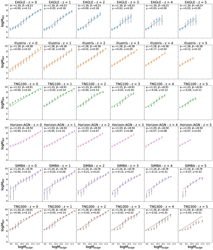
Figure 1: Variation of the BH mass with respect to galaxy bulge mass and variation in redshift using Eqn (29) for EAGLE, Illustris, TNG100, Horizon-AGN, SIMBA, and TNG300 simulations.

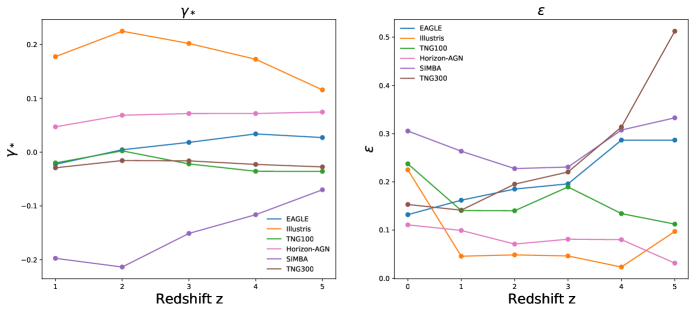
Figure 2: Variation of fitted $\gamma_{*}$ and $\epsilon$ values with redshift for the EAGLE, Illustris, TNG100, Horizon-AGN, SIMBA, and TNG300 simulations.

4 Analysis Setup

The characteristic spectrum is a function of nineteen parameters which can be estimated from astrophysical observables. These parameter are the five GSMF parameters $\Phi_{0},\Phi_{I},M_{0},\alpha_{0},\alpha_{I}$ , the four pair fraction parameters $f_{0},\alpha_{f},\beta_{f},\gamma_{f}$, the four merger timescale parameters $\tau_{0},\alpha_{\tau},\beta_{\tau},\gamma_{\tau}$, four BH-bulge mass parameters $\alpha_{*},\beta_{*},\gamma_{*},\epsilon$, and the two parameters $e_{0},\rho_{0}$ related to the binary GW emission which were defined in Eqn (10).

In order to find the redshift volume that PTA can probe for galaxy and SMBH mergers we consider $z_{m}$, which is the maximum redshift that is used to compute the volume, as an additional parameter to see the change in GWB characteristic strain if the volume is larger or smaller.

The GWB spectrum is computed from Eqn (15). The differences for six large-scale simulation data are shown in Figure 3 with the corresponding parameters given in Table 2.

The effect of each of these 20 astrophysical parameters on the GWB is shown in Figure 14.

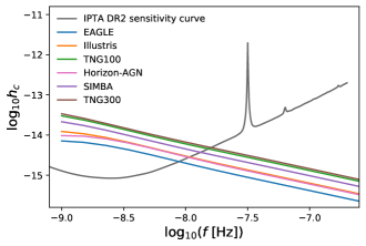
Figure 3: GWB characteristic strain values in the PTA range with the BH-bulge mass parameters for the EAGLE, Illustris, TNG100, Horizon-AGN, SIMBA, and TNG300 simulations. An analytic sensitivity curve from the IPTA DR2 is plotted to guide the eye.

4.1 Bayesian analysis

To the simulate a detection of the GWB at each frequency we assume a Gaussian distribution of central logarithmic amplitude $\log_{10}A_{\text{det}}(f)$ and width $\sigma_{\text{det}}(f)$ which are the detection measurement errors. With the GWB computed from a trial parameter set $\log_{10}A_{\rm trial}(f)$ the likelihood function can be written as

$$p_{det}(d\ |A_{\text{trial}}(f))\propto\exp\{\frac{-\big{(}\log_{10}A_{\text{trial}}(f)-\log_{10}A_{\text{det}}(f)\big{)}^{2}}{2\sigma_{\text{det}}(f)^{2}}\Bigg{\}}.$$ (30)

The Parallel Tempering Markov Chain Monte-Carlo (PTMCMC) Sampler (Ellis & van Haasteren, 2017) is used with $\sigma_{\rm det}=0.09$ for the Bayesian Analysis.

4.2 Prior choice

The prior for the BH-Bulge mass relation is constrained using all possible masses from the six different simulations for $z\leq 5$ to set the allowed range as shown in Figure 4 and the initial test values are given the Table 3. Only combinations of $\alpha_{*},\beta_{*}$,$\gamma_{*}$ and $z=(0,z_{max})$ that give a relation within the boundary are accepted.

Description	Parameter	range
BH-Bulge mass relation average slope	$\alpha_{*}$	[1,1.5]
BH-Bulge mass relation norm at $z=0$	$\beta_{*}$	[8,9]
BH-Bulge mass relation norm redshift evolution	$\gamma_{*}$	[-0.5,0.5]
BH-Bulge mass relation scatter	$\epsilon$	[0.05,0.5]
Maximmum redshift	$z_{m}$	[0.1,5]

Table 3: Prior choice for the black hole - bulge mass relation parameters including redshift variation.

The green lines in Figure 6 and Figure 7 show the boundary of Figure 4 as prior distributions within the values given in Table 3.

It is assumed that the redshift volume that PTAs are sensitive to is between 1.5 and 2.5. To study the effects of evolution with redshift and to test this assumption, we consider an extended range of $z_{m}\in[0.1,5]$, which includes the above range.

For the other parameters we adopt the same prior choice as in Chen et al. (2019).

Description	Parameter	range
GSMF norm	$\Phi_{0}$	[-3.4,-2.4]
GSMF norm redshift evolution	$\Phi_{I}$	[-0.6,0.2]
GSMF scaling mass	$\log_{10}M_{0}$	[11,11.5]
GSMF mass slope	$\alpha_{0}$	[-1.5,-1]
GSMF mass slope redshift evolution	$\alpha_{I}$	[-0.2,0.2]
pair fraction norm	$f_{0}$	[0.01,0.05]
pair fraction mass slope	$\alpha_{f}$	[-0.5,0.5]
pair fraction redshift slope	$\beta_{f}$	[0,2]
pair fraction mass ratio slope	$\gamma_{f}$	[-0.2,0.2]
merger time norm	$\tau_{0}$	[0.1,10.0]
merger time mass slope	$\alpha_{\tau}$	[-0.5,0.5]
merger time redshift slope	$\beta_{\tau}$	[-3,1]
merger time mass ratio slope	$\gamma_{\tau}$	[-0.2,0.2]
binary eccentricity	$e_{0}$	[0.01,0.99]
stellar density factor	$\log_{10}\rho_{0}$	[-2,2]

Table 4: Prior choice for the other astrophysical parameters.

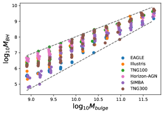
Figure 4: The allowed range for the BH mass at different bulge masses is denoted by the dashed lines. The BH masses of the EAGLE, Illustris, TNG100, Horizon-AGN, SIMBA, and TNG300 simulations for all redshift $z\leq 5$ are also shown.

4.3 GWB Simulations

Different values for the twenty parameters within the prior ranges give different GWB characteristic strain. Depending on the values of the twenty parameters, we can simulate a straight line or a curve bending down at low frequency for the GWB characteristic strain in the frequency range of $10^{-9}-10^{-6}$. In our model the line and curve spectra are associated with circular and eccentric SMBHB populations respectively. We created datasets for these two different types of spectrum for strain values of $0.5,1,2,3,4\times 10^{-15}$ at the reference frequency of $f=1/1$year ($f\approx 10^{-7.5}$ Hz) as shown in Figure 5. PTAs typically search at frequencies that are multiples of $1/T_{\rm span}$, where $T_{\rm span}$ is the total observation time span of the PTA dataset. For simplicity and computational efficiency, we use the five lowest bins with $T_{\rm span}=25$ years. The values of the parameters for the different spectra are in given Table 5.

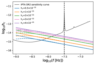
Figure 5: Different simulated GWB characteristic spectra in the PTA range. To guide the eye the analytic sensitivity curve from the IPTA DR2 and a vertical dashed line at reference frequency $f=1/1$year are also plotted.

Parameter	Line					Curve
$h_{c}$ at $f=\frac{1}{1\text{year}}$	$0.5\times 10^{-15}$	$1\times 10^{-15}$	$2\times 10^{-15}$	$3\times 10^{-15}$	$4\times 10^{-15}$	$0.5\times 10^{-15}$	$1\times 10^{-15}$	$2\times 10^{-15}$	$3\times 10^{-15}$	$4\times 10^{-15}$
$\Phi_{0}$	-2.9	-2.6	-2.9	-2.9	-2.9	-2.55	-2.5	-2.5	-2.5	-2.6
$\Phi_{I}$	-0.45	-0.45	-0.45	-0.45	-0.45	-0.45	-0.255	-0.1	0.08	.095
$M_{0}$	11.25	11.25	11.25	11.25	11.3	11.35	11.35	11.35	11.35	11.2
$\alpha_{0}$	-1.15	-1.15	-1.15	-1.15	-1.15	-1.1	-1.1	-1.1	-1.1	-1.1
$\alpha_{I}$	-0.1	-0.1	-0.1	-0.1	-0.1	-0.12	-0.12	-0.12	-0.12	-0.12
$f_{0}$	0.015	0.02	0.03	0.03	0.035	0.022	0.03	0.03	0.03	0.03
$\alpha_{f}$	0.3	0.3	0.3	0.3	0.3	-0.15	-0.15	-0.15	-0.15	-0.15
$\beta_{f}$	0.6	0.6	0.6	0.6	0.6	0.8	1.2	1.48	1.3	1.7
$\gamma_{f}$	0.1	0.1	0.1	0.1	0.1	0.1	0.1	0.1	0.1	0.1
$\tau_{0}$	2.	1.8	2.	2.	2.	0.8	0.8	0.8	0.8	0.8
$\alpha_{\tau}$	0.1	0.1	0.1	0.1	0.1	0.2	0.2	0.2	0.2	-0.2
$\beta_{\tau}$	-1.8	-2.	-2.1	-2.3	-2.5	-2.	-2.	-2.	-2.1	-2.1
$\gamma_{\tau}$	-0.1	-0.1	-0.1	-0.1	-0.1	-0.1	-0.1	-0.1	-0.1	0.1
$\alpha_{*}$	1.1	1.1	1.1	1.1	1.1	1.	1.	1.	1.	1.
$\beta_{*}$	8.5	8.5	8.65	8.8	8.8	8.0	8.0	8.0	8.0	8.1
$\gamma_{*}$	0.1	0.1	0.3	0.3	0.3	0.1	0.1	0.1	0.1	0.1
$\epsilon$	0.35	0.35	0.35	0.35	0.35	0.2	0.2	0.2	0.2	0.2
$e_{0}$	0.5	0.5	0.5	0.5	0.5	0.9	0.9	0.9	0.9	0.9
$\log_{10}\rho_{0}$	-0.1	-0.1	-0.1	-0.1	-0.1	-0.1	-0.1	-0.1	-0.1	-0.1
$z$	1.5	2.0	3.0	3.0	3.0	1.4	2.0	3.0	3.0	3.0

Table 5: Values of astrophysical parameters used for the different simulated detections shown in the Figure 5 .

5 Results

5.1 Constraints on astrophysical observables

5.1.1 BH-bulge mass relation

Simulated PTA GWB detections are used to perform the Bayesian analysis to find the posterior constraints on the astrophysical parameters in our model.

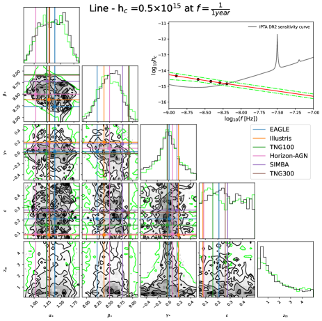
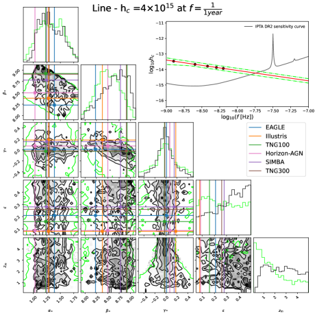
Figure 6: Posterior distributions of $\alpha_{*},\beta_{*},\gamma_{*}$, scatter $\varepsilon$ and maximum redshift $z_{m}$ for two different straight line characteristic strain spectra of $0.5$ and $4\times 10^{-15}$ at $f=1/1$year denoted by black lines are shown on the left and right panels respectively. The prior distributions are denoted by light green lines. The values of the parameters for the six large-scale cosmological simulation are also shown in the main figures. The top right inlay of both figures shows the corresponding characteristic spectrum with the allowed error range, where the 5 points denote the frequency bins of $1/25$year, $2/25$year, $3/25$year, $4/25$year and $5/25$year which are used for the Bayesian analysis. To guide the eye the IPTA DR2 sensitivty curve is also plotted.

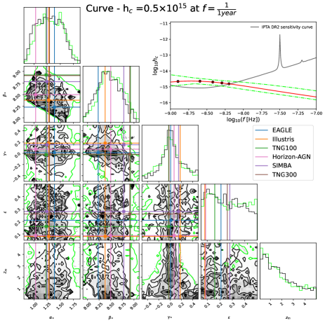
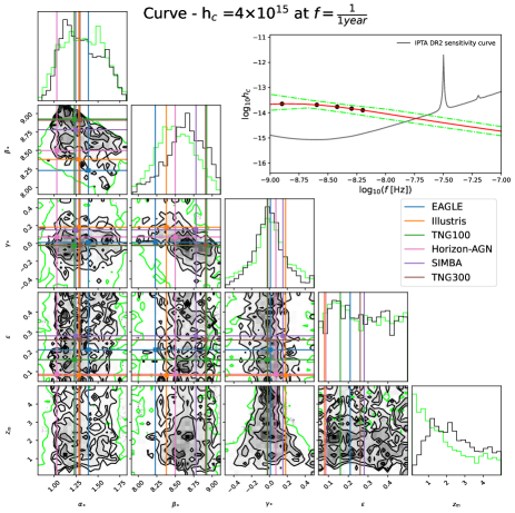
Figure 7: Same style as Figure 6, but for two different curved characteristic strain spectra of $0.5$ and $4\times 10^{-15}$ at $f=1/1$year.

We note that most of the other parameters are very similar to their priors, indicating that they are either already well constrained by other observations or they play only a mild role in the amplitude of the strain values. One exception is the merger time.

We can thus focus on the black hole - galaxy bulge mass redshift dependent relation parameters $\alpha_{*},\beta_{*},\varepsilon$ and $z$. Figure 6 and Figure 7 show their 2D and 1D posterior distributions for the cases of circular and eccentric populations respectively. We show only the cases for the smallest and largest amplitudes from our simulated detections. In the inlay figures we can see that the characteristic strains recovered from the posterior parameters fit well with the simulated detections.

First, looking at circular population in Figure 6, there is little difference between the priors (green) and the posteriors (black). All simulation fitted values lie within the allowed region. A detected amplitude of $h_{c}=0.5\times 10^{-15}$ provides little extra information. As the amplitude increases to $h_{c}=4\times 10^{-15}$, certain regions of the parameter space are ruled out. Noticeably in $\beta_{*}$ and $\varepsilon$, which both show a tendency for larger values. As high redshift black holes tend to be heavier, a trend for faraway SMBHBs also starts to emerge. The parameters of some simulations (like Horizon-AGN, Eagle and SIMBA) are outside the contour in higher characteristic spectrum.

Introducing a bend at the lowest frequencies from eccentric population of SMBHBs, shown in Figure 7, only marginally changes the findings from circular populations. The eccentricity and the environment of the black holes can only have an effect, if the bend is more prominent in the PTA frequency band.

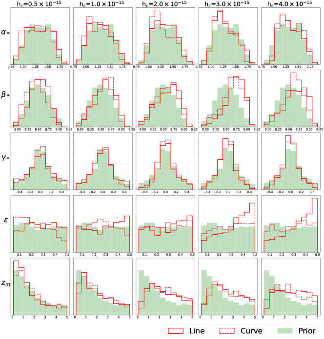
Figure 8: Distribution of all the BH-bulge mass parameters including redshift variation with the increase in characteristic strains values for both curved and straight line and spectra.

The evolution of the parameter constraints with amplitude can be found in Figure 8. As the characteristic strain amplitude becomes higher most parameters $\alpha_{*},\beta_{*},\varepsilon$ and $z$ prefer higher values and $\gamma_{*}$ becomes closer to zero. This suggests that a PTA detection can put constraints on the redshift evolution of the BH-bulge mass relation.

The corner plots for the complete twenty parameters with amplitudes $h_{c}=0.5\times 10^{-15},1\times 10^{-15},2\times 10^{-15},3\times 10^{-15},$ and $4\times 10^{-15}$ for both circular and eccentric population of SMBHBs are presented in Appendix B.

5.1.2 SMBHB merger rate

An interesting quantity that can be computed from our model is the merger rate of the SMBHBs from Eqn (16) given the constraints on the parameters from the simulated GWB detections. Following Chen et al. (2019), we first integrate over the mass ratio, leaving a merger rate by redshift and chirp mass. Next, we can integrate over the mass and redshift to get Figure 9 and Figure 10 showing $\differential n/\differential\mathcal{M}$ and $\differential n/\differential z$ respectively.

The merger rates with respect to the SMBHB mass in Figure 9 are very similar between the circular and eccentric populations at most investigated strain amplitudes. This indicates that environmental effects are not strongly covariant with the population properties. Only at the lowest amplitude $h=0.5\times 10^{-15}$ differences become noticeable with the eccentric population having a larger number of low mass binaries and the high mass drop-off at lower masses, compared to the circular population. This general trend persists through increasing amplitudes, but becomes less significant. In general, with larger amplitude the rate of massive binary mergers also grows. The median merger rate moves towards a drop-off at higher mass. Additionally, one can see an increase of the merger rate for smaller mass binaries in the 2-sigma range, especially in the circular population.

As we introduced the maximum redshift as a free parameter, the merger rates with respect to the redshift drop to zero at different maximum redshifts. This mimics the expectation that the GWB that PTAs are sensitive to will be dominated by closeby binaries. As such, we have binned the posterior samples by their maxmimum redshift. Within each bin we plot the merger rate within a common range of redshifts in Figure 10. E.g., in the left most column we selected all the posterior samples with a maximum redshift of $z<1$ and plot the integrated merger rate between 0.1 and 0.5.

In general, the median merger rate as a function of redshift is nearly constant across most redshifts, amplitudes and different populations. A small raise as the detected amplitude increases can be seen. The difference between the two populations is very small with the eccentric population requiring an overall larger number of mergers. As in the mass dependent merger rates, the main differences can be seen at the lowest amplitude. At $h=0.5\times 10^{-15}$ the drop of the lower bounds of the merger rate at high redshift is clearly visible. This is consistent with the prior assumption of a possible decreasing number of SMBHBs at high redshifts contributing to the GWB. Consequently, the number of samples for the highest maximum redshift is also low. If a detection favours high amplitudes, more binaries even at large distances are required to produce the GWB. This can be seen most prominently in the rightmost column in Figure 10, where the 2-sigma lower bound drop of the merger rate moves from $z\approx 1$ to $z\approx 4$.

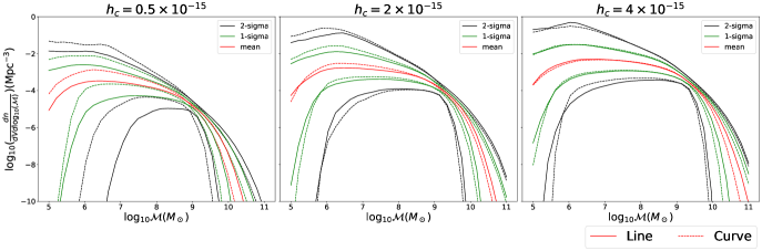
Figure 9: Merger rates with respect to the chirp mass of the SMBHB for increasing characteristic strain values for both curved and straight line spectra.

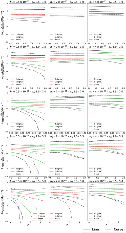
Figure 10: Merger rates with respect to redshift for increasing characteristic strains values of both curved and straight line spectra.

5.2 Constraints from Illustris and SIMBA

By fixing the BH-bulge mass parameters to the best fit values from the Illustris and SIMBA simulations given in Table 2, we can see how the constrains on the other parameters are affected. These two cosmological simulations are chosen since Illustris shows positive while SIMBA shows negative evolution of the SMBH mass with redshift, and thus are the extreme two cases in these six large-scale cosmological simulations. The distribution of all the astrophysical parameters for both curved and straight line characteristic spectra of the GWB and with fixed BH-bulge mass parameter values to match Illustris and SIMBA are given in the Figure 11, where Illustris is shown in blue, SIMBA in pink and the prior of the parameters in the green shaded regions.

The evolution of the pair fraction parameters displays similarities in both the curved and straight line characteristic spectra for different amplitudes in Illustris and SIMBA, with some minor differences. At a characteristic spectrum value of $h_{c}=0.5\times 10^{-15}$, both Illustris and SIMBA exhibit posteriors similar to the prior for the pair fraction norm $f_{0}$. Only the curved spectrum in Illustris exhibits a trend towards larger values, with the Illustris simulation favouring larger values of $f_{0}$ more significantly than SIMBA at all amplitudes. As the strain value increases, both Illustris and SIMBA start to display posterior distributions that prefer larger values of $f_{0}$.

The pair fraction mass slope $\alpha_{f}$ in Illustris shows a preference for low values at $h_{c}=0.5\times 10^{-15}$, followed by no preference at $h_{c}=2\times 10^{-15}$, and then higher values at $h_{c}=4\times 10^{-15}$ for the curved strain. The straight line spectrum in Illustris begins with a distribution similar to the prior for $\alpha_{f}$ at $0.5\times 10^{-15}$ and tends towards higher values with larger strains. The SIMBA posterior distributions exhibit similar trends as their Illustris counterparts, but at larger strain, they display more uniform posteriors compared to the skewed ones in Illustris. The posterior distributions of the pair fraction redshift slope $\beta_{f}$ for both the curved and straight line spectra exhibit similar evolution with amplitude as in the case of $\alpha_{f}$ for Illustris and SIMBA. In conclusion, the pair fraction increases with larger amplitudes for both circular and eccentric populations. More massive and distant galaxy pairs are required to produce the gravitational wave background at higher strains. Illustris tends to require more pairs than SIMBA for the same amplitude.

The curved characteristic spectrum with a value of $h_{c}=0.5\times 10^{-15}$ in SIMBA reveals a correlation between higher posterior values of $\alpha_{\tau}$ and $\beta_{\tau}$ and higher values of eccentricity $e_{0}$ and $\rho_{0}$. On the other hand, Illustris shows a lower posterior value for $\alpha_{\tau}$ and $\beta_{\tau}$ with higher values of $e_{0}$ and $\rho_{0}$. An increase in the characteristic spectrum values of the curved line leads to slightly higher values of $e_{0}$ and $\rho_{0}$, but prefers lower values of $\alpha_{\tau}$ and $\beta_{\tau}$ in both Illustris and SIMBA. This indicates that the variation of $\gamma_{*}$ influences $\alpha_{\tau}$ at lower characteristic spectrum values. A similar effect is observed for $\beta_{\tau}$ on the straight line characteristic spectrum values, despite a uniform posterior of $e_{0}$ and $\rho_{0}$. With higher straight line characteristic spectrum values, the trend in $\alpha_{\tau}$ is similar to the curved line case, but instead of a higher value of $\alpha_{\tau}$ at lower characteristic spectrum values, a uniform posterior distribution is observed, similar to $e_{0}$ and $\rho_{0}$.

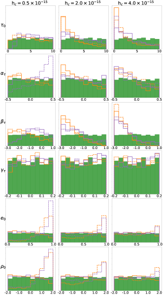
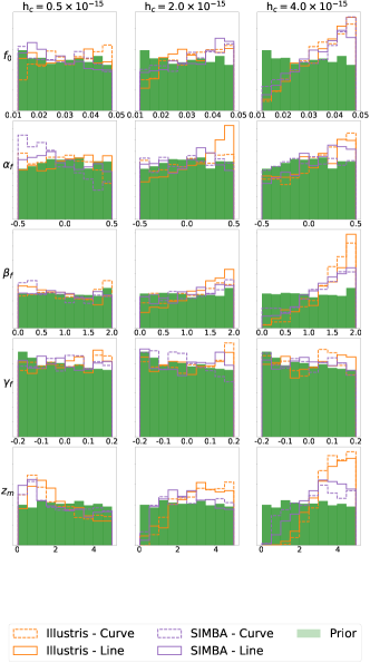
Figure 11: Distributions of all the astrophysical parameters for both curved and straight line characteristic spectra by fixing the BH-bulge mass parameter values to Illustris and SIMBA.

The corner plots for the sixteen parameters with amplitudes $h_{c}=0.5\times 10^{-15},2\times 10^{-15},$ and $4\times 10^{-15}$ for both circular and eccentric population of SMBHBs using the fitted BH-bulge mass parameters from Illustris and SIMBA are presented in Appendix C.

It is interesting to look at $\differential n/\differential\mathcal{M}$ and $\differential n/\differential z$ as in the previous section for the Illustris and SIMBA simulations as shown in Figure 12 and Figure 13. The most prominent feature of $\differential n/\differential\mathcal{M}$ in Figure 12 is a shift towards larger mass from Illustris to SIMBA for the same GWB strain. This is consistent with the prediction that SIMBA produces lower mass binaries than Illustris and thus need more binaries to match the emitted GWB strain. The free parameters are adjusted to get same amplitude as explained above from Figure 11. The other feature that is visible from Figure 12 is the variation between circular and eccentric binaries producing a straight and curved GWB strain spectrum respectively. There is no difference in the median of the merger rates with respect to the SMBHB mass in Illustris for the circular and eccentric binaries with same amplitude, however we can see small differences at the lower 2-sigma boundaries. SIMBA clearly shows a slight variation in binary chirp mass between circular and eccentric binaries.

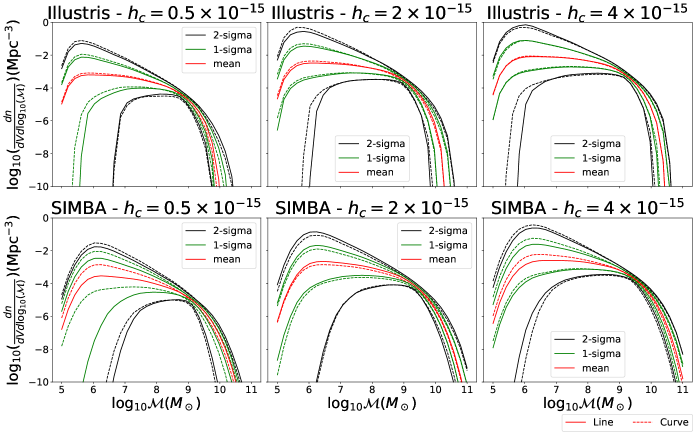
Figure 12: Merger rates with respect to the chirp mass of the SMBHB using fits to Illustris and SIMBA for increasing characteristic strains values for both curved and straight line spectra.

The merger rate with respect to the redshift is shown in Figure 13 for Illustris and SIMBA with the panels defined in the same way as in the previous section and Figure 10. An important feature here is that no GWB strain amplitude of $h_{c}=4\times 10^{-15}$ can be obtained from a circular population of binaries with redshifts $z<1.0$ and only very few eccentric populations could produce such amplitude in our sampling. Within the small number statistical uncertainties it seems that such a large amplitude is rarely achieved by any simulation within $z<1.0$. While in general the results from Illustris and SIMBA in Figure 13 are very similar to those in Figure 10, the merger rates for Illustris become nearly constant across all redshifts at amplitude of $h_{c}=2\times 10^{-15}$ already.

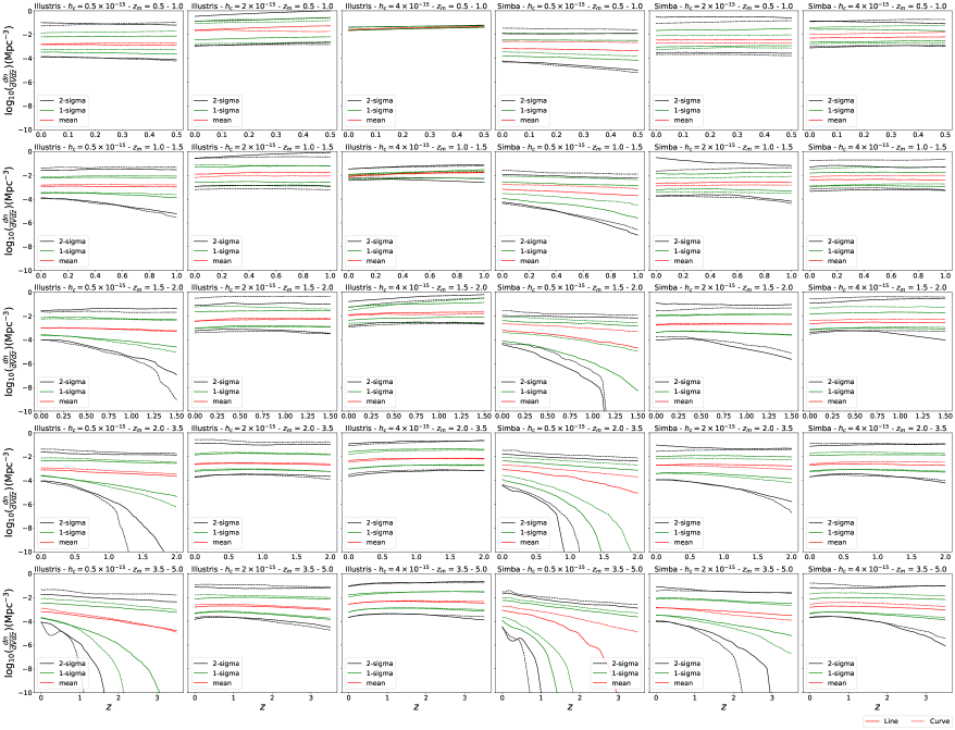
Figure 13: Merger rates with respect to redshift using fits to Illustris and SIMBA for increasing characteristic strain values for both curved and straight line spectra.

6 Discussion and conclusions

The analytical astrophysical model presented in this work describes the intensity of the gravitational wave background as a function of the frequency. The focus was on the redshift dependent BH-bulge mass relation. By understanding the processes and relationships concerning the formation and co-evolution of galaxies and their central black holes, we have used theoretical and analytical expressions in order to refine current astrophysical models. This allowed us to compare the predictions of this model with the constraints from PTA observations.

Large-scale cosmological simulations help us to study the evolution of the Universe since observational unbiased data is hard to produce. Having a good formalism of the evolution of central black hole of galaxies and galaxy mergers is important to understand many astrophysical properties of the Universe. A GWB detection with PTA will provide additional observational knowledge. We proposed a formalism for the redshift dependence of the BH-bulge mass relation for $z<5$, and found $\gamma_{*}$ to be more restricted at higher redshifts. We find the tightest constraints for $\beta_{*}$ from a GWB detection in the PTA range.

Varying the maximum redshift parameter in the model seen in Figure 14 shows that the dominant fraction of the SMBHB population can be found withing $z_{m}\sim 1.5-2.5$ with the SMBHBs at higher redshifts only contributing a small, but not negligible, amount to the GWB. The study of higher redshift galaxies will be useful for the evolution of BH-bulge mass of galaxies with redshift. There still are observational difficulties for higher redshift galaxies compared to quasars.

The redshift dependent BH-bulge mass relation proposed by Venemans et al. (2016) gives higher scattering values for the different simulations we have used. Our proposed relation gives more consistent results with lower scattering values for those simulations. However, (Graham, 2012) propose a double power law for the redshift independent BH-bulge mass relation of galaxies using observational data. Further studies to find and test the optimal shape of a redshift dependent BH-bulge mass relation are required. Another interesting area for further improvement of the model is the galaxy stellar-bulge mass relation. The phenomenological stellar-bulge mass relation we have used is more suitable for elliptical and spheroidal galaxies, so a relation containing spiral galaxies including a degree of the spirality will be ideal to study a wide range of galaxies and their central black holes.

Appendix A GWB characteristic spectra from variations of the astrophysical parameters

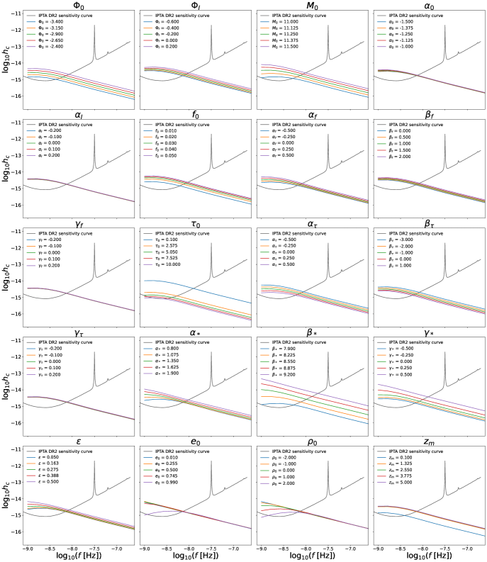
Figure 14: Effect on the GWB spectrum from variations of each of the twenty astrophysical parameters within the range given in Table 3 and Table 4. The default values are set for the parameters as: $\Phi_{0}=-2.6,\Phi_{I}=-0.45,M_{0}=11.25,\alpha_{0}=-1.15,\alpha_{I}=-0.1,f_{0}=0.02,\alpha_{f}=0.1,\beta_{f}=0.8,\gamma_{f}=0.1,\tau_{0}=0.8,\alpha_{\tau}=-0.1,\beta_{\tau}=-2.,\gamma_{\tau}=-0.1,\alpha_{*}=1.1,\beta_{*}=8.2,\gamma_{*}=-0.2,\epsilon=0.3,e_{0}=0.9,\log_{10}\rho_{0}=0.1,z=2.0$.

Appendix B Full corner plots of the twenty parameters

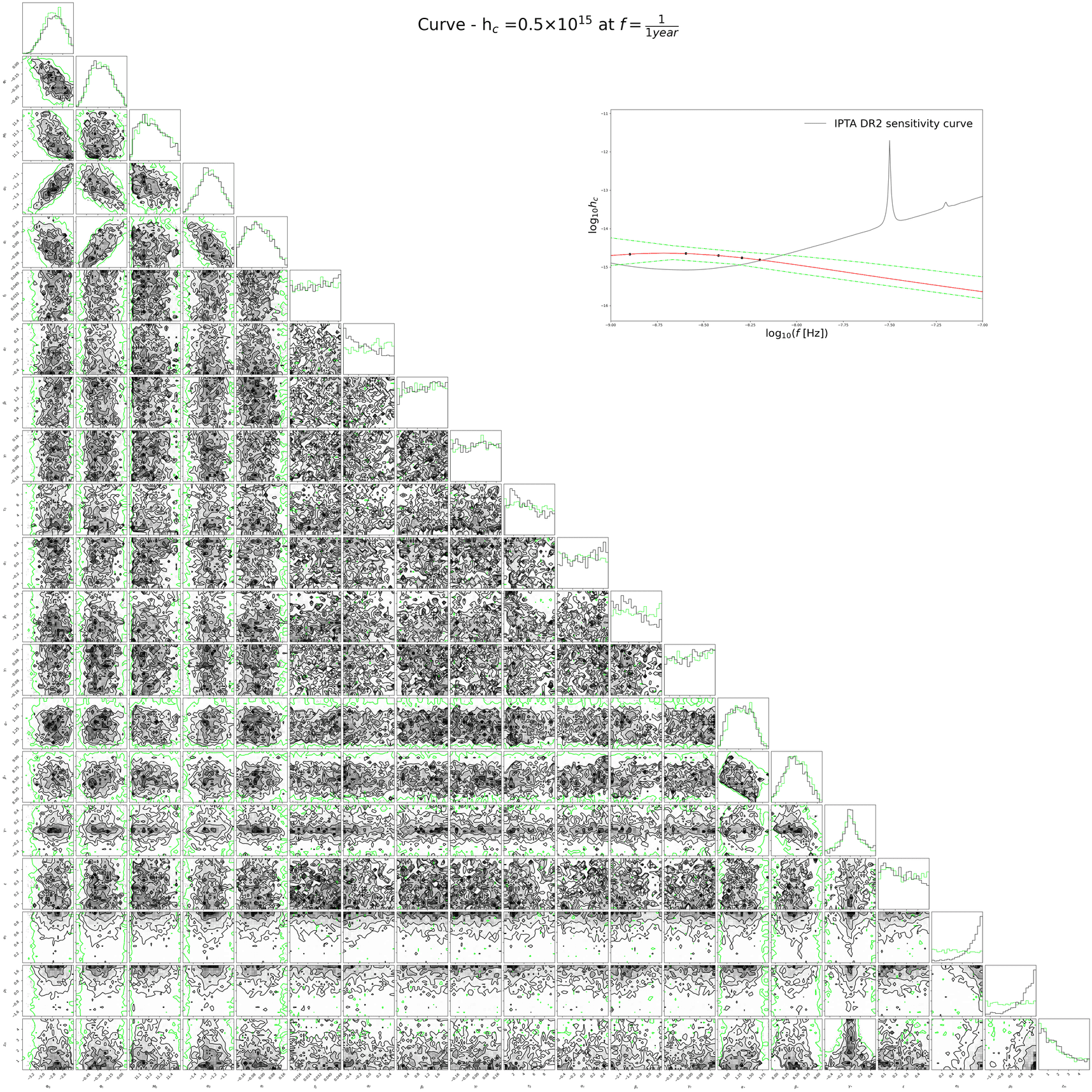
Figure 15: Corner plot of the twenty parameters for curved line characteristic strain spectrum of $h_{c}=0.5\times 10^{-15}$ is denoted by the black lines. The prior distribution is denoted by the light green lines. Top right of both figures show the characteristic spectrum of the corner plot with the allowed error range, where the 5 points denote the frequency bins of $1/25$year, $2/25$year, $3/25$year, $4/25$year and $5/25$year which is used for the Bayesian analysis to create the posterior distribution. Also just to guide the eye, the IPTA DR2 Sensitivty curve is plotted in it.

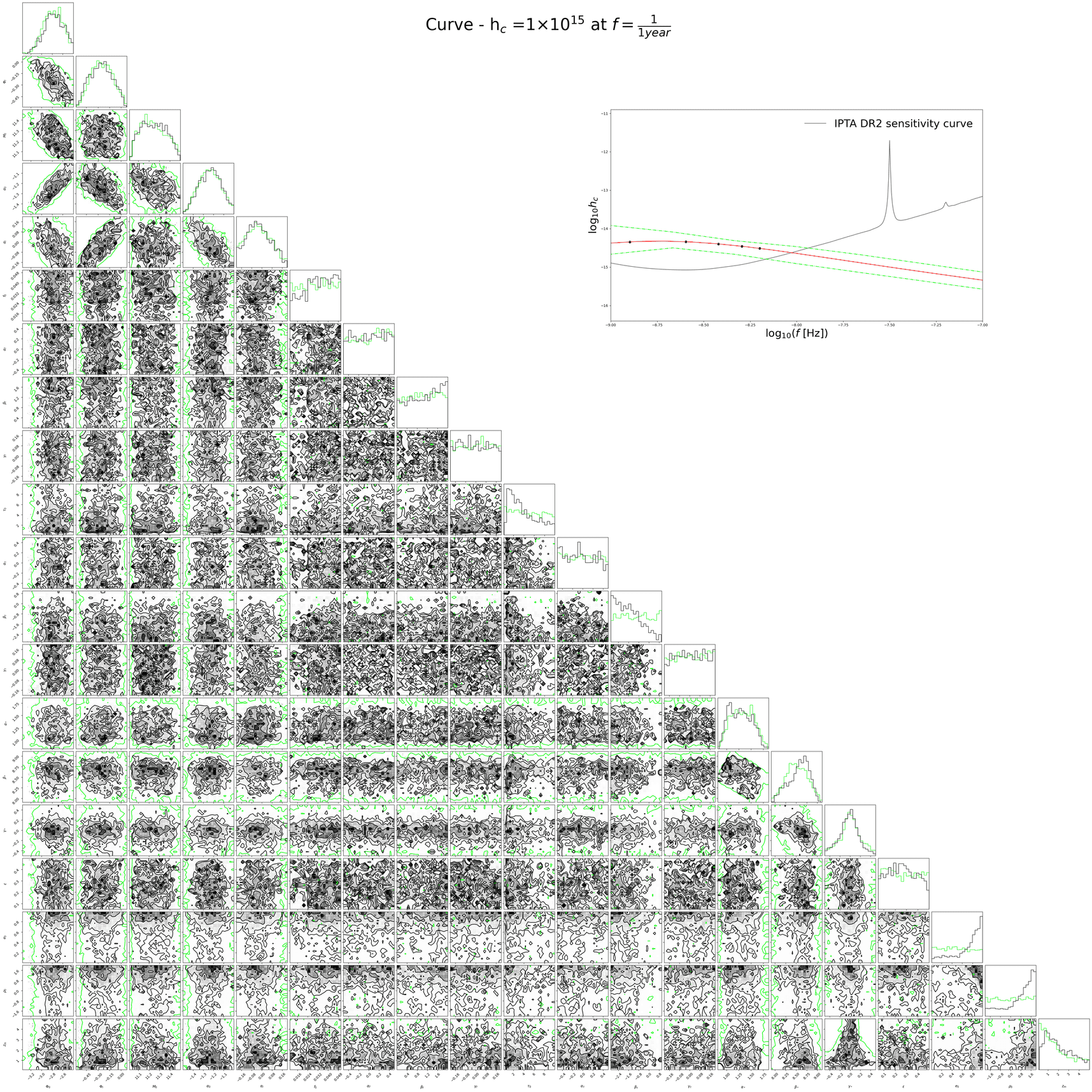
Figure 16: Corner plot of the twenty parameters for curved line characteristic strain spectrum of $h_{c}=1\times 10^{-15}$. Top right of both figures show the characteristic spectrum of the corner plot with the allowed error range, where the 5 points denote the frequency bins of $1/25$year, $2/25$year, $3/25$year, $4/25$year and $5/25$year which is used for the Bayesian analysis to create the posterior distribution. Also just to guide the eye, the IPTA DR2 Sensitivty curve is plotted in it.

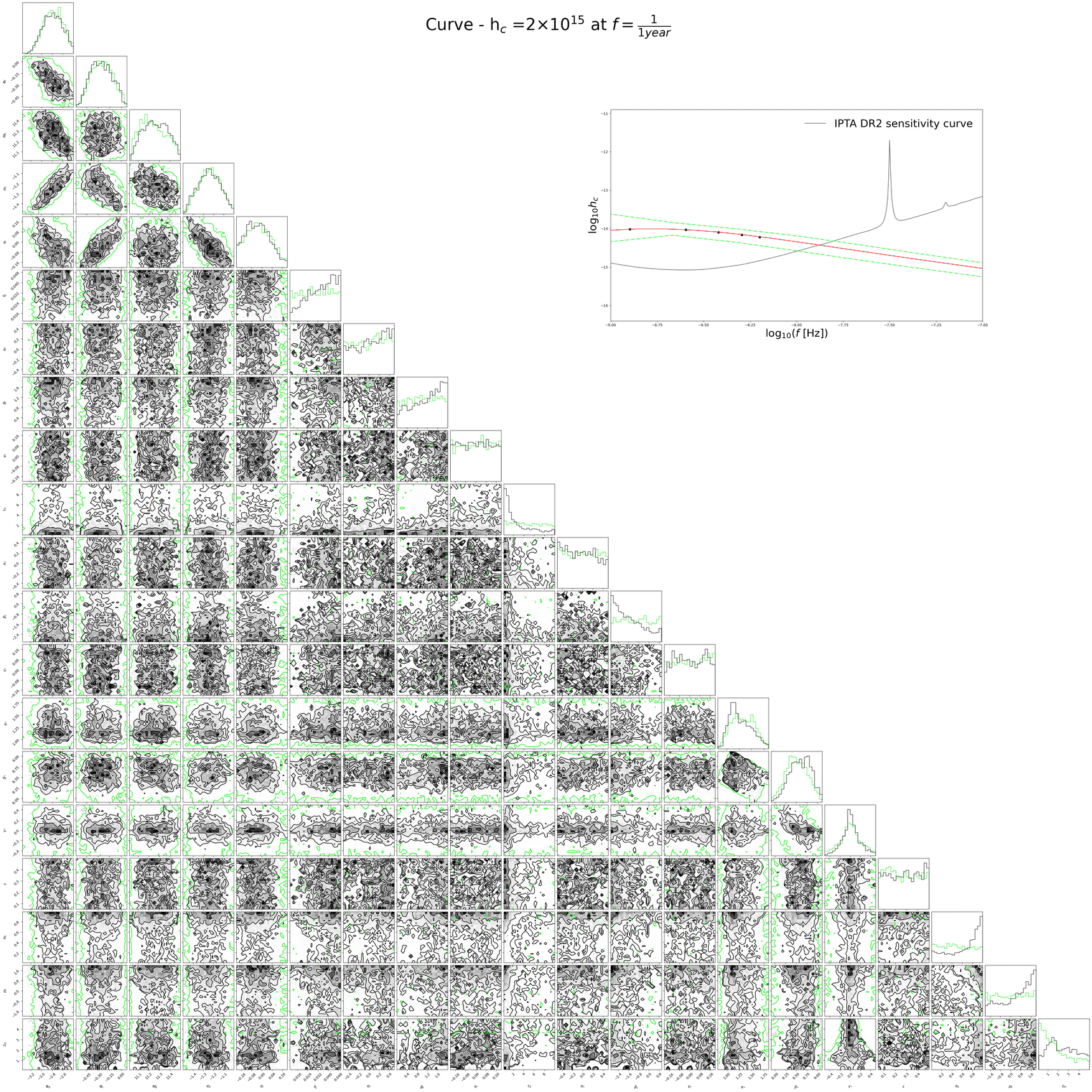
Figure 17: Corner plot of the twenty parameters for curved line characteristic strain spectrum of $h_{c}=2\times 10^{-15}$ is denoted by the black lines. The prior distribution is denoted by the light green lines. Top right of both figures show the characteristic spectrum of the corner plot with the allowed error range, where the 5 points denote the frequency bins of $1/25$year, $2/25$year, $3/25$year, $4/25$year and $5/25$year which is used for the Bayesian analysis to create the posterior distribution. Also just to guide the eye, the IPTA DR2 Sensitivty curve is plotted in it.

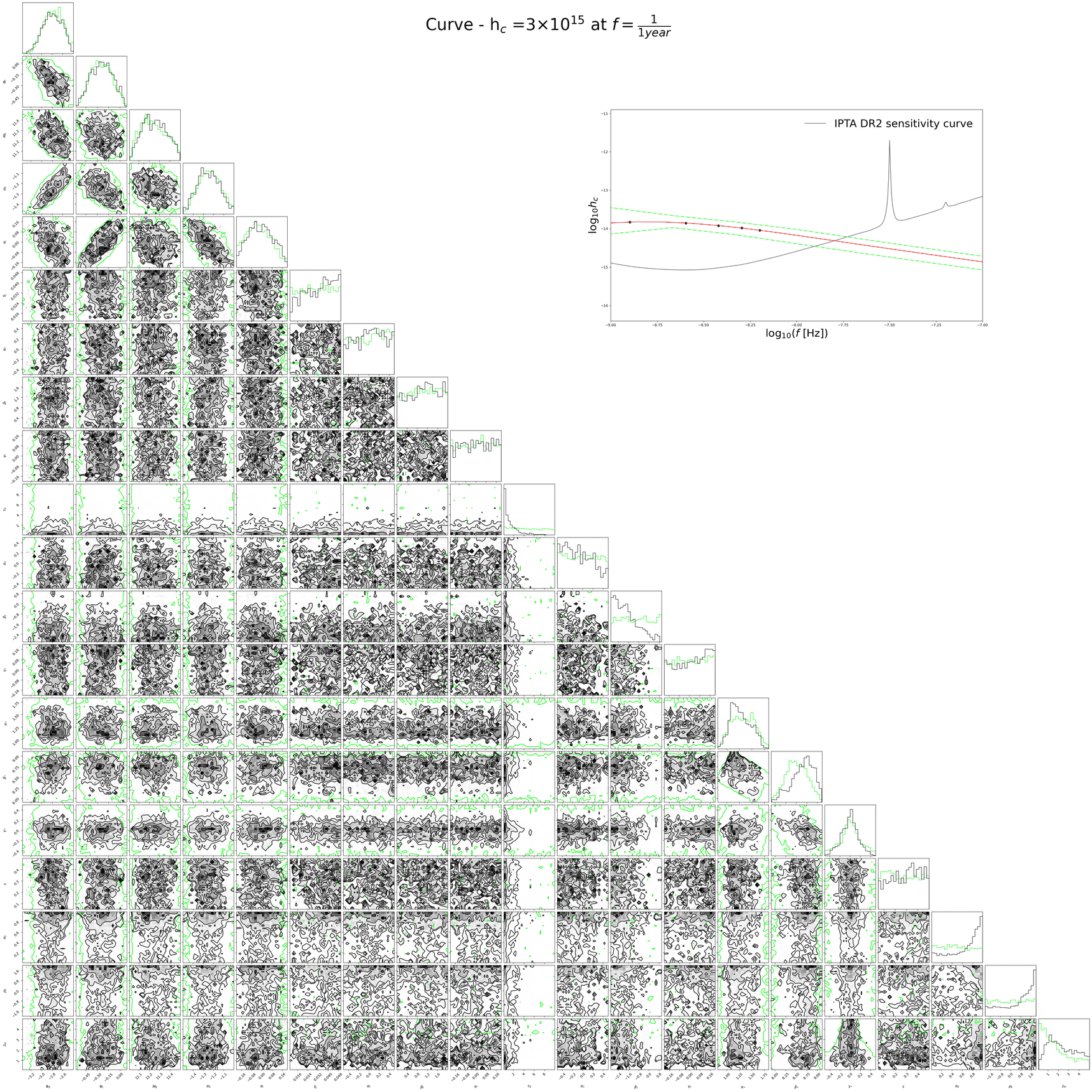
Figure 18: Corner plot of the twenty parameters for curved line characteristic strain spectrum of $h_{c}=3\times 10^{-15}$ is denoted by the black lines. The prior distribution is denoted by the light green lines. Top right of both figures show the characteristic spectrum of the corner plot with the allowed error range, where the 5 points denote the frequency bins of $1/25$year, $2/25$year, $3/25$year, $4/25$year and $5/25$year which is used for the Bayesian analysis to create the posterior distribution. Also just to guide the eye, the IPTA DR2 Sensitivty curve is plotted in it.

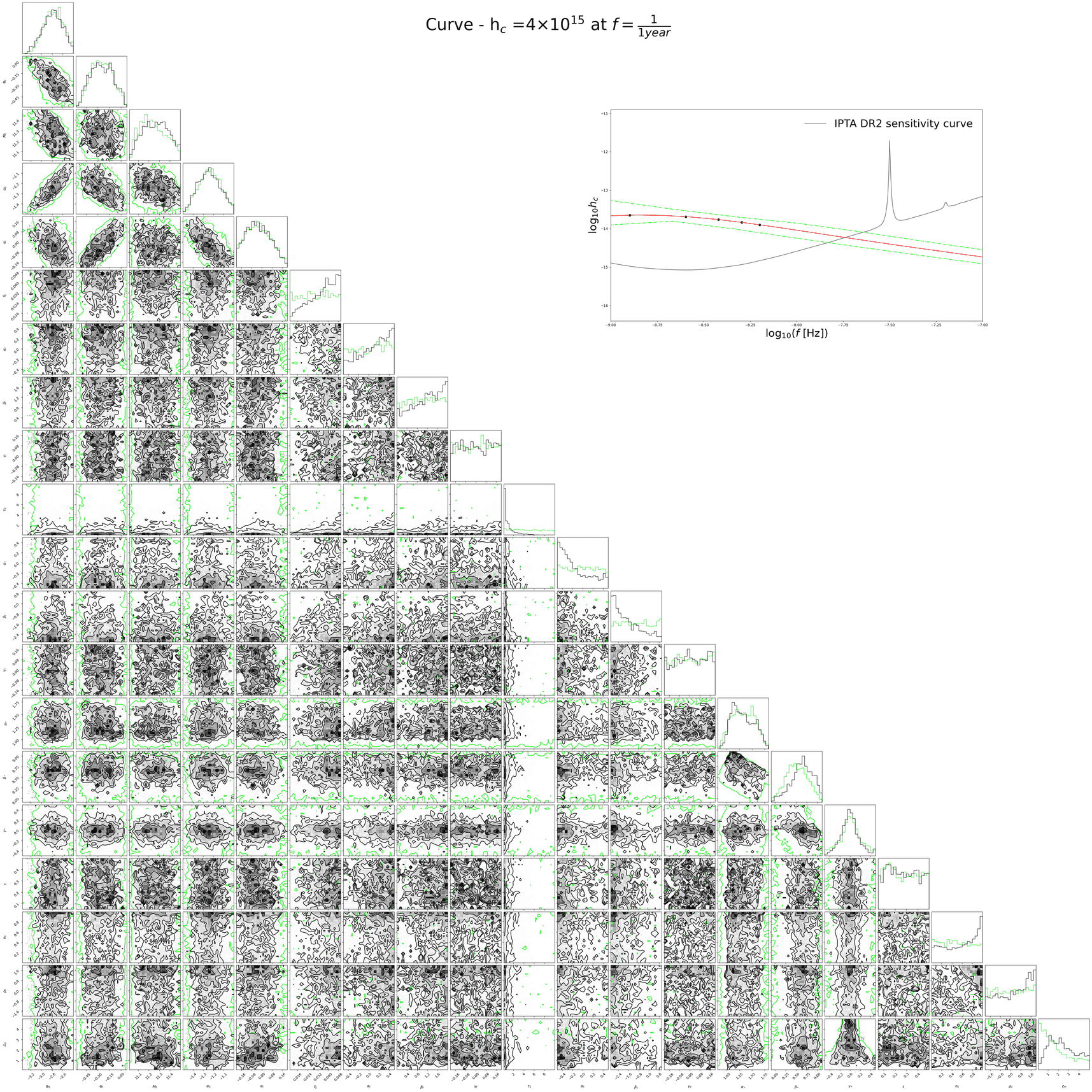
Figure 19: Corner plot of the twenty parameters for curved line characteristic strain spectrum of $h_{c}=4\times 10^{-15}$ is denoted by the black lines. The prior distribution is denoted by the light green lines. Top right of both figures show the characteristic spectrum of the corner plot with the allowed error range, where the 5 points denote the frequency bins of $1/25$year, $2/25$year, $3/25$year, $4/25$year and $5/25$year which is used for the Bayesian analysis to create the posterior distribution. Also just to guide the eye, the IPTA DR2 Sensitivty curve is plotted in it.

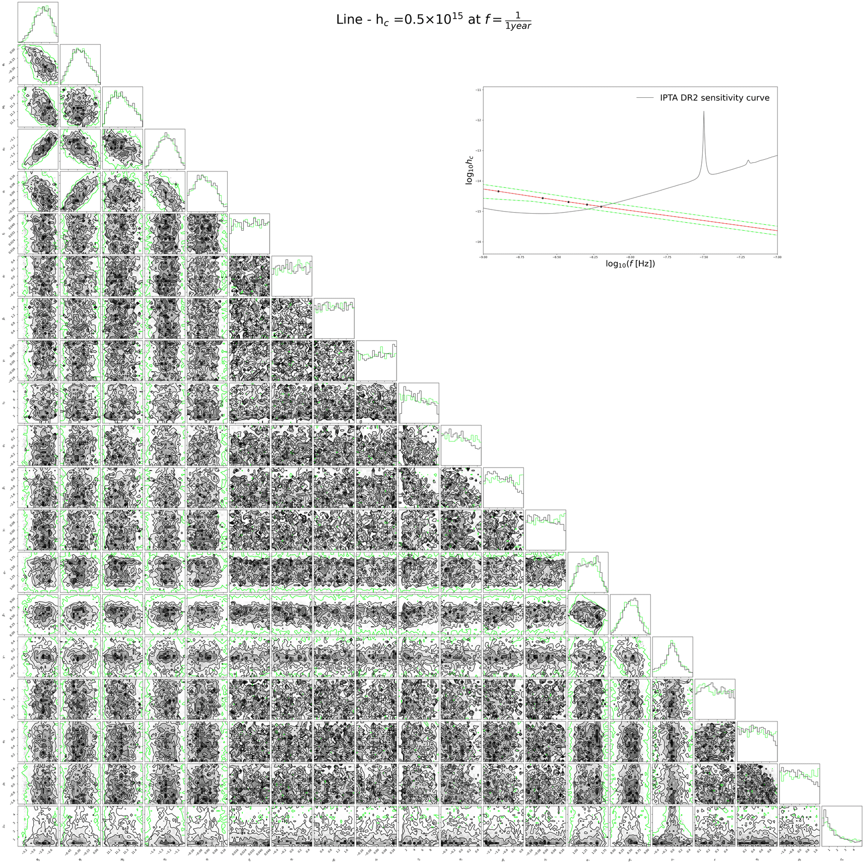
Figure 20: Corner plot of the twenty parameters for straight line characteristic strain spectrum of $h_{c}=0.5\times 10^{-15}$ is denoted by the black lines. The prior distribution is denoted by the light green lines. Top right of both figures show the characteristic spectrum of the corner plot with the allowed error range, where the 5 points denote the frequency bins of $1/25$year, $2/25$year, $3/25$year, $4/25$year and $5/25$year which is used for the Bayesian analysis to create the posterior distribution. Also just to guide the eye, the IPTA DR2 Sensitivty curve is plotted in it.

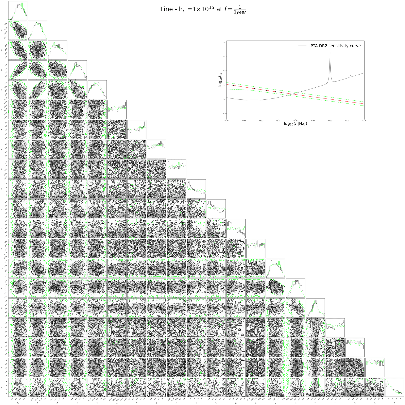
Figure 21: Corner plot of the twenty parameters for straight line characteristic strain spectrum of $h_{c}=1\times 10^{-15}$ is denoted by the black lines. The prior distribution is denoted by the light green lines. Top right of both figures show the characteristic spectrum of the corner plot with the allowed error range, where the 5 points denote the frequency bins of $1/25$year, $2/25$year, $3/25$year, $4/25$year and $5/25$year which is used for the Bayesian analysis to create the posterior distribution. Also just to guide the eye, the IPTA DR2 Sensitivty curve is plotted in it.

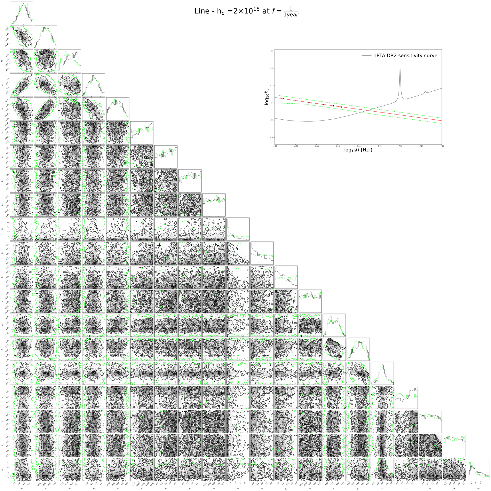
Figure 22: Corner plot of the twenty parameters for straight line characteristic strain spectrum of $h_{c}=2\times 10^{-15}$ is denoted by the black lines. The prior distribution is denoted by the light green lines. Top right of both figures show the characteristic spectrum of the corner plot with the allowed error range, where the 5 points denote the frequency bins of $1/25$year, $2/25$year, $3/25$year, $4/25$year and $5/25$year which is used for the Bayesian analysis to create the posterior distribution. Also just to guide the eye, the IPTA DR2 Sensitivty curve is plotted in it.

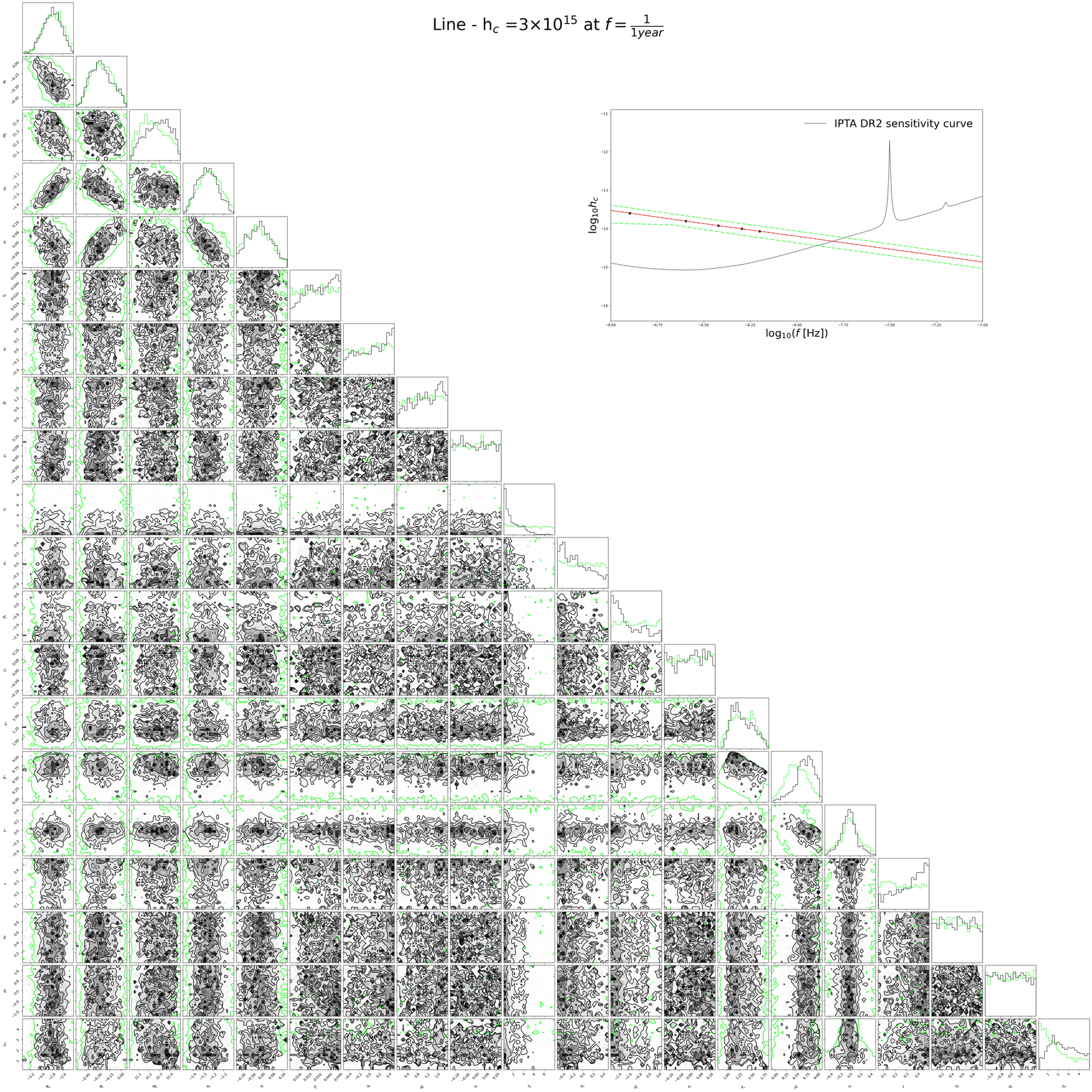
Figure 23: Corner plot of the twenty parameters for straight line characteristic strain spectrum of $h_{c}=3\times 10^{-15}$ is denoted by the black lines. The prior distribution is denoted by the light green lines. Top right of both figures show the characteristic spectrum of the corner plot with the allowed error range, where the 5 points denote the frequency bins of $1/25$year, $2/25$year, $3/25$year, $4/25$year and $5/25$year which is used for the Bayesian analysis to create the posterior distribution. Also just to guide the eye, the IPTA DR2 Sensitivty curve is plotted in it.

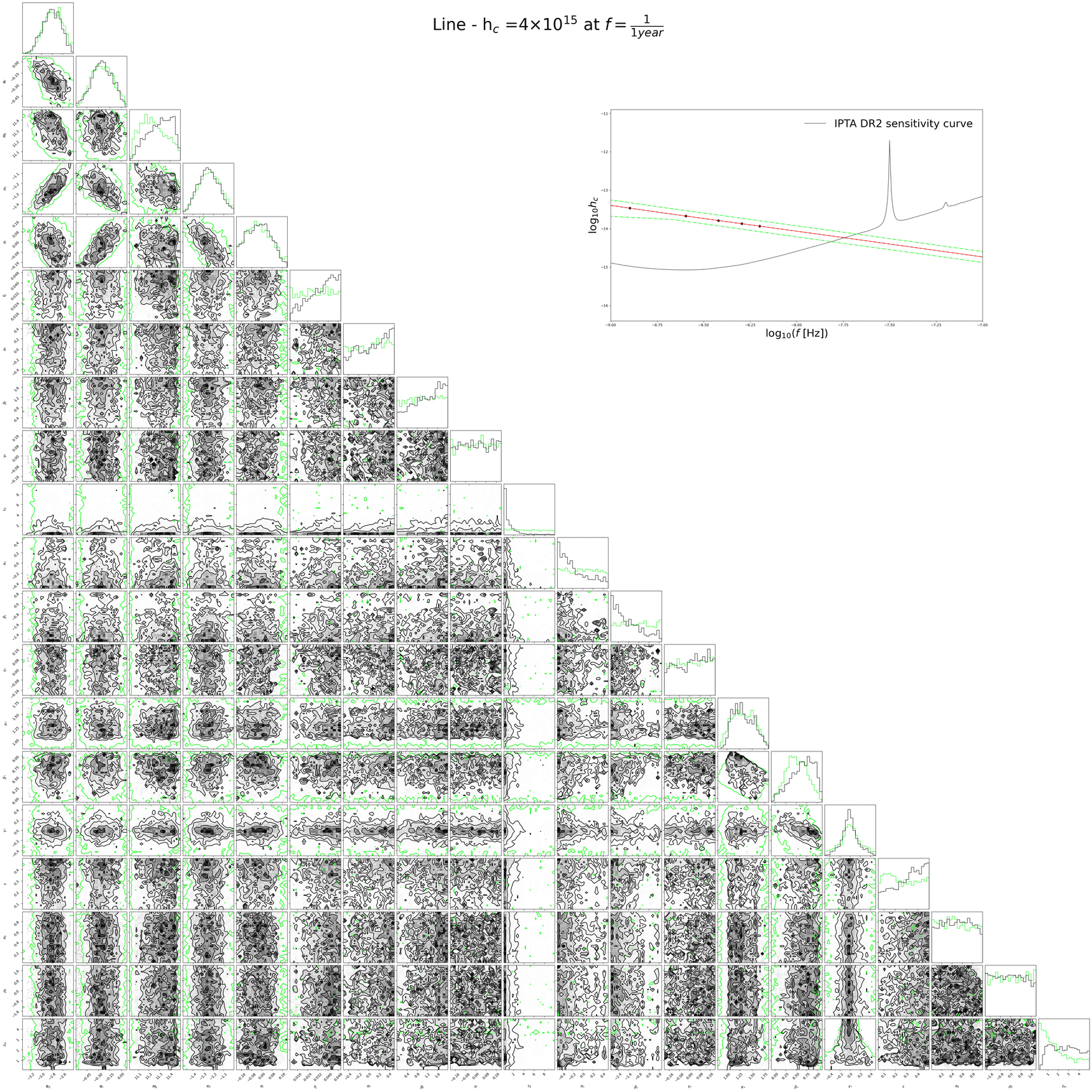
Figure 24: Corner plot of the twenty parameters for straight line characteristic strain spectrum of $h_{c}=4\times 10^{-15}$ is denoted by the black lines. The prior distribution is denoted by the light green lines. Top right of both figures show the characteristic spectrum of the corner plot with the allowed error range, where the 5 points denote the frequency bins of $1/25$year, $2/25$year, $3/25$year, $4/25$year and $5/25$year which is used for the Bayesian analysis to create the posterior distribution. Also just to guide the eye, the IPTA DR2 Sensitivty curve is plotted in it.

Appendix C Full corner plots of the sixteen parameters for Illustris and SIMBA

Figure 25: Corner plot of the sixteen parameters for curved line characteristic strain spectrum of $h_{c}=0.5\times 10^{-15}$ with black hole-bulge parameter of Illustris is denoted by the black lines. The prior distribution is denoted by the light green lines. Top right of both figures show the characteristic spectrum of the corner plot with the allowed error range, where the 5 points denote the frequency bins of $1/25$year, $2/25$year, $3/25$year, $4/25$year and $5/25$year which is used for the Bayesian analysis to create the posterior distribution. Also just to guide the eye, the IPTA DR2 Sensitivty curve is plotted in it.

Figure 26: Corner plot of the sixteen parameters for curved line characteristic strain spectrum of $h_{c}=2\times 10^{-15}$ with black hole-bulge parameter of Illustris is denoted by the black lines. The prior distribution is denoted by the light green lines. Top right of both figures show the characteristic spectrum of the corner plot with the allowed error range, where the 5 points denote the frequency bins of $1/25$year, $2/25$year, $3/25$year, $4/25$year and $5/25$year which is used for the Bayesian analysis to create the posterior distribution. Also just to guide the eye, the IPTA DR2 Sensitivty curve is plotted in it.

Figure 27: Corner plot of the sixteen parameters for curved line characteristic strain spectrum of $h_{c}=4\times 10^{-15}$ with black hole-bulge parameter of Illustris is denoted by the black lines. The prior distribution is denoted by the light green lines. Top right of both figures show the characteristic spectrum of the corner plot with the allowed error range, where the 5 points denote the frequency bins of $1/25$year, $2/25$year, $3/25$year, $4/25$year and $5/25$year which is used for the Bayesian analysis to create the posterior distribution. Also just to guide the eye, the IPTA DR2 Sensitivty curve is plotted in it.

Figure 28: Corner plot of the sixteen parameters for straight line characteristic strain spectrum of $h_{c}=0.5\times 10^{-15}$ with black hole-bulge parameter of Illustris is denoted by the black lines. The prior distribution is denoted by the light green lines. Top right of both figures show the characteristic spectrum of the corner plot with the allowed error range, where the 5 points denote the frequency bins of $1/25$year, $2/25$year, $3/25$year, $4/25$year and $5/25$year which is used for the Bayesian analysis to create the posterior distribution. Also just to guide the eye, the IPTA DR2 Sensitivty curve is plotted in it.

Figure 29: Corner plot of the sixteen parameters for straight line characteristic strain spectrum of $h_{c}=2\times 10^{-15}$ with black hole-bulge parameter of Illustris is denoted by the black lines. The prior distribution is denoted by the light green lines. Top right of both figures show the characteristic spectrum of the corner plot with the allowed error range, where the 5 points denote the frequency bins of $1/25$year, $2/25$year, $3/25$year, $4/25$year and $5/25$year which is used for the Bayesian analysis to create the posterior distribution. Also just to guide the eye, the IPTA DR2 Sensitivty curve is plotted in it.

Figure 30: Corner plot of the sixteen parameters for straight line characteristic strain spectrum of $h_{c}=4\times 10^{-15}$ with black hole-bulge parameter of Illustris is denoted by the black lines. The prior distribution is denoted by the light green lines. Top right of both figures show the characteristic spectrum of the corner plot with the allowed error range, where the 5 points denote the frequency bins of $1/25$year, $2/25$year, $3/25$year, $4/25$year and $5/25$year which is used for the Bayesian analysis to create the posterior distribution. Also just to guide the eye, the IPTA DR2 Sensitivty curve is plotted in it.

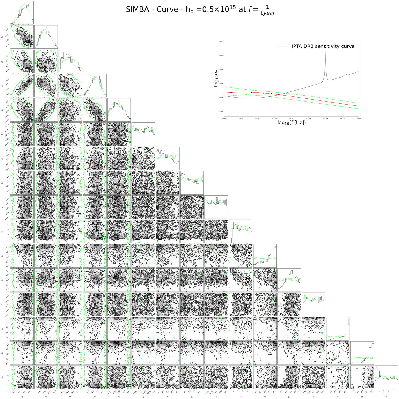
Figure 31: Corner plot of the sixteen parameters for curved line characteristic strain spectrum of $h_{c}=0.5\times 10^{-15}$ with black hole-bulge parameter of SIMBA is denoted by the black lines. The prior distribution is denoted by the light green lines. Top right of both figures show the characteristic spectrum of the corner plot with the allowed error range, where the 5 points denote the frequency bins of $1/25$year, $2/25$year, $3/25$year, $4/25$year and $5/25$year which is used for the Bayesian analysis to create the posterior distribution. Also just to guide the eye, the IPTA DR2 Sensitivty curve is plotted in it.

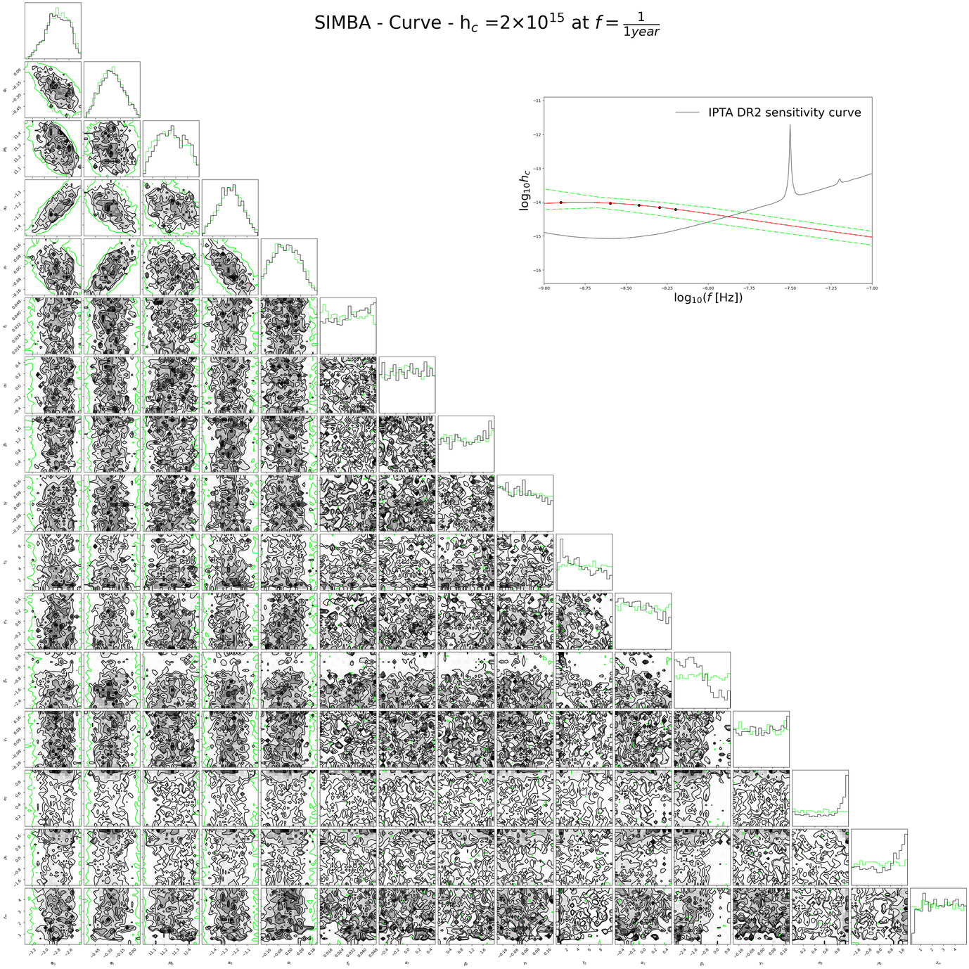
Figure 32: Corner plot of the sixteen parameters for curved line characteristic strain spectrum of $h_{c}=2\times 10^{-15}$ with black hole-bulge parameter of SIMBA is denoted by the black lines. The prior distribution is denoted by the light green lines. Top right of both figures show the characteristic spectrum of the corner plot with the allowed error range, where the 5 points denote the frequency bins of $1/25$year, $2/25$year, $3/25$year, $4/25$year and $5/25$year which is used for the Bayesian analysis to create the posterior distribution. Also just to guide the eye, the IPTA DR2 Sensitivty curve is plotted in it.

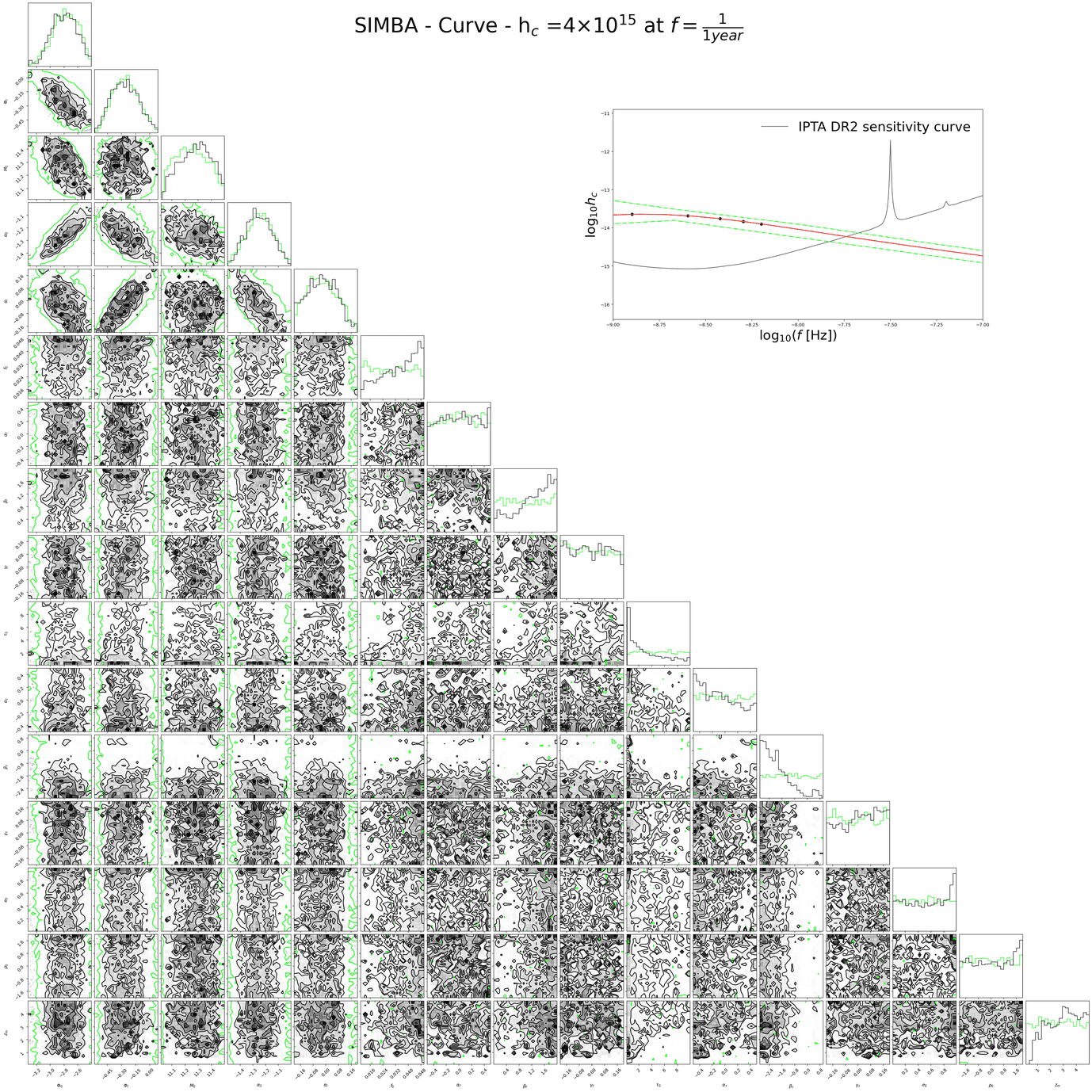
Figure 33: Corner plot of the sixteen parameters for curved line characteristic strain spectrum of $h_{c}=4\times 10^{-15}$ with black hole-bulge parameter of SIMBA is denoted by the black lines. The prior distribution is denoted by the light green lines. Top right of both figures show the characteristic spectrum of the corner plot with the allowed error range, where the 5 points denote the frequency bins of $1/25$year, $2/25$year, $3/25$year, $4/25$year and $5/25$year which is used for the Bayesian analysis to create the posterior distribution. Also just to guide the eye, the IPTA DR2 Sensitivty curve is plotted in it.

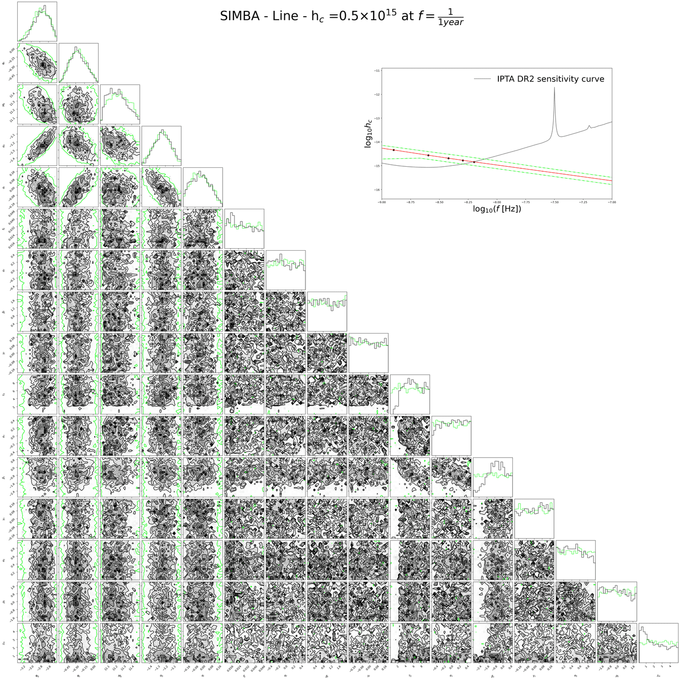
Figure 34: Corner plot of the sixteen parameters for straight line characteristic strain spectrum of $h_{c}=0.5\times 10^{-15}$ with black hole-bulge parameter of SIMBA is denoted by the black lines. The prior distribution is denoted by the light green lines. Top right of both figures show the characteristic spectrum of the corner plot with the allowed error range, where the 5 points denote the frequency bins of $1/25$year, $2/25$year, $3/25$year, $4/25$year and $5/25$year which is used for the Bayesian analysis to create the posterior distribution. Also just to guide the eye, the IPTA DR2 Sensitivty curve is plotted in it.

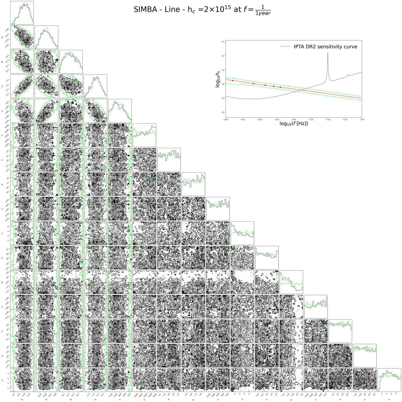
Figure 35: Corner plot of the sixteen parameters for straight line characteristic strain spectrum of $h_{c}=2\times 10^{-15}$ with black hole-bulge parameter of SIMBA is denoted by the black lines. The prior distribution is denoted by the light green lines. Top right of both figures show the characteristic spectrum of the corner plot with the allowed error range, where the 5 points denote the frequency bins of $1/25$year, $2/25$year, $3/25$year, $4/25$year and $5/25$year which is used for the Bayesian analysis to create the posterior distribution. Also just to guide the eye, the IPTA DR2 Sensitivty curve is plotted in it.

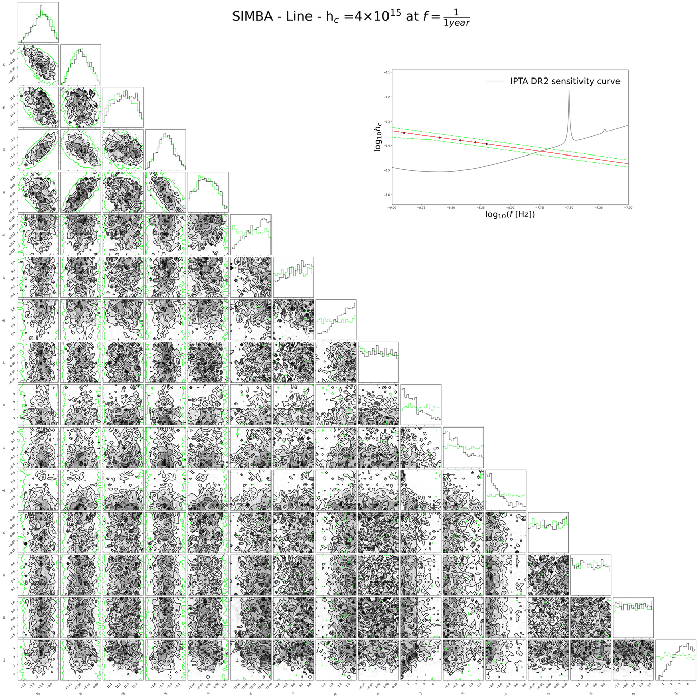
Figure 36: Corner plot of the sixteen parameters for straight line characteristic strain spectrum of $h_{c}=4\times 10^{-15}$ with black hole-bulge parameter of SIMBA is denoted by the black lines. The prior distribution is denoted by the light green lines. Top right of both figures show the characteristic spectrum of the corner plot with the allowed error range, where the 5 points denote the frequency bins of $1/25$year, $2/25$year, $3/25$year, $4/25$year and $5/25$year which is used for the Bayesian analysis to create the posterior distribution. Also just to guide the eye, the IPTA DR2 Sensitivty curve is plotted in it.

References

- Amaro-Seoane et al. (2017) Amaro-Seoane P., et al., 2017, arXiv e-prints, p. arXiv:1702.00786
- Amaro-Seoane et al. (2023) Amaro-Seoane P., et al., 2023, Living Reviews in Relativity, 26, 2
- Angulo & Hahn (2022) Angulo R. E., Hahn O., 2022, Living Reviews in Computational Astrophysics, 8, 1
- Antoniadis et al. (2022) Antoniadis J., et al., 2022, MNRAS, 510, 4873
- Arzoumanian et al. (2016) Arzoumanian Z., et al., 2016, Astrophysical Journal, 821, 13
- Arzoumanian et al. (2018) Arzoumanian Z., et al., 2018, Astrophysical Journal, 859, 47
- Arzoumanian et al. (2020) Arzoumanian Z., et al., 2020, Astrophysical Journal, 905, L34
- Bailes et al. (2020) Bailes M., et al., 2020, Publ. Astron. Soc. Australia, 37, e028
- Beifiori et al. (2012) Beifiori A., Courteau S., Corsini E. M., Zhu Y., 2012, Mon. Not. R. Astron. Soc., 419, 2497
- Bernardi et al. (2014) Bernardi M., Meert A., Vikram V., Huertas-Company M., Mei S., Shankar F., Sheth R. K., 2014, MNRAS, 443, 874
- Chen et al. (2017) Chen S., Sesana A., Del Pozzo W., 2017, MNRAS, 470, 1738
- Chen et al. (2019) Chen S., Sesana A., Conselice C. J., 2019, MNRAS, 488, 401
- Chen et al. (2021) Chen S., et al., 2021, MNRAS, 508, 4970
- Conselice et al. (2016) Conselice C. J., Wilkinson A., Duncan K., Mortlock A., 2016, Astrophysical Journal, 830, 83
- Crain et al. (2015) Crain R. A., et al., 2015, MNRAS, 450, 1937
- Davé et al. (2019) Davé R., Anglés-Alcázar D., Narayanan D., Li Q., Rafieferantsoa M. H., Appleby S., 2019, MNRAS, 486, 2827
- Desvignes et al. (2016) Desvignes G., et al., 2016, MNRAS, 458, 3341
- Detweiler (1979) Detweiler S., 1979, Astrophysical Journal, 234, 1100
- Ding et al. (2020) Ding X., et al., 2020, Astrophysical Journal, 888, 37
- Dubois et al. (2014) Dubois Y., et al., 2014, MNRAS, 444, 1453
- Dubois et al. (2016) Dubois Y., Peirani S., Pichon C., Devriendt J., Gavazzi R., Welker C., Volonteri M., 2016, MNRAS, 463, 3948
- Ellis & van Haasteren (2017) Ellis J., van Haasteren R., 2017, jellis18/PTMCMCSampler: Official Release, doi:10.5281/zenodo.1037579, https://doi.org/10.5281/zenodo.1037579
- Foster & Backer (1990) Foster R. S., Backer D. C., 1990, Astrophysical Journal, 361, 300
- Gebhardt et al. (2000) Gebhardt K., et al., 2000, Astrophysical Journal, 539, L13
- Genel et al. (2014) Genel S., et al., 2014, MNRAS, 445, 175
- Genel et al. (2018) Genel S., et al., 2018, MNRAS, 474, 3976
- Goncharov et al. (2021) Goncharov B., et al., 2021, Astrophysical Journal, 917, L19
- Graham (2012) Graham A. W., 2012, Astrophys. J., 746, 113
- Habouzit et al. (2021) Habouzit M., et al., 2021, MNRAS, 503, 1940
- Habouzit et al. (2022a) Habouzit M., et al., 2022a, MNRAS, 509, 3015
- Habouzit et al. (2022b) Habouzit M., et al., 2022b, MNRAS, 511, 3751
- Häring & Rix (2004) Häring N., Rix H.-W., 2004, Astrophysical Journal, 604, L89
- Hellings & Downs (1983) Hellings R. W., Downs G. S., 1983, The Astrophys. J.l, 265, L39
- Hobbs (2013) Hobbs G., 2013, Classical and Quantum Gravity, 30, 224007
- Hobbs et al. (2010) Hobbs G., et al., 2010, Classical and Quantum Gravity, 27, 084013
- Huerta et al. (2015) Huerta E. A., McWilliams S. T., Gair J. R., Taylor S. R., 2015, Phys. Rev. D, 92, 063010
- Jaffe & Backer (2003) Jaffe A. H., Backer D. C., 2003, Astrophysical Journal, 583, 616
- Jiang et al. (2019) Jiang P., et al., 2019, Science China Physics, Mechanics, and Astronomy, 62, 959502
- Joshi et al. (2018) Joshi B. C., et al., 2018, Journal of Astrophysics and Astronomy, 39, 51
- Kerr et al. (2020) Kerr M., et al., 2020, Publ. Astron. Soc. Australia, 37, e020
- Kormendy & Ho (2013) Kormendy J., Ho L. C., 2013, ARA&A, 51, 511
- Kramer & Champion (2013) Kramer M., Champion D. J., 2013, Classical and Quantum Gravity, 30, 224009
- Lee (2016) Lee K. J., 2016, in Qian L., Li D., eds, Astronomical Society of the Pacific Conference Series Vol. 502, Frontiers in Radio Astronomy and FAST Early Sciences Symposium 2015. p. 19
- Manchester et al. (2013) Manchester R. N., et al., 2013, Publ. Astron. Soc. Australia, 30, e017
- Marinacci et al. (2018) Marinacci F., et al., 2018, MNRAS, 480, 5113
- McConnell & Ma (2013) McConnell N. J., Ma C.-P., 2013, Astrophysical Journal, 764, 184
- Merloni et al. (2010) Merloni A., et al., 2010, Astrophysical Journal, 708, 137
- Mortlock et al. (2015) Mortlock A., et al., 2015, MNRAS, 447, 2
- Mundy et al. (2017) Mundy C. J., Conselice C. J., Duncan K. J., Almaini O., Häußler B., Hartley W. G., 2017, MNRAS, 470, 3507
- Naiman et al. (2018) Naiman J. P., et al., 2018, MNRAS, 477, 1206
- Nelson et al. (2018) Nelson D., et al., 2018, MNRAS, 475, 624
- Phinney (2001) Phinney E. S., 2001, ArXiv Astrophysics e-prints,
- Pillepich et al. (2018a) Pillepich A., et al., 2018a, MNRAS, 473, 4077
- Pillepich et al. (2018b) Pillepich A., et al., 2018b, MNRAS, 475, 648
- Pol et al. (2021) Pol N. S., et al., 2021, Astrophysical Journal, 911, L34
- Rajagopal & Romani (1995) Rajagopal M., Romani R. W., 1995, Astrophysical Journal, 446, 543
- Ravi et al. (2014) Ravi V., Wyithe J. S. B., Shannon R. M., Hobbs G., Manchester R. N., 2014, MNRAS, 442, 56
- Sampson et al. (2015) Sampson L., Cornish N. J., McWilliams S. T., 2015, Phys. Rev. D, 91, 084055
- Sani et al. (2011) Sani E., Marconi A., Hunt L. K., Risaliti G., 2011, Mon. Not. R. Astron. Soc., 413, 1479
- Sazhin (1978) Sazhin M. V., 1978, Soviet Ast., 22, 36
- Schaye et al. (2015) Schaye J., et al., 2015, MNRAS, 446, 521
- Schutte et al. (2019) Schutte Z., Reines A. E., Greene J. E., 2019, Astrophysical Journal, 887, 245
- Sesana (2013a) Sesana A., 2013a, Classical and Quantum Gravity, 30, 224014
- Sesana (2013b) Sesana A., 2013b, MNRAS, 433, L1
- Sesana et al. (2008) Sesana A., Vecchio A., Colacino C. N., 2008, MNRAS, 390, 192
- Sesana et al. (2016) Sesana A., Shankar F., Bernardi M., Sheth R. K., 2016, MNRAS, 463, L6
- Spiewak et al. (2022) Spiewak R., et al., 2022, Publ. Astron. Soc. Australia, 39, e027
- Springel et al. (2018) Springel V., et al., 2018, MNRAS, 475, 676
- Tarafdar et al. (2022) Tarafdar P., et al., 2022, Publ. Astron. Soc. Australia, 39, e053
- Venemans et al. (2016) Venemans B. P., Walter F., Zschaechner L., Decarli R., De Rosa G., Findlay J. R., McMahon R. G., Sutherland W. J., 2016, Astrophysical Journal, 816, 37
- Verbiest et al. (2016) Verbiest J. P. W., et al., 2016, MNRAS, 458, 1267
- Vogelsberger et al. (2014) Vogelsberger M., et al., 2014, MNRAS, 444, 1518
- Vogelsberger et al. (2020) Vogelsberger M., Marinacci F., Torrey P., Puchwein E., 2020, Nature Reviews Physics, 2, 42