How Two-Layer Neural Networks Learn, One (Giant) Step at a Time

Abstract

We investigate theoretically how the features of a two-layer neural network adapt to the structure of the target function through a few large batch gradient descent steps, leading to an improvement in the approximation capacity with respect to the initialization. First, we compare the influence of batch size to that of multiple (but finitely many) steps. For a single gradient step, a batch of size $n=\mathcal{O}(d)$ is both necessary and sufficient to align with the target function, although only a single direction can be learned. In contrast, $n=\mathcal{O}(d^{2})$ is essential for neurons to specialize in multiple relevant directions of the target with a single gradient step. Even in this case, we show there might exist “hard” directions requiring $n=\mathcal{O}(d^{\ell})$ samples to be learned, where $\ell$ is known as the leap index of the target. Second, we show that the picture drastically improves over multiple gradient steps: a batch size of $n=\mathcal{O}(d)$ is indeed sufficient to learn multiple target directions satisfying a staircase property, where more and more directions can be learned over time. Finally, we discuss how these directions allow for a drastic improvement in the approximation capacity and generalization error over the initialization, illustrating a separation of scale between the random features/lazy regime and the feature learning regime. Our technical analysis leverages a combination of techniques related to concentration, projection-based conditioning, and Gaussian equivalence, which we believe are of independent interest. By pinning down the conditions necessary for specialization and learning, our results highlight the intertwined role of the structure of the task to learn, the detail of the algorithm (the batch size), and the architecture (i.e., the number of hidden neurons), shedding new light on how neural networks adapt to the feature and learn complex task from data over time.

1 Introduction

A central property behind the success of neural networks is their capacity to adapt to the features in the training data. Indeed, many of the classical machine learning methods, e.g. linear or logistic regression, are specifically designed to a restricted class of functions (e.g. generalized linear functions). Others, such as kernel methods, can adapt to larger function classes (e.g. square-integrable functions), but sometimes at prohibitively many samples. Despite the limitations, these methods enjoy well-understood theoretical guarantees: they are convex (hence easy to train) and given a target function, it is well-understood how many samples are needed to achieve a target accuracy. The situation is dramatically different for neural networks: despite being universal approximators, little is known on how to optimally train them or how many hidden units and/or samples are required to learn a given class of functions. Nevertheless, they have proven to be flexible, efficient and easy to optimize in practice, properties which are often attributed to their capacity to adapt to features in the data. Curiously, most of our current theoretical understanding of neural networks stems from the investigation of their lazy regime where features are not learned during training. In this work, we take some (giant) steps forward from the lazy regime.

Our central goal is to paint a complete picture of how two-layer neural networks adapt to the features of training data $(\bm{z}^{\nu},y^{\nu})_{\nu=1}^{n}\in\mathbb{R}^{d+1}$ in the early phase of training after the first few steps of gradient descent. We recall the reader that for data is supported in a high-dimensional space, the curse of dimensionality prevents efficient learning even under standard regularity assumptions on the target function such as Lipschitzness (Devroyeetal., 2013). Hence, understanding the efficient learning performance of neural networks observed in practice requires additional assumptions on the data distribution. In this work, we focus on a popular synthetic data model consisting of: a) independently drawn standard Gaussian covariates $\bm{z}^{\nu}\sim\mathcal{N}(0,I_{d})$; b) a target function $y^{\nu}=f^{\star}(\bm{z}^{\nu})$ depending only on a finite number of relevant directions, also known as a multi-index model. In other words, there exists a finite number of orthogonal teacher vectors $\bm{w}_{1}^{\star},\dots,\bm{w}_{r}^{\star}$ such that

$$y=f^{\star}(\bm{z})\coloneqq g^{\star}(\langle\bm{w_{1}}^{\star},\bm{z}\rangle,\dots,\langle\bm{w_{r}}^{\star},\bm{z}\rangle).$$ (1)

Note that in this model the features are isotropic, with all the structure in the data being in the target. In contrast to other popular models for structured data , such as low-dimensional support of the inputs or smoothness of the target function, kernel methods do not adapt to target functions depending on low-dimensional projections bach2017breaking. This makes it an ideal playground for quantifying the adaptativity of neural networks in the feature-learning regime. Given this class of structured targets, we consider supervised learning with the simplest universal approximator neural network: a fully-connected two-layer network with first and second layer weights $W\in\mathbb{R}^{p\times d}$ and $\bm{a}\in\mathbb{R}^{p}$ and activation function $\sigma:\mathbb{R}\to\mathbb{R}$:

$$\hat{f}(\bm{z};W,\bm{a})=\frac{1}{\sqrt{p}}\sum_{i=1}^{p}a_{i}\sigma(\langle\bm{w}_{i},\bm{z}\rangle).$$ (2)

The primary focus of this work is to elucidate how a two-layer neural network adapts to a low-dimensional target structure during its training. We aim to understand the interplay among the structure of the task (specifically, the complexity of the hidden true function), the details of the algorithm (here the batch size), and the architecture (the number of hidden neurons) in the process of learning from data (zdeborova2020understanding). In particular, we will be interested in quantifying how much data is required for the relevant directions of the target to be learned, and how this feature learning translates into the approximation capacity of the network with respect to kernel methods.

2 Summary of main results

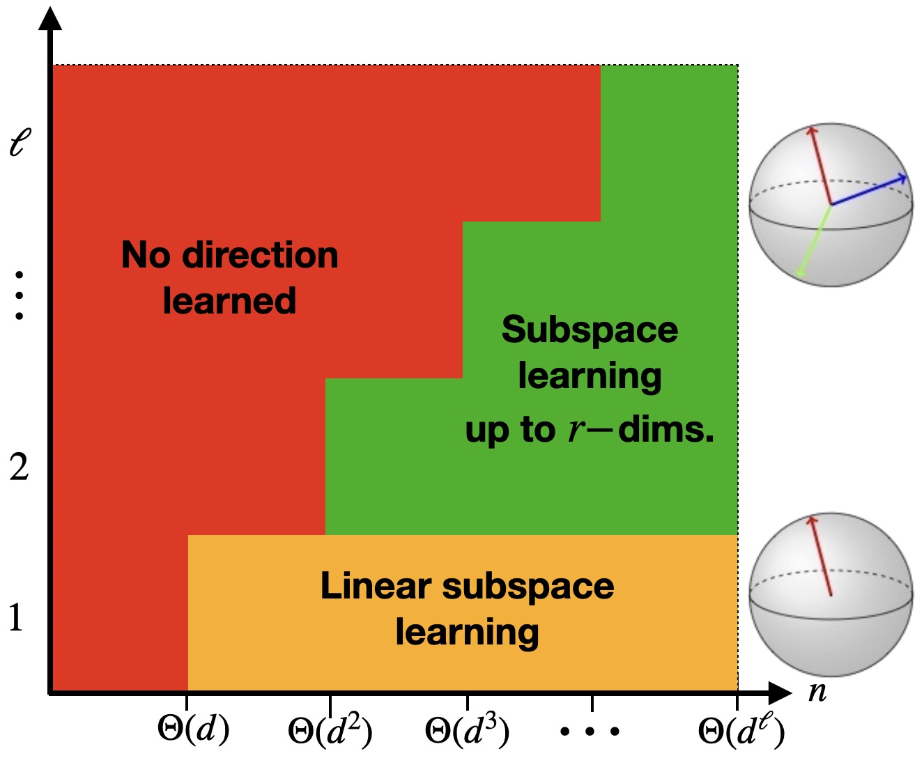
Figure 1: Learning with a single gradient step. Illustration of the relationship between batch size and target function complexity for learning multi-index functions with a single giant step in the $n=\Theta(d^{k})$ regime (Thms. LABEL:thm:one_step_lower_bound & LABEL:thm:one_step_learning).

To outperform the network at initialization (which can be regarded as a kernel method) the network must adapt to the data distribution. Mathematically, this translates to developing correlation in the first layer weights with the target directions $\bm{w}^{\star}_{1},\ldots,\bm{w}^{\star}_{r}$. Our first set of results thus precisely focus on feature learning, i.e. how the subspace

$$V^{\star}\coloneqq\operatorname{span}(\bm{w}_{1},\dots,\bm{w}_{r})$$

is learned during training.

2.1 A single Gradient step

First, we discuss the case of a single gradient step of full-batch gradient descent, which turns out to be already non-trivial (ba2022high; damian2022neural) and consider the update:

$$\bm{w}_{i}^{1}=\bm{w}_{i}^{0}-\frac{\eta}{2n}\sum_{\nu=1}^{n}\nabla_{\bm{w}_{i}}\left(y^{\nu}-\hat{f}(\bm{z}^{\nu};W^{0},\bm{a}^{0})\right)^{2}\,.$$ (3)

Theorems LABEL:thm:one_step_lower_bound and LABEL:thm:one_step_learning identify a fundamental interplay between batch size and the complexity of the underlying target function. They are summarized in Fig. 1 (and a particular numerical example is shown in Fig. LABEL:fig:example). More precisely:

• We show that developing meaningful correlation with the target function requires a large batch size $n=\mathcal{O}(d)$ and learning rate $\eta=\Theta(p)$ when $p,d,n$ are large. However, feature learning remains limited in this regime since we prove only a single direction can be learned. Thus, if the target depends on several relevant directions, only a "single neuron" approximation can be learned.

• Surpassing the single direction approximation with a single step requires a larger batch size with at least $n=\mathcal{O}(d^{2})$ samples. This allows for the network weights to specialize to multiple target directions.

• Nonetheless, we show that there might be hard directions in the target which cannot be learned with $n=\mathcal{O}(d^{2})$. Learning these directions necessitates a batch size of at least $n=\mathcal{O}(d^{\ell})$, as well as suppressing the directions learned at $n=\mathcal{O}(d^{\ell-1})$, where $\ell$ is the leap index of the target (precisely defined in Def. 3) that thoroughly speaking corresponds to the lowest non-zero degree of the Hermite polynomials in the expansion of the target in this directions.

This description paints a clear picture on how the role of the batch size, of the learning rate, and the structure of the hidden function are intertwined. The complexity of learning a low-dimensional target function is a topic that recently saw a surge of interest, and it is thus interesting to contrast these rates with recent results in the litterature.

For a single-index function with leap index $\ell$, one-pass SGD has a sample complexity of $\mathcal{O}(d^{\ell-1})$ (BenArous2021), and it has been recently shown that a smoothed version of SGD achieves a sample complexity of $\mathcal{O}(d^{\ell/2})$ (damian_2023_smoothing). This matches a lower bound from the correlation statistical query family, which encompasses all SGD-like methods. In our single step setting, the sample complexity for large batch learning is $\mathcal{O}(d^{\ell})$, which is worse than both the aforementioned methods. However, the time complexity of each algorithm paints a different picture. Both SGD algorithms are sequential, and require $\mathcal{O}(d)$ operations per step, which leads to a total time complexity of $\mathcal{O}(d^{\ell/2+1})$ at least. On the other hand, the computation of the update in Eq. LABEL:alg:gd_training is simply an average of independent terms, which is easy to parallelize. Including the time to compute the average of each term e.g. using a Gossip algorithm (boyd_2006_randomized), this sums up to a time complexity of $\mathcal{O}(d+\log(n))$. Such an algorithm is also amenable to decentralized learning schemes, where each agent only has access to a fraction of the overall data.

2.2 Learning over many GD iterations

The situation drastically improves when taking for multiple gradient steps. In this case, focusing on the linear batch size $n={\cal O}(d)$ regime, and using a fresh batch of data at each GD iteration:

$$\bm{w}_{i}^{t+1}=\bm{w}_{i}^{t}-\frac{\eta}{2n}\sum_{\nu=1}^{n}\nabla_{\bm{w}_{i}}\left(y^{\nu}-\hat{f}(\bm{z}^{\nu};W^{t},\bm{a}^{0})\right)^{2}\,,$$ (4)

Note that splitting the training of the first and second layers and using a fresh batch of data at each iteration is a common approximation in this literature (damian2022neural; ba2022high; Bietti2022). In contrast to the recent works considering the population limit, we stress that here we take the batch size $n$ to scale with the dimension $d$. In the realm of distributed and federated learning, scenarios with large batches, a single pass, and few iterations are often the norm (goyal2017accurate; li2020review) (for instance this is the case when training large language models), further underlining the relevance of this scenario. In this case, Theorem LABEL:thm:staircase shows that more complex subspaces of the target directions may be progressively learned at each iteration, as we illustrate in Fig. 2. More precisely:

• Each additional gradient step allows for learning new perpendicular directions upon the important condition that they are linearly connected to the previously learned directions (see Sec .LABEL:sec:few-giant-steps for precise definitions of this staircase property). Therefore, in contrast with a single step, taking multiple steps allows to learn a multiple-index target with only $n={\cal O}(d)$ samples.

• Nonetheless, directions that are not coupled through the staircase property and with zero first Hermite coefficient cannot be learned in any finite number of steps. In fact, as discussed previously, they require a batch size of at least $n={\cal O}(d^{2})$. In other words, while multiple steps help specialization, it cannot help learning “hard” target directions.

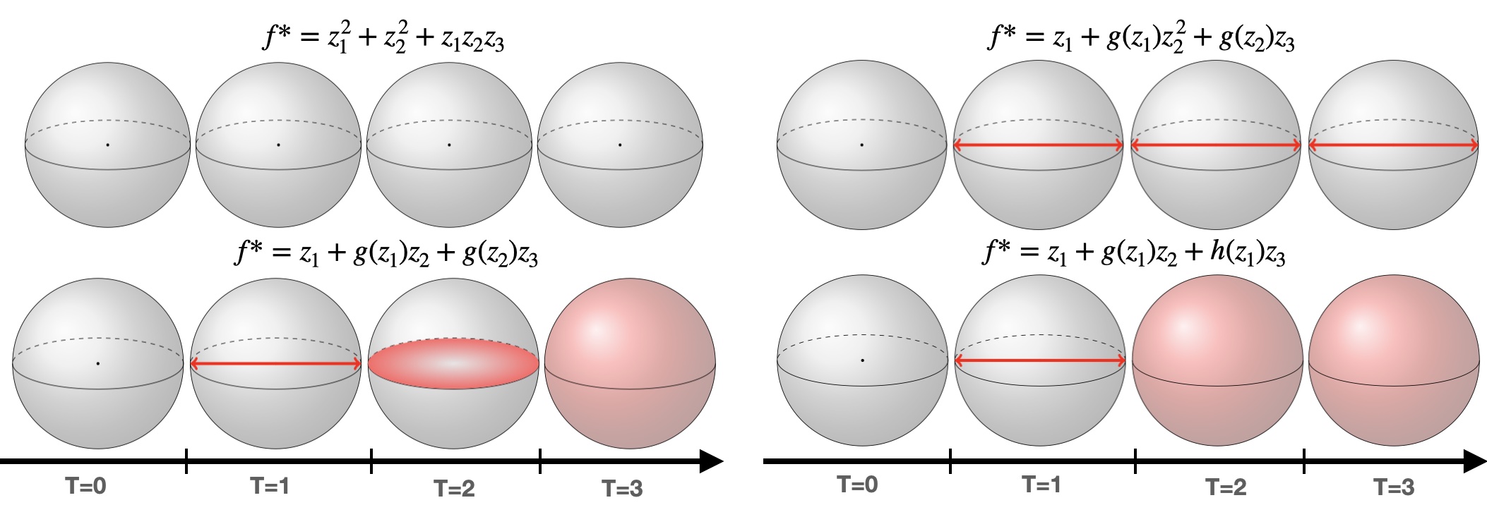
Figure 2: Learning with multiple gradient steps. An illustration of how neural networks trained using $n=\mathcal{O}(d)$ batches learn relevant directions after multiple GD training steps, allowing to learn more complex functions over time (see Thm. LABEL:thm:staircase). Here we represent the space $V^{\star}$ of the relevant direction of the target function, and the (normalized) projection of learned direction $W^{t}$ by the networks for different task $f^{\star}(\cdot)$ - the function $g(\cdot)$ and $h(\cdot)$ are assumed to have zero first two Hermite coefficients. During the early stage of training, neural networks first learn first a single direction associated to the linear part of the target, and then can learn over time other directions that are linear conditioned on the previous learned ones. Let $\{\bm{e}_{i}\}_{i\in[d]}$ be the standard basis of $\mathbb{R}^{d}$, the four examples show cases where: Top left: No directions is learned at all. Top right: The network can only learn a single direction $\bm{e}_{1}$ (single index regime). Bottom left: The network learns a new direction each time, $\bm{e}_{1}$, then $\bm{e}_{2}$ and finally $\bm{e}_{3}$. Bottom right: The network learns $\bm{e}_{1}$ at the first step and both $\bm{e}_{2}$ and $\bm{e}_{3}$ at the second steps.

These results warrant the following comments in context of the state of art. First, abbe2023sgd (following abbe2021staircase; abbe2022merged who introduced staircase functions) generalized the approach of (BenArous2021) and showed that (one-sample at a time) SGD can indeed learn staircase functions with $O(d)$ iterations and $O(d)$ samples. Using, as we do here, large batches $n_{d}=O(d)$ gives the same $O(d)$ dependence in terms of sample complexity, but allows us to learn them with $O(1)$ iterations instead. This is a nice illustration of the speed-up provided by batch-GD over SGD, as well as how large batch SGD benefits from multiple iterations over a single one (see table LABEL:table for a summary).

Secondly, we note that similar to the saddle-to-saddle dynamics under gradient flow (jacot2021saddle; abbe2023sgd; boursier2022gradient), the dynamics described through Thm.LABEL:thm:staircase involves sequential learning of directions. We note, however, that in the one-sample SGD regime (BenArous2021; abbe2023sgd) the gradient has vanishing correlation with new directions, thus requiring a polynomial number of updates to escape saddles. In contrast, the large-batch gradient updates contain a finite fraction of components along the new directions, allowing their learning through a single step. Moreover, we show that each update leads to a $\mathcal{O}(1)$ change in the components along direction in $V^{\star}$, obviating the need for coordinate-wise projections in abbe2023sgd.

The set of results described above provide a mathematical theory on how neural networks learn representations of the data over training. They corroborate, among others, the findings of kalimeris2019sgd, who observed that neural networks first fits the best linear classifier and subsequently learns functions of increasing complexity.

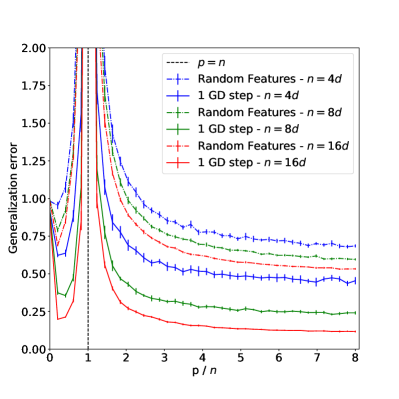
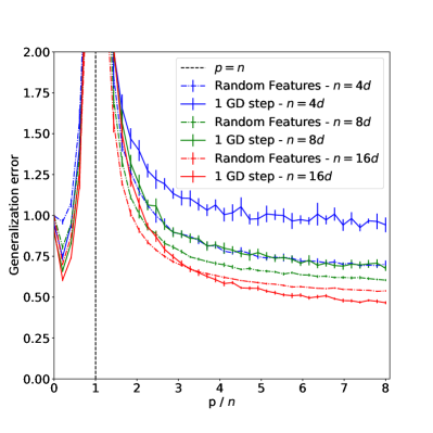
Figure 3: Feature learning and generalization: We illustrate how one step of gradient descent may (or may not) improve generalization over random features. The plot shows the generalization error as a function of the number of hidden neurons $p$ normalized by the number of samples used for the first layer training $n=\{4d,8d,16d\}$ with fixed dimension $d=2^{8}$. Left: $f^{\star}(\bm{z})=z_{1}+z_{1}z_{2}$. While random features can only fit a linear model in the proportional regime considered, one step of gradient descent over $W$ allows to fit the $z_{1}z_{2}$ part, resulting in a much lower generalization error with respect to random features, despite only the direction $z_{1}$ being learned in $W$. Right: $f^{\star}(\bm{z})=z_{1}+z_{2}z_{3}$. In this case, since the nonlinear part does not depend on $z_{1}$, one step of gradient descent on the $W$ does not allow to improve generalization over random features (see Theorem LABEL:thm:cget and Corollary LABEL:corr:lower_bound). We refer to App. LABEL:sec:appendix:numerics for details on the numerics.

2.3 From features to generalization

Our last set of results connects feature learning with the approximation capacity of the network and illustrates that feature learning improves the learning of the target function $f^{\star}$ over random initialization.

• We show that a two-layer network with a finite second layer can only learn the part of the target function in the learned subspace (see Proposition LABEL:prop:fixed_width_lower_bound). In fact, we conjecture that with $p$ large enough (but still finite), it should be possible to approximate this part of $f^{\star}$ up to arbitrary precision (Conj. LABEL:conj:approxim_conj).

• As (possibly) universal kernels, large width two-layer networks at initialization enjoy of better approximation capacity. Indeed, mei_generalization_2022 proved that at initialization $W^{t=0}$, with $n=\Theta(d^{k})$ only a degree $k$ approximation of the target function can be learned. Our results characterize how feature learning allows us to improve over this sample complexity. In particular, we show that in the directions learned by the first layer, the target function $f^{\star}$ can be learned with less samples, while the component of $f^{\star}$ orthogonal to the learned features still requires $n=\mathcal{O}(d^{k})$. While a complete mathematical control of the generalization error rates remains a difficult problem (see Conjecture LABEL:conj:kernel+feature), our results provide a clear separation on scales between two-layer networks and NTK-like methods, improving over the state-of-the art in the literature.

• In particular, in Corollary LABEL:corr:lower_bound we prove that with a single gradient step and $n,p=\mathcal{O}(d)$, one can only learn features in this one-dimensional subspace, doing no better than kernels in the orthogonal direction. This is illustrated in Fig.3 where we give an example where one step of gradient drastically improves generalization, and one where it does not. To prove these results, we provide a stronger conditional version of the Gaussian equivalence theorem (mei_generalization_2022; goldt_gaussian_2021; hu2022universality), which is the backbone of Theorem LABEL:thm:cget, and we believe is of independent interest.

The code to reproduce our figures is available on GitHub, and we refer to App. LABEL:sec:appendix:numerics for details on the numerical implementations. Proofs are detailed in App. LABEL:sec:appendix:gd_proofs and App. LABEL:sec:appendix:cget_proofs.

Other related works —

The analysis of high-dimensional asymptotics of kernel regression has provided valuable insights into the advantages and limitations of kernel methods (Dietrich1999; Opper2001; Ghorbani2019; Ghorbani2020; Donhauser2021; Mei2023; Spigler2020; bordelon20a; Canatar2021; simon2022eigenlearning; Cui2021; Cui2022; xiao2022precise). In particular, a similar stairway picture as in Fig. 2 emerged from these works xiao2022precise. The key difference, however, is that at each regime $n={\cal O}(d^{k})$, kernels can only learn the $k$-th Hermite polynomial of the target. This should be contrasted with our feature learning regime where, once a direction is learned, all its Hermite coefficients are learned. Feature learning corrections to kernel methods have been investigated in pmlr-v75-dudeja18a; Naveh2021; Seroussi2023; atanasov2022neural; Bietti2022; bordelon2023dynamics; petrini2022learning. On a complementary line of work, exact asymptotic results for the the random features models have been derived in the literature (mei_generalization_2022; gerace_generalisation_2020; Dhifallah2020; loureiro_learning_2021; loureiro22a; schroder2023deterministic; bosch2023precise). A large part of these results are enabled by the Gaussian equivalence property (goldt_gaussian_2021; hu2022universality; Montanari2022; dandi2023universality).

Closer to us are (ba2022high; damian2022neural). ba2022high showed that a sufficiently large single gradient step allows to beat kernel methods. ba2022high showed that a single gradient step yields an approximately rank-one change on the weights which is enough to beat kernel methods, but did not characterize the impact on the generalization error. In our work, we prove that with a single gradient step and $n,p=\mathcal{O}(d)$, one can only learn features in this one-dimensional subspace, doing no better than kernels in the orthogonal direction. Additionally, their results are limited to single-index target and to a single gradient step. In contrast, damian2022neural showed that with $n=\omega(d^{2})$ samples, two-layer neural networks can specialize to more than one direction of a multi-index target function with zero first Hermite coefficient ($\ell$=2), and were again limited to a single step. Our work extends their sufficient conditions on the sample complexity to general $\ell\geq 1$. We also show they are also necessary, i.e. $\forall\epsilon>0$, with less data $n=\Theta(d^{\ell-\epsilon})$ one cannot do better than random features. Thus, our results prove a clear separation between the class of functions learned within the $\Theta(d)$ batch-size setting of ba2022high and the $\Theta(d^{2})$ batch-size setting of damian_2023_smoothing and establish a general hierarchy of functions requiring increasing batch-size to be learned with a gradient step. Additionally, we characterize which class of multi-index targets can be instead learned with $n=\mathcal{O}(d)$ with multiple steps.

In a related but different vein, abbe2022merged, building upon the earlier work of abbe2021staircase show how a “staircase" property of target functions characterizes the sample complexity for infinite width two-layer networks trained by SGD, a.k.a. the mean-field regime mei2018mean; chizat2018global; rotskoff2018trainability; sirignano2020mean). Their focus, however, was on the peculiar case of sparse boolean functions depending solely on linear coefficients, without considering direction-specific specialization. More recently, abbe2023sgd provided partial results for the case of isotropic Gaussian data, always in the regime of one-pass SGD, involving basis-dependent projections. Here we consider the more generic case of multi-index target functions with Gaussian data with large-batch SGD, without the use of a knowledge of the basis, and show that a “directional staircase" behavior arises when iterating a few giant gradient steps, while a related, but definitely different, picture arises with single steps depending on the batch size. We also provide a sharp characterization of when this phenomenon appears for multi-index targets and networks trained under large batch SGD, and provide a bound on the resulting generalization error.

Similar to the “summary statistics" approach in saad.solla_1995_line; BenArous2021; ben2022high, our analysis is based upon the concentration of the overlaps of the neurons with the target subspace and their norms, instead of the concentration of the full gradient vector considered in recent works such as abbe2022merged; damian2022neural, removing any requirements on the constants in the sample complexity for alignment along the target subspace.

3 Statement of main theoretical results

3.1 Preliminaries

Before stating our main results, we recall a few definition and useful facts.

Hermite expansion —

Given the Gaussian measure $\gamma_{m}$ on $\mathbb{R}^{m}$, we can build a scalar product on $\ell^{2}(\mathbb{R}^{m},\gamma_{m})$ as

$$\langle f,g\rangle_{\gamma}=\int_{\mathbb{R}^{m}}fg\ \mathrm{d}\gamma_{m}=\mathbb{E}_{\bm{z}\sim\mathcal{N}(\bm{0},I_{m})}[f(\bm{z})g(\bm{z})].$$ (5)

It turns out that there is a specific orthonormal basis of interest for this scalar product, that we present in tensor form:

Definition 1 (Hermite decomposition).

Let $f:\mathbb{R}^{m}\to\mathbb{R}$ be a function that is square integrable w.r.t the Gaussian measure. There exists a family of tensors $(C_{j}(f))_{k\in\mathbb{N}}$ such that $C_{j}(f)$ is of order $j$ and for all $\bm{x}\in\mathbb{R}^{m}$,

$$f(\bm{x})=\sum_{j\in\mathbb{N}}\langle C_{j}(f),\mathcal{H}_{j}(\bm{x})\rangle$$ (6)

where $\mathcal{H}_{j}(\bm{x})$ is the $j$-th order Hermite tensor (grad_1949_note).

Higher-order singular value decomposition —

The higher-order singular value decomposition (HOSVD) of a tensor is defined as follows:

Definition 2 (Higher-order SVD).

Let $C\in\mathbb{R}^{m^{k}}$ be a symmetric tensor of order $k$. A higher-order SVD of $C$ is an orthonormal set $(\bm{u}_{1},\dots,\bm{u}_{r})$ of $r\leq k$ vectors, as well as a tensor $S\in\mathbb{R}^{r^{k}}$ such that

$$C=\sum_{j_{1},\dots,j_{k}=1}^{r}S_{j_{1},\dots,j_{k}}\bm{u}_{j_{1}}\otimes\dots\otimes\bm{u}_{j_{k}}$$ (7)

The singular values tensor $S$, as well as the rank $r$, are unique, but just as the regular SVD, the vectors $(\bm{u}_{1},\dots,\bm{u}_{r})$ are only unique up to rotations.

3.2 Setting and assumptions

Before stating our main results, we introduce the setting and main assumptions required. The first concerns the class of target functions we consider.

Assumption 1 (Data model).

The training inputs $\bm{z}^{\nu}\in\mathbb{R}^{d}$ are independently drawn from the Gaussian distribution $\mathcal{N}(0,I_{d})$. Further, we assume that the target function $y^{\nu}=f^{\star}(\bm{z})$ depends only on a few relevant directions. In other words, there exists a fixed number of orthonormal vectors $(\bm{w}_{1},\dots,\bm{w}_{r})$ and a fixed function $g^{\star}:\mathbb{R}^{r}\to\mathbb{R}$ such that

$$y=f^{\star}(\bm{z})\coloneqq g^{\star}(\langle\bm{w_{1}}^{\star},\bm{z}\rangle,\dots,\langle\bm{w_{r}}^{\star},\bm{z}\rangle).$$ (8)

As we will show later, learning with GD can be seen as a hierarchical process, where depending on the batch size different directions of the target are progressively learned. Next, we define the leap index, a fundamental quantity which precisely parametrizes what are the first directions to be learned.

Definition 3 (Leap index).

Since the input data is Gaussian $\bm{z}\sim\mathcal{N}(0,I_{d})$, the target function admits a decomposition in terms of the Hermite decomposition (see Definition 1). We define the leap index of the target function $f^{\star}$ as the first integer $\ell>0$ such that $C_{\ell}^{\star}\neq 0$:

$$\ell=\min\{j\in\mathbb{N}:\langle f^{\star},\mathcal{H}_{j}\rangle_{\gamma}\neq 0\}$$ (9)

Given a batch of training data $(\bm{z}^{\nu},y^{\nu})_{\nu=1}^{n}\in\mathbb{R}^{d+1}$ drawn from the model (1) defined above, we now define how the network weights $(W,a)$ are initialized and updated.

Assumption 2 (Training procedure).

Consider the following random initialization for the weights:

$$\sqrt{p}\cdot a{}_i{}^0\stackrel{i.i.d}{\sim }\mathrm{Unif}\left(\right[-1,1\left]\right)\text{References12013Devroyeetal.D}$$ (10)