MLE for the parameters of bivariate interval-valued model

Abstract

With contemporary data sets becoming too large to analyze the data directly, various forms of aggregated data are becoming common. The original individual data are points, but after aggregation the observations are interval-valued (e.g.). While some researchers simply analyze the set of averages of the observations by aggregated class, it is easily established that approach ignores much of the information in the original data set. The initial theoretical work for interval-valued data was that of Le-Rademacher and Billard (2011), but those results were limited to estimation of the mean and variance of a single variable only. This article seeks to redress the limitation of their work by deriving the maximum likelihood estimator for the all important covariance statistic, a basic requirement for numerous methodologies, such as regression, principal components, and canonical analyses. Asymptotic properties of the proposed estimators are established. The Le-Rademacher and Billard results emerge as special cases of our wider derivations.

1 Introduction

Le-Rademacher and Billard (2011) derived the maximum likelihood estimator (MLE) of the mean and variance when the data consisted of interval-valued observations. In this work, our primary focus is to extend that work to derive the MLE for the covariance function between the random variables $(X,~{}Y)$ when both $X$ and $Y$ are interval-valued. The covariance function is of particular importance given its major role in covariance matrices used in principal component analyses, canonical analyses, as well as the entries/components in the “${\bf X}^{\prime}{\bf X}$” and “${\bf Y}^{\prime}{\bf X}$” terms in multiple regression analyses, among other methodologies; yet so far no maximum likelihood estimator currently exists for this key entity.

Maximum likelihood estimation is arguably the most important method of parameter estimation in statistics. Traditionally, the data analyzed are so-called classical data in which each data value is a single point. However, with the advent of modern computers and data collecting devices, contemporary data sets are becoming too large and too complicated to be analyzed directly. One approach has been to aggregate the observations into classes or categories of observations, with the nature of the aggregation varying depending on the underlying scientific questions. One consequence of this phenomena is that the data to be analyzed are no longer single points. Instead, they are so-called symbolic data first identified by Diday (1988). Thus, rather than the points of classical data, symbolic data are hypercubes (or Cartesian products of distributions). That is, for each variable, realizations can be intervals, lists, histograms, or so on. For example, an interval realization can be $[10,30]$ in contrast to a classical point observation $20$. One distinguishing feature of such data is that realizations (e.g., intervals) have internal variations that are not present in the point values of classical data. Taking classical surrogates (e.g., interval midpoints) ignores these internal variations and in doing so throws away valuable information inherent to the observations thus producing results that are not necessarily correct. Many methodologies transform the single interval-valued $X=[a,b]$ say, into two variables $X^{c}=(a+b)/2$ and $X^{r}=(b-a)/2$, center and range variables (or equivalently into $X_{a}=a$ and $X_{b}=b$, the two end points). While this is an improvement on using $X^{c}$ only, the resulting analyses can give inaccurate answers; as illustrated in Appendix A. Recently, Oliveira et al. (2017, 2022) proposed a model, based on functions of the centers and ranges, linking the micro-data (un-aggregated observations) that made up the macro-data (interval) and thence looked at eight possible formulations in an effort to tie together proposed covariance functions from the literature.

Many methodologies for symbolic datasets have been developed since Diday (1988) introduced the concept. By and large, these are intuitive extensions of their classical counterparts, although accommodating the internal variations of symbolic data make these extensions far from trivial. However, since classical data are a special case of symbolic data (e.g., the classical value $x$ is equivalent to the interval value $[x,\,x]$), obtaining the established classical results as a special case of the symbolic techniques is one form of verification as to their correctness. Deriving theoretical foundations for these methodologies has been more difficult to achieve. Some results do however exist. Thus, Diday (1995), Diday, Emilion and Hillali (1996), Emilion (1997), and Diday and Emilion (1996, 1998) obtained a mathematical framework for some classes of symbolic data. Then, Diday and Emilion (1998, 2003) and Brito and Polaillon (2005) extended those results to Galois lattices used in, e.g., pyramid clustering. Later, Le-Rademacher and Billard (2011) obtained maximum likelihood estimators for the mean and variance of a univariate distribution when the observations were interval-valued. More recently, Zhang et al. (2020) and Beranger et al. (2022) provided a framework for likelihood functions for interval data, which results were then used to consider the variance-covariance function in regression; see Whitaker et al. (2020, 2021), and Rahman et al. (2020). Samadi and Billard (2021) looked at auto-covariances for interval-valued time series observations. Beyond these results, almost no mathematical theoretical underpinnings for symbolic methodology have yet been fully established.

First in Section 2, we describe symbolic data especially interval-valued data, along with some of the basic descriptive statistics for these data. Then in Section 3, we establish a likelihood function, and derive in Section 4.1 some maximum likelihood estimators for the parameters of the proposed model. Hence, by utilizing the ideas behind first and second order conditional moments, we show that the empirically based descriptive statistics (of Section 2) are maximum likelihood estimators (or, approximately so); see Section 4.2. Asymptotic properties of proposed estimators are studied in Section 5. In Section 6, we consider some extensions where the internal spread across the intervals is non-uniform. Then, in Section 7, a short simulation study is conducted; and the results are illustrated through an analysis of real data.

2 Symbolic Data

A major source of symbolic data arises when managing large contemporary data sets. For example, a medical insurer may have a database of client visits to a health-care entity (doctor, hospital, etc.) with entries recording values for a variety of variables, such as basic medical information (e.g., weight, cholesterol, blood pressure, …), or demographic information (gender, age, …), disease diagnosis (e.g., cancer with a list of cancers presenting, heart disease with a list of heart conditions, and so on), clinical diagnostics, geographical variables, and more. The insurer (or investigator, or …) is not so much interested in a particular visit to the doctor as s/he might be interested in the health characteristics of categories of clients. However, symbolic data can also occur naturally. For example, the pileus cap width of mushroom species is usually recorded as intervals; interval data can also be used to protect confidentialities; daily temperatures are recorded as minimum-maximum temperatures, e.g., $[38,56]$. Bock and Diday (2000) and Billard and Diday (2003, 2006) have extensive detailed descriptions and examples of symbolic-valued data, including intervals.

It is important to remind ourselves that although observations may be aggregated into intervals (say), the underlying distributions are still the traditional (classical) distributions with their relevant parameters. That is, after aggregation, the original classical values still retain their same distributions. What has changed is the format of the realization of the observation to become, e.g., an interval-valued observation. Indeed, Bertrand and Goupil (2000) obtained the sample mean and the sample variance for a sample of interval-valued observations as point estimators of the parameters $\mu$ and $\sigma^{2}$. For the symbolic-valued interval, additional assumptions are made as to how those aggregated observations are spread within a given interval however. The Bertrand and Goupil results assume the observations are uniformly spread across the intervals. As an aside, we note this uniformly assumption is comparable to that used in finding the histogram of grouped data as taught in elementary statistics classes. We note that this is not the same as interval-arithmetic concepts (which would give parameters themselves as interval-values, e.g., $\mu=(\mu_{1},\mu_{2})$; see, e.g., Moore, 1966). The interval-arithmetic domain is quite different from the symbolic-valued data domain, and is not considered herein.

Interval-valued data are, as the name suggests, realizations of a random variable $Y$, that are intervals $[a_{i},~{}b_{i}]$, $a_{i}\leq b_{i}$, $i=1,\dots,n$, for a random sample of size $n$. [Intervals can be open or closed at either end.] Now, the observable interval is essentially an (aggregated) group of observations, while the unobservable individual data are scalar. Therefore, the underlying parameters and descriptive statistics, such as the sample mean and variance, are also scalar entities. Bertrand and Goupil (2000) first obtained expressions for the empirical (sample) mean $\bar{Y}$ and variance $S^{2}_{Y}$ as

$$\bar{Y} =\frac{1}{2n}\sum_{i=1}^{n}(a_{i}+b_{i}),$$ (1)

$$S^{2}_{Y} =\frac{1}{3n}\sum_{i=1}^{n}(a_{i}^{2}+a_{i}b_{i}+b_{i}^{2})-\bar{Y}^{2}/n\equiv S_{YY}\mbox{, say}.$$ (2)

Let us also have a second random variable $X$ with interval-valued realizations $[c_{i},\,d_{i}]$, $i=1,\dots,n$, for a random sample of size $n$. Billard (2008) obtained the empirical sample covariance function as

$$\begin{split}S_{XY}&=\frac{1}{6n}\sum_{i=1}^{n}[2(a_{i}-\bar{Y})(c_{i}-\bar{X})+(a_{i}-\bar{Y})(d_{i}-\bar{X})\\ &~{}~{}~{}~{}~{}~{}~{}~{}~{}~{}~{}~{}~{}~{}~{}~{}~{}~{}~{}~{}~{}~{}~{}~{}+(b_{i}-\bar{Y})(c_{i}-\bar{X})+2(b_{i}-\bar{Y})(d_{i}-\bar{X})]\end{split}$$ (3)

where $\bar{Y}$ is as given in Eq.(1) and $\bar{X}=\frac{1}{2n}\sum_{i=1}^{n}(c_{i}+d_{i})$. When $Y=X$, then Eq.(3) becomes $S_{XX}\equiv S_{X}^{2}$. For the special case of classical data where $a_{i}=[a_{i},\,a_{i}]$ and $c_{i}=[c_{i},\,c_{i}]$, the formulas in Eqs.(1)-(3) all reduce to their well-known classical counterparts.

An implicit assumption in the derivation of these empirical results is that observations within intervals are uniformly spread across the interval. Billard (2008) showed how the results can be extended to the non-uniform case illustrating with a triangular distribution. Since however most methodology for interval data are based on this uniformly spread assumption, our maximum likelihood approach that follows will retain this assumption. Cariou and Billard (2015) provides a test for this basic but important assumption.

3 Symbolic Likelihood Function

As in the preceding sections, suppose we have two random variables ($X,Y$) with interval-valued realizations ($X_{i},Y_{i}$) where $X_{i}=x_{i}=[c_{i},d_{i}]$ and $Y_{i}=y_{i}=[a_{i},b_{i}]$ for $i=1,\dots,n$. Let ($X_{i},\,Y_{i}$) have joint (bivariate) probability density function (pdf) $h_{X,Y}(x,y;\mbox{\boldmath$\delta$})$ with parameter $\delta$. Classes of inferential results when realizations of $(X,\,Y)$ are classical point values in $\mathbb{R}^{2}$ are well established (see, e.g., Casella and Berger, 2002; Lehmann, 1983, 1986). Our focus however is for interval-valued realizations. We adapt the approach of Le-Rademacher and Billard (2011) for univariate interval-valued random variables.

Since each variable has aggregated observed values over an interval, we need to consider the internal distribution of those values within the interval. Therefore, let the joint and marginal internal distributions be defined by, respectively, for $i=1,\dots,n$,

$$\mbox{Within }(X_{i},Y_{i})\sim f_{i}^{xy}(x_{i},y_{i};{\bf\Theta}_{i}^{xy}),\mbox{Within }(X_{i})\sim f_{i}^{x}(x_{i};{\bf\Theta}_{i}^{x}),\mbox{Within }(Y_{i})\sim f_{i}^{y}(y_{i};{\bf\Theta}_{i}^{y}).$$ (4)

These distributions $f_{i}^{xy}$, $f_{i}^{x}$ and $f_{i}^{y}$ along with their parameters ${\bf\Theta}_{i}^{xy}$, ${\bf\Theta}_{i}^{x}$ and ${\bf\Theta}_{i}^{y}$ are internal (or “within” observation) entities, distinct from the overall distributions $h_{X,Y}(x,y;\mbox{\boldmath$\delta$})$. Consistent with current symbolic data analyses methodology for interval observations, suppose the internal distributions within the ($X,Y$) intervals, i.e., the $f_{i}^{x}(x_{i};{\bf\Theta}_{i}^{x})$ and $f_{i}^{y}(y_{i};{\bf\Theta}_{i}^{y})$ of Eq.(4), are uniformly distributed, for each $i=1,\dots,n$. Hence, for the intervals $Y_{i}$, realizations of $\Theta_{i1}^{y}$ are $\theta_{i1}^{y}=(a_{i}+b_{i})/2$; and likewise for the intervals $X_{i}$ realizations of $\Theta_{i1}^{x}$ are $\theta_{i1}^{x}=(c_{i}+d_{i})/2$. The variation variables $\Theta_{i2}^{x},\Theta_{i2}^{y},\Theta_{i2}^{xy}$, respectively, have realizations $\theta_{i2}^{y}=(b_{i}-a_{i})^{2}/12$, $\theta_{i2}^{x}=(d_{i}-c_{i})^{2}/12$ and $\theta_{i2}^{xy}=(b_{i}-a_{i})(d_{i}-c_{i})/12$.

Also, since $(X_{i},Y_{i}),~{}i=1,\dots,n,$ are random variables, the parameters $({\bf\Theta}_{i}^{x},{\bf\Theta}_{i}^{y})$ are not fixed, taking different values as $(X_{i},Y_{i})$ change with $i=1,\dots,n$. That is, $({\bf\Theta}_{i}^{x},{\bf\Theta}_{i}^{y})$ are themselves random variables. Therefore, let the underlying distribution of $({\bf\Theta}_{i}^{x},{\bf\Theta}_{i}^{y})$ be

$$({\bf\Theta}_{i}^{x},{\bf\Theta}_{i}^{y})\sim g_{xy}({\bf\Theta}_{i}^{x},{\bf\Theta}_{i}^{y};\mbox{\boldmath$\tau$}_{xy}),~{}i=1,\dots,n.$$ (5)

Then for these parametric families $g_{xy}({\bf\Theta}_{i}^{x},{\bf\Theta}_{i}^{y};\mbox{\boldmath$\tau$}_{xy})$ with parameter $\mbox{\boldmath$\tau$}_{xy}$, there exist one-to-one correspondences between the $(X_{i},Y_{i})$ and $({\bf\Theta}_{i}^{x},{\bf\Theta}_{i}^{y})$. To illustrate this one-to-one correspondence, for the uniform case, assume that $X$ (similarly, for $Y$) has realization

• $x=[c,d]=[1,3]$; then $\theta_{i}^{x}=2$, $\theta_{2}^{x}=1/3$.

• If $\theta_{i}^{x}=u$, $\theta_{2}^{x}=\omega>0$, then $c+d=2u$ and $(d-c)^{2}=12\omega$.

It can be shown that for $c<d$, we have $c=u-\sqrt{3\omega}$, $d=u+\sqrt{3\omega}$. When $u=2$, $\omega=1/3$, we obtain $x=[c,d]=[1,3]$, as required.

Therefore, because of this one-to-one correspondence, we have

$$h_{X,Y}(x_{i},y_{i};\mbox{\boldmath$\delta$})=g_{xy}({\bf\Theta}_{i}^{x},{\bf\Theta}_{i}^{y};\mbox{\boldmath$\tau$}_{xy}).$$ (6)

We note that the parameters $\delta$ relate to the overall distribution $h_{X,Y}(x,y;\mbox{\boldmath$\delta$})$, and the parameters $\mbox{\boldmath$\tau$}_{xy}$ relate to the internal distributions of the (${\bf\Theta}_{i}^{x},{\bf\Theta}_{i}^{y}$) variables. Therefore, given the one-to-one correspondence between $(X_{i},Y_{i})$ and $({\bf\Theta}_{i}^{x},{\bf\Theta}_{i}^{y})$, then there is a one-to-one correspondence between $\bm{\delta}$ and $\bm{\tau}_{xy}$. The components of this $\bm{\tau}_{xy}$ will depend on the internal variation distributions $f_{i}^{x}(x_{i};{\bf\Theta}_{i}^{x})$ and $f_{i}^{y}(y_{i};{\bf\Theta}_{i}^{y})$ as shown in the next Section 4.1.

We can write the likelihood function of the parameter $\delta$ given the data $(X_{i},Y_{i})=(x_{i},y_{i}),~{}i=1,\dots,n,$ as

$$L(\mbox{\boldmath$\delta$};(x_{1},y_{1}),\dots,(x_{n},y_{n}))=\prod_{i=1}^{n}h_{X,Y}(x_{i},y_{i};\mbox{\boldmath$\delta$});$$ (7)

and substituting from Eq.(6), we have

$$L(\mbox{\boldmath$\delta$};(x_{1},y_{1}),\dots,(x_{n},y_{n}))=\prod_{i=1}^{n}g_{xy}(\mbox{\boldmath$\theta$}_{i}^{x},\mbox{\boldmath$\theta$}_{i}^{y};\mbox{\boldmath$\tau$}_{xy})=L(\mbox{\boldmath$\tau$}_{xy};\mbox{\boldmath$\theta$}_{1}^{x},\dots,\mbox{\boldmath$\theta$}_{n}^{x},\mbox{\boldmath$\theta$}_{1}^{y},\dots,\mbox{\boldmath$\theta$}_{n}^{y})$$ (8)

where $\mbox{\boldmath$\theta$}_{i}^{x},\mbox{\boldmath$\theta$}_{i}^{y}$ are realizations of $\mbox{\boldmath$\Theta$}_{i}^{x},\mbox{\boldmath$\Theta$}_{i}^{y}$, $i=1,\dots,n$.

Note that when there is independence, the product of the marginal distributions can replace the joint distribution $g_{xy}(\mbox{\boldmath$\Theta$}_{i}^{x},\mbox{\boldmath$\Theta$}_{i}^{y};\mbox{\boldmath$\tau$}_{xy})$ in Eq.(6), i.e., we have for $\mbox{\boldmath$\Theta$}_{i}^{x}$ and $\mbox{\boldmath$\Theta$}_{i}^{y}$, respectively,

$${}\mbox{\boldmath$\Theta$}_{i}^{x}\sim g^{x}(\mbox{\boldmath$\Theta$}_{i}^{x};\mbox{\boldmath$\tau$}^{x}),~{}~{}~{}\mbox{\boldmath$\Theta$}_{i}^{y}\sim g^{y}(\mbox{\boldmath$\Theta$}_{i}^{y};{\bf\tau}^{y}),~{}~{}i=1,\dots,n.$$

Since the data $(\mbox{\boldmath$\theta$}_{1}^{x},\dots,\mbox{\boldmath$\theta$}_{n}^{x},\mbox{\boldmath$\theta$}_{1}^{y},\dots,\mbox{\boldmath$\theta$}_{n}^{y})$ in Eq.(8) are now classically valued observations, we can apply maximum likelihood methods for classical data to estimate the parameters of interest. This is done in Section 4.

4 Maximum Likelihood Estimators

In Section 4.1, we obtain the maximum likelihood estimators for the within observation parameters. Then in Section 4.2, these are used to obtain the overall (within plus between) variation estimators.

4.1 Estimators for Within Observation Parameters

Let us take the internal parameters ${\bf\Theta}_{i}^{x}$ associated with $X_{i}$ and ${\bf\Theta}_{i}^{y}$ associated with $Y_{i},~{}i=1,\dots,n,$ introduced in Section 3 as ${\bf\Theta}_{i1}=(\Theta_{i1}^{x},\Theta_{i1}^{y})$ and ${\bf\Theta}_{i2}=(\Theta_{i2}^{x},\Theta_{i2}^{y},\Theta_{i2}^{xy})$. That is, we let the $\Theta_{i1}^{x}$ and $\Theta_{i1}^{y}$ correspond to the internal mean of $X_{i}$ and $Y_{i}$, respectively, for each $i=1,\dots,n$; and the $\Theta_{i2}^{x}$ and $\Theta_{i2}^{y}$ correspond to the internal variation of $X_{i}$ and $Y_{i}$, respectively, and $\Theta_{i2}^{xy}$ corresponds to the covariance of $(X_{i},Y_{i})$ for each $i=1,\dots,n$. At this stage, it is necessary to specify distributions governing these internal parameters. It is not unreasonable to consider the corresponding conjugate distribution as the respective distribution. Therefore, if the underlying individual observations (i.e., non-aggregated data) are assumed to be normally distributed (or asymptotically so), then the conjugate distribution for the internal mean parameters is normally distributed. Likewise, given its conjugate role for covariance functions and its associated property of being non-negative definite and symmetric, the Wishart (1928) distribution is used for the internal variance-covariance parameters. However, other underlying distributions could be considered.

Formally, for each $i=1,\dots,n,$ suppose that the joint distribution of the internal means ${\bf\Theta}_{i1}=(\Theta_{i1}^{x},\Theta_{i1}^{y})$ is a bivariate normal distribution $N_{2}(\mu_{x},\mu_{y},\sigma_{x}^{2},\sigma_{y}^{2},\rho)$; and suppose ${\bf\Theta}_{i2}=(\Theta_{i2}^{x},\Theta_{i2}^{y},\Theta_{i2}^{xy})$ follows a bivariate Wishart distribution (originally derived by Fisher, 1915) defined by

$$\begin{split}f(\theta_{2}^{x},\theta_{2}^{y},\theta_{2}^{xy};\gamma_{1},\gamma_{2},\gamma_{3})&=\frac{\left(\gamma_{1}\gamma_{2}-\gamma_{3}^{2}\right)^{-\frac{\nu}{2}}}{2\sqrt[\nu]{\pi}\Gamma(\frac{\nu}{2})\Gamma(\frac{\nu-1}{2})}\left(\theta_{2}^{x}\theta_{2}^{y}-(\theta_{2}^{xy})^{2}\right)^{\frac{\nu-3}{2}}\\ &~{}~{}~{}~{}~{}~{}~{}~{}~{}~{}\times\exp\left\{-\frac{\gamma_{1}\gamma_{2}}{2(\gamma_{1}\gamma_{2}-\gamma_{3}^{2})}\left(\frac{\theta_{2}^{x}}{\gamma_{1}}+\frac{\theta_{2}^{y}}{\gamma_{2}}-\frac{2\gamma_{3}\theta_{2}^{xy}}{\gamma_{1}\gamma_{2}}\right)\right\}\end{split}$$ (9)

where $\nu>2$ is the degree of freedom, $\theta_{2}^{x}>0$, $\theta_{2}^{y}>0$, and $-\sqrt{\theta_{2}^{x}\theta_{2}^{y}}<\theta_{2}^{xy}<\sqrt{\theta_{2}^{x}\theta_{2}^{y}}$ (see Anderson, 2003). Then, the joint probability density function $g_{xy}({\bf\Theta}_{i}^{x},{\bf\Theta}_{i}^{y};\mbox{\boldmath$\tau$}_{xy})$ of Eq.(5) can be written as, with $\mbox{\boldmath$\tau$}_{xy}=(\mu_{x},\mu_{y},\sigma_{x}^{2},\sigma_{y}^{2},\rho,\gamma_{1},\gamma_{2},\gamma_{3})$,

$$g_{xy}({\bf\Theta}_{i1},{\bf\Theta}_{i2};\mbox{\boldmath$\tau$}_{xy})=g_{1}(\Theta_{i1}^{x},\Theta_{i1}^{y};\mu_{x},\mu_{y},\sigma_{x}^{2},\sigma_{y}^{2},\rho)\times g_{2}(\Theta_{i2}^{x},\Theta_{i2}^{y},\Theta_{i2}^{xy};\gamma_{1},\gamma_{2},\gamma_{3}).$$ (10)

Let us write the likelihood function based on the intervals, $L_{I}$, from Eq.(8) with ${\bf\Theta}_{n}$ representing the observations, as

$$L_{I} \equiv L_{I}(\mbox{\boldmath$\tau$};{\bf\Theta}_{n})\equiv L_{I}(\mu_{x},\mu_{y},\sigma_{x}^{2},\sigma_{y}^{2},\rho,\gamma_{1},\gamma_{2},\gamma_{3};$$

$$~{}~{}~{}~{}~{}~{}{}\theta_{11}^{x},\dots,\theta_{n1}^{x},\theta_{11}^{y},\dots,\theta_{n1}^{y},\theta_{12}^{x},\dots,\theta_{n2}^{x},\theta_{12}^{y},\dots,\theta_{n2}^{y},\theta_{12}^{xy},\dots,\theta_{n2}^{xy}).$$

Then, from Eq.(10), the likelihood function can be written as

$$L_{I}=L_{I1}\times L_{I2}$$ (11)

where

$$\begin{split}L_{I1}&=\prod_{i=1}^{n}g_{1}(\theta_{i1}^{x},\theta_{i1}^{y};\mu_{x},\mu_{y},\sigma_{x}^{2},\sigma_{y}^{2},\rho)\\ &=\prod_{i=1}^{n}\left(2\pi\sigma_{x}\sigma_{y}(1-\rho^{2})^{1/2}\right)^{-1}\exp\bigg{\{}-\frac{1}{2(1-\rho^{2})}\bigg{[}\frac{\left(\theta_{i1}^{x}-\mu_{x}\right)^{2}}{\sigma^{2}_{x}}\\ &~{}~{}~{}~{}~{}~{}~{}~{}~{}~{}~{}~{}~{}~{}~{}~{}~{}~{}~{}+\frac{\left(\theta_{i1}^{y}-\mu_{y}\right)^{2}}{\sigma^{2}_{y}}-2\rho\frac{\left(\theta_{i1}^{x}-\mu_{x}\right)\left(\theta_{i1}^{y}-\mu_{y}\right)}{\sigma_{x}\sigma_{y}}\bigg{]}\bigg{\}}\end{split}$$ (12)

and

$$L_{I2} =\prod_{i=1}^{n}g_{2}(\theta_{i2}^{x},\theta_{i2}^{y},\theta_{i2}^{xy};\gamma_{1},\gamma_{2},\gamma_{3})$$

$$=\prod_{i=1}^{n}\frac{\left(\gamma_{1}\gamma_{2}-\gamma_{3}^{2}\right)^{-\frac{\nu}{2}}}{2\sqrt[\nu]{\pi}\Gamma(\frac{\nu}{2})\Gamma(\frac{\nu-1}{2})}\left(\theta_{i2}^{x}\theta_{i2}^{y}-(\theta_{i2}^{xy})^{2}\right)^{\frac{\nu-3}{2}}\exp\left\{\frac{-\gamma_{1}\gamma_{2}}{2(\gamma_{1}\gamma_{2}-\gamma_{3}^{2})}\left(\frac{\theta_{i2}^{x}}{\gamma_{1}}+\frac{\theta_{i2}^{y}}{\gamma_{2}}-\frac{2\gamma_{3}\theta_{i2}^{xy}}{\gamma_{1}\gamma_{2}}\right)\right\}.$$ (13)

For completeness, the log likelihood and its derivatives with respect to the parameters are shown in Appendix B. Hence, we obtain the maximum likelihood estimators $\hat{\mbox{\boldmath$\tau$}}_{xy}=(\hat{\mu}_{x},\hat{\mu}_{y},\hat{\sigma}_{x}^{2},\hat{\sigma}_{y}^{2},\hat{\rho},\hat{\gamma}_{1},$ $\hat{\gamma}_{2},\hat{\gamma}_{3})$ for $\mbox{\boldmath$\tau$}_{xy}=(\mu_{x},\mu_{y},\sigma_{x}^{2},\sigma_{y}^{2},\rho,\gamma_{1},\gamma_{2},\gamma_{3})$ as

$$\hat{\mu}_{x}=\frac{1}{n}\sum_{i=1}^{n}\theta_{i1}^{x},~{}~{}~{}\hat{\mu}_{y}=\frac{1}{n}\sum_{i=1}^{n}\theta_{i1}^{y},~{}~{}~{}~{}\hat{\sigma}_{x}^{2}=\frac{1}{n}\sum_{i=1}^{n}\left(\theta_{i1}^{x}-\hat{\mu}_{x}\right)^{2},$$ (14)

$$\hat{\sigma}_{y}^{2}=\frac{1}{n}\sum_{i=1}^{n}\left(\theta_{i1}^{y}-\hat{\mu}_{y}\right)^{2},~{}~{}~{}\hat{\rho}=\frac{\sum_{i=1}^{n}(\theta_{i1}^{y}-\hat{\mu}_{y})(\theta_{i1}^{x}-\hat{\mu}_{x})}{\left(\sum_{i=1}^{n}(\theta_{i1}^{y}-\hat{\mu}_{y})^{2}\sum_{i=1}^{n}(\theta_{i1}^{x}-\hat{\mu}_{x})^{2}\right)^{1/2}},$$ (15)

that is, $\hat{\rho}=\hat{\sigma}_{xy}/\hat{\sigma}_{x}\hat{\sigma}_{y}$ where $\sigma_{xy}=Cov(\Theta_{1}^{x},\Theta_{1}^{y})$ and hence, the estimator for the covariance is

$$\hat{\sigma}_{xy}=\frac{1}{n}\sum_{i=1}^{n}(\theta_{i1}^{y}-\hat{\mu}_{y})(\theta_{i1}^{x}-\hat{\mu}_{x}),$$ (16)

and

$$\hat{\gamma}_{1}=\frac{1}{n\nu}\sum_{i=1}^{n}\theta_{i2}^{x},~{}~{}~{}~{}\hat{\gamma}_{2}=\frac{1}{n\nu}\sum_{i=1}^{n}\theta_{i2}^{y},~{}~{}~{}~{}\hat{\gamma}_{3}=\frac{1}{n\nu}\sum_{i=1}^{n}\theta_{i2}^{xy}.$$ (17)

Notice that none of the internal means components $(\theta_{i1}^{x},\theta_{i1}^{y})$ and the internal variations components $(\theta_{i2}^{x},\theta_{i2}^{y},\theta_{i2}^{xy})$ is observable. However, each of these unobserved components can be replaced with a suitable realization of the internal distributions. For instance, if we take the standard assumption for interval methodologies that the internal distributions within the $(X,Y)$, i.e., $f_{i}^{x}(x_{i};{\bf\Theta}_{i}^{x})$ and $f_{i}^{y}(y_{i};{\bf\Theta}_{i}^{y})$ are uniformly distributed, then for given interval observations $X_{i}=[c_{i},d_{i}]$ and $Y_{i}=[a_{i},b_{i}]$, realizations of the unobserved internal components are given as

$$\begin{split}&\theta_{i1}^{x}=(c_{i}+d_{i})/2,~{}~{}~{}~{}\theta_{i1}^{y}=(a_{i}+b_{i})/2,\\ \theta_{i2}^{x}=(d_{i}-c_{i})^{2}/12,&~{}~{}~{}~{}\theta_{i2}^{y}=(b_{i}-a_{i})^{2}/12,~{}~{}~{}~{}\theta_{i2}^{xy}=(d_{i}-c_{i})(b_{i}-a_{i})/12.\end{split}$$ (18)

Then, by substituting these realizations into the internal estimators in Eqs.(14)-(17), we obtain

$$\hat{\mu}_{x}=\frac{1}{2n}\sum_{i=1}^{n}(c_{i}+d_{i}),~{}~{}~{}~{}~{}\hat{\mu}_{y}=\frac{1}{2n}\sum_{i=1}^{n}(a_{i}+b_{i}),$$ (19)

$$\hat{\sigma}_{x}^{2}=\frac{1}{n}\sum_{i=1}^{n}[(c_{i}+d_{i})/2-\hat{\mu}_{x}]^{2},~{}~{}~{}~{}~{}~{}~{}\hat{\sigma}_{y}^{2}=\frac{1}{n}\sum_{i=1}^{n}[(a_{i}+b_{i})/2-\hat{\mu}_{y}]^{2},$$ (20)

$$\hat{\rho}=\frac{\sum_{i=1}^{n}[(a_{i}+b_{i})/2-\hat{\mu}_{y}][(c_{i}+d_{i})/2-\hat{\mu}_{x}]}{\left(\sum_{i=1}^{n}[(a_{i}+b_{i})/2-\hat{\mu}_{y}]^{2}\sum_{i=1}^{n}[(c_{i}+d_{i})/2-\hat{\mu}_{x}]^{2}\right)^{1/2}},$$ (21)

$$\hat{\gamma}_{1}=\frac{1}{12n\nu}\sum_{i=1}^{n}(d_{i}-c_{i})^{2},~{}~{}\hat{\gamma}_{2}=\frac{1}{12n\nu}\sum_{i=1}^{n}(b_{i}-a_{i})^{2},~{}~{}~{}\hat{\gamma}_{3}=\frac{1}{12n\nu}\sum_{i=1}^{n}(b_{i}-a_{i})(d_{i}-c_{i})$$ (22)

where the three estimators in Eq.(22) ($\hat{\gamma}_{1},\hat{\gamma}_{2}$, $\hat{\gamma}_{3}$) relate to the within interval means and variations given the observations $Y_{i}=y_{i}$ and $X_{i}=x_{i}$, $i=1,\dots,n$, whereas the other estimators given in Eqs.(19)-(21) refer to between interval variations. Thus, for example, $\hat{\sigma}^{2}_{y}$ estimates the variance of the means of the interval values for $Y$; that is, this is the so-called between observations variance. Likewise, the estimator $\hat{\sigma}_{xy}=\hat{\rho}\hat{\sigma}_{x}\hat{\sigma}_{y}$ estimates the between observations covariance of $(X,Y)$.

4.2 Overall Parameter Estimators

In this section, we obtain the estimators of the overall means, variances and covariance of the variables $X,~{}Y$. To do this, we need conditional expectations. For clarity, let us denote the overall $X$ variable by $W^{x}$ to distinguish it from the conditional $X_{i}$ values. Likewise, let $W^{y}$ be the overall $Y$ variable. [Here, the $X,~{}Y$ variables are the same as those in Section 3 with probability density function $h_{X,Y}(x,y;\mbox{\boldmath$\delta$})$.] Then, we have sets of values of $W^{x}$ in $X_{i}=x_{i}$, and sets of $W^{y}$ in $Y_{i}=y_{i}$, with conditional distributions $f_{W^{x}}(w^{x}|x_{i})$ with $w^{x}\in x_{i}$ and $f_{W^{y}}(w^{y}|y_{i})$ with $w^{y}\in y_{i}$, $i=1,\dots,n$, and joint conditional distribution $f_{W^{x},W^{y}}(w^{x},w^{y}|x_{i},y_{i})$ for $(w^{x},w^{y})\in(x_{i},y_{i})$.

For the within interval variable $X_{i}$, the mean was taken to be $\Theta_{i1}^{x}$, so that

$$\Theta_{i1}^{x}=E_{W^{x}}(W^{x}|X_{i}=x_{i}).$$ (23)

Hence, we have

$$E_{W^{x}}(W^{x})=E_{X_{i}}[E_{W^{x}}(W^{x}|X_{i}=x_{i})]=E_{X_{i}}(\Theta_{i1}^{x}).$$ (24)

However, ${\bf\Theta}_{i1}=(\Theta_{i1}^{x},\Theta_{i1}^{y})$ follows a bivariate normal distribution $N_{2}(\mu_{x},\mu_{y},\sigma_{x}^{2},\sigma_{y}^{2},\rho)$ (see Section 4.1). Hence, $\Theta_{i1}^{x}$ and $\Theta_{i1}^{y}$ follow a normal distribution $N(\mu_{x},\sigma_{x}^{2})$ and $N(\mu_{y},\sigma_{y}^{2})$, respectively. Therefore, the overall means of $W^{x}$ and $W^{y}$ are given by

$$E_{W^{x}}(W^{x})=\mu_{x},~{}~{}~{}~{}~{}~{}~{}~{}E_{W^{y}}(W^{y})=\mu_{y}.$$ (25)

To calculate the overall variances, we first recognize that the internal within observation variances given the observations $X_{i}=x_{i}$ and $Y_{i}=y_{i}$ were set to be $\Theta_{i2}^{x}$ and $\Theta_{i2}^{y}$, respectively. Therefore,

$$\Theta_{i2}^{x}=Var_{W^{x}}(W^{x}|X_{i}=x_{i}),$$ (26)

for each $i=1,\dots,n$. Then, we have

$$Var_{W^{x}}(W^{x}) =E_{X_{i}}[Var_{W^{x}}(W^{x}|X_{i}=x_{i})]+Var_{X_{i}}[E_{W^{x}}(W^{x}|X_{i}=x_{i})]$$

$$=E_{X_{i}}(\Theta_{i2}^{x})+Var_{X_{i}}(\Theta_{i1}^{x}).$$ (27)

Now, we have that ${\bf\Theta}_{i2}=(\Theta_{i2}^{x},\Theta_{i2}^{y},\Theta_{i2}^{xy})$ followed the bivariate Wishart distribution of Eq.(9) and so we can calculate the first term in Eq.(4.2), $E_{X_{i}}(\Theta_{i2}^{x})$. We also have $\Theta_{i1}^{x}$ distributed as a normal distribution $N(\mu_{x},\sigma_{x}^{2})$. Hence, Eq.(4.2) becomes

$$Var_{W^{x}}(W^{x})=\nu\gamma_{1}+\sigma^{2}_{x}$$ (28)

where $\nu$ is the degree freedom of the bivariate Wishart distribution. Similarly, we can show that

$$Var_{W^{y}}(W^{y})=\nu\gamma_{2}+\sigma^{2}_{y}.$$ (29)

To obtain the corresponding expression for the covariance, we can show that

$$Cov_{W^{x},W^{y}}(W^{x},W^{y}) =E_{X_{i},Y_{i}}[Cov_{W^{x},W^{y}}(W^{x},W^{y}|X_{i}=x_{i},Y_{i}=y_{i},)]$$

$$~{}~{}~{}~{}+Cov_{X_{i},Y_{i}}[E_{W^{x}}(W^{x}|X_{i}=x_{i}),E_{W^{y}}(W^{y}|Y_{i}=y_{i})]$$

$$=E_{X_{i},Y_{i}}(\Theta_{i2}^{xy})+Cov_{X_{i},Y_{i}}(\Theta_{i1}^{x},\Theta_{i1}^{y}).$$ (30)

The first term of the right-hand side in Eq.(4.2) is the covariance of the bivariate Wishart distribution given in Eq.(9), from which we can show that the internal expectation $E_{X_{i},Y_{i}}(\Theta_{i2}^{xy})=\nu\gamma_{3}$. The second term in Eq.(4.2) corresponds to the covariance of the two internal means $\Theta_{i1}^{x},\Theta_{i1}^{y}$. Since it is assumed that the joint distribution of $(\Theta_{i1}^{x},\Theta_{i1}^{y})$ follows the bivariate normal distribution $N_{2}(\mu_{x},\mu_{y},\sigma_{x}^{2},\sigma_{y}^{2},\rho)$, it follows that this covariance is $\rho\sigma_{x}\sigma_{y}.$ Hence, substituting into Eq.(4.2), we obtain

$$Cov_{W^{x},W^{y}}(W^{x},W^{y})=\nu\gamma_{3}+\rho\sigma_{x}\sigma_{y}.$$ (31)

All these overall moments are expressed in terms of the parameters contained in $\tau$. Hence, the overall maximum likelihood estimators are readily found by substituting the relevant values from Eqs.(19)-(22). That is,

$$\widehat{E(W^{x})}=\hat{\mu}_{x}=\frac{1}{2n}\sum_{i=1}^{n}(c_{i}+d_{i}),~{}~{}~{}~{}\widehat{E(W^{y})}=\hat{\mu}_{y}=\frac{1}{2n}\sum_{i=1}^{n}(a_{i}+b_{i}),$$ (32)

$$\widehat{Var(W^{x})}=\nu\hat{\gamma}_{1}+\hat{\sigma}^{2}_{x}=\frac{1}{12n}\sum_{i=1}^{n}(d_{i}-c_{i})^{2}+\frac{1}{n}\sum_{i=1}^{n}[(c_{i}+d_{i})/2-\hat{\mu}_{x}]^{2},$$ (33)

$$\widehat{Var(W^{y})}=\nu\hat{\gamma}_{2}+\hat{\sigma}^{2}_{y}=\frac{1}{12n}\sum_{i=1}^{n}(b_{i}-a_{i})^{2}+\frac{1}{n}\sum_{i=1}^{n}[(a_{i}+b_{i})/2-\hat{\mu}_{y}]^{2},$$ (34)

and

$$\begin{split}\widehat{Cov(W^{x},W^{y})}&=\nu\hat{\gamma}_{3}+\hat{\rho}\hat{\sigma}_{x}\hat{\sigma}_{y}=\frac{1}{12n}\sum_{i=1}^{n}(b_{i}-a_{i})(d_{i}-c_{i})\\ &~{}~{}~{}~{}~{}~{}~{}~{}~{}~{}~{}~{}~{}~{}~{}~{}~{}~{}~{}~{}~{}~{}~{}~{}~{}~{}~{}~{}+\frac{1}{n}\sum_{i=1}^{n}[(a_{i}+b_{i})/2-\hat{\mu}_{y}][(c_{i}+d_{i})/2-\hat{\mu}_{x}].\end{split}$$ (35)

In Eqs.(32)-(35), it is implicit that these are estimators with respect to the overall variables in that $E_{W^{x}}(W^{x})$, e.g., is written as $E(W^{x})$.

Remark 1

Since $E_{X_{i}}\left(\Theta_{i2}^{x}\right)=\nu\gamma_{1}$, we have $E\left(\widehat{Var(W^{x})}\right)=\frac{\nu}{12}\gamma_{1}+\sigma^{2}_{x}$. Therefore, $\widehat{Var(W^{x})}$ would be unbiased for $\gamma_{1}+\sigma^{2}_{x}$ if $\nu=12$. This is also true for $\widehat{Var(W^{y})}$ and $\widehat{Cov(W^{x},W^{y})}$ in Eqs.(34)-(35). Hence, to obtain unbiased estimators, we rewrite the overall estimators by replacing the divisor $12$ with the degree of freedom $\nu$ as follows

$$S^{2}_{X}=\widehat{Var(W^{x})}=\frac{1}{\nu n}\sum_{i=1}^{n}(d_{i}-c_{i})^{2}+\frac{1}{n}\sum_{i=1}^{n}[(c_{i}+d_{i})/2-\hat{\mu}_{x}]^{2},$$ (36)

$$S^{2}_{Y}=\widehat{Var(W^{y})}=\frac{1}{\nu n}\sum_{i=1}^{n}(b_{i}-a_{i})^{2}+\frac{1}{n}\sum_{i=1}^{n}[(a_{i}+b_{i})/2-\hat{\mu}_{y}]^{2},$$ (37)

and

$$\begin{split}S^{2}_{XY}=\widehat{Cov(W^{x},W^{y})}&=\frac{1}{\nu n}\sum_{i=1}^{n}(b_{i}-a_{i})(d_{i}-c_{i})\\ &~{}~{}~{}~{}~{}~{}~{}~{}~{}~{}~{}~{}~{}~{}~{}~{}~{}~{}+\frac{1}{n}\sum_{i=1}^{n}[(a_{i}+b_{i})/2-\hat{\mu}_{y}][(c_{i}+d_{i})/2-\hat{\mu}_{x}].\end{split}$$ (38)

The overall mean $\mu_{x}$ (and similarly for $\mu_{y}$) is estimated by the average of the interval midpoints. Thus, regardless of the actual length of an interval, the sample mean is unchanged. This result was first obtained empirically by Bertrand and Goupil (2000) using an empirical distribution approach.

Bertrand and Goupil (2000) also obtained an expression for the sample variance. Later, Billard (2008) showed that their sample variance was the sum of a Within Observation variation and a Between Observation variation. In the overall variance $Var(W^{x})$ of Eq.(28), the two terms $\gamma_{1}$ and $\sigma_{x}^{2}$ correspond, respectively, to the Within Observations variation and the Between Observations variation. [Clearly, the same applies to $Var(W^{y})$ of Eq.(29).] The same phenomenon applies to the $Cov(X,Y)$ with the first term $\gamma_{3}$ in Eq.(31) corresponding to the Within Observation covariation and the second term $\rho\sigma_{x}\sigma_{y}=\sigma_{xy}$ corresponding to the Between Observation covariation. This result was initially obtained as a moment estimator of the covariance function in Billard (2008).

Remark 2

With some algebra, it can be shown that (when $\nu=12$) the overall maximum likelihood estimators of the variances and the covariance in Eqs.(33)-(35) are identical to their corresponding empirical versions proposed by Billard (2008) given in Eqs.(2)-(3). That is,

$$S^{2}_{X}=\widehat{Var(W^{x})}=\frac{1}{3n}\sum_{i=1}^{n}[(c_{i}-\hat{\mu}_{x})^{2}+(c_{i}-\hat{\mu}_{x})(d_{i}-\hat{\mu}_{x})+(d_{i}-\hat{\mu}_{x})^{2}],$$ (39)

$$S^{2}_{Y}=\widehat{Var(W^{y})}=\frac{1}{3n}\sum_{i=1}^{n}[(a_{i}-\hat{\mu}_{y})^{2}+(a_{i}-\hat{\mu}_{y})(b_{i}-\hat{\mu}_{y})+(b_{i}-\hat{\mu}_{y})^{2}],$$ (40)

and

$$S_{XY}=\widehat{Cov(W^{x},W^{y})} =\frac{1}{6n}\sum_{i=1}^{n}[2(a_{i}-\hat{\mu}_{y})(c_{i}-\hat{\mu}_{x})+(a_{i}-\hat{\mu}_{y})(d_{i}-\hat{\mu}_{x})$$

$$~{}~{}~{}~{}~{}~{}~{}~{}~{}~{}+(b_{i}-\hat{\mu}_{y})(c_{i}-\hat{\mu}_{x})+2(b_{i}-\hat{\mu}_{y})(d_{i}-\hat{\mu}_{x})].$$ (41)

Remark 3

When the data are classically-valued, i.e., when $x_{i}=[a_{i},a_{i}]=a_{i}$ and $y_{i}=[c_{i},c_{i}]=c_{i}$, it is easy to show that the Within Observation variations become zero, while the Between Observation variations are unchanged since they are based on the interval midpoints. In this case, all the results in Eqs.(32)-(35) reduce to their classical counterparts, as they should, thus indirectly verifying and corroborating the veracity of the derivations herein.

5 Asymptotic Properties of the MLEs

In this section, we study the consistency and asymptotic normality of the maximum likelihood estimators (MLE) estimators proposed in Section 4.

Theorem 1

(Consistency) Under some regularity conditions on the underlying family of distributions, the MLE estimators are consistent, i.e., (where $\overset{p}{\longrightarrow}$ denotes convergence in probability)

(a)   $\widehat{\mu}_{x}\overset{p}{\longrightarrow}\mu_{x}$, and   $\widehat{\mu}_{y}\overset{p}{\longrightarrow}\mu_{y}$;

(b)   $\widehat{\sigma}_{x}^{2}\overset{p}{\longrightarrow}\sigma_{x}^{2}$,  $\widehat{\sigma}_{y}^{2}\overset{p}{\longrightarrow}\sigma_{y}^{2}$, and  $\widehat{\rho}\overset{p}{\longrightarrow}\rho$;

(c)   $\widehat{\gamma}_{1}\overset{p}{\longrightarrow}\gamma_{1}$,   $\widehat{\gamma}_{2}\overset{p}{\longrightarrow}\gamma_{2}$, and   $\widehat{\gamma}_{3}\overset{p}{\longrightarrow}\gamma_{3}$.

Since $(\Theta_{i1}^{x},\Theta_{i1}^{y})\sim N_{2}(\mu_{x},\mu_{y},\sigma_{x}^{2},\sigma_{y}^{2},\rho)$, and $\widehat{\mu}_{x}=\frac{1}{n}\sum_{i=1}^{n}\theta_{i1}^{x}$ and $\widehat{\mu}_{y}=\frac{1}{n}\sum_{i=1}^{n}\theta_{i1}^{y}$, we have $\sqrt{n}\left(\widehat{\mu}_{x}-\mu_{x}\right)\sim N\left(0,\sigma^{2}_{x}\right)$ and $\sqrt{n}\left(\widehat{\mu}_{y}-\mu_{y}\right)\sim N\left(0,\sigma^{2}_{y}\right)$. However, the central limit theorem is used to obtain the asymptotic distributions of the other MLE estimators given in Eqs.(14)-(17). They are summarized in the following theorem.

Theorem 2

(Asymptotic Normality) By the central limit theorem, we have

(a) $\sqrt{n}\left(\widehat{\sigma}_{x}^{2}-\sigma^{2}_{x}\right)\overset{D}{\longrightarrow}N\left(0,2\sigma^{4}_{x}\right)$,  $\sqrt{n}\left(\widehat{\sigma}_{y}^{2}-\sigma^{2}_{y}\right)\overset{D}{\longrightarrow}N\left(0,2\sigma^{4}_{y}\right)$, and

$\sqrt{n}\left(\widehat{\sigma}_{xy}-\sigma_{xy}\right)\overset{D}{\longrightarrow}N\left(0,(1+\rho^{2})\sigma^{2}_{x}\sigma^{2}_{y}\right)$;

(b) $\sqrt{\nu n}\left(\widehat{\gamma}_{1}-\gamma_{1}\right)\overset{D}{\longrightarrow}N\left(0,2\gamma_{1}^{2}\right)$,   $\sqrt{\nu n}\left(\widehat{\gamma}_{2}-\gamma_{2}\right)\overset{D}{\longrightarrow}N\left(0,2\gamma_{2}^{2}\right)$,   and

$\sqrt{\nu n}\left(\widehat{\gamma}_{3}-\gamma_{3}\right)\overset{D}{\longrightarrow}N\left(0,\gamma_{1}\gamma_{2}+\gamma_{3}^{2}\right)$;

where $\nu$ is the degree of freedom of the bivariate Wishart distribution, and $\overset{D}{\longrightarrow}$ denotes convergence in distribution.

Now, we can combine these results to obtain the asymptotic distributions of the overall MLE estimators of the interval variables given in Eqs.(36)-(38). They are indicated in the following theorem. The proofs are omitted.

Theorem 3

(Asymptotic Normality)

(a)   $S^{2}_{X}\overset{D}{\longrightarrow}N\left(\gamma_{1}+\sigma^{2}_{x},~{}\frac{2(\gamma_{1}^{2}+\nu\sigma^{4}_{x})}{\nu n}\right)$;

(b)   $S^{2}_{Y}\overset{D}{\longrightarrow}N\left(\gamma_{2}+\sigma^{2}_{y},~{}\frac{2(\gamma_{2}^{2}+\nu\sigma^{4}_{y})}{\nu n}\right)$;

(c)   $S^{2}_{XY}\overset{D}{\longrightarrow}N\left(\gamma_{3}+\rho\sigma_{x}\sigma_{y},~{}\frac{(\gamma_{1}\gamma_{2}+\gamma_{3}^{2})+\nu(1+\rho^{2})\sigma^{2}_{x}\sigma^{2}_{y}}{\nu n}\right)$.

6 Extensions and Generalizations

The results in Section 4 have been derived under an assumption that the within interval observations are uniformly distributed across the given intervals. Other distributions could be used. In those cases, realizations of the interval parameters $\Theta_{i1}^{x}$, etc., will change. These will give different expressions for the Within Observation quantities, while those for Between Observation terms are unchanged. The principles are the same however as were followed in the above derivations. We illustrate briefly the case where the observations across an interval are distributed according to a triangular distribution (in Section 6.1) or a Pert distribution (in Section 6.2).

6.1 Triangular Interval Data

As before, we maintain the assumption that the interval means are normally distributed and that the internal variations follow a bivariate Wishart distribution. However, instead of observations being uniformly spread across intervals, suppose now we assume values within random intervals $X_{i}=[c_{i},d_{i}]$ and $Y_{i}=[a_{i},b_{i}]$, i.e., $f_{i}^{x}(x_{i};{\bf\Theta}_{i}^{x})$ and $f_{i}^{y}(y_{i};{\bf\Theta}_{i}^{y})$ of Eq.(4), are triangularly distributed. This internal distribution represents intervals for which aggregated observations within an interval are clustered more around a central value (say, $\zeta$) of the interval rather than being uniformly spread across the interval. In the context of symbolic interval data, it is not unreasonable that $\zeta=(a+b)/2$; thus, we illustrate the theory for this case.

The within observation random variables ${\bf\Theta}_{i1}=(\Theta_{i1}^{x},\Theta_{i1}^{y})$ and ${\bf\Theta}_{i2}=(\Theta_{i2}^{x},\Theta_{i2}^{y},\Theta_{i2}^{xy})$ now take realizations $\theta_{i1}^{y}=(a_{i}+b_{i})/2$, $\theta_{i2}^{x}=(c_{i}+d_{i})/2$, $\theta_{i2}^{y}=(b_{i}-a_{i})^{2}/24$, $\theta_{i2}^{x}=(d_{i}-c_{i})^{2}/24$, and $\theta_{i2}^{xy}=(b_{i}-a_{i})(d_{i}-c_{i})/24$, respectively. These are then substituted into the internal estimators in Eqs.(14)-(17). After the necessary derivations, we can show that the maximum likelihood estimators $(\hat{\mu}_{x},\hat{\mu}_{y},\hat{\sigma}_{x}^{2},\hat{\sigma}_{y}^{2},\hat{\rho})$ for $(\mu_{x},\mu_{y},\sigma_{x}^{2},\sigma_{y}^{2},\rho)$ correspond to those given in Eqs.(19)-(21); while for $(\gamma_{1},\gamma_{2},\gamma_{3})$, the maximum likelihood estimators are, respectively,

$$\hat{\gamma}_{1}=\frac{1}{n}\sum_{i=1}^{n}(d_{i}-c_{i})^{2}/24,~{}~{}\hat{\gamma}_{2}=\frac{1}{n}\sum_{i=1}^{n}(b_{i}-a_{i})^{2}/24,~{}~{}\hat{\gamma}_{3}=\frac{1}{n}\sum_{i=1}^{n}(b_{i}-a_{i})(d_{i}-c_{i})/24.$$

Therefore, by substituting these into the conditional moments, Eq.(25) and Eqs.(28)-(31), we obtain the overall maximum likelihood estimators to be

$$\widehat{E(W^{x})}=\hat{\mu}_{x}=\frac{1}{2n}\sum_{i=1}^{n}(c_{i}+d_{i}),~{}~{}~{}~{}~{}~{}~{}~{}\widehat{E(W^{y})}=\hat{\mu}_{y}=\frac{1}{2n}\sum_{i=1}^{n}(a_{i}+b_{i}),$$

$$\widehat{Var(W^{x})}=\frac{1}{24n}\sum_{i=1}^{n}[7(c_{i}-\hat{\mu}_{x})^{2}+10(c_{i}-\hat{\mu}_{x})(d_{i}-\hat{\mu}_{x})+7(d_{i}-\hat{\mu}_{x})^{2}],$$

$$\widehat{Var(W^{y})}=\frac{1}{24n}\sum_{i=1}^{n}[7(a_{i}-\hat{\mu}_{y})^{2}+10(a_{i}-\hat{\mu}_{y})(b_{i}-\hat{\mu}_{y})+7(b_{i}-\hat{\mu}_{y})^{2}],$$

and

$$\widehat{Cov(W^{x},W^{y})} =\frac{1}{24n}\sum_{i=1}^{n}[7(a_{i}-\hat{\mu}_{y})(c_{i}-\hat{\mu}_{x})+5(a_{i}-\hat{\mu}_{y})(d_{i}-\hat{\mu}_{x})$$

$$~{}~{}~{}~{}~{}~{}~{}~{}~{}~{}~{}~{}~{}~{}~{}~{}~{}~{}~{}~{}~{}+5(b_{i}-\hat{\mu}_{y})(c_{i}-\hat{\mu}_{x})+7(b_{i}-\hat{\mu}_{y})(d_{i}-\hat{\mu}_{x})].$$

We observe that these maximum likelihood estimators are the same as the empirical moment estimators with a triangular internal distribution proposed by Billard (2008).

6.2 Pert Interval Data

Another possibility for the internal distribution is to assume the observations within an interval follow a Pert distribution. The Pert distribution also known as a Beta-Pert distribution, is a non-uniform bounded support distribution that is very flexible and robust with respect to most types of skewed distributions on the given range of $[a,b]$. Like the Triangular distribution, the Pert distribution also uses the most likely value and is designed to produce a distribution that accurately reflects the true distribution. This distribution was introduced by Malcolm et al. (1959) and Clark (1962). Let $Y\sim P(a,b,m_{y})$, then the probability density function of $Y$ is defined as

$$f(y)=\frac{(y-a)^{\alpha_{1}-1}(b-y)^{\alpha_{2}-1}}{B(\alpha_{1},\alpha_{2})(b-a)^{\alpha_{1}+\alpha_{2}-1}},~{}~{}~{}~{}~{}~{}a<y<b,$$

where $\alpha_{1}=6(\mu_{y}-a)(b-a)$, $\alpha_{2}=6(b-\mu_{y})(b-a)$, with mean value $\mu_{y}=(a+4m_{y}+b)/6$, such that $m_{y}$ is the most likely value of the random variable $Y$, and $B(\alpha_{1},\alpha_{2})$ is the Beta function.

The realizations of the within observation random parameters ${\bf\Theta}_{i1}=(\Theta_{i1}^{x},\Theta_{i1}^{y})$ and ${\bf\Theta}_{i2}=(\Theta_{i2}^{x},\Theta_{i2}^{y},\Theta_{i2}^{xy})$ now become $\theta_{i1}^{y}=(a_{i}+4m_{y_{i}}+b_{i})/6$, $\theta_{i2}^{x}=(c_{i}+4m_{x_{i}}+d_{i})/6$, $\theta_{i2}^{y}=(\mu_{y_{i}}-a_{i})(b_{i}-\mu_{y_{i}})/7$, $\theta_{i2}^{x}=(\mu_{x_{i}}-c_{i})(d_{i}-\mu_{x_{i}})/7$, and $\theta_{i2}^{xy}=\big{[}(\mu_{x_{i}}-c_{i})(b_{i}-\mu_{y_{i}})+(\mu_{y_{i}}-a_{i})(d_{i}-\mu_{x_{i}})\big{]}/14$, respectively. Then, the maximum likelihood estimators $\hat{\mbox{\boldmath$\tau$}}_{xy}=(\hat{\mu}_{x},\hat{\mu}_{y},\hat{\sigma}_{x}^{2},\hat{\sigma}_{y}^{2},\hat{\rho},\hat{\gamma}_{1},\hat{\gamma}_{2},\hat{\gamma}_{3})$ for $\mbox{\boldmath$\tau$}_{xy}=(\mu_{x},\mu_{y},\sigma_{x}^{2},\sigma_{y}^{2},\rho,\gamma_{1},\gamma_{2},\gamma_{3})$ are obtained as follows

$$\hat{\mu}_{x}=\frac{1}{n}\sum_{i=1}^{n}\mu_{x_{i}}=\frac{1}{6n}\sum_{i=1}^{n}(c_{i}+4m_{x_{i}}+d_{i}),~{}~{}~{}~{}\hat{\mu}_{y}=\frac{1}{n}\sum_{i=1}^{n}\mu_{y_{i}}=\frac{1}{6n}\sum_{i=1}^{n}(a_{i}+4m_{y_{i}}+b_{i}),$$

$$\hat{\sigma}_{x}^{2}=\frac{1}{n}\sum_{i=1}^{n}[(c_{i}+4m_{x_{i}}+d_{i})/6-\hat{\mu}_{x}]^{2},~{}~{}~{}~{}\hat{\sigma}_{y}^{2}=\frac{1}{n}\sum_{i=1}^{n}[(a_{i}+4m_{y_{i}}+b_{i})/6-\hat{\mu}_{y}]^{2},$$

$$\hat{\sigma}_{xy}=\frac{1}{n}\sum_{i=1}^{n}[(a_{i}+4m_{y_{i}}+b_{i})/6-\hat{\mu}_{y}][(c_{i}+4m_{x_{i}}+d_{i})/6-\hat{\mu}_{x}],$$

$$\hat{\gamma}_{1}=\frac{1}{n}\sum_{i=1}^{n}(\mu_{x_{i}}-c_{i})(d_{i}-\mu_{x_{i}})/7,~{}~{}~{}~{}~{}~{}~{}~{}~{}\hat{\gamma}_{2}=\frac{1}{n}\sum_{i=1}^{n}(\mu_{y_{i}}-a_{i})(b_{i}-\mu_{y_{i}})/7,$$

and

$$\hat{\gamma}_{3}=\frac{1}{n}\sum_{i=1}^{n}\big{[}(\mu_{x_{i}}-c_{i})(b_{i}-\mu_{y_{i}})+(\mu_{y_{i}}-a_{i})(d_{i}-\mu_{x_{i}})\big{]}/14.$$

Thence, substituting these estimators into the conditional moments, Eq.(25) and Eqs.(28)-(31), we obtain the overall maximum likelihood estimators for internal Pert distributed data as

$$\widehat{E(W^{x})}=\hat{\mu}_{x}=\frac{1}{6n}\sum_{i=1}^{n}(c_{i}+4m_{x_{i}}+d_{i}),~{}~{}~{}~{}\widehat{E(W^{y})}=\hat{\mu}_{y}=\frac{1}{6n}\sum_{i=1}^{n}(a_{i}+4m_{y_{i}}+b_{i}),$$

$$\widehat{Var(W^{x})}=\frac{1}{7n}\sum_{i=1}^{n}(\mu_{x_{i}}-c_{i})(d_{i}-\mu_{x_{i}})+\frac{1}{n}\sum_{t=1}^{n}\left((c_{i}+4m_{x_{i}}+d_{i})/6-\hat{\mu}_{x}\right)^{2},$$

$$\widehat{Var(W^{y})}=\frac{1}{7n}\sum_{i=1}^{n}(\mu_{y_{i}}-a_{i})(b_{i}-\mu_{y_{i}})+\frac{1}{n}\sum_{t=1}^{n}\left((a_{i}+4m_{y_{i}}+b_{i})/6-\hat{\mu}_{y}\right)^{2},$$

and

$$\begin{split}\widehat{Cov(W^{x},W^{y})}&=\frac{1}{14n}\sum_{i=1}^{n}[(\mu_{x_{i}}-c_{i})(b_{i}-\mu_{y_{i}})+(\mu_{y_{i}}-a_{i})(d_{i}-\mu_{x_{i}})]\\ ~{}~{}~{}~{}~{}~{}~{}&~{}~{}~{}~{}~{}+\frac{1}{n}\sum_{t=1}^{n}\left((c_{i}+4m_{x_{i}}+d_{i})/6-\hat{\mu}_{x}\right)\left((a_{i}+4m_{y_{i}}+b_{i})/6-\hat{\mu}_{y}\right).\end{split}$$

In practice, the most likely value $m_{x}$ and $m_{y}$ of the data may not be available; then, it is not unreasonable to assume that the mode of the interval-valued variables $X$ and $Y$ are, respectively, $m_{x}=(c+d)/2$ and $m_{y}=(a+b)/2$.

7 Some Data

The foregoing theory is applied to simulated and real data sets. In Section 7.1, data are simulated for two different sets of the parameters with different sample sizes. Then, in Section 7.2, a faces data set of interval-valued observations is considered in which the variance-covariance matrix is calculated and used in a principal component analysis.

7.1 Simulations

To conduct a simulation study, random samples of $n$ two-dimensional intervals $(X,Y)$, were generated. For each sample, the overall sample estimators and their corresponding asymptotic variances were calculated. This is repeated $B$ times; and the average of each of ten descriptive statistics was calculated.

Centers of the intervals were simulated according to a bivariate normal distribution with means ($\mu_{x},\mu_{y}$), standard deviations ($\sigma_{x},\sigma_{y}$), and covariance $\sigma_{xy}$. The internal variates for each interval were simulated by a bivariate Wishart distribution with parameters $\gamma_{1}$, $\gamma_{2}$, and $\gamma_{3}$. This gives the values ($r_{1},r_{2}$), which are the marginal ranges of the intervals. Then, the $X=[c,d]$ is obtained from $X=[x-\sqrt{r_{1}}/2,~{}x+\sqrt{r_{1}}/2]$ and likewise $Y=[y-\sqrt{r_{2}}/2,~{}y+\sqrt{r_{2}}/2]$.

We take two sets of $\bm{\tau}=(\mu_{x},\mu_{y},\sigma_{x}^{2},\sigma_{y}^{2},\sigma_{xy},\gamma_{1},\gamma_{2},\gamma_{3})$ values, for each sample size $n=50,100,$ $500,1000$ and $B=1000$ iterations. The results were consistent across all parameter sets and all sample sizes. Table 1 reports the simulation results obtained for all sample sizes when $\bm{\tau}=(\mu_{x}=1,\mu_{y}=5,\sigma^{2}_{x}=4,\sigma^{2}_{y}=3,\sigma_{xy}=2,\gamma_{1}=7,\gamma_{2}=5,\gamma_{3}=-2)$. The corresponding overall estimate values when observations are simulated with $\bm{\tau}=(\mu_{x}=-2,\mu_{y}=3,\sigma^{2}_{x}=1.5,\sigma^{2}_{y}=2.5,\sigma_{xy}=-1.75,\gamma_{1}=1.25,\gamma_{2}=2.5,\gamma_{3}=-1.75)$ are shown in Table 2. Also the standard deviations of each estimated value from the $B=1000$ iterations are given in parenthesis. Note that $\widehat{g(\bm{\tau})}$ in Table 1 and Table 2 represents the vector of the estimators of interest following with their estimated asymptotic variance components in an every other manner, which is defined as $\widehat{g(\bm{\tau})}=\big{(}\widehat{\mu}_{x},~{}nVar(\widehat{\mu}_{x}),~{}\widehat{\mu}_{y},~{}nVar(\widehat{\mu}_{y}),~{}S^{2}_{X},nVar(S^{2}_{X}),~{}S^{2}_{Y},~{}nVar(S^{2}_{Y}),~{}S_{XY},~{}nVar(S_{XY})\big{)}$ with the corresponding parameter function $g(\bm{\tau})=\big{(}\mu_{x},~{}\sigma^{2}_{x},~{}\mu_{y},~{}\sigma^{2}_{y},~{}(\gamma_{1}+\sigma^{2}_{x}),~{}2/\nu(\gamma_{1}^{2}+\nu\sigma_{x}^{4}),~{}(\gamma_{2}+\sigma^{2}_{y}),~{}2/\nu(\gamma_{2}^{2}+\nu\sigma_{y}^{4}),~{}(\gamma_{3}+\sigma_{xy}),~{}(\gamma_{1}\gamma_{2}+\gamma_{3}^{2})/\nu+\sigma^{2}_{x}\sigma^{2}_{y}(1+\rho^{2})\big{)}$.

The simulation results are good and compatible with the asymptotic results given in Section 5. In all cases, it is seen that the estimated statistics are very close to the theoretical parameter values. It is also observed that as the sample size $n$ increases, values for the respective standard deviations decrease without exception.

Table 1: Simulation results for estimators of the parameters of interest and their estimated asymptotic variances provided in $\widehat{g(\bm{\tau})}$ with $\bm{\tau}=(\mu_{x}=1,\mu_{y}=5,\sigma^{2}_{x}=4,\sigma^{2}_{y}=3,\sigma_{xy}=2,\gamma_{1}=7,\gamma_{2}=5,\gamma_{3}=-2)$, $B=1000$

$g(\bm{\tau})$	$\widehat{g(\bm{\tau})}$	$n=50$	$n=100$	$n=500$	$n=1000$
1	$\widehat{\mu}_{x}$	1.000(0.023)	1.001(0.016)	1.000(0.007)	1.000(0.005)
4	$nVar(\widehat{\mu}_{x})$	4.008(0.806)	3.995(0.579)	3.985(0.249)	4.011(0.177)
5	$\widehat{\mu}_{y}$	4.999(0.020)	5.000(0.014)	5.000(0.007)	5.000(0.004)
3	$nVar(\widehat{\mu}_{y})$	3.003(0.614)	3.008(0.410)	2.995(0.186)	3.000(0.136)
7.25	$S^{2}_{X}$	7.220(0.066)	7.224(0.047)	7.224(0.021)	7.223(0.015)
33.76	$nVar(S^{2}_{X})$	33.667(6.945)	33.623(4.958)	33.538(2.105)	33.572(1.590)
4.25	$S^{2}_{Y}$	4.228(0.048)	4.230(0.035)	4.231(0.015)	4.230(0.011)
18.26	$nVar(S^{2}_{Y})$	18.064(3.693)	18.236(2.596)	18.175(1.167)	18.212(0.818)
0	$S_{XY}$	0.011(0.045)	0.002(0.035)	0.002(0.015)	0.002(0.011)
16.67	$nVar(S_{XY}$)	16.677(3.354)	16.716(2.408)	16.592(1.090)	16.598(0.752)

Table 2: Simulation results for estimators of the parameters of interest and their estimated asymptotic variances provided in $\widehat{g(\bm{\tau})}$ with $\bm{\tau}=(\mu_{x}=-2,\mu_{y}=3,\sigma^{2}_{x}=1.5,\sigma^{2}_{y}=2.5,\sigma_{xy}=-1.75,\gamma_{1}=1.25,\gamma_{2}=2.5,\gamma_{3}=-1.75)$, $B=1000$

$g(\bm{\tau})$	$\widehat{g(\bm{\tau})}$	$n=50$	$n=100$	$n=500$	$n=1000$
-2	$\widehat{\mu}_{x}$	-2.000(0.014)	-2.000(0.010)	-2.000(0.004)	-2.000(0.003)
1.5	$nVar(\widehat{\mu}_{x})$	1.495(0.299)	1.481(0.205)	1.502(0.096)	1.496(0.067)
3	$\widehat{\mu}_{y}$	3.000(0.018)	3.000(0.013)	3.000(0.006)	3.000(0.004)
2.5	$nVar(\widehat{\mu}_{y})$	2.493(0.502)	2.474(0.352)	2.507(0.158)	2.495(0.112)
2.75	$S^{2}_{X}$	2.738(0.024)	2.740(0.018)	2.740(0.008)	2.740(0.006)
4.76	$nVar(S^{2}_{X})$	4.701(0.970)	4.747(0.715)	4.726(0.295)	4.733(0.217)
5	$S^{2}_{Y}$	4.982(0.041)	4.983(0.031)	4.983(0.013)	4.984(0.010)
13.54	$nVar(S^{2}_{Y})$	13.430(2.678)	13.470(1.880)	13.468(0.872)	13.461(0.600)
-3.5	$S_{XY}$	-3.503(0.030)	-3.505(0.023)	-3.504(0.010)	-3.505(0.007)
7.328	$nVar(S_{XY}$ )	7.263(1.486)	7.288(1.074)	7.282(0.462)	7.281(0.328)

7.2 Real Data

We show the effect of using the covariance function derived herein on a principal component analysis of the Leroy et al. (1996) faces data set, available in Douzal–Chouakria et al. (2011). The data are interval-valued (as a result of aggregation), with detailed descriptions found in Douzal–Chouakria et al. (2011). There are six variables (eye span, distance between eyes, distance from outer right (respectively, left) eye to the upper middle lip, and the length from the middle lip to the left (respectively, right) mouth for each of twenty-seven faces. The resulting plots of the first and second principal component analysis using the covariances from Eq.(3) and the polytope method of Le-Rademacher and Billard (2012) are shown in Figure 1.

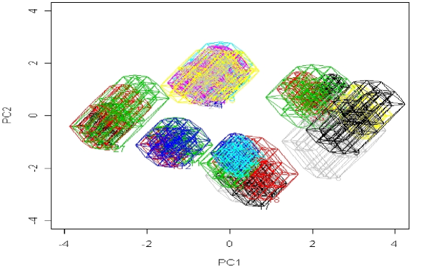
Figure 1: Faces Data - $PC_{1}~{}\times PC_{2}$ Polytopes

Figure 2 shows the corresponding principal component plots from these data when methods using the centers and /or ranges (or equivalently the end-points, i.e., vertices of the intervals) are used. Figure 2(a) (from Douzal et al., 2011, Fig. 6) shows the plots based on the vertices (interval end-points); Figure 2(b) (from Douzal et al., 2011, Fig. 9) shows the plots when the ranges are used; and Figure 2(c) (from Le-Rademacher and Billard, 2012, Figure 5(a)) results from using the Lauro and Palumbo (2000) range-transformation method. These three methods all use classical surrogates in their varying ways. Comparing the plots in Figure 2 with that of Figure 1, we can see that these approaches cannot correctly classify the faces. This is particularly evident when comparing Figure 2(b) with Figure 1 in light of the additional knowledge that the faces are actually nine sets of three measurements from each of nine persons. We observe that the three faces (rom1, rom2, rom3, e.g.) in Figure 2(b) are not clustered, as they are in Figure 1; likewise, for some other faces, the classical approaches do not necessarily form the 3-wise clusters as would be expected.

Details of the associated analytic diagnostics (such as inertia, etc.) including interpretations along with comparisons with PCA methodology based on classical surrogates can be found in Le-Rademacher and Billard (2012).

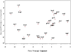
(a)	(b)
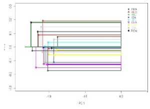
(c)

Figure 2: Faces Data - $PC_{1}~{}\times PC_{2}$ - (a) Vertices (b) Ranges (c) Range transformation

8 Conclusion

The initial theoretical work on deriving maximum likelihood (ML) estimators of parameters for interval data was that of Le-Rademacher and Billard (2011). Though important, their results were limited to obtaining MLE estimators for the mean and variance of a single interval-valued variable. However, the covariance statistic is a basic requirement for many methodologies (not just for standard data but also for interval data), including in particular regression analysis, principal component analysis, canonical correlation analysis, among others. Therefore, in this paper we have redressed the Le-Rademacher and Billard limitation by extending their results to deriving the MLEs for the core descriptive statistics for the two-dimensional case needed in these methodologies. The proposed MLE estimation approach can be developed for $p>2$-dimensional interval-valued variables by employing a $p$-dimensional normal distribution for the internal means, i.e., $\bm{\Theta}_{i1}$, and a $p$-variate Wishart distribution for the internal variations, i.e., $\bm{\Theta}_{i2}$, in the proposed likelihood function. The Le-Rademacher and Billard results emerge as special cases of our wider derivations. Asymptotic properties of the proposed maximum likelihood estimators are also derived.

Appendix A

Early work on interval data sometimes transformed the interval-valued variable into two variables, center and range (or, given their one-to-one correspondence equivalently into the end point values). Consider the $Y$ values of the interval-valued data sets of Table 3. Let us denote the interval centers by $Y^{c}=(a+b)/2$, and the interval half-range by $Y^{r}=(b-a)/2$. Then the first and second columns of Table 4(a) give the sample variances of $Y$ for the interval centers and ranges, respectively (calculated by classical results or as special cases of Eq.(2)). The third column shows the sum $(\mbox{Var}(Y^{c})+\mbox{Var}(Y^{r}))$. This can be compared with the sample variance $\mbox{Var}(Y)$ of the intervals in the right-most column (from Eq.(2) and Bertrand and Goupil, 2000). Thus we see that sometimes the sum $(\mbox{Var}(Y^{c})+\mbox{Var}(Y^{r}))$ is greater, and sometimes less, than the symbolic variance $\mbox{Var}(Y)$; this depends on the actual data. The fourth data set consists of classical values (with $a\equiv[a,a]$); in this case, the $\mbox{Var}(Y^{r})=0$ and so $\mbox{Var}(Y^{c})=\mbox{Var}(Y)$, as it should.

Table 3: Some Data Sets ($Y,X$)

Data Sets
1		2		3		4
$Y$	$X$	$Y$	$X$	$Y$	$X$	$Y$	$X$
[6,7]	[1,4]	[6,12]	[3,7]	[3,4]	[5,9]	[3, 3]	[4,4]
$[6,9]$	$[2,7]$	$[3,15]$	$[1,8]$	$[1,6]$	$[4,8]$	$[6,6]$	$[5,5]$
$[5,8]$	$[1,5]$	$[3,22]$	$[2,15]$	$[2,5]$	$[4,10]$	$[5,5]$	$[3,3]$
				[2,4]	[3,7]

Likewise, by using the centers and range values for both $Y$ and $X$, we can calculate the classical covariances of the centers and of the ranges and the symbolic interval covariances, from Eq.(3), shown in Table 4(b). Again, the sum $(\mbox{Cov}(Y^{c},X^{c})+\mbox{Cov}(Y^{r},X^{r}))$ can be greater, or smaller, than the symbolic covariance $\mbox{Cov}(Y,X)$; and for classical observations, this sum equals the symbolic covariance correctly as expected.

Table 4: Variances and Covariances

	(a) - Variances $Y$
Set	$\mbox{Var}(Y^{c})$	$\mbox{Var}(Y^{r})$	$\mbox{Var}(Y^{c})+\mbox{Var}(Y^{r})$	$\mbox{Var}(Y)$
1	0.222	0.889	1.111	0.750
2	2.722	28.222	30.944	17.750
3	0.047	2.188	2.234	0.859
4	1.556	0.000	1.556	1.556
	(b) - Covariances ($Y,X)$
Set	$\mbox{Cov}(Y^{c},X^{c})$	$\mbox{Cov}(Y^{r},X^{r})$	$\mbox{Cov}(Y^{c},X^{c})+\mbox{Cov}(Y^{r},X^{r})$	$\mbox{Cov}(Y,X)$
1	0.389	0.667	1.056	1.222
2	2.917	19.667	22.583	12.778
3	0.156	0.125	0.281	1.198
4	0.333	0.000	0.333	0.333

For a second aspect, suppose a data set consists of intervals all with the same center but different range values. Then, the variance-covariance terms for the centers are zero; and in contrast, if the data are such that the observations have different center values but all have the same range value, then the variance-covariance terms for the ranges are zero. Then for methods that rely on the relevant variance-covariance matrices, the methodology cannot be properly implemented, since, e.g., in regression that matrix is zero and for principal components the eigenvalues are zero.

The variance-covariance definition of Eq.(3) does not have these limitations.

Appendix B

The log likelihood function $\ln L_{I}$ from Eq.(12) and Eq.(4.1) is

$$\ln L_{I} \propto-n\ln(\sigma_{x})-n\ln(\sigma_{y})-(n/2)\ln(1-\rho^{2})$$

$$~{}~{}~{}-\frac{1}{2(1-\rho^{2})}\sum_{i=1}^{n}\bigg{[}\frac{\left(\theta_{i1}^{x}-\mu_{x}\right)^{2}}{\sigma^{2}_{x}}+\frac{\left(\theta_{i1}^{y}-\mu_{y}\right)^{2}}{\sigma^{2}_{y}}-2\rho\frac{(\theta_{i1}^{x}-\mu_{x})(\theta_{i1}^{y}-\mu_{y})}{\sigma_{x}\sigma_{y}}\bigg{]}$$

$$~{}~{}~{}-\frac{n\nu}{2}\ln\left(\gamma_{1}\gamma_{2}-\gamma_{3}^{2}\right)-\frac{\gamma_{1}\gamma_{2}}{2(\gamma_{1}\gamma_{2}-\gamma_{3}^{2})}\left(\frac{1}{\gamma_{1}}\sum_{i=1}^{n}\theta_{i2}^{x}+\frac{1}{\gamma_{2}}\sum_{i=1}^{n}\theta_{i2}^{y}-\frac{2\gamma_{3}}{\gamma_{1}\gamma_{2}}\sum_{i=1}^{n}\theta_{i2}^{xy}\right)$$

Then successively differentiating $\ln L_{I}$ with respect to each of the eight parameters in $\tau$, we obtain

$$\frac{\partial\ln L_{I}}{\partial\mu_{x}} =\frac{1}{(1-\rho^{2})}\left(\frac{1}{\sigma^{2}_{x}}\sum_{i=1}^{n}\left(\theta_{i1}^{x}-\mu_{x}\right)-\frac{\rho}{\sigma_{x}\sigma_{y}}\sum_{i=1}^{n}\left(\theta_{i1}^{y}-\mu_{y}\right)\right),$$

$$\frac{\partial\ln L_{I}}{\partial\mu_{y}} =\frac{1}{(1-\rho^{2})}\left(\frac{1}{\sigma^{2}_{y}}\sum_{i=1}^{n}\left(\theta_{i1}^{y}-\mu_{y}\right)-\frac{\rho}{\sigma_{x}\sigma_{y}}\sum_{i=1}^{n}\left(\theta_{i1}^{x}-\mu_{x}\right)\right),$$

$$\frac{\partial\ln L_{I}}{\partial\sigma_{x}} =\frac{-n}{\sigma_{x}}+\frac{1}{2(1-\rho^{2})}\left(\sum_{i=1}^{n}\frac{2\left(\theta_{i1}^{x}-\mu_{x}\right)^{2}}{\sigma^{3}_{x}}-2\rho\sum_{i=1}^{n}\frac{\left(\theta_{i1}^{x}-\mu_{x}\right)\left(\theta_{i1}^{y}-\mu_{y}\right)}{\sigma_{x}^{2}\sigma_{y}}\right),$$

$$\frac{\partial\ln L_{I}}{\partial\sigma_{y}} =\frac{-n}{\sigma_{y}}+\frac{1}{2(1-\rho^{2})}\left(\sum_{i=1}^{n}\frac{2\left(\theta_{i1}^{y}-\mu_{y}\right)^{2}}{\sigma^{3}_{y}}-2\rho\sum_{i=1}^{n}\frac{\left(\theta_{i1}^{x}-\mu_{x}\right)\left(\theta_{i1}^{y}-\mu_{y}\right)}{\sigma_{x}\sigma_{y}^{2}}\right),$$

$$\frac{\partial\ln L_{I}}{\partial\rho} =\frac{n\rho}{(1-\rho^{2})}-\frac{\rho}{(1-\rho^{2})^{2}}\left(\sum_{i=1}^{n}\frac{\left(\theta_{i1}^{x}-\mu_{x}\right)^{2}}{\sigma^{2}_{x}}+\sum_{i=1}^{n}\frac{\left(\theta_{i1}^{y}-\mu_{y}\right)^{2}}{\sigma^{2}_{y}}\right)$$

$$~{}~{}~{}~{}~{}~{}~{}~{}~{}~{}~{}~{}~{}~{}~{}~{}~{}~{}~{}~{}~{}~{}~{}~{}~{}~{}~{}~{}~{}~{}~{}~{}~{}~{}~{}~{}~{}+\frac{1+\rho^{2}}{(1-\rho^{2})^{2}}\sum_{i=1}^{n}\frac{(\theta_{i1}^{x}-\mu_{x})(\theta_{i1}^{y}-\mu_{y})}{\sigma_{x}\sigma_{y}},$$ (42)

$$\frac{\partial\ln L_{I}}{\partial\gamma_{1}} =-\frac{n\nu\gamma_{2}}{2G}+\frac{\gamma_{2}^{2}}{2G^{2}}\sum_{i=1}^{n}\theta_{i2}^{x}-\frac{G-\gamma_{1}\gamma_{2}}{2G^{2}}\sum_{i=1}^{n}\theta_{i2}^{y}-\frac{\gamma_{2}\gamma_{3}}{G^{2}}\sum_{i=1}^{n}\theta_{i2}^{xy},$$

$$\frac{\partial\ln L_{I}}{\partial\gamma_{2}} =-\frac{n\nu\gamma_{1}}{2G}-\frac{G-\gamma_{1}\gamma_{2}}{2G^{2}}\sum_{i=1}^{n}\theta_{i2}^{x}+\frac{\gamma_{1}^{2}}{2G^{2}}\sum_{i=1}^{n}\theta_{i2}^{y}-\frac{\gamma_{1}\gamma_{3}}{G^{2}}\sum_{i=1}^{n}\theta_{i2}^{xy},$$

$$\frac{\partial\ln L_{I}}{\partial\gamma_{3}} =\frac{n\nu\gamma_{3}}{G}-\frac{\gamma_{2}\gamma_{3}}{G^{2}}\sum_{i=1}^{n}\theta_{i2}^{x}-\frac{\gamma_{1}\gamma_{3}}{G^{2}}\sum_{i=1}^{n}\theta_{i2}^{y}+\frac{G+2\gamma_{3}^{2}}{G^{2}}\sum_{i=1}^{n}\theta_{i2}^{xy}$$

where $G=\gamma_{1}\gamma_{2}-\gamma_{3}^{2}$.

Then, substituting the relevant maximum likelihood estimator and setting the derivatives to zero, we can obtain the maximum likelihood estimators $\hat{\mbox{\boldmath$\tau$}}_{xy}=(\hat{\mu}_{x},\hat{\mu}_{y},\hat{\sigma}_{x}^{2},\hat{\sigma}_{y}^{2},\hat{\rho},\hat{\gamma}_{1},\hat{\gamma}_{2},\hat{\gamma}_{3})$ for $\mbox{\boldmath$\tau$}_{xy}=(\mu_{x},\mu_{y},\sigma_{x}^{2},\sigma_{y}^{2},\rho,\gamma_{1},\gamma_{2},\gamma_{3})$ to be as given by Eq.(19)-Eq.(22). We also note that instead of solving the partial derivative in Eq.(42) for the derivation of the estimator $\hat{\rho}$, we can more easily obtain the result of Eq.(42) by following, e.g., Casella and Berger (2002, p.358) who suggest using a partially maximized likelihood function.

References

References

- [1] Anderson, T. (2003). An Introduction to Multivariate Statistical Analysis, John Wiley.
- [2] Beranger, B., Lin, H. and Sisson S. A. (2022). New models for symbolic data analysis. Advances in Data Analysis and Classification 16.
- [3] Bertrand, P. and Goupil, F. (2000). Descriptive statistics for symbolic data. In: Analysis of Symbolic Data: Exploratory Methods for Extracting Statistical Information from Complex Data (Eds. H.-H. Bock and E. Diday), 103-124. Springer-Verlag, Berlin.
- [4] Billard, L. (2008). Sample covariance functions for complex quantitative data. In: World Congress, International Association of Computational Statistics (Eds. M. Mizuta and J. Nakano), 157-163. Japanese Society of Computational Statistics, Yokohama, Japan.
- [5] Billard, L. and Diday, E. (2003). From the statistics of data to the statistics of knowledge: Symbolic data analysis. Journal of the American Statistical Association 98, 470-487.
- [6] Billard, L. and Diday, E. (2006). Symbolic Data Analysis: Conceptual Statistics and Data Mining. Wiley, Chichester.
- [7] Bock, H.-H. and Diday, E. (Editors) (2000). Analysis of Symbolic Data: Exploratory Methods for Extracting Statistical Information from Complex Data. Springer-Verlag, Berlin.
- [8] Brito, P. and Polaillon, G. (2005). Structuring probabilist data by Galois lattices. Mathematics and Social Sciences 43, 77-104.
- [9] Cariou, V. and Billard, L. (2015). Generalization method when manipulating relational databases. Revue des Nouvelles Technologies de l’Information 27, 59-86.
- [10] Casella, G. and Berger, R. L. (2002). Statistical Inference, 2nd Edition. Pacific Grove CA: Duxbury.
- [11] Clark, C. E. (1962). The PERT model for the distribution of activity time. Operations Research 10, 405-406.
- [12] Diday, E. (1988). The symbolic approach in clustering and related methods of data analysis. In: Classification and Related Methods of Data Analysis, Proceeding IFCS 1987 (Aachen, Germany) (Ed. H.-H. Bock), 673-684, North-Holland.
- [13] Diday, E. (1995). Probabilist, possibilist and belief objects for knowledge analysis. Annals of Operations Research 55, 227-276.
- [14] Diday, E. and Emilion, R. (1996). Lattices and capacities in analysis of probabilist objects. In: Ordinal and Symbolic Data, Proceeding International Conference on Ordinal and Symbolic Data Analysis - OSDA 95, Paris (Eds. E. Diday, Y. Lechevallier, O. Opitz), 13-30, Springer, Heidelberg.
- [15] Diday, E. and Emilion, R. (1998). Capacities and credibilities in analysis of probabilistic objects by histograms and lattices. In: Data Science, Classification, and Related Methods (Eds. C. Hayashi, N. Obsumi, K. Yajima, Y. Tanaka, H.-H. Bock and Y. Baba), 353-357, Springer.
- [16] Diday, E. and Emilion, R. (2003). Maximal and stochastic Galois lattices. Discrete Applied Mathematics 127, 271-284.
- [17] Diday, E., Emilion, R. and Hillali, Y. (1996). Symbolic data analysis of probabilistic objects by capacities and credibilities. Proc. XXXVIII Riunione Scientifica Societ Italiana di Statistica, 5-22.
- [18] Douzal-Chouakria, A., Billard, L. and Diday, E. (2011). Principal component analysis for interval-valued observations. Statistical Analysis and Data Mining 4, 229-246.
- [19] Emilion, R. (1997). Diffrentiation des capacits et des intgrales de Choquet. Comptes Rendus de l’Academie des Sciences - Series I - Mathematics 324, 389-392.
- [20] Fisher, R. A. (1915). Frequency distribution of the values of the correlation coefficient in samples from an indefinitely large population. Biometrika 10, 507-521.
- [21] Lauro, N. C. and Palumbo, F. (2000). Principal component analysis of interval data: A symbolic data analysis approach. Computational Statistics 15, 73-87.
- [22] Lehmann, E. L. (1983). Theory of Point Estimation. Wiley-Interscience.
- [23] Lehmann, E. L. (1986). Testing Statistical Hypotheses. 2nd Edition. Wiley-Interscience.
- [24] Le-Rademacher, J. and Billard, L. (2011). Likelihood functions and some maximum likelihood estimators for symbolic data. Journal of Statistical Inference and Planning 141, 1593-1602.
- [25] Le-Rademacher, J. and Billard, L. (2012). Symbolic-covariance principal component analysis and visualization for interval-valued data. Journal of Computational and Graphical Statistics 21, 413-432.
- [26] Leroy, B., Chouakria, A., Herlin, I. and Diday, E. (1996). Approche géométrique et classification pour la reconnaissance de visage. Reconnaissance des Forms et Intelligence Artificelle, INRIA and IRISA and CNRS, France, p 548-557.
- [27] Liu, F. and Billard, L. (2022). Partition of interval-valued observations using regression. Journal of Classification 39, 55-77.
- [28] Malcolm, D. G., Roseboom, J. H., Clark, C. E. and Fazar, W. (1959). Application of a technique for research and development program evaluation. Operations Research 7, 646-669.
- [29] Moore, R. E. (1966) Interval Analysis. Prentice-Hall. Englewood Cliffs NJ.
- [30] Oliveira, M. R., Azeitona, M., Pacheco, A. and Valadas, R. (2022). Association measures for interval variables. Advances in Data Analysis and Classification 16, 491-520.
- [31] Oliveira, M. R., Vilela, M., Pacheco, A., Valadas, R. and Salvador, P. (2017). Extracting information from interval data using symbolic principal component analysis. Austrian Journal of Statistics 46, 79-87.
- [32] Rahman, P. A., Beranger, B., Roughan, M. and Sisson S. A. (2020). Likelihood-based inference for modelling packet transit from thinned flow summaries. IEEE Transactions on Signal and Information Processing over Networks 8, 571-583.
- [33] Samadi, S. Y. and Billard, L. (2021). Analysis of dependent data aggregated into intervals. Journal of Multivariate Analysis 186, 104817.
- [34] Wishart, J. (1928). The generalised product moment distribution distribution in samples from a normal multivariate population. Biometrika 20, 32-52.
- [35] Whitaker, T., Beranger, B. and Sisson S. A. (2020). Composite likelihood methods for histogram-valued random variables. Statistics and Computing 30, 1459-1477.
- [36] Whitaker, Beranger, T., B. and Sisson S. A. (2021). Logistic regression models for aggregated data. Journal of Computational and Graphical Statistics 30, 1049-1067.
- [37] Xu, W. (2010). Symbolic Data Analysis: Interval-Valued Data Regression. Doctoral Dissertation, University of Georgia.
- [38] Zhang, X., Beranger, B. and Sisson S. A. (2020). Constructing likelihood functions for interval-valued random variables. Scandinavian Journal of Statistics 47, 1-35.