XGrad: Boosting Gradient-Based Optimizers With Weight Prediction

Abstract

In this paper, we propose a general deep learning training framework XGrad which introduces weight prediction into the popular gradient-based optimizers to boost their convergence and generalization when training the deep neural network (DNN) models. In particular, ahead of each mini-batch training, the future weights are predicted according to the update rule of the used optimizer and are then applied to both the forward pass and backward propagation. In this way, during the whole training period, the optimizer always utilizes the gradients w.r.t. the future weights to update the DNN parameters, making the gradient-based optimizer achieve better convergence and generalization compared to the original optimizer without weight prediction. XGrad is rather straightforward to implement yet pretty effective in boosting the convergence of gradient-based optimizers and the accuracy of DNN models. Empirical results concerning the most three popular gradient-based optimizers including SGD with momentum, Adam, and AdamW demonstrate the effectiveness of our proposal. The experimental results validate that XGrad can attain higher model accuracy than the original optimizers when training the DNN models. The code of XGrad will be available at: https://github.com/guanleics/XGrad.

I Introduction

The training of deep neural network (DNN) models is to find the optimal parameters using an optimizer which has a decisive influence on the accuracy of the models. The gradient-based optimization methods are currently of core practical importance in deep learning as they can attain rapid training of modern deep neural network models. Among all gradient-based optimizers, stochastic gradient descent (SGD) with momentum [1, 2] and adaptive methods such as Adam [3] and AdamW [4] are the most popular optimizers and have become the default choices for training many DNN models include convolutional neural networks (CNN) [5, 6, 7, 8], recurrent neural networks (RNN), graph neural networks (GNN) [9, 10, 11], generative adversarial networks (GAN) [12] and lots of transformer-based DNN models such as Transformer [13], Bert [14], Vision Transformer [15, 16] and GPT-2/3 [17, 18], etc.

When training a DNN model using the gradient-based optimizers, each mini-batch training generally consists of one forward pass and one backward propagation, where the gradients w.r.t. all the parameters (also known as weights) are computed during the backward propagation. After that, the generated gradients are utilized by the optimizer to calculate the update values for all parameters, which are finally applied to updating the DNN weights. We exemplify this using the training process of mini-batch SGD [19]. We assume that the mini-batch size is $b$, the neural network weights at step $t$ are $\bm{\theta}_{t}$, and the loss function is $f(\cdot)$. In each iteration, given a mini-batch training data $({\bf x}_{i},{\bf y}_{i})$, the forward pass first computes the loss with ${\bf z}_{i}=f({\bm{\theta}}_{t},{\bf x}_{i},{\bf y}_{i})$. Then, the gradients generated in the backward propagation can be calculated as

$${\bf g}_{t}=\frac{1}{b}\sum_{i=1}^{b}\nabla_{\bm{\theta}}f({\bm{\theta}}_{t},{\bf z}_{i}).$$ (1)

After that, given the learning rate $\gamma_{t}$, the DNN weights are updated via

$${\bm{\theta}}_{t+1}={\bm{\theta}}_{t}-\gamma_{t}{\bf g}_{t}.$$ (2)

For gradient-based optimization methods, the differences among different optimization methods lie in that the ways using the gradients generated by (1) to update model parameters are different. To be general, the weights are updated by $\bm{\theta}_{t+1}\leftarrow\bm{\theta}_{t}+\Delta\bm{\theta}_{t}$, where $\Delta\bm{\theta}_{t}$ denotes the relative increments of $\bm{\theta}_{t+1}$ over $\bm{\theta}_{t}$ computed by the specific optimizer. Figure 1 illustrates the optimization of DNN weights. The remarkable features of existing gradient-based optimizers can be summarized as follows. First, the updates of weights are continuous. Second, each mini-batch uses the currently available weights to do both forward pass and backward propagation. Third, in comparison with the current weights, the updated weights tend to be closer to the optimal point. In other words, in each mini-batch training, the weights tend to be updated in a “correct” direction to move towards the optimal point.

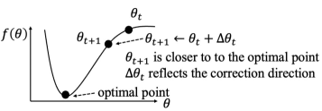
Figure 1: The optimization of DNN weights.

Motivated by the fact that DNN weights are updated in a continuous manner and the update values calculated by each gradient-based optimizer should reflect the “correct” direction for updating the weights, we introduce weight prediction [20, 21] into the DNN training and, in particular, propose a general framework XGrad to boost the convergence of gradient-based optimizers and to improve the accuracy of DNN models. The XGrad framework is not only very straightforward to implement but also well suited for a large class of gradient-based optimization methods including SGD with momentum, AdaGrad [22], RMSprop [23], Adam, AdamW, etc. Previously, we explored weight prediction for DNN training in a short conference paper [24] where we introduced weight prediction into the DNN training when using AdamW [4] as an optimizer. In this paper, we study weight prediction in detail and enable it to cover a large class of gradient-based optimizers including SGD with momentum and adaptive methods such as AdaGrad, RMSprop, Adam, AdamW, and so on. Concretely, in each mini-batch training, XGrad consists of the following three steps: 1) Ahead of the forward pass, cache the current weights and predict the future weights according to the specific update rule of the used gradient-based optimizer. 2) Use the predicted weights to perform both the forward pass and backward propagation after which the gradients w.r.t. the parameters of each layer are generated. 3) Recover the cached weights and then update all parameters with the newly generated gradients.

We conduct extensive experiments to validate the effectiveness of our proposal. The experiment results demonstrate that XGrad can improve the model accuracy compared with the original optimizer. For example, when training on CIFAR-10 and CIFAR-100 datasets, XGrad respectively leads to an average of 0.89% and 2.92% top-1 accuracy improvement over the SGD with momentum optimizer. On the image classification task, XGrad also averagely yields 1.28% and 1.0% accuracy improvement over Adam and AdamW, respectively.

The contributions of this paper can be summarized as follows:

• We, for the first time, construct the mathematical relationship between currently available weights and future weights after several continuous updates when using the most popular gradient-based optimizers including SGD with momentum, RMSprop, AdaGrad, Adam, AdamW, etc.

• We devise a general workflow for incorporating weight prediction into the DNN training. To the best of our knowledge, this is the first time that applies weight prediction strategy to boost the convergence and generalization of popular gradient-based optimizers.

• We conducted extensive experimental evaluations to validate the effectiveness of our proposal by using the three most popular optimizers: SGD with momentum, Adam, and AdamW. The experiment results demonstrate that our proposal works well for both SGD and adaptive gradient methods such as Adam and AdamW.

The rest of this paper is organized as follows: Section II briefly presents the related research work about gradient-based optimizers. Section III lays the foundation of weight prediction where we build up the mathematical relationship between the initial weights and the future weights after $s$ continuous updates when using SGD with momentum, RMSprop, AdaGrad, Adam, and AdamW. Section IV further constructs the XGrad framework on the basis of Section III. Extensive experiments are conducted in Section V to validate the effectiveness of our proposal. Finally, we conclude this paper and discuss the future work in Section VI.

II Related Work

The research on optimization methods always remains a hotspot in the field of deep learning as the convergence trait of the used optimizer directly affects convergence and the accuracy of the model. Generally, the training procedure of a DNN model is built upon backpropagation [25] where each layer of neural network weights is fine-tuned along the backward propagation of “errors”. Backpropagation always comes along with gradient descent. Currently, first-order gradient methods, such as SGD with momentum [2] and adaptive methods [26, 3, 27] are the most widely used deep learning optimization methods.

Typically, gradient descent (GD) requires to use all training samples to calculate the gradients at each iteration. It is seldom used in deep learning because of the expensive calculation. Mini-batch SGD can remarkably decrease the per-iteration calculation cost. When using mini-batch SGD, one needs to randomly sample a mini-batch of training instances, then calculate the gradients, and finally update the weights. This not only ensures low per-iteration computational cost but also conserves the randomness and the stability of gradient descent. To further boost the convergence trait of SGD, Qian et al. [1] introduced the momentum term and proposed SGD with momentum. The momentum in each iteration is the weighted average of the momentum from the last iteration and the gradients at this iteration. The momentum term accumulates the gradient information from all previous iterations, making the weights parameter update along the way of inertia directions. Presently, SGD with momentum has been regarded as the default optimizer especially for image classification tasks [5, 6, 7, 8]. Another noteworthy feature of SGD with momentum is that a unified learning rate for all parameters is used throughout the entire training period.

Noticing that the learning rate plays a significant role in DNN training, many researchers turn to studying adaptive methods (also known as adaptive learning methods), which compute a specific learning rate for each individual parameter. In 2011, Duchi et al. [22] proposed AdaGrad, which dynamically adjusts the learning rate according to the history gradients from previous iterations and utilizes the quadratic sum of all previous gradients to update the model parameters. Zeiler [26] proposed AdaDelta, seeking to alleviate the continual decay of the learning rate of AdaGrad. AdaDelta does not require manual tuning of a learning rate and is robust to noisy gradient information. Tieleman and Hinton [23] refined AdaGrad and proposed RMSprop. The same as AdaGrad, RMSprop adjusts the learning rate via element-wise computation and then updates the variables. One remarkable feature of RMSprop is that it can avoid decaying the learning rate too quickly. In order to combine the advantages of both AdaGrad and RMSprop, Kingma and Ba [3] proposed another famous adaptive gradient method, Adam, which has become the most important choice for training many Transformer-based DNN models [23, 3, 4]. Loshchilov and Hutter [4] found that the major factor of the poor generalization of Adam is due to that $L_{2}$ regularization for it is not as effective as for its competitor, i.e., SGD with momentum. They further proposed decoupled weight decay regularization for Adam, which is also known as AdamW. The experimental results demonstrate that AdamW substantially improves the generalization performance of Adam and illustrates competitive performance as SGD with momentum [2] when tackling image classification tasks. Currently, Adam as well as AdamW have become the default optimizer for DNN training. To simultaneously achieve fast convergence and good generalization, Zhuang et al. [27] proposed another adaptive gradient method called AdaBelief, which adapts the stepsize according to the “belief” in the current gradient direction. Other proposed adaptive methods include Yogi [28], AdaBound [29], RAdam [30], etc. Noticing that the second-moment estimation of Adam is a more favorable option for learning rate scaling than that of the raw gradient, Wang et al. [31] proposed AdaMomentum. Reddi et al. [32] studied why RMSProp and Adam probably do not converge to an optimal solution and proposed a new exponential moving average variant: AMSGrad. Considering that Nesterov’s accelerated gradient [33] has a better bound than gradient descent, Timothy Dozat incorporated Nestorv momentum into Adam and proposed a new optimization method named NAdam [34]. Chen et al. [35] studied the convergence of adaptive gradient methods including these popular algorithms such as Adam, AMSGrad, and AdaGrad.

Notably, SGD with momentum as well as all adaptive methods share a common feature: weight updates are performed in a continuous manner and each mini-batch training always utilizes currently available weights to do both forward pass and backward propagation. Weight prediction was previously used to overcome the weight inconsistency issue in the asynchronous pipeline parallelism. Chen et al. [21] used the smoothed gradient to replace the true gradient in order to predict future weights when using SGD with momentum [2] as the optimizer. Guan et al. [20] proposed using the update values of Adam [3] to perform weight predictions. Yet, both approaches use weight prediction to ensure effective parameter learning in the asynchronous pipeline training rather than considering the impact of weight prediction on the optimizers themselves.

III Gradient-based Optimizers

In this section, we construct the mathematical relationship between the initial weights (denoted as ${\bm{\theta}}_{0}$) and the future weights after $s$ ($s>1$) times of continuous updates (dubbed as ${{\bm{\theta}}_{s}}$) when training the DNN models using gradient-based optimizers such as SGD with momentum, AdaGrad, RMSprop, Adam and AdamW.

Ahead of any $t$-th ($t\geq 1$) iteration, we assume that the current available DNN weights are ${\bm{\theta}}_{t-1}$. Throughout this paper, we always let $\gamma$ ($\gamma\in\mathbb{R}$) denote the learning rate and refer to $\lambda$ ($\lambda\in\mathbb{R}$) as the weight decay.

III-A SGD with momentum

We first reformulate the update of SGD with momentum as

$${\bm{\theta}}_{t}={\bm{\theta}}_{t-1}-\gamma\cdot{\bf v}_{t},$$ (3)

s.t. $$\left\{\begin{array}[]{ll}\mathbf{g}_{t}=\nabla_{\bm{\theta}}f_{t}({\bm{\theta}}_{t-1}),\\ \mathbf{g}_{t}=\mathbf{g}_{t}+\lambda{\bm{\theta}}_{t-1},\\ {\mathbf{v}}_{t}=u\cdot\mathbf{v}_{t-1}+(1-\tau)\cdot\mathbf{g}_{t}.\end{array}\right.$$

where $u$ is the momentum factor and $\tau$ is the dampening for momentum.

Letting ${\bm{\theta}}_{0}$ denote the initial weights of a DNN model, then in the following $s$ times of continuous mini-batch training, the DNN weights are updated via

$${\bm{\theta}}_{1}={\bm{\theta}}_{0}-\gamma\cdot{\bf v}_{1},$$ (4)

$${\bm{\theta}}_{2}={\bm{\theta}}_{1}-\gamma\cdot{\bf v}_{2},$$

$$\cdots$$

$${\bm{\theta}}_{s}={\bm{\theta}}_{s-1}-\gamma\cdot{\bf v}_{s},$$

where for any $i\in\{1,2,\cdots,s\}$, we have

$$\left\{\begin{array}[]{ll}\mathbf{g}_{i}=\nabla_{\bm{\theta}}f_{i}({\bm{\theta}}_{i-1}),\\ \mathbf{g}_{i}=\mathbf{g}_{i}+\lambda{\bm{\theta}}_{i-1},\\ \mathbf{v}_{i}=u\cdot\mathbf{v}_{i-1}+(1-\tau)\cdot\mathbf{g}_{i}.\\ \end{array}\right.$$ (5)

When summing up all weight update equations in (4), we have

$${\bm{\theta}}_{s}={\bm{\theta}}_{0}-\gamma\sum_{i=1}^{s}{\bf v}_{i},$$ (6)

s.t. $$\left\{\begin{array}[]{ll}\mathbf{g}_{i}=\nabla_{\bm{\theta}}f_{i}({\bm{\theta}}_{i-1}),\\ \mathbf{g}_{i}=\mathbf{g}_{i}+\lambda{\bm{\theta}}_{i-1},\\ \mathbf{v}_{i}=u\cdot\mathbf{v}_{i-1}+(1-\tau)\cdot\mathbf{g}_{i}.\\ \end{array}\right.$$

III-B AdaGrad

We reformulate the update of AdaGrad as

$${\bm{\theta}}_{t}={\bm{\theta}}_{t-1}-\frac{\gamma\cdot{\bf g}_{t}}{(1+(t-1)\eta)\cdot(\sqrt{{\bf v}_{t}}+\epsilon)},$$ (7)

s.t. $$\left\{\begin{array}[]{ll}\mathbf{g}_{t}=\nabla_{\bm{\theta}}f_{t}({\bm{\theta}}_{t-1}),\\ \mathbf{g}_{t}=\mathbf{g}_{t}+\lambda{\bm{\theta}}_{t-1},\\ \mathbf{v}_{t}=\mathbf{v}_{t-1}+\mathbf{g}_{t}^{2},\\ \end{array}\right.$$

where $\eta$ is the learning rate decay and $\epsilon$ (default: $1e^{-10}$) is used to improve numerical stability.

The DNN weights are updated via

$${\bm{\theta}}_{1}={\bm{\theta}}_{0}-\frac{\gamma\cdot{\bf g}_{1}}{(1+(1-1)\eta)\cdot(\sqrt{{\bf v}_{1}}+\epsilon)},$$ (8)

$${\bm{\theta}}_{2}={\bm{\theta}}_{1}-\frac{\gamma\cdot{\bf g}_{2}}{(1+(2-1)\eta)\cdot(\sqrt{{\bf v}_{2}}+\epsilon)},$$

$$\cdots$$

$${\bm{\theta}}_{s}={\bm{\theta}}_{s-1}-\frac{\gamma\cdot{\bf g}_{s}}{(1+(s-1)\eta)\cdot(\sqrt{{\bf v}_{s}}+\epsilon)},$$

where for any $i\in\{1,2,\cdots,s\}$, we have

$$\left\{\begin{array}[]{ll}\mathbf{g}_{i}=\nabla_{\bm{\theta}}f_{i}({\bm{\theta}}_{i-1}),\\ \mathbf{g}_{i}=\mathbf{g}_{i}+\lambda{\bm{\theta}}_{i-1},\\ \mathbf{v}_{i}=\mathbf{v}_{i-1}+\mathbf{g}_{i}^{2}.\\ \end{array}\right.$$ (9)

Summing up all equations in (8) further yields

$${\bm{\theta}}_{s}={\bm{\theta}}_{0}-\sum_{i=1}^{s}\frac{\gamma\cdot{\bf g}_{i}}{(1+(i-1)\eta)\cdot(\sqrt{{\bf v}_{i}}+\epsilon)},$$ (10)

s.t. $$\left\{\begin{array}[]{ll}\mathbf{g}_{i}=\nabla_{\bm{\theta}}f_{i}({\bm{\theta}}_{i-1}),\\ \mathbf{g}_{i}=\mathbf{g}_{i}+\lambda{\bm{\theta}}_{i-1},\\ \mathbf{v}_{i}=\mathbf{v}_{i-1}+\mathbf{g}_{i}^{2}.\\ \end{array}\right.$$

III-C RMSprop

We reformulate the update of RMSprop as

$${\bm{\theta}}_{t}={\bm{\theta}}_{t-1}-\frac{\gamma\cdot{\bf g}_{t}}{\sqrt{{\bf v}_{t}}+\epsilon},$$ (11)

s.t. $$\left\{\begin{array}[]{ll}\mathbf{g}_{t}=\nabla_{\bm{\theta}}f_{t}({\bm{\theta}}_{t-1}),\\ \mathbf{v}_{t}=\alpha\cdot\mathbf{v}_{t-1}+(1-\alpha)\cdot\mathbf{g}_{t}^{2},\\ \end{array}\right.$$

where $a$ denotes the smoothing constant and $\epsilon$ (default: $1e^{-8}$) is used to improve numerical stability.

Likewise, during the first $s$ times of continuous mini-batch training, the DNN weights are updated via

$${\bm{\theta}}_{1}={\bm{\theta}}_{0}-\frac{\gamma\cdot{\bf g}_{1}}{\sqrt{{\bf v}_{1}}+\epsilon},$$ (12)

$${\bm{\theta}}_{2}={\bm{\theta}}_{1}-\frac{\gamma\cdot{\bf g}_{2}}{\sqrt{{\bf v}_{2}}+\epsilon},$$

$$\cdots$$

$${\bm{\theta}}_{s}={\bm{\theta}}_{s-1}-\frac{\gamma\cdot{\bf g}_{s}}{\sqrt{{\bf v}_{s}}+\epsilon},$$

where for any $i\in\{1,2,\cdots,s\}$, we have

$$\left\{\begin{array}[]{ll}\mathbf{g}_{i}=\nabla_{\bm{\theta}}f_{i}({\bm{\theta}}_{i-1}),\\ \mathbf{v}_{i}=\alpha\cdot\mathbf{v}_{i-1}+(1-\alpha)\cdot\mathbf{g}_{i}^{2}.\\ \end{array}\right.$$ (13)

When summing up all weight update equations in (12), we have

$${\bm{\theta}}_{s}={\bm{\theta}}_{0}-\sum_{i=1}^{s}\frac{\gamma\cdot{\bf g}_{i}}{\sqrt{{\bf v}_{i}}+\epsilon},$$ (14)

s.t. $$\left\{\begin{array}[]{ll}\mathbf{g}_{i}=\nabla_{\bm{\theta}}f_{i}({\bm{\theta}}_{i-1}),\\ \mathbf{v}_{i}=\alpha\cdot\mathbf{v}_{i-1}+(1-\alpha)\cdot\mathbf{g}_{i}^{2}.\\ \end{array}\right.$$

III-D Adam

We reformulate the update of Adam as

$${\bm{\theta}}_{t}={\bm{\theta}}_{t-1}-\frac{\gamma{\hat{\bf m}_{t}}}{\sqrt{\hat{\bf v}_{t}}+\epsilon},$$ (15)

s.t. $$\left\{\begin{array}[]{ll}\mathbf{g}_{t}=\nabla_{\bm{\theta}}f_{t}({\bm{\theta}}_{t-1}),\\ {\mathbf{m}}_{t}=\beta_{1}\cdot\mathbf{m}_{t-1}+(1-\beta_{1})\cdot\mathbf{g}_{t},\\ \mathbf{v}_{t}=\beta_{2}\cdot\mathbf{v}_{t-1}+(1-\beta_{2})\cdot\mathbf{g}_{t}^{2},\\ \hat{\mathbf{m}}_{t}=\frac{\mathbf{m}_{t}}{1-\beta_{1}^{t}},\\ \hat{\mathbf{v}}_{t}=\frac{\mathbf{v}_{t}}{1-\beta_{2}^{t}}.\end{array}\right.$$

In (15), ${\mathbf{m}}_{t}$ and ${\mathbf{v}}_{t}$ refer to the first and second moment vector respectively, $\beta_{1}$ and $\beta_{2}$ are coefficients used for computing ${\bf m}_{t}$ and ${\bf v}_{t}$ respectively, $\epsilon$ is the smoothing term that can prevent division by zero.

When training the DNN weights from ${\bm{\theta}}_{0}$, in the following $s$ times of continuous mini-batch training, the DNN weights are updated via

$${\bm{\theta}}_{1}={\bm{\theta}}_{0}-\frac{\gamma{\hat{\bf m}_{1}}}{\sqrt{\hat{\bf v}_{1}}+\epsilon},$$ (16)

$${\bm{\theta}}_{2}={\bm{\theta}}_{1}-\frac{\gamma{\hat{\bf m}_{2}}}{\sqrt{\hat{\bf v}_{2}}+\epsilon},$$

$$\cdots$$

$${\bm{\theta}}_{s}={\bm{\theta}}_{s-1}-\frac{\gamma{\hat{\bf m}_{s}}}{\sqrt{\hat{\bf v}_{s}}+\epsilon},$$

where for any $i\in\{1,2,\cdots,s\}$, we have

$$\left\{\begin{array}[]{ll}\mathbf{g}_{i}=\nabla_{\bm{\theta}}f_{i}({\bm{\theta}}_{i-1}),\\ {\mathbf{m}}_{i}=\beta_{1}\cdot\mathbf{m}_{i-1}+(1-\beta_{1})\cdot\mathbf{g}_{i},\\ \mathbf{v}_{i}=\beta_{2}\cdot\mathbf{v}_{i-1}+(1-\beta_{2})\cdot\mathbf{g}_{i}^{2},\\ \hat{\mathbf{m}}_{i}=\frac{\mathbf{m}_{i}}{1-\beta_{1}^{i}},\\ \hat{\mathbf{v}}_{i}=\frac{\mathbf{v}_{i}}{1-\beta_{2}^{i}}.\\ \end{array}\right.$$ (17)

When summing up all weight update equations in (16), we have

$${\bm{\theta}}_{s}={\bm{\theta}}_{0}-\sum_{i=1}^{s}\frac{\gamma\hat{\bf m}_{i}}{\sqrt{\hat{\bf v}_{i}}+\epsilon},$$ (18)

s.t. $$\left\{\begin{array}[]{ll}\mathbf{g}_{i}=\nabla_{\bm{\theta}}f_{i}({\bm{\theta}}_{i-1}),\\ {\mathbf{m}}_{i}=\beta_{1}\cdot\mathbf{m}_{i-1}+(1-\beta_{1})\cdot\mathbf{g}_{i},\\ \mathbf{v}_{i}=\beta_{2}\cdot\mathbf{v}_{i-1}+(1-\beta_{2})\cdot\mathbf{g}_{i}^{2},\\ \hat{\mathbf{m}}_{i}=\frac{\mathbf{m}_{i}}{1-\beta_{1}^{i}},\\ \hat{\mathbf{v}}_{i}=\frac{\mathbf{v}_{i}}{1-\beta_{2}^{i}}.\\ \end{array}\right.$$

III-E AdamW

Given the momentum factor $\beta_{1}\in\mathbb{R}$ and $\beta_{2}\in\mathbb{R}$, we reformulate the update of AdamW [4] as

$${\bm{\theta}}_{t}=(1-\gamma\lambda){\bm{\theta}}_{t-1}-\frac{\gamma{\hat{\bf m}_{t}}}{\sqrt{\hat{\bf v}_{t}}+\epsilon},$$ (19)

s.t. $$\left\{\begin{array}[]{ll}\mathbf{g}_{t}=\nabla_{\bm{\theta}}f_{t}({\bm{\theta}}_{t-1}),\\ {\mathbf{m}}_{t}=\beta_{1}\cdot\mathbf{m}_{t-1}+(1-\beta_{1})\cdot\mathbf{g}_{t},\\ \mathbf{v}_{t}=\beta_{2}\cdot\mathbf{v}_{t-1}+(1-\beta_{2})\cdot\mathbf{g}_{t}^{2},\\ \hat{\mathbf{m}}_{t}=\frac{\mathbf{m}_{t}}{1-\beta_{1}^{t}},\\ \hat{\mathbf{v}}_{t}=\frac{\mathbf{v}_{t}}{1-\beta_{2}^{t}}.\end{array}\right.$$

Likewise, the first $s$ times of continuous mini-batch training can be formulated as

$${\bm{\theta}}_{1}=(1-\gamma\lambda){\bm{\theta}}_{0}-\frac{\gamma{\hat{\bf m}_{1}}}{\sqrt{\hat{\bf v}_{1}}+\epsilon},$$ (20)

$${\bm{\theta}}_{2}=(1-\gamma\lambda){\bm{\theta}}_{1}-\frac{\gamma{\hat{\bf m}_{2}}}{\sqrt{\hat{\bf v}_{2}}+\epsilon},$$

$$\cdots$$

$${\bm{\theta}}_{s}=(1-\gamma\lambda){\bm{\theta}}_{s-1}-\frac{\gamma{\hat{\bf m}_{s}}}{\sqrt{\hat{\bf v}_{s}}+\epsilon},$$

where for any $i\in\{1,2,\cdots,s\}$, we have

$$\left\{\begin{array}[]{ll}\mathbf{g}_{i}=\nabla_{\bm{\theta}}f_{i}({\bm{\theta}}_{i-1}),\\ {\mathbf{m}}_{i}=\beta_{1}\cdot\mathbf{m}_{i-1}+(1-\beta_{1})\cdot\mathbf{g}_{i},\\ \mathbf{v}_{i}=\beta_{2}\cdot\mathbf{v}_{i-1}+(1-\beta_{2})\cdot\mathbf{g}_{i}^{2},\\ \hat{\mathbf{m}}_{i}=\frac{\mathbf{m}_{i}}{1-\beta_{1}^{i}},\\ \hat{\mathbf{v}}_{i}=\frac{\mathbf{v}_{i}}{1-\beta_{2}^{i}}.\\ \end{array}\right.$$ (21)

When summing up all weight update equations in (20), we have

$${\bm{\theta}}_{s}={\bm{\theta}}_{0}-\gamma\lambda\sum_{i=0}^{s-1}{\bm{\theta}}_{i}-\sum_{i=1}^{s}\frac{\gamma\hat{\bf m}_{i}}{\sqrt{\hat{\bf v}_{i}}+\epsilon},$$ (22)

s.t. $$\left\{\begin{array}[]{ll}\mathbf{g}_{i}=\nabla_{\bm{\theta}}f_{i}({\bm{\theta}}_{i-1}),\\ {\mathbf{m}}_{i}=\beta_{1}\cdot\mathbf{m}_{i-1}+(1-\beta_{1})\cdot\mathbf{g}_{i},\\ \mathbf{v}_{i}=\beta_{2}\cdot\mathbf{v}_{i-1}+(1-\beta_{2})\cdot\mathbf{g}_{i}^{2},\\ \hat{\mathbf{m}}_{i}=\frac{\mathbf{m}_{i}}{1-\beta_{1}^{i}},\\ \hat{\mathbf{v}}_{i}=\frac{\mathbf{v}_{i}}{1-\beta_{2}^{i}}.\\ \end{array}\right.$$

It is well known that the weight decay value $\lambda$ is generally set to an extremely small value (e.g., $5e^{-4}$), and the learning rate $\gamma$ is commonly set to a value smaller than 1 (e.g., $1e^{-3}$). Consequently, $\gamma\lambda$ is pretty close to zero, and thus, the second term of the right hand of (22) can be neglected. This, therefore, generates the following equation:

$${\bm{\theta}}_{s}\approx{\bm{\theta}}_{0}-\sum_{i=1}^{s}\frac{\gamma\hat{\bf m}_{i}}{\sqrt{\hat{\bf v}_{i}}+\epsilon}.$$ (23)

s.t. $$\left\{\begin{array}[]{ll}\mathbf{g}_{i}=\nabla_{\bm{\theta}}f_{i}({\bm{\theta}}_{i-1}),\\ {\mathbf{m}}_{i}=\beta_{1}\cdot\mathbf{m}_{i-1}+(1-\beta_{1})\cdot\mathbf{g}_{i},\\ \mathbf{v}_{i}=\beta_{2}\cdot\mathbf{v}_{i-1}+(1-\beta_{2})\cdot\mathbf{g}_{i}^{2},\\ \hat{\mathbf{m}}_{i}=\frac{\mathbf{m}_{i}}{1-\beta_{1}^{i}},\\ \hat{\mathbf{v}}_{i}=\frac{\mathbf{v}_{i}}{1-\beta_{2}^{i}}.\\ \end{array}\right.$$

IV The XGrad framework

When summarizing Equations (6), (10), (14), (18), and (23) in Section III, we can immediately reach a common conclusion. That is, given the initial weights $\bm{\theta}_{0}$, the weights after $s$ times of continuous updates can be approximately calculated via

$${\bm{\theta}}_{s}={\bm{\theta}}_{0}-\gamma\sum_{i=1}^{s}\Delta{\bm{\theta}}_{i},$$ (24)

where $\Delta{\bm{\theta}}_{i}$ represents the relative increments of ${\bm{\theta}}_{i}$ over ${\bm{\theta}}_{i-1}$. In each iteration, the gradients of stochastic objective w.r.t. the $i$-th mini-batch, i.e. $\mathbf{g}_{i}=\nabla_{\bm{\theta}}f_{i}({\bm{\theta}}_{i-1})$, can be calculated after the backward propagation is completed. Given ${\bf g}_{i}$, one can easily compute $\Delta{\bm{\theta}}_{i}$ according to the update rule of the used optimization method. Table I summarizes the mathematical formulas of $\Delta{\bm{\theta}}_{i}$ for SGD with momentum, AdaGrad, RMSprop, Adam, and AdamW. Here, we note that other gradient-based optimizers such as AdaBound [29], and RAdam [30] can be easily incorporated into the proposed framework.

Equation (24) illustrates that given the initial weights $\bm{\theta}_{0}$, ${\bm{\theta}}_{s}$ is calculated by letting ${\bm{\theta}}_{0}$ subtract the learning rate timing the sum of $s$ continuous relative variation of the weights. Correspondingly, given ${\bm{\theta}}_{t}$, the weights of any $t$-th ($t\geq 1$) iteration, the weights after $s$ times of continuous updates can be approximately calculated via

$${\bm{\theta}}_{t+s}={\bm{\theta}}_{t}-\gamma\sum_{i=t+1}^{t+s}\Delta{\bm{\theta}}_{i}.$$ (25)

From (25), we see that ${\bm{\theta}}_{t+s}$ can be approximately calculated by letting ${\bm{\theta}}_{t}$ subtract the sum of $s$ continuous relative variation of the weights when ${\bm{\theta}}_{t}$ is available. Note that when using an effective gradient-based optimizer, the relative increments of the weights in each iteration should reflect the trend of the weight updates. Consequently, $\Delta{\bm{\theta}}_{i}$ in (25) should reflect the “correct” direction for updating the weights ${\bm{\theta}}_{i-1}$ because $\Delta{\bm{\theta}}_{i}$ is calculated on the basis of the update rule of optimizer and because the weights are updated in a continuous manner and along the way of inertia directions.

We can therefore replace $\sum_{i=t+1}^{t+s}\Delta{\bm{\theta}}_{i}$ in (25) with $s\cdot\Delta{\bm{\theta}}_{t+1}$ in an effort to approximately compute ${\bm{\theta}}_{t+s}$ for the case when only ${\bm{\theta}}_{t}$ and $\Delta{\bm{\theta}}_{t+1}$ are available. Letting ${\hat{\bm{\theta}}_{t+s}}$ denote the approximately predicted weights for ${\bm{\theta}}_{t+s}$, we get the following weight prediction formula:

$$\hat{\bm{\theta}}_{t+s}\approx{\bm{\theta}}_{t}-\gamma\cdot s\cdot\Delta{\bm{\theta}}_{t+1},$$ (26)

where, as shown in Table I, $\Delta{\bm{\theta}}_{t+1}$ can be easily computed according to the type of used optimizer (dubbed as base optimizer). It is worth noting that when using Equation (26) as the weight prediction formula, $s$ denotes the weight prediction step which can be manually set.

TABLE I: The calculation of $\Delta{\bm{\theta}}_{i}$ for SGD with momentum (SGDM), AdaGrad, RMSprop, Adam and AdamW.

Optimizer	$\Delta{\bm{\theta}}_{i}$
SGDM	$\begin{array}[]{ll}\quad\quad{\Delta\bm{\theta}}_{i}=\mathbf{v}_{i},\\ \textnormal{s.t.}\left\{\begin{array}[]{ll}\mathbf{g}_{i}=\nabla_{\bm{\theta}}f_{i}({\bm{\theta}}_{i-1}),\\ {\mathbf{v}}_{i}=u\cdot\mathbf{v}_{i-1}+(1-\tau)\cdot\mathbf{g}_{i}.\end{array}\right.\\ \end{array}$
AdaGrad*	$\begin{array}[]{ll}\quad\Delta{\bm{\theta}}_{i}=\frac{{\bf g}_{i}}{(1+(i-1)\eta)\cdot(\sqrt{{\bf v}_{i}}+\epsilon)},\\ \textnormal{s.t.}\left\{\begin{array}[]{ll}\mathbf{g}_{i}=\nabla_{\bm{\theta}}f_{i}({\bm{\theta}}_{i-1}),\\ \mathbf{g}_{i}=\mathbf{g}_{i}+\lambda{\bm{\theta}}_{i-1},\\ \mathbf{v}_{i}=\mathbf{v}_{i-1}+\mathbf{g}_{i}^{2}.\\ \end{array}\right.\\ \end{array}$
RMSprop*	$\begin{array}[]{ll}\quad\Delta{\bm{\theta}}_{i}=\frac{{\bf g}_{i}}{\sqrt{{\bf v}_{i}}+\epsilon},\\ \textnormal{s.t.}\left\{\begin{array}[]{ll}\mathbf{g}_{i}=\nabla_{\bm{\theta}}f_{i}({\bm{\theta}}_{i-1}),\\ \mathbf{v}_{i}=\alpha\cdot\mathbf{v}_{i-1}+(1-\alpha)\cdot\mathbf{g}_{i}^{2}.\\ \end{array}\right.\\ \end{array}$
Adam*	$\begin{array}[]{ll}\quad\quad\Delta{\bm{\theta}}_{i}=\frac{\hat{\mathbf{m}}_{i}}{\sqrt{\hat{\mathbf{v}}_{i}+\epsilon}},\\ \textnormal{s.t.}\ \left\{\begin{array}[]{ll}\mathbf{g}_{i}=\nabla_{\bm{\theta}}f_{i}({\bm{\theta}}_{i-1}),\\ \mathbf{m}_{i}=\beta_{1}\cdot\mathbf{m}_{i-1}+(1-\beta_{1})\cdot\mathbf{g}_{i},\\ {\mathbf{v}}_{i}=\beta_{2}\cdot\mathbf{v}_{i-1}+(1-\beta_{2})\cdot\mathbf{g}_{i}^{2},\\ \hat{\mathbf{m}}_{i}=\frac{\mathbf{m}_{i}}{1-\beta_{1}^{i}},\\ \hat{\mathbf{v}}_{i}=\frac{\mathbf{v}_{i}}{1-\beta_{2}^{i}}.\\ \end{array}\right.\end{array}$
AdamW*	$\begin{array}[]{ll}\quad\quad\Delta{\bm{\theta}}_{i}=\frac{\hat{\mathbf{m}}_{i}}{\sqrt{\hat{\mathbf{v}}_{i}+\epsilon}},\\ \textnormal{s.t.}\ \left\{\begin{array}[]{ll}\mathbf{g}_{i}=\nabla_{\bm{\theta}}f_{i}({\bm{\theta}}_{i-1}),\\ {\mathbf{m}}_{i}=\beta_{1}\cdot\mathbf{m}_{i-1}+(1-\beta_{1})\cdot\mathbf{g}_{i},\\ \mathbf{v}_{i}=\beta_{2}\cdot\mathbf{v}_{i-1}+(1-\beta_{2})\cdot\mathbf{g}_{i}^{2},\\ \hat{\mathbf{m}}_{i}=\frac{\mathbf{m}_{i}}{1-\beta_{1}^{i}},\\ \hat{\mathbf{v}}_{i}=\frac{\mathbf{v}_{i}}{1-\beta_{2}^{i}}.\\ \end{array}\right.\end{array}$

• ${\mathbf{g}}_{i}^{2}$ refers to element-wise square with $\mathbf{g}_{i}^{2}=\mathbf{g}_{i}\odot\mathbf{g}_{i}$.

In the following, we showcase how to incorporate weight prediction into DNN training. Algorithm 1 illustrates the details of training the DNN models using the XGrad framework. The weight prediction steps $s$ and other hyper-parameters are required before the DNN training starts. At each iteration, the current available weights ${\bm{\theta}}_{t}$ should be cached before the forward pass starts (Line 4). Then the relative increments of ${\bm{\theta}}_{t+1}$ over ${\bm{\theta}}_{t}$ are computed according to the update rule of the used base optimizer by a quick lookup of Table I (Line 5). After that, weight prediction is performed using Equation (26) to compute $\hat{\bm{\theta}}_{t+s}$ (Line 6). Following that, the predicted weights $\hat{\bm{\theta}}_{t+s}$ are directly applied to both forward pass and backward propagation (Lines 7 and 8). Then, the cached weights ${\bm{\theta}}_{t}$ need to be recovered first (Line 9). Finally, the weights are updated by the optimizer using the gradients generated in the backward propagation (Line 10).

Algorithm 1 Workflow of XGrad

0:  Weight prediction step $s$, other hyper-parameters such as $\gamma$, $\beta_{1}$, $\beta_{2}$, $\epsilon$.

1:  Initialize or load DNN weights $\bm{\theta}_{0}$.

2:  $t\leftarrow{0}$.

3:  while the stopping criterion is not met do

4:     Cache the current weights $\bm{\theta}_{t}$.

5:     Compute $\Delta{\bm{\theta}}_{t+1}$ according to Table I.

6:     Calculate $\hat{\bm{\theta}}_{t+s}$ using (26).

7:     Do forward pass with $\hat{\bm{\theta}}_{t+s}$.

8:     Do backward propagation with $\hat{\bm{\theta}}_{t+s}$.

9:     Recover the cached weights $\bm{\theta}_{t}$.

10:     Update the weights $\bm{\theta}_{t}$ using the specific gradient-based optimizer.

11:     $t\leftarrow t+1$.

12:  end while

V Experiments

V-A Experimental Settings

V-A1 Environments

All experiments were conducted on two machines. The first machine is a multi-GPU platform that is equipped with four NVIDIA Tesla P100 GPUs, each with 16GB of memory size. The second machine includes one NVIDIA Tesla M40 GPU with 24 GB of memory size. The CPU of both machines is an Intel Xeon E5-2680 with 128GB DDR4-2400 off-chip main memory. We used PyTorch (v1.12.0) to train all DNN models.

V-A2 Datasets

Table II summarizes the datasets used in the experiments. We used three image datasets for image classification tasks. The first dataset is Fashion-MNIST [36] which includes 70,000 28$\times$28 grayscale images in 10 classes, with 60,000 images for training and 10,000 images for validation. The second dataset is CIFAR-10 [37] which has 60,000 32$\times$32 images in total, associated with a label from 10 classes. We used 50,000 images for training and 10,000 images for validation. The third dataset is CIFAR-100 which is very similar to CIFAR-10 except it has 100 classes containing 600 images each. For both CIFAR-10 and CIFAR-100, we used the standard data augmentation schemes including flipping padding and random crop. Each CIFAR image was normalized using mean=[0.491,0.482,0.447] and std=[0.247, 0.243,0.262].

For language modeling tasks, we used Penn TreeBank Dataset [38] as the benchmark dataset. The Penn TreeBank dataset consists of 929k training words, 73k validation words, and 82k test words. For machine translation tasks, we usedone publicly available corpora, the WMT-16 [39] English-to-German (WMT En$\rightarrow$De), as a benchmark dataset. On WMT En$\rightarrow$De, we use 36M sentence pairs for training and 2,999 sentence pairs for validation.

TABLE II: Summary of data sets used in the experiments .

No.	Data Sets	#Train	#Validation	#Classes
1	FashionMNIST	60,000	10,000	10
2	CIFAR-10	50,000	10,000	10
3	CIFAR-100	50,000	10,000	100
4	Penn TreeBank	929,000	73,000	–
5	WMT-16	36,000,000	2,999	–

V-A3 Benchmark models

For the image classification task, we used eight CNN models and Vision Transformer (ViT) [15] as the benchmark DNN models. The evaluated CNN models include LeNet [40], AlexNet [8], VGG-11 [5], VGG-16, ResNet-34 [7], ResNet-101, GoogleNet [6], DenseNet-121 [41], Inception-V3 [42]. The ViT model is configured with 6 transformer blocks and a patch size of 4. The number of heads in the multi-head attention layer is 8 and the dimension of the MLP layer is 512. Both the dropout rate and embedding dropout rate are set to 0.1. For the language modeling task, we trained LSTM models with two sizes: one layer and two layers (denoted as LSTM-1 and LSTM-2). Each layer was configured with an embedding size of 400 and 1150 hidden activations. For the translation task, we evaluated GNMT [43] with 8 LSTM layers and 16 LSTM layers (respectively denoted as GNMT-8 and GNMT-16).

V-A4 Comparison settings

To validate the effectiveness of our proposal, we mainly compare XGrad with the three most frequently used optimizers including SGD with momentum (denoted as SGDM), Adam, and AdamW. It is well-known that torch.optim package incorporates various optimization algorithms including SGD with momentum, Adam, and AdamW. We regarded the experiment results produced by the torch.optim package as the baselines. The XGrad framework was implemented on the basis of the optimizers incorporated in the torch.optim package. We will release the code of XGrad at: https://github.com/guanleics/XGrad.

We evaluated our proposal with four different weight prediction steps (i.e., $s=1$, $s=2$, $s=3$ and $s=4$), where we respectively denoted them as XGrad-S1, XGrad-S2, XGrad-S3, and XGrad-S4 for convenience purposes. We divided the comparisons into three groups, that is, SGDM vs. XGrad, Adam vs. XGrad, and AdamW vs. XGrad. TableIII summarizes the comparison settings. It’s worth noting that XGrad automatically selects the base optimizer according to the type of compared optimizer. For example, when comparing with SGDM, XGrad automatically selected SGDM as the base optimizer and means SGDM with weight prediction. When comparing with Adam and AdamW, XGrad correspondingly means Adam and AdamW with weight prediction, respectively.

TABLE III: Comparison summarization .

No.	Comparisons	Base optimizer of XGrad
1	SGDM vs. XGrad-S1/S2/S3/S4	SGDM
2	Adam vs. XGrad-S1/S2/S3/S4	Adam
3	AdamW vs. XGrad-S1/S2/S3/S4	AdamW

V-B Convergence and generalization

V-B1 Comparisons of XGrad and SGDM

In this section, we report the experimental results when training eight CNN models on the CIFAR-10 and CIFAR-100 datasets respectively. For all CNN models and ViT, we trained them for 200 epochs with a mini-batch size of 128. We initialized the learning rate with 1e-3 and decreased it by a factor of 10 at the 120th and 150th epochs. For both XGrad and SGDM, we set momentum with 0.9 and weight decay with $5e^{-4}$.

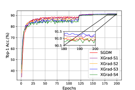
(a) AlexNet

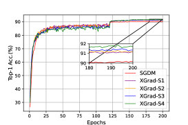
(b) VGG-11

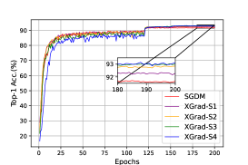
(c) VGG-16

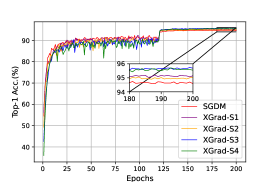
(d) ResNet-34

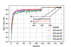
(e) ResNet-101

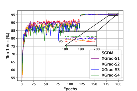
(f) GoogleNet

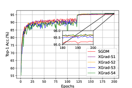
(g) DenseNet-121

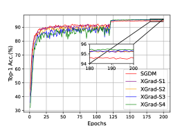
(h) Inception-V3

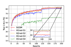
(i) ViT

Figure 2: Validation Top-1 accuracy vs. epochs of training CNNs on CIFAR-10.

TABLE IV: Comparisons of XGrad and SGDM when training on CIFAR-10. The best results are highlighted in bold face.

Optimizers	AlexNet	VGG-11	VGG-16	ResNet-34	ResNet-101	GoogleNet	DenseNet-121	Inception-V3	ViT
Maximum Top-1 Accuracy
SGDM	91.00%	90.09%	91.76%	94.74%	95.08%	95.07%	95.25%	94.64%	82.30%
XGrad-S1	91.32%	91.23%	92.36%	95.21%	95.42%	95.43%	95.72%	95.36%	83.71%
XGrad-S2	91.09%	91.34%	92.87%	95.06%	95.44%	95.23%	95.73%	95.39%	83.90%
XGrad-S3	91.42%	91.50%	93.04%	95.74%	95.65%	95.37%	95.62%	95.40%	81.77%
XGrad-S4	91.01%	91.90%	93.19%	95.71%	95.63%	95.60%	95.77%	95.56%	61.96%
Maximum Top-5 Accuracy
SGDM	91.00%	99.69%	99.59%	99.81%	99.86%	99.90%	99.87%	99.83%	99.23%
XGrad-S1	99.78%	99.58%	99.58%	99.88%	99.92%	99.87%	99.90%	99.90%	99.46%
XGrad-S2	99.72%	99.60%	99.65%	99.88%	99.89%	99.87%	99.93%	99.90%	99.42%
XGrad-S3	99.75%	99.64%	99.63%	99.90%	99.90%	99.90%	99.94%	99.90%	99.19%
XGrad-S4	99.72%	99.72%	99.74%	99.93%	99.93%	99.94%	99.95%	99.91%	96.74%
Minimum Loss
SGDM	0.358	0.437	0.390	0.231	0.213	0.187	0.198	0.237	0.532
XGrad-S1	0.328	0.382	9.351	0.206	0.183	0.170	0.175	0.189	0.482
XGrad-S2	0.334	0.356	0.305	0.194	0.183	0.167	0.165	0.177	0.494
XGrad-S3	0.326	0.331	0.292	0.171	0.166	0.161	0.162	0.178	0.543
XGrad-S4	0.332	0.323	0.278	0.173	0.166	0.153	0.156	0.172	1.056

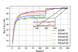
(a) AlexNet

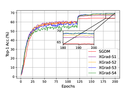
(b) VGG-11

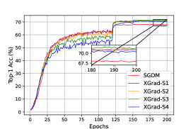
(c) VGG-16

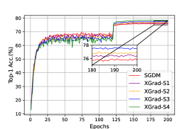
(d) ResNet-34

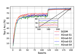
(e) ResNet-101

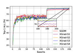
(f) GoogleNet

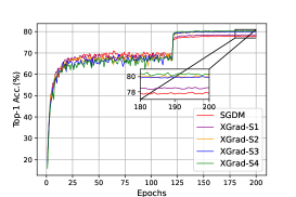
(g) DenseNet-121

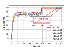
(h) Inception-V3

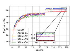
(i) ViT

Figure 3: Validation Top-1 accuracy vs. epochs of training CNNs on CIFAR-100.

TABLE V: Comparisons of XGrad and SGDM when training on CIFAR-100. The best results are highlighted in bold face.

Optimizers	AlexNet	VGG-11	VGG-16	ResNet-34	ResNet-101	GoogleNet	DenseNet-121	Inception-V3	ViT
Maximum Top-1 Accuracy
SGDM	69.48%	64.42%	68.17%	75.99%	77.02%	77.43%	77.96%	77.60%	58.23%
XGrad-S1	70.34%	67.33%	71.01%	76.57%	77.76%	78.17%	78.60%	79.25%	61.27%
XGrad-S2	70.31%	68.18%	71.19%	77.05%	78.34%	79.40%	80.19%	78.37%	62.51%
XGrad-S3	70.21%	69.06%	71.57%	77.66%	79.31%	79.26%	80.05%	79.09%	63.12%
XGrad-S4	69.48%	69.26%	70.83%	78.62%	78.47%	79.61%	80.55%	80.39%	63.77%
Maximum Top-5 Accuracy
SGDM	91.32%	85.06%	86.44%	93.31%	93.69%	94.13%	94.01%	94.09%	82.51%
XGrad-S1	91.88%	87.10%	88.46%	93.56%	94.34%	94.31%	94.46%	94.90%	85.70%
XGrad-S2	92.03%	87.92%	89.89%	93.99%	94.58%	95.11%	95.00%	94.61%	87.36%
XGrad-S3	91.50%	88.48%	90.19%	94.05%	94.98%	95.12%	95.32%	94.93%	88.03%
XGrad-S4	91.21%	88.41%	89.77%	94.36%	94.83%	95.27%	95.87%	95.33%	88.49%
Minimum Loss
SGDM	1.245	1.740	1.652	1.038	0.990	0.924	1.020	1.000	1.842
XGrad-S1	1.183	1.653	1.389	0.958	0.925	0.881	0.940	0.854	1.616
XGrad-S2	1.162	1.494	1.260	0.915	0.900	0.805	0.843	0.858	1.442
XGrad-S3	1.158	1.373	1.290	0.906	0.850	0.806	0.812	0.809	1.364
XGrad-S4	1.179	1.347	1.241	0.871	0.852	0.789	0.766	0.771	1.371

Figure 2 presents the learning curves for training CNN and ViT models on the CIFAR-10 dataset. Table IV summarizes the obtained maximum validation top-1/5 accuracy and minimum validation loss. Figure 3 shows the learning curves for training CNN models on the CIFAR-100 dataset. Table V summarizes the obtained maximum top-1/5 validation accuracy and the minimum validation loss. In all figures of Figures 2 and 3, we let the red lines illustrate the learning curves of SGDM and let other colored lines represent the learning curves of XGrad.

Based on the observation of Table IV and Figure 2, we can immediately reach the following conclusions. First, the learning curves of XGrad with different weight prediction steps tend to be lower than that of SGDM at the beginning training period. Yet, as the decaying of the learning rate, XGrad gradually surpasses SGDM and always gets higher top-1 accuracy than SGDM at the end of the training period. This demonstrates that XGrad tends to be inferior to SGDM with a large learning rate but outperforms SGDM with a small learning rate. Second, Table IV illustrates that XGrad outperforms SGDM on all evaluated DNN models in terms of the obtained validation accuracy and loss. In particular, XGrad achieves consistently higher top-1/5 validation accuracy and lower validation loss than SGDM. Compared to SGDM, XGrad respectively achieves an improvement of 0.42%, 1.81%, 1.43%, 1.00%, 0.57%, 0.53%, 0.52%, 0.92%, and 0.79% top-1 accuracy for training AlexNet, VGG-11, VGG-16, ResNet-34, ResNet-101, GoogleNet, DenseNet-121, Inception-V3, and ViT. On average, our proposal yields 0.89% (up to 1.81%) top-1 accuracy improvement over SGDM. Third, comparing the experimental results of XGrad-S1, XGrad-S2, XGrad-S3, and XGrad-S4, we can see that XGrad with different weight prediction steps consistently gets good results for all CNN models. The special case is training ViT on CIFAR10, where XGrad-S4 performs poorly and obtains the minimum validation accuracy.

We can draw similar conclusions from the observation of the experiment results shown in Table V and Figure 3. First, the learning curves of SGDM seem to be higher than that of XGrad at the beginning of the training but to be lower than that of XGrad at the end of the training. This again validates the effect of learning rate on the performance of XGrad. Second, Table V illustrates that XGrad achieves consistently higher validation accuracy and lower validation loss than SGDM. Specially, XGrad yields 0.86%, 4.84%, 3.40%, 1.67%, 2.63%, 2.29%, 2.23%, 2.79%, and 5.54% more top-1 accuracy than SGDM when training AlexNet, VGG-11, VGG-16, ResNet-34, ResNet-101, GoogleNet, DenseNet-121 and Inception-V3, respectively. That is to say, XGrad can achieve an average of 2.92% (up to 5.54%) top-1 accuracy improvement over SGDM. Third, when comparing the experimental results of XGrad-S1, XGrad-S2, XGrad-S3, and XGrad-S4, we can see that XGrad always achieves comparable high performance.

V-B2 Comparisons of XGrad with Adam

In this section, we selected LeNet, ResNet-34, DenseNet-121, Inception-V3, ViT, LSTM-1, LSTM-2, and GNMT-8 as the benchmark models. Concretely, we trained LeNet on FashionMNIST on Fashion-MNIST for 50 epochs with a fixed learning rate of $1e^{-3}$ and a mini-batch size of 128. We trained ResNet-34, DenseNet-121, Inception-V3, and ViT on CIFAR-10 for 120 epochs with a mini-batch size of 128. The initial learning rate was $1e^{-3}$ and was divided by 10 at the 90th epoch. We trained LSTM-1 and LSTM-2 on the Penn TreeBank Dataset [38] for 200 epochs with a mini-batch size of 20. The initial learning rate was $1e^{-3}$ and was decayed by 0.1 at the 100th and 145th epoch. We trained GNMT-8 on WMT-16 En$\rightarrow$De for 6 epochs with a steady learning rate of $3e^{-4}$ and a mini-batch size of 128. For both XGrad and Adam, we always evaluated them with the default parameters, i.e., $\beta_{1}$=0.9, $\beta_{2}$=0.999, and $\epsilon=10^{-8}$. The weight decay for both approaches was set to $\lambda=5e^{-4}$.

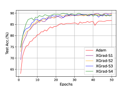
(a) LeNet

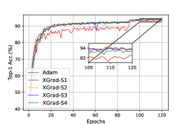
(b) ResNet-34

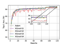
(c) DenseNet-121

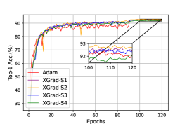
(d) Inception-V3

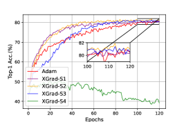
(e) ViT

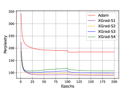
(f) LSTM-1

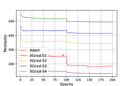
(g) LSTM-2

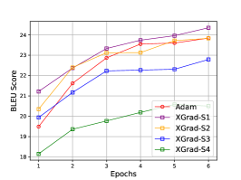
(h) GNMT-8

Figure 4: Comparision of Adam and XGrad when training CNNs.

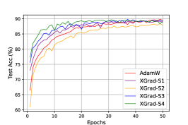
(a) LeNet

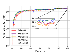
(b) ResNet-34

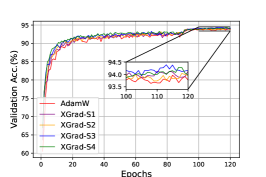
(c) DenseNet-121

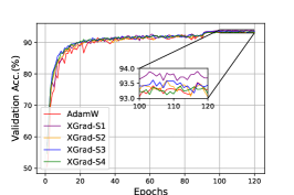
(d) Inception-V3

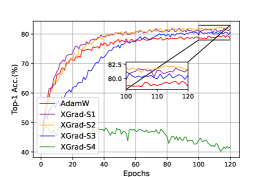
(e) ViT

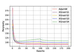
(f) LSTM-1

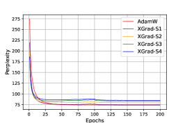
(g) LSTM-2

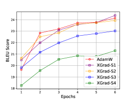
(h) GNMT-8

Figure 5: Comparision of AdamW and XGrad when training CNNs on CIFAR-10.

TABLE VI: Comparisons of Adam and XGrad. The best results are highlighted in bold face.

Optimizers	LeNet	ResNet-34	DenseNet-121	Inception-V3	ViT	LSTM-1	LSTM-2	GNMT-8
Best Accuracy
Adam	86.85%	93.30%	92.75%	92.47%	80.91%	183.23	178.02	23.84
XGrad-S1	89.95%	94.07%	93.75%	92.69%	80.80%	89.19	132.41	24.35
XGrad-S2	89.57%	94.15%	93.48%	92.94%	81.89%	92.39	343.09	23.83
XGrad-S3	89.51%	94.09%	93.60%	92.56%	81.41%	98.21	414.54	22.79
XGrad-S4	89.94%	93.85%	93.72%	92.11%	50.53%	106.25	495.09	20.50

TABLE VII: Comparisons of AdamW and XGrad. The best results are highlighted in bold face.

Optimizers	LeNet	ResNet-34	DenseNet-121	Inception-V3	ViT	LSTM-1	LSTM-2	GNMT-8
Best Accuracy
AdamW	89.83%	94.03%	93.97%	93.53%	79.48%	88.45	73.87	24.14
XGrad-S1	89.36%	94.06%	94.13%	93.90%	81.88%	89.10	74.65	24.37
XGrad-S2	89.43%	93.95%	94.04%	93.60%	82.28%	92.27	79.25	23.93
XGrad-S3	89.83%	94.37%	94.39%	93.61%	80.96%	98.20	82.97	23.02
XGrad-S4	89.68%	94.44%	94.29%	93.41%	49.71%	106.39	85.17	21.30

Figures 4(a),  4(b),  4(c),  2(h), and 4(e) show the curves about accuracy (higher is better) vs. epochs. Figures 4(f) and 4(g) illustrates the curves about perplexity (lower is better) vs. epochs. Figure 4(h) illustrate the curves about BLEU score (higher is better) vs. epochs. Table VI summarizes the best model accuracy. For LeNet, ResNet-34, DenseNet-121, and Inception-V3, the model accuracy means maximum top-1 accuracy. For LSTM-1 and LSTM-2 the model accuracy means the minimum perplexity (lower is better); For GNMT-8, the model accuracy means the maximum BLEU score (higher is better).

Figure 4(a) shows that XGrad with different weight prediction steps always attains higher accuracy than Adam when training with the same epochs. Figures 4(b),  4(c) and 4(f) also demonstrate that XGrad with different weight prediction steps always outperforms Adam in terms of convergence trait. While Figures 4(d),  4(e),  4(g), and 4(h) reveals slightly different results. The convergence of XGrad tends to be worse as the increase of weight prediction step. In particular, the convergence of XGrad with weight prediction step size 4 (i.e., XGrad-S4) is always inferior to Adam when training Inception-V3, ViT, LSTM-2, and GNMT-8.

The experiment results shown in Table VI again validates the effectiveness of XGrad. Compared to Adam, XGrad achieves an accuracy improvement of 3.10%, 0.85%, 1.00%, 0.47%, and 0.98% when training LeNet, ResNet-34, DenseNet-121, Inception-V3, and ViT. This means that XGrad leads to an average of 1.28% accuracy improvement over Adam. Meanwhile, XGrad achieves 94.04 and 45.61 less perplexity than Adam when training LSTM-1 and LSTM-2, respectively. XGrad also obtains a 0.49 more BLEU score than Adam when training GNMT-8. When comparing XGrad-S1, XGrad-S2, XGrad-S3, and XGrad-S4, we can also see that XGrad with smaller $s$ ($s\leq 2$) tends to achieve the best model accuracy.

V-B3 Comparisons of XGrad with AdamW

In this section, we again selected LeNet, ResNet-34, DenseNet-121, Inception-V3, ViT, LSTM-1, LSTM-2, and GNMT-8 as the benchmark models and evaluated them with the same experimental settings as described in Section V-B2. Figures 5(a),  5(b),  5(c),  2(h), and 5(e) show the curves about test/validation accuracy (higher is better) vs. epochs. Figures 5(f) and 5(g) illustrate the curves about perplexity (lower is better) vs. epochs. Figure 5(h) illustrates the curves about BLEU score (higher is better) vs. epochs. Table VII summarizes the best model accuracy. Likewise, the best model accuracy of LeNet, ResNet-34, DenseNet-121, and Inception-V3 refers to maximum top-1 accuracy; the best model accuracy of LSTM-1 and LSTM-2 denotes the minimum perplexity; the best model accuracy of GNMT-8 means the maximum BLEU score.

We can reach the following conclusions based on the observation of the experiment results. First, XGrad performs better than AdamW on the image classification and machine translation tasks. On average, XGrad yields 1.0% (up to 2.8%) top-1 accuracy improvement over AdamW. XGrad also achieves a higher BLEU score (24.35 versus 23.84) when training GNMT-8. Second, XGrad performs slightly worse than AdamW on the language modeling tasks. AdamW gets 0.65 and 0.78 less perplexity than XGrad when training LSTM-1 and LSTM-2, respectively. Third, for the image classification task, the weight prediction step has little effect on the model accuracy generated by the XGrad. However, for language modeling and machine translation tasks, the performance of XGrad tends to be worse with the increase in weight prediction steps.

TABLE VIII: 1-epoch running time (in seconds) comparison of XGrad vs. SGDM.

Optimizers	VGG-16	ResNet-34	ResNet-101	GoogleNet	DenseNet-121	Inception-V3	ViT
SGDM	12.59s	36.20s	131.73s	94.81s	82.41s	191.81s	40.34s
XGrad	13.29s	38.25s	139.09s	99.43s	92.70s	196.42s	41.60s

TABLE IX: 1-epoch running time (in seconds/minutes) comparison of XGrad vs. Adam.

Optimizers	ResNet-34	DenseNet-121	Inception-V3	ViT	LSTM-1	LSTM-2	GNMT-8
Adam	37.01s	95.34s	200.63s	40.72s	21.03s	25.38s	386m
XGrad	44.36s	115.99s	207.78s	43.54s	24.96s	26.43s	400m

(a) XGrad vs. SGDM

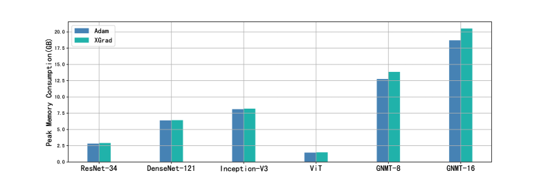
(b) XGrad vs. Adam

Figure 6: Comparisons of Peak GPU memory consumption (in GB).

V-C Computational cost

In this section, we evaluate the computational cost of XGrad. We mainly compare XGrad with SGDM and Adam. For the comparison of XGrad and SGDM, we select VGG-16, ResNet-34, ResNet-101, GoogleNet, DenseNet-121, Inception-V3, and ViT as the benchmark models. For the comparison of XGrad and Adam, we select ResNet-34, DenseNet-121, Inception-V3, ViT, LSTM-1, LSTM-2, and GNMT-8 as the benchmark models. For the comparison of XGrad and SGDM, we trained all the DNN models on CIFAR-10 with the same experimental settings described in Section V-B1. For the comparison of XGrad and Adam, we evaluated all the DNN models with the same experimental settings described in Section V-B2. Table VIII reports the running time of 1-epoch training when comparing XGrad with SGDM. While Table IX summarizes the experimental results of the comparison of XGrad and Adam.

The experimental results shown in both Tables VIII and IX demonstrate that XGrad always incurs longer training time than the original gradient-based optimizer. XGrad incurs an average of 5.67% (up to 12.48%) longer training time than SGDM. In comparison with Adam, XGrad leads to 11.21% longer training time on average. The experimental results are understandable as the weight prediction increased additional computations compared to the original gradient-based optimizers. Nevertheless, we see that the increased computations are quite limited and sometimes can even be neglected.

V-D Memory consumption

In this section, we evaluate the memory consumption of XGrad. We mainly compare the peak GPU memory consumption of XGrad with that of SGDM and Adam incorporated in PyTorch. Likewise, the comparisons are divided into two groups: XGrad vs. SGDM and XGrad vs. Adam. For the comparison of XGrad vs. SGDM, we evaluated seven CNN models on CIFAR10 including VGG-16, ResNet-34, ResNet-101, GoogleNet, DenseNet-121, Inception-V3, and ViT. For the comparisons of XGrad vs. Adam, the evaluated DNN models include ResNet-34, DenseNet-121, Inception-V3, ViT, LSTM-2, and GNMT-8. The experimental settings are the same as in Section V-C.

Figure 6 illustrates the peak GPU memory consumption of XGrad and other popular optimizers including SGDM and Adam From the observation of Figure 6(a), we can immediately reach the following conclusions. First, for any evaluated model, XGrad always consumes almost the same (only slightly more) GPU memory as SGDM. On average, XGrad only incurs 1.8% (up to 3.0%) more GPU memory than SGDM. We can draw similar conclusions from the experimental results shown in Figure 6(b). XGrad leads to an average of 5.0% (up to 9.7%) more GPU memory consumption than Adam.

Overall, the experimental results shown in Figure 6 reveal that XGrad incurs slightly more GPU memory consumption than the original gradient-based optimizers incorporated in the torch.optim package. This is reasonable because XGrad requires storing more intermediate variables in GPU memory to achieve weight prediction. However, we note that the increased GPU memory consumption is quite limited.

VI Concluding remarks

To further boost the convergence and generation of popular gradient-based optimizers, in this paper, we introduce weight prediction into the DNN training and propose a new DNN training framework called XGrad. Our proposal can improve the convergence and generalization of popular gradient-based optimizers with a cost of slightly increasing the training time and GPU memory consumption. The remarkable feature of our proposal is that we perform both forward pass and backward propagation using the future weights which are predicted according to the specific update rule of the used optimizer. In particular, we construct the mathematical relationship between currently available weights and future weights and devise an effective way to incorporate weight prediction into DNN training. The proposed framework covers many of the most frequently used gradient-based optimizers such as SGD with momentum, AdaGrad, RMSProp, Adam, and AdamW.

XGrad is easy to implement and works well in boosting the convergence of DNN training. Extensive experimental results on image classification, language modeling, and machine translation tasks verify the effectiveness of our proposal. We believe that other adaptive gradient methods such as AdaBelief, AdaBound, RAdam, Yogi, etc can be easily incorporated into our proposed framework.

For future work, we would like to explore the internal mechanism of weight prediction from a mathematical perspective. Furthermore, we will study the relationship between the weight prediction steps and the learning rate, as well as their impacts on the convergence and generalization of DNN training.

References

- [1] N. Qian, “On the momentum term in gradient descent learning algorithms,” Neural networks, vol. 12, no. 1, pp. 145–151, 1999.
- [2] I. Sutskever, J. Martens, G. Dahl, and G. Hinton, “On the importance of initialization and momentum in deep learning,” in International conference on machine learning. PMLR, 2013, pp. 1139–1147.
- [3] D. P. Kingma and J. Ba, “Adam: A method for stochastic optimization,” arXiv preprint arXiv:1412.6980, 2014.
- [4] I. Loshchilov and F. Hutter, “Decoupled weight decay regularization,” arXiv preprint arXiv:1711.05101, 2017.
- [5] K. Simonyan and A. Zisserman, “Very deep convolutional networks for large-scale image recognition,” arXiv preprint arXiv:1409.1556, 2014.
- [6] C. Szegedy, W. Liu, Y. Jia, P. Sermanet, S. Reed, D. Anguelov, D. Erhan, V. Vanhoucke, and A. Rabinovich, “Going deeper with convolutions,” in Proceedings of the IEEE conference on computer vision and pattern recognition, 2015, pp. 1–9.
- [7] K. He, X. Zhang, S. Ren, and J. Sun, “Deep residual learning for image recognition,” in Proceedings of the IEEE conference on computer vision and pattern recognition, 2016, pp. 770–778.
- [8] A. Krizhevsky, I. Sutskever, and G. E. Hinton, “Imagenet classification with deep convolutional neural networks,” Communications of the ACM, vol. 60, no. 6, pp. 84–90, 2017.
- [9] Z. Li, K. Meidani, P. Yadav, and A. Barati Farimani, “Graph neural networks accelerated molecular dynamics,” The Journal of Chemical Physics, vol. 156, no. 14, p. 144103, 2022.
- [10] C. Chen, W. Ye, Y. Zuo, C. Zheng, and S. P. Ong, “Graph networks as a universal machine learning framework for molecules and crystals,” Chemistry of Materials, vol. 31, no. 9, pp. 3564–3572, 2019.
- [11] K. Choudhary and B. DeCost, “Atomistic line graph neural network for improved materials property predictions,” npj Computational Materials, vol. 7, no. 1, p. 185, 2021.
- [12] I. Goodfellow, J. Pouget-Abadie, M. Mirza, B. Xu, D. Warde-Farley, S. Ozair, A. Courville, and Y. Bengio, “Generative adversarial networks,” Communications of the ACM, vol. 63, no. 11, pp. 139–144, 2020.
- [13] A. Vaswani, N. Shazeer, N. Parmar, J. Uszkoreit, L. Jones, A. N. Gomez, Ł. Kaiser, and I. Polosukhin, “Attention is all you need,” Advances in neural information processing systems, vol. 30, 2017.
- [14] J. Devlin, M.-W. Chang, K. Lee, and K. Toutanova, “Bert: Pre-training of deep bidirectional transformers for language understanding,” arXiv preprint arXiv:1810.04805, 2018.
- [15] A. Dosovitskiy, L. Beyer, A. Kolesnikov, D. Weissenborn, X. Zhai, T. Unterthiner, M. Dehghani, M. Minderer, G. Heigold, S. Gelly et al., “An image is worth 16x16 words: Transformers for image recognition at scale,” arXiv preprint arXiv:2010.11929, 2020.
- [16] K. Han, Y. Wang, H. Chen, X. Chen, J. Guo, Z. Liu, Y. Tang, A. Xiao, C. Xu, Y. Xu et al., “A survey on vision transformer,” IEEE transactions on pattern analysis and machine intelligence, vol. 45, no. 1, pp. 87–110, 2022.
- [17] A. Radford, J. Wu, R. Child, D. Luan, D. Amodei, I. Sutskever et al., “Language models are unsupervised multitask learners,” OpenAI blog, vol. 1, no. 8, p. 9, 2019.
- [18] T. Brown, B. Mann, N. Ryder, M. Subbiah, J. D. Kaplan, P. Dhariwal, A. Neelakantan, P. Shyam, G. Sastry, A. Askell et al., “Language models are few-shot learners,” Advances in neural information processing systems, vol. 33, pp. 1877–1901, 2020.
- [19] L. Bottou, F. E. Curtis, and J. Nocedal, “Optimization methods for large-scale machine learning,” SIAM review, vol. 60, no. 2, pp. 223–311, 2018.
- [20] L. Guan, W. Yin, D. Li, and X. Lu, “Xpipe: Efficient pipeline model parallelism for multi-gpu dnn training,” arXiv preprint arXiv:1911.04610, 2019.
- [21] C.-C. Chen, C.-L. Yang, and H.-Y. Cheng, “Efficient and robust parallel dnn training through model parallelism on multi-gpu platform,” arXiv preprint arXiv:1809.02839, 2018.
- [22] J. Duchi, E. Hazan, and Y. Singer, “Adaptive subgradient methods for online learning and stochastic optimization.” Journal of machine learning research, vol. 12, no. 7, 2011.
- [23] T. Tieleman and G. Hinton, “Lecture 6.5-rmsprop, coursera: Neural networks for machine learning,” University of Toronto, Technical Report, vol. 6, 2012.
- [24] L. Guan, “Weight prediction boosts the convergence of adamw,” arXiv preprint arXiv:2302.00195, 2023.
- [25] G. E. Hinton, S. Osindero, and Y.-W. Teh, “A fast learning algorithm for deep belief nets,” Neural computation, vol. 18, no. 7, pp. 1527–1554, 2006.
- [26] M. D. Zeiler, “Adadelta: an adaptive learning rate method,” arXiv preprint arXiv:1212.5701, 2012.
- [27] J. Zhuang, T. Tang, Y. Ding, S. C. Tatikonda, N. Dvornek, X. Papademetris, and J. Duncan, “Adabelief optimizer: Adapting stepsizes by the belief in observed gradients,” Advances in neural information processing systems, vol. 33, pp. 18 795–18 806, 2020.
- [28] M. Zaheer, S. Reddi, D. Sachan, S. Kale, and S. Kumar, “Adaptive methods for nonconvex optimization,” Advances in neural information processing systems, vol. 31, 2018.
- [29] L. Luo, Y. Xiong, Y. Liu, and X. Sun, “Adaptive gradient methods with dynamic bound of learning rate,” arXiv preprint arXiv:1902.09843, 2019.
- [30] L. Liu, H. Jiang, P. He, W. Chen, X. Liu, J. Gao, and J. Han, “On the variance of the adaptive learning rate and beyond,” arXiv preprint arXiv:1908.03265, 2019.
- [31] Y. Wang, Y. Kang, C. Qin, H. Wang, Y. Xu, Y. Zhang, and Y. Fu, “Rethinking adam: A twofold exponential moving average approach,” arXiv preprint arXiv:2106.11514, 2021.
- [32] S. J. Reddi, S. Kale, and S. Kumar, “On the convergence of adam and beyond,” in International Conference on Learning Representations.
- [33] Y. E. Nesterov, “A method of solving a convex programming problem with convergence rate obigl(k^2bigr),” in Doklady Akademii Nauk, vol. 269, no. 3. Russian Academy of Sciences, 1983, pp. 543–547.
- [34] T. Dozat, “Incorporating nesterov momentum into adam,” 2016.
- [35] X. Chen, S. Liu, R. Sun, and M. Hong, “On the convergence of a class of adam-type algorithms for non-convex optimization,” arXiv preprint arXiv:1808.02941, 2018.
- [36] H. Xiao, K. Rasul, and R. Vollgraf, “Fashion-mnist: a novel image dataset for benchmarking machine learning algorithms,” arXiv preprint arXiv:1708.07747, 2017.
- [37] A. Krizhevsky, G. Hinton et al., “Learning multiple layers of features from tiny images,” 2009.
- [38] M. A. Marcinkiewicz, “Building a large annotated corpus of english: The penn treebank,” Using Large Corpora, vol. 273, 1994.
- [39] R. Sennrich, B. Haddow, and A. Birch, “Edinburgh neural machine translation systems for wmt 16,” arXiv preprint arXiv:1606.02891, 2016.
- [40] Y. LeCun, L. Bottou, Y. Bengio, and P. Haffner, “Gradient-based learning applied to document recognition,” Proceedings of the IEEE, vol. 86, no. 11, pp. 2278–2324, 1998.
- [41] G. Huang, Z. Liu, L. Van Der Maaten, and K. Q. Weinberger, “Densely connected convolutional networks,” in Proceedings of the IEEE conference on computer vision and pattern recognition, 2017, pp. 4700–4708.
- [42] C. Szegedy, V. Vanhoucke, S. Ioffe, J. Shlens, and Z. Wojna, “Rethinking the inception architecture for computer vision,” in Proceedings of the IEEE conference on computer vision and pattern recognition, 2016, pp. 2818–2826.
- [43] Y. Wu, M. Schuster, Z. Chen, Q. V. Le, M. Norouzi, W. Macherey, M. Krikun, Y. Cao, Q. Gao, K. Macherey et al., “Google’s neural machine translation system: Bridging the gap between human and machine translation,” arXiv preprint arXiv:1609.08144, 2016.