Background Filter: A method for removing signal contamination during significance estimation of a GstLAL anaysis

Abstract

To evaluate the probability of a gravitational-wave candidate originating from noise, GstLAL collects noise statistics from the data it analyzes. Gravitational-wave signals of astrophysical origin get added to the noise statistics, harming the sensitivity of the search. We present the Background Filter, a novel tool to prevent this by removing noise statistics that were collected from gravitational-wave candidates. To demonstrate its efficacy, we analyze one week of LIGO and Virgo O3 data, and show that it improves the sensitivity of the analysis by 20-40% in the high mass region, in the presence of 868 simulated gravitational-wave signals. With the upcoming fourth observing run of LIGO, Virgo, and KAGRA expected to yield a high rate of gravitational-wave detections, we expect the Background Filter to be an important tool for increasing the sensitivity of a GstLAL analysis.

I Introduction

The Laser Interferometer Gravitational-wave Observatory (LIGO) Aasi et al. (2015) and Virgo Acernese et al. (2015) collaborations have revolutionized the field of gravitational-wave (GW) astronomy by detecting black hole and neutron star mergers Abbott et al. (2019); gwt (2021); The LIGO Scientific Collaboration et al. (2021); Abbott et al. (2021a). The detections have allowed us to observe the universe in new ways and have opened up new avenues of scientific inquiry. Abbott et al. (2021b, c); the LIGO Scientific Collaboration et al. (2023); Magee et al. (2018) The GstLAL GW search pipeline Messick et al. (2017); Sachdev et al. (2019); Hanna et al. (2020); Cannon et al. (2021) (referred to as GstLAL hereafter) has been a significant contributor to this field. In particular, GstLAL’s ability to detect signals in low-latency 170817_gcn (170) has facilitated multi-messenger observations Abbott et al. (2017).

GstLAL is a GW search pipeline that can process data from ground-based GW detectors, such as the Hanford and Livingston LIGO detectors, the Virgo detector and the KAGRA detector Akutsu et al. (2020), in near real time. It makes use of time-domain matched-filtering to enable the detection of signals in noise-dominated data. It uses a likelihood ratio (LR) Tsukada et al. (2023); Cannon et al. (2015, 2013) as a ranking statistic for assigning significance to detections. GstLAL divides its template bank Mukherjee et al. (2018); Sakon et al. (2022) into different “template bins” to reduce the computational cost of the analysis, and analyzes each one separately. Some of these techniques are also used by other search pipelines, such as PyCBC Canton et al. (2021); Davies et al. (2020); Nitz (2018), MBTA Aubin et al. (2021); Adams et al. (2016), SPIIR Chu (2022, 2017), and IAS Venumadhav et al. (2019); Zackay et al. (2021).

The fourth observing run of the LIGO Scientific, Virgo and KAGRA collaboration (O4) is set to begin in May 2023 o4d and promises to provide improved detector sensitivity. GstLAL will continue to play an essential role in the detection of new GW candidates. As such, it is necessary to keep refining the analysis pipeline to reap the benefits of improved detector sensitivity to detect even more, and new types of candidates. The Background Filter is one such new feature to this end.

This paper is structured as follows. In Sec. II, we introduce the LR used by GstLAL, in particular the $\rho-\xi^{2}$ histograms that GstLAL uses to evaluate one term of the likelihood ratio, and how the presence of GW signals in the data can cause “contamination” of these histograms. In Sec. III, we describe how the Background Filter works, and how it removes this contamination. Finally, in Sec. IV, we describe the analyses we performed to evaluate the performance of the Background Filter, and the impact it has on the sensitivity of a GstLAL analysis.

II Signal Contamination

II.1 Likelihood Ratio

GstLAL is a matched-filtering based GW search pipeline which uses a likelihood ratio statistic to rank GW candidates  Tsukada et al. (2023); Cannon et al. (2015). The LR is defined as

$$\mathcal{L}=\frac{P\left(\vec{O},\vec{\rho},\vec{\xi^{2}},\vec{t},\vec{\phi},\bar{\theta}\mid\mathcal{H}_{\mathrm{s}}\right)}{P\left(\vec{O},\vec{\rho},\vec{\xi^{2}},\vec{t},\vec{\phi},\bar{\theta}\mid\mathcal{H}_{\mathrm{n}}\right)},$$ (1)

where the numerator is the probability of obtaining a GW candidate with parameters $(\vec{O},\vec{\rho},\vec{\xi^{2}},\vec{t},\vec{\phi},\bar{\theta})$, under the signal hypothesis ($\mathcal{H}_{\mathrm{s}}$) and the denominator is the probability of obtaining the same candidate under the noise hypothesis ($\mathcal{H}_{\mathrm{n}}$). $\vec{O}$ is the subset of GW detectors that the candidate was found in, $\vec{\rho}$ is the set of matched-filtering signal-to-noise-ratios (SNRs) of those detectors, $\vec{\xi^{2}}$ is the set of $\xi^{2}$-signal-based-veto values, $\vec{t},\vec{\phi}$ are the times and phases with which the candidate was found in the detectors, and $\bar{\theta}$ is the template which recovered the candidate, which also represents a set of intrinsic parameters (masses and spins).

The LR can be factorized as

$$\mathcal{L}=\frac{P\left(\bar{\theta}\mid\mathcal{H}_{\mathrm{s}}\right)\times P\left(t_{\mathrm{ref}},\phi_{\mathrm{ref}}\mid\bar{\theta},\mathcal{H}_{\mathrm{s}}\right)\times P\left(\vec{O}\mid t_{\mathrm{ref}},\mathcal{H}_{\mathrm{s}}\right)\times P\left(\vec{\rho},\vec{\Delta t},\vec{\Delta\phi}\mid\vec{O},t_{\mathrm{ref}},\mathcal{H}_{\mathrm{s}}\right)\times P\left(\vec{\xi^{2}}\mid\vec{\rho},\bar{\theta},\mathcal{H}_{\mathrm{s}}\right)}{P\left(t_{\mathrm{ref}},\bar{\theta}\mid\mathcal{H}_{\mathrm{n}}\right)\times P\left(\vec{O}\mid t_{\mathrm{ref}},\bar{\theta},\mathcal{H}_{\mathrm{n}}\right)\times P\left(\vec{\Delta t},\vec{\phi}\mid\vec{O},\mathcal{H}_{\mathrm{n}}\right)\times P\left(\vec{\rho},\vec{\xi^{2}}\mid t_{\mathrm{ref}},\bar{\theta},\mathcal{H}_{\mathrm{n}}\right)}$$ (2)

For a comprehensive explanation of Eq. (2) and every individual term in the LR, readers are referred to Tsukada et al. (2023). For the purpose of this paper, we are only concerned with the last term in the denominator, $P\left(\vec{\rho},\vec{\xi^{2}}\mid t_{\mathrm{ref}},\bar{\theta},\mathcal{H}_{\mathrm{n}}\right)$ (hereby referred to as the $\rho-\xi^{2}$ noise LR term).

II.2 The $\rho-\xi^{2}$ histograms

The $\rho-\xi^{2}$ noise LR term is calculated in a data-driven way. GstLAL creates a histogram for each detector and template bin in $\rho-\xi^{2}$ space, called $\rho-\xi^{2}$ background histograms, and populates it with the ($\rho$, $\xi^{2}$) values of noise events found in that template bin during the analysis. Then, the $\rho-\xi^{2}$ noise LR term can be calculated by evaluating the probability density function represented by the histograms at the relevant ($\vec{\rho}$, $\vec{\xi^{2}}$) value.

Since the $\rho-\xi^{2}$ noise LR term assumes the noise hypothesis, we need to populate the histograms with events originating only from noise, as compared to events originating from GW candidates. To a large degree, this is achieved by requiring those events to be recovered only in one detector (called a single-detector or single event in contrast to a coincident event) during a time when more than one detector was producing data (called coincident time in contrast to single time). This is because we expect GW signals to be correlated across detectors, but not noise events.

Despite this, GW signals can sometimes enter the $\rho-\xi^{2}$ histograms. The reason might be astrophysical in origin, e.g. the GW source is located in the blind spot of all but one detector, or it might be terrestrial, e.g. only one detector is sensitive enough to pick up the GW signal. In addition, GW signals which are recovered as coincident events in one template bin sometimes also get recovered as a single event, with a lower $\rho$ and LR in other neighbouring template bins, which don’t contain templates with high $\rho$ for that GW signal. We say a bin has a good match with a GW signal if it has templates with a high $\rho$ for that GW signal, and that it has a bad match otherwise. GW events being recovered as coincident events in one bin and as single events in others is demonstrated in Fig. 1 for GW200129_065458, a known GW candidate reported in GWTC-3 Abbott et al. (2021a). The candidate is recovered as a coincident event in bin 818, with which it has the best match. It is also recovered in bin 838 as a Livingston single with a lower $\rho$, since it’s match with that bin isn’t as good. As a result, the candidate will be added to the background histogram of bin 838. Gravitational wave signals entering the background histograms is commonly called signal contamination of the $\rho-\xi^{2}$ background histograms. The contamination caused by GW200129_065458 in the background histogram of bin 838 is shown in Fig. 3. Since the GW signal gets added to the background histogram, it occupies a region in $\rho-\xi^{2}$ space typical of signals, but not of noise. As a result, we see a protrusion to the histogram, which is generally how signal contamination manifests visually.

Signal contamination can result in the $\rho-\xi^{2}$ histograms not accurately reflecting the noise characteristics of the data, and as a result, the $\rho-\xi^{2}$ noise LR term will not be calculated correctly. In general, it can cause the $\rho-\xi^{2}$ noise LR term for GW candidates to be evaluated higher than it’s true value, leading to lower LR values of candidates. In short, signal contamination can lower the sensitivity of the GW search.

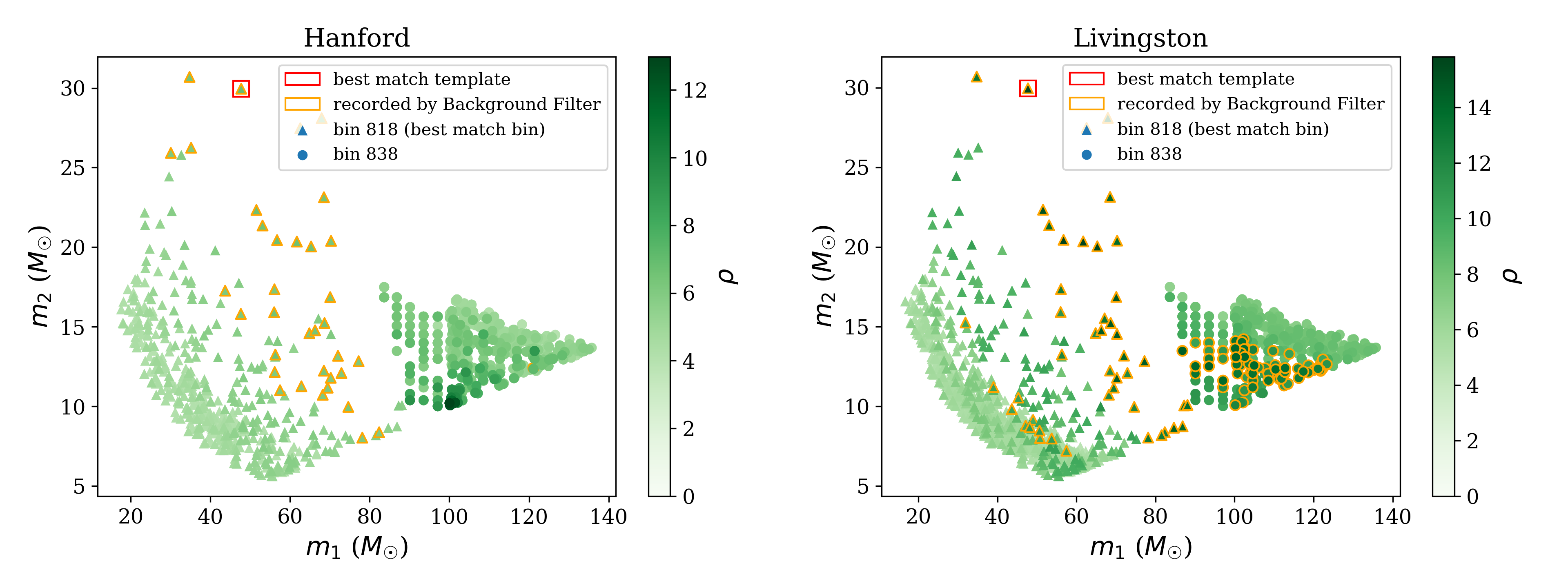
Figure 1: An example of an event (GW200129_065458) having templates with high match in multiple template bins. Bin 818 has the best match with the GW candidate, and recovers it in both Hanford and Livingston as a coincidence. Bin 838 has a lower match than bin 818, causing it to recover the candidate as a Livingston single. This will lead to the candidate being added to the $\rho-\xi^{2}$ background histogram of bin 838, causing signal contamination for bin 838. This is shown in Fig. 3. The events passing the $\rho$ and $\xi^{2}$ constraints, and hence recorded by the Background Filter are outlined in orange.

III Removing contamination with the Background Filter

To prevent any loss in sensitivity due to signal contamination, we need to selectively remove the events in the $\rho-\xi^{2}$ background histograms which originate from GW signals. The Background Filter is a way to track the background in a time-dependent fashion so that we only use events from times not corresponding to GW events to populate the background histograms. In this paper, we will describe the working of the Background Filter when GstLAL is running in the low-latency online mode, in which data is analyzed and results are produced in near real time Ewing et al. (2023).

III.1 Recording events

The strategy of the Background Filter is to record the events that are likely to have originated from GW signals, and then after verification by the user, subtract them from the background histograms. To associate events with a GW candidate, we need to record the time at which they were found in the data, apart from their $\vec{\rho}$ and $\vec{\xi^{2}}$ values. This increases the dimensionality of the parameters we need to store, and thus could potentially impact the memory and storage used during analysis. To prevent this, we record events only if they pass certain constraints placed on their $\rho$, $\xi^{2}$, and time parameters.

The $\rho$ and $\xi^{2}$ constraints take the form of a bounding box in $\rho-\xi^{2}$ space, defined by $\rho>6$ and $\xi^{2}/\rho^{2}<0.04$. Qualitatively, $\xi^{2}$ represents how well the data fits the template, with large values of $\xi^{2}$ meaning the data is dissimilar to the template. Since in general, noise events will not fit the template well, they generally have $\xi^{2}/\rho^{2}$ values that are greater than those of signals. As a result, we only expect events originating from GW signals to fall inside the bounding box. This is shown in Fig. 1, where most of the high $\rho$ events caused by GW200129_065458 pass the $\rho$ and $\xi^{2}$ constraints, and are recorded by the Background Filter. The $\rho$ and $\xi^{2}$ constraints are shown on top of a background histogram in Fig. 3

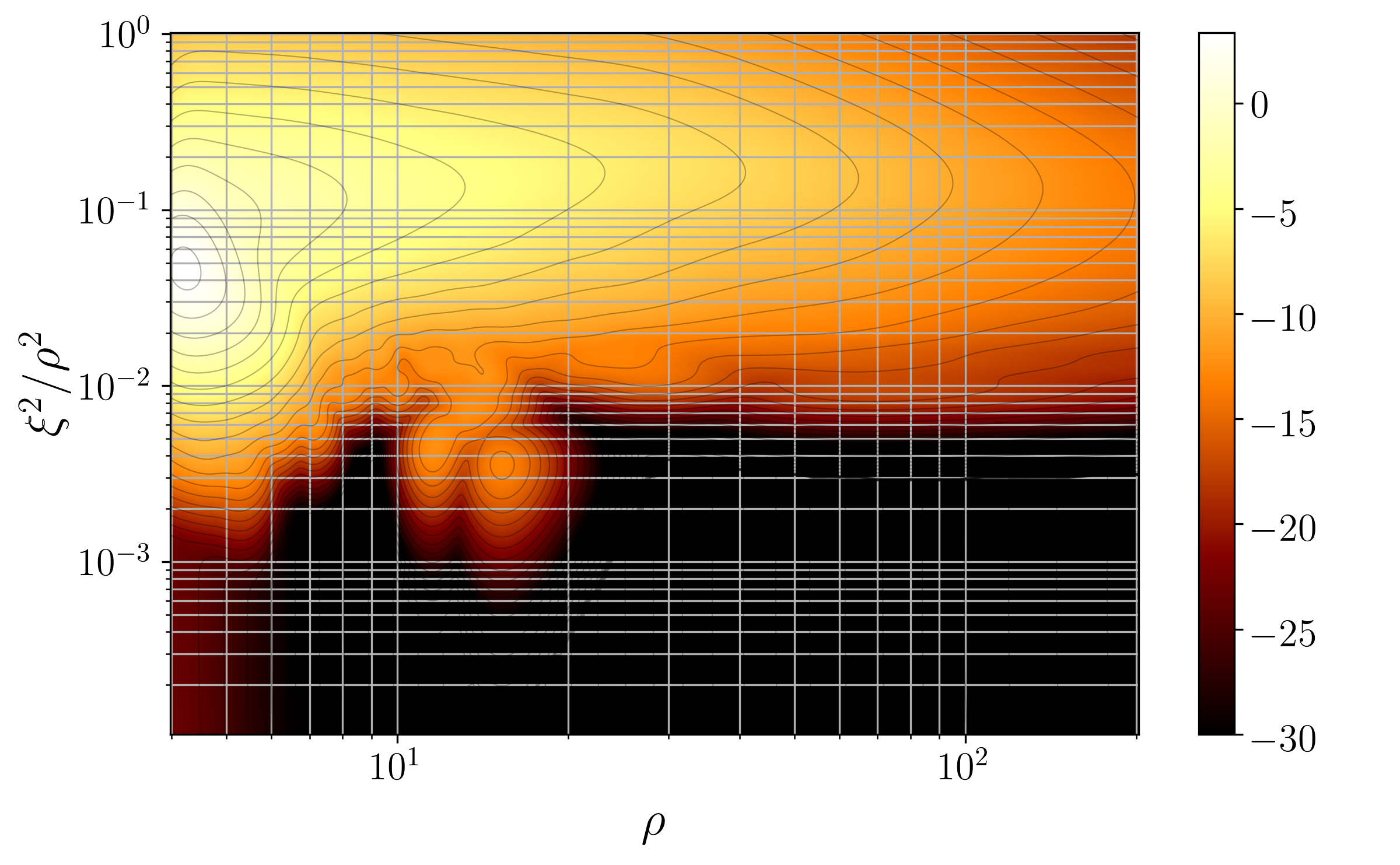
Figure 2: An example of signal contamination in a $\rho-\xi^{2}$ histogram for Livingston. The contamination can be seen as a protrusion to the histogram at ($\rho$, $\xi^{2}/\rho^{2}$) $\sim$ (15, 0.004), a region ususally occupied exclusively by GW signals. This contamination was caused by GW200129_065458 being recovered as a single event in this template bin, which is not the best match bin for that GW candidate, as demonstrated in Fig. 1. Note that kernel smoothing has been applied to this histogram.

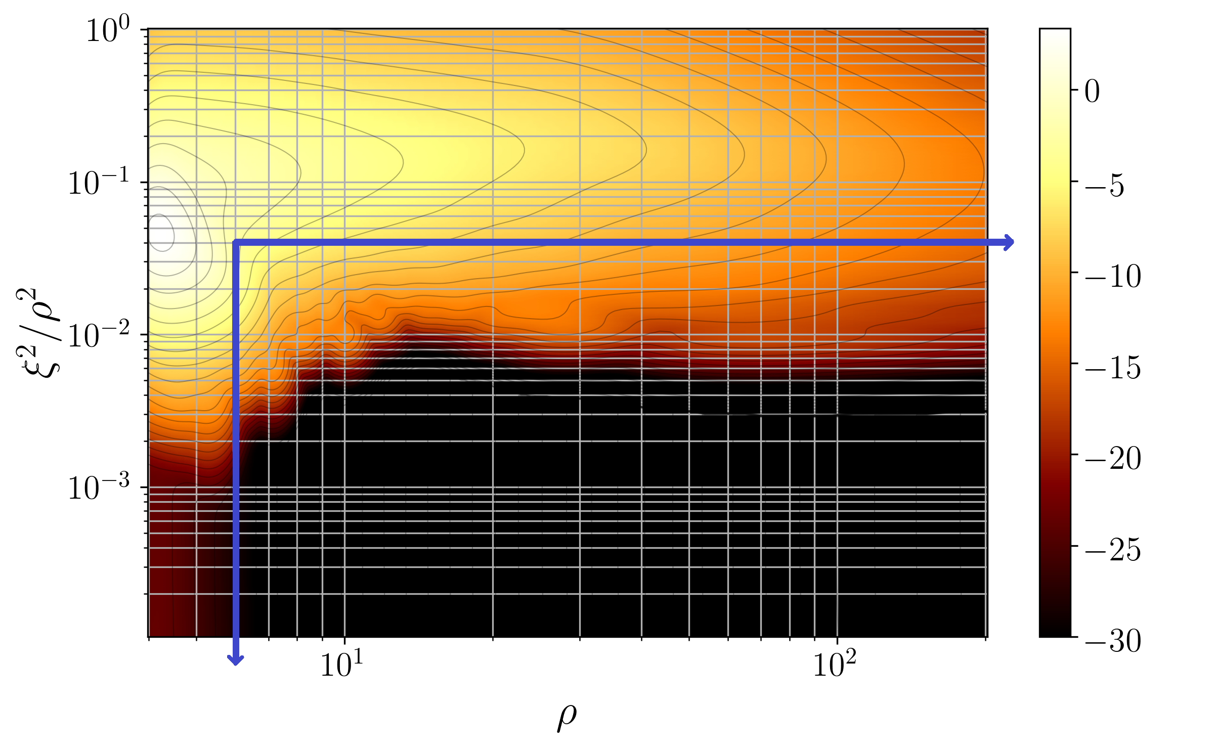
Figure 3: The $\rho$ and $\xi^{2}$ constraints for recording events. The bottom right area bounded by the blue lines is the area in which the Background Filter records events. If the events also pass the time constraint, the user can choose to remove them from the $\rho-\xi^{2}$ histogram. The result of doing so, to remove the contamination caused by GW200129_065458 is also shown. The same histogram, without using the Background Filter, and hence with contamination is shown in Fig. 3. Note that kernel smoothing has been applied to this histogram.

The time constraint makes use of the GstLAL online analysis’ ability to process data, generate events, assign LRs, and upload them to the Gravitational Wave Candidate Event Database (GraceDB) Moe et al. (2014) in near real time. A GW signal can create multiple contaminating events across template bins. Only a small subset gets uploaded to GraceDB, since the events are aggregated within some time window across bins before uploading Ewing et al. (2023), and the remaining comtaminating events lie both before and after the uploaded events in time. With this in mind, and in order to account for processing delays during a GstLAL online analysis, the Background Filter keeps a temporary record of events passing the $\rho$ and $\xi^{2}$ constraints, which occurred in the last 5000s. When an event is uploaded to GraceDB, the events in the 10s window around it are found from the temporary record of the last 5000s, and are then recorded by the Bakground Filter permanently.

The threshold for uploading an event to GraceDB differs among different GstLAL analyses, but it is often set to False Alarm Rate (FAR) $<$ 1 per hour. That means all events recovered as a single event during coincident time, with $\rho>6$, $\xi^{2}/\rho^{2}<0.04$ and falling in a 10s interval around an event with FAR $<$ 1 per hour are recorded by the Background Filter.

The $\rho$ and $\xi^{2}$ constraints, and the time constraint work together to ensure that only events originating from GW signals are recorded by the Background Filter in most cases. As a result, very few events are recorded by the Background Filter, in comparison to the number of events in the background histograms. This ensures that adding the Background Filter to a GstLAL analysis does not affect its memory or disk usage significantly. The choice of these constraints, and their impact on the performance of a GstLAL analysis are discussed in Appendix A.

III.2 Removing contamination

As explained in Sec. II, since the $\rho-\xi^{2}$ noise LR term is calculated by evaluating the probability density function represented by the background histrgrams at the relevant ($\vec{\rho}$, $\vec{\xi^{2}}$) value, we need the background histograms to accurately reflect the detector noise characteristics for that template bin. As much as possible, we need to take care not to let events originating from signals enter the background histograms. In addition, we must also make sure that events originating from noise are not removed from the background histograms by the Background Filter. In most cases, the $\rho$ and $\xi^{2}$ constraints along with the time constraint are sufficient to ensure only events originating from signals are recorded by the Background Filter.

However, in rare cases, such as when the GstLAL analysis uploads a false positive to GraceDB (also called a “retraction”), these measures might not be enough. Out of an abundance of caution, we leave the decision of which events to remove from the background histograms to the user. At any point during a GstLAL online analysis, the user can choose to inform the analysis which events they are confident are GW candidates. The message is communicated to the analysis in real time using HTTP request methods, with the help of the Python Bottle module bot . Then, out of all the events that had been recorded by the Background Filter previously, it will subtract those which fall within a 10s window of the given candidate, from the background histograms. Thus, any contamination that that candidate could have potentially caused is removed, and the LR of all future events is evaluated using the modified $\rho$ - $\xi^{2}$ background histograms.

In Fig. 3, signal contamination caused by GW200129_065458 is shown. The same $\rho$ - $\xi^{2}$ histogram, but with the Background Filter used to remove that contamination is shown in Fig. 3.

IV Results

IV.1 Analysis methods

To test the effect of signal contamination on the sensitivity of a GstLAL analysis, and the ability of the Background Filter to remove the contamination, we analyze a week of O3 data The LIGO Scientific Collaboration et al. (2023), from Apr 18 2019 16:46 UTC to Apr 26 2019 17:14 UTC, in three different ways. First, we perform a control run without any GW signals. Next, to simulate the effect of GW signals, we add “blind injections”. The concept of blind injections, and the set of blind injections that we used are explained in the following subsection. Finally, we perform a “rerank” with the Background Filter enabled, in which LRs are recomputed and significance assignment is done again, but the filtering stage of the GstLAL analysis is taken from the blind injection analysis, since the $\rho$ and $\xi^{2}$ values of analyzed events are not affected by the Background Filter, only the LRs and the False Alram Rates (FARs) are. Hence, the rerank corresponds to the case with blind injections present, and the Background Filter being used.

An important point to note is that since we are using blind injections to replicate the effect of GW signals, we know with certainty the times when GW signals will occur. This allows us to use the Background Filter on all those times, thus presenting a best-case scenario for the efficacy of the Background Filter.

This chunk of data contains two known GW candidates reported in GWTC-2.1 The LIGO Scientific Collaboration et al. (2021) and elsewhere Abbott et al. (2020, 2021a), GW190421_213856 and GW190425. However, since we use the Background Filter only on the times of the blind injections, any contamination and subsequent loss in sensitivity caused by either of the two candidates will be present in all three analyses that we perform, and will not affect the evaluation of the performance of the Background Filter.

IV.2 Simulation Set

Blind injections are simulated GW signals that are added to the data which we analyze and collect background events from (in contrast to regular injections, from which we do not collect background events). We use a set of 868 blind injections distributed across the binary black hole (BBH), binary neutron star (BNS), neutron star-black hole (NSBH), and intermediate-mass black hole (IMBH) parameter spaces. The blind injection set comprises of three subsets, a BNS subset, a BBH subset and a broad subset, with the BNS subset containing half of the total blind injections, and the BBH and broad subsets containing a quarter each. The BNS subset has component masses distributed uniformly from 1 to 3 $M_{\odot}$, and the z-components of dimensionless spin (which are parallel to the orbital angular momentum of the binary) distributed uniformly from -0.05 to 0.05. The BBH subset has component masses distributed uniformly from 5 to 50 $M_{\odot}$ and the z-components of dimensionless spin distributed uniformly from -0.99 to 0.99. The broad subset spans all four parameter spaces mentioned above. It is distributed uniformly in the log of the component masses from 1 to 300 $M_{\odot}$ and has the z-components of dimensionless spin distributed uniformly from -0.99 to 0.99. In addition to the definitions of the BNS and BBH parameter spaces provided above, and the implied NSBH parameter space definitiion, for the purpose of this paper, we shall consider the parameter space with either component mass greater than 50 $M_{\odot}$ to be the IMBH space. The distribution of the blind injection set in the two component masses can be seen in Fig. 4.

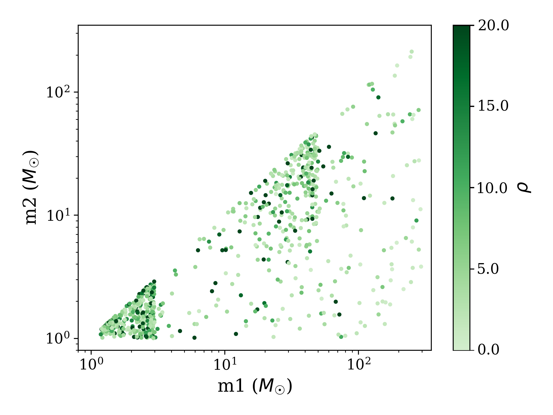
Figure 4: The distribution of component masses of the blind injection set, colored by injected $\rho$. Blind injections are used to replicate the contamination caused by GW signals in the data.

A point to note is that even though 868 blind injections may sound high, most of these are too quiet to be recovered, as shown in Fig. 4, and hence won’t cause any contamination. The result of the analysis shows that only $\sim$ 200 blind injections are loud enough to be recovered. We will also see later that BNS and NSBH template bins are not affected by signal contamination to a significant degree. As a result, only the BBH and IMBH injections will contribute to contaminating the background. Given the high number of GW candidate events we expect to detect in O4, this is a reasonable representation of the total amount of signal contamination we expect to see.

We also perform an injection campaign to calculate the sensitivity of the analysis, both with and without the application of the Background Filter. The injection set is distributed similarly to the blind injection set, but with a total size of 86,606 injections. It is important to note that the injections and blind injections are analyzed separately, with the blind injections affecting injection recovery only through the background events they add to the $\rho$ - $\xi^{2}$ background histograms.

IV.3 Sensitivity Improvements

In order to estimate the sensitivity of a search, we use the sensitive volume-time (VT) as a measure. The volume that we analyze is determined by the efficiency of recovering injections at a given FAR and redshift, and T is the livetime of the analysis. We calculate VT separately for injections falling in four different chirp mass bins. The first is from 0.5 to 2 $M_{\odot}$, the second from 2 to 4.5 $M_{\odot}$, the third from 4.5 to 45 $M_{\odot}$, and the final one is from 45 to 450 $M_{\odot}$. The reason for calculating VT separately for different mass bins is so that we have an idea about how sensitive the analysis is for different source categories, with the four mass bins roughly corresponding to BNS, NSBH, BBH and IMBH source categories respectively.

Comparing the blind injection analysis with the control run, signal contamination due to the presence of blind injections causes a small ($\sim$ 5%) decrease in VT in the two lowest mass bins, but causes a significant ($\sim$ 20-30%) decrease in VT in the two highest mass bins. This is shown in Fig. 5. High mass templates have a greater match with their neighbouring templates, and with themselves across time, as compared to low mass templates. We hypothesize that this causes a single high mass GW signal to be recovered multiple times across template bins and time with suboptimal $\rho$, leading to more signal contamination in the high mass template bins than in the low mass ones. This is discussed in more detail in Appendix B.

Figure 5: The decrease in VT caused by signal contamination due to the presence of blind injections in the data. The two highest mass bins are the most affected. The presence of GW signals will also have a similar effect.

Next, to check the efficacy of the Background Filter in removing contamination, we compare the VT of the rerank to the VT of the control run. Despite the presence of blind injections in the data, The Background Filter mitigates the effect they have on the background histograms, and sensitivities of all four mass bins are essentially the same as what they were in the control run. This is shown in Fig. 6. This represents a 20-40% increase in the sensitivities of the two high mass bins, in the case of the rerank, as compared to that of the blind injection analysis. We can conclude that in the best case, the Background Filter is successful in removing all the contamination that the blind injections cause. Since the number of blind injections we used was a high estimate of the number of GW events we expect to see in O4, this means that by using the Background Filter, we do not expect signal contamination to be a significant problem during O4. To test our readiness for O4, GstLAL has participated in a mock data challenge, where an online analysis is run over forty days of O3 data Ewing et al. (2023). The Background Filter was deployed in this analysis, and it was able to remove all instances of signal contamination.

Figure 6: The VT of the rerank, which has blind injections with the Background Filter applied, compared to that of the control run, which has neither. The fact that all four lines are close to 1 tells us that the Background Filter is successful in removing close to all of the contamination caused by the presence of the blind injections in the data. The peaks and dips in the highest mass bin curve are explained by the smaller number of injections in this bin as compared to other bins, leading to greater variance.

V Conclusion

GstLAL constructs $\rho$ - $\xi^{2}$ background histograms to calculate the $P\left(\vec{\rho},\vec{\xi^{2}}\mid t_{\mathrm{ref}},\bar{\theta},\mathcal{H}_{\mathrm{n}}\right)$ term in the likelihood ratio. However, GW signals in the data can cause the background histograms to be incorrectly constructed. This is called signal contamination, and it leads to the sensitivity of the GstLAL analysis being lowered.

The Background Filter is a novel way to remove the contamination. It records the events that populate the background histograms which satisfy two constraints. The first is that the event must fall in an area in $\rho$ - $\xi^{2}$ space consistent with GW signals. The second is that it must fall in a 10s window around a significant event. The user then identifies which of the significant events originate from GW signals. The user communicates this to the GstLAL analysis in real time, and then the events recorded by the Background Filter corresponding to the times identified by the user are subtracted from the background histograms. Thus, signal contamination is removed from the background histograms.

To test the efficacy of the Background Filter, we ran a GstLAL analysis over a week of O3 data, with simulated gravitational-wave signals injected into the data. We found that signal contamination primarily affects the high mass bins. The sensitivity of these bins decreased by 20-30% due to the presence of the gravitational-wave signals. By applying the Background Filter, we were able to increase the sensitivity back to what it was without the injected gravitational-wave signals. This shows that the Background Filter is effective in removing close to all the signal contamination. With a high rate of gravitational-wave events expected during O4, the Background Filter will be an important tool in improving the sensitivity of the GstLAL analysis.

Appendix A Choice of constraints, and their impact on performance

With the constraints described in Sec. III, the Background Filter does not consume too many resources. When looking at a month-long GstLAL analysis, we found that on average, it adds $\sim$ bytes to kilobytes to the data products stored by a GstLAL analysis for every template bin. We didn’t see any significant increase to the memory used by the GstLAL analysis either. Fig. 6 shows that with these constraints, the Background Filter is effective in removing close to all contamination.

To check if there is any improvement to the sensitivity upon loosening the $\rho$ and $\xi^{2}$ constraints, we performed the same analysis as described in Sec. IV, but with the $\rho$ and $\xi^{2}$ constraints changed to record events with $\rho>6$ and $\xi^{2}/\rho^{2}<0.4$. This broader bounding box for recording events did not have any noticeable effect on the sensitivity. This is shown in Fig. 7. However, loosening the constraints did increase memory usage of the GstLAL analysis to a noticeable degree.

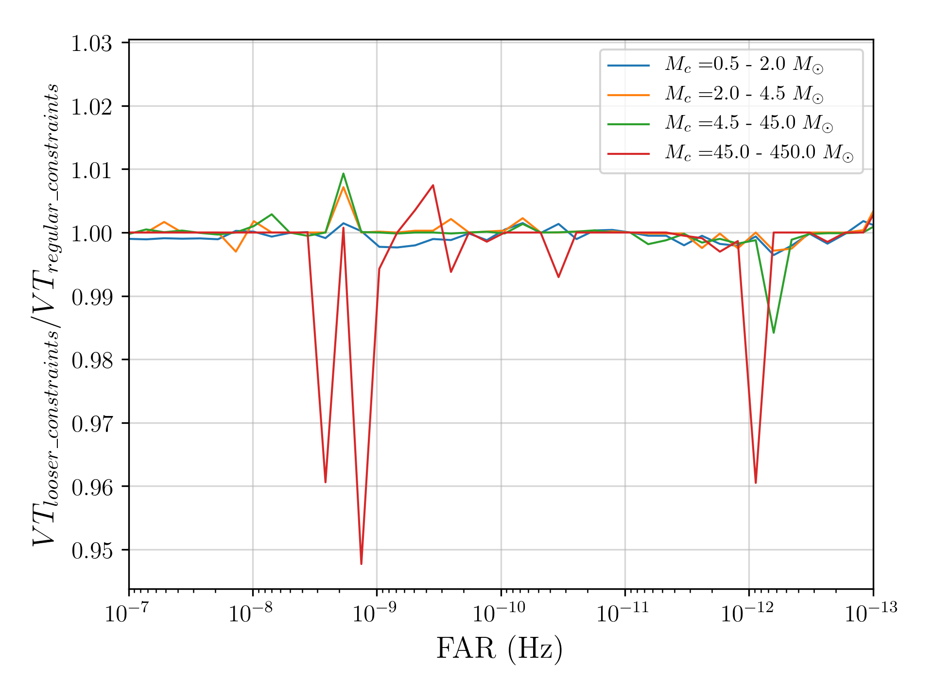
Figure 7: The VT with the Background Filter recording events with looser constraints, as compared to the VT with the Background Filter recording events with the regular constraints. The fact that the VT ratios for all four mass bins are close to 1 shows that loosening the constraints does not improve sensitivity. The peaks and dips in the highest mass bin curve are explained by the smaller number of injections in this bin as compared to other bins, leading to greater variance. Both analyses included the 868 blind injections described in Sec. IV. The regular constraints are described in Sec. III, whereas the looser constraints are described in Appendix A.

We do not expect that loosening the $\rho>6$ constraint or the time constraint would increase sensitivity, since the extra events collected by changing these constraints would be no more significant than noise. This discussion, along with Fig. 6 show us that the existing constraints used by the Background Filter satisfy all our requirements.

Appendix B Differing impacts of singal contamination of the sensitivities of template bins

As discussed in Sec. IV, signal contamination only causes a 5% decrease in the VT of low mass template bins, such as the BNS and NSBH bins, whereas it causes a 20-30% decrease in the VT of high mass template bins, such as the BBH and IMBH bins. This is despite the fact that there are more blind injections in the low mass parameter spaces than in the high mass ones. We conjecture two reasons for this, the first relating to how the correlation among neighbouring templates changes with mass, and the second relating to how the correlation of a templates with itself across time changes with mass. For the remainder of this section, we shall treat BNS template bins as representative of all low mass bins, and IMBH template bins as representative of all high mass bins.

The “bank correlation function” of a template measures how well it matches with other templates in the template bank. This calculation is similar to how $\rho$ is calculated, except that the match is calcualted between two templates with no time shift between them. To see how the bank correlation function of templates changes with mass, we took 5 BNS template bins (corresponding to $\sim$ 5000 templates), calculated the bank correlation of every combination of templates, and plotted the average bank correlation function in descending order of template match. We then did the same for 5 IMBH template bins. The results are shown in Fig. 8. The fact that the BNS bank correlation function drops sharply as compared to the IMBH one, means that there are many IMBH templates, across template bins that can recover a given IMBH GW signal with a lower $\rho$ than the best template, but only a few BNS templates that can recover a given BNS GW signal. This means a high mass GW signal will create many events, increasing the probability of signal contamination. This is not a problem for the GW candidates reported by GstLAL, since “event clustering” Messick et al. (2017) ensures that only the best candidate in an 8s window survives.

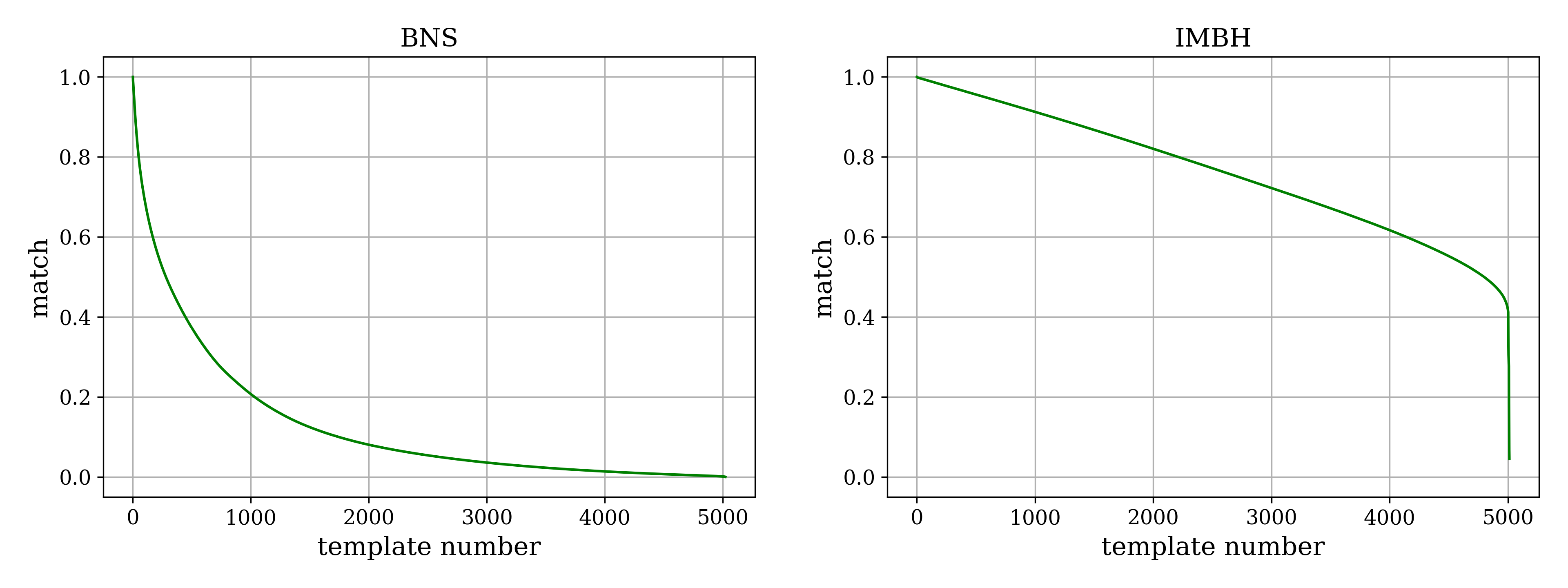
Figure 8: The average bank correlation function of a BNS template in descending order of template match, as compared to that of an IMBH template, calculated for the five closest template bins. Since IMBH templates correlate well with other IMBH templates across template bins, an IMBH GW signal will be recovered by multiple template bins, increasing the probability of signal contamination. This is not the case for BNS template bins, and it is more likely a BNS GW signal will be recovered by only one template bin, resulting in fewer cases of signal contamination.

The “autocorrelation function” of a template measures how well it matches with a time-shifted version of itself, similar to how $\rho$ calculates the match between the data and a time-shifted template. The autocorrelation function of a typical BNS template and a typical IMBH template are shown in Fig. 9. The IMBH autocorrelation function has multiple secondary peaks $\sim$ 5-10ms away from the primary one. We conjecture that in the case of an IMBH GW singal with low $\rho$ or in high noise, an IMBH template could recover the signal in different detectors at different times, corresponding to the different peaks in the IMBH autocorrelation function. This would cause the signal to be recovered as multiple single detector events, instead of a single coincident one, leading to signal contamination of the high mass template bins. Again, this is not a problem for the GW candidates reported by GstLAL, due to event clustering. Since all the secondary peaks in the autocorrelation function of an IMBH template lie well within an 8s window, multiple single detector events will be clusterd out, and only the best one will survive.

For high mass bins, the bank correlation factor increases the probability of low $\rho$ events getting created by a GW signal, and the autocorrelation factor increases the probability of signal contamination from those events. These two factors compound each other’s effect, and as a result, we see a much higher impact of signal contamination in the high mass template bins than in the low mass ones.

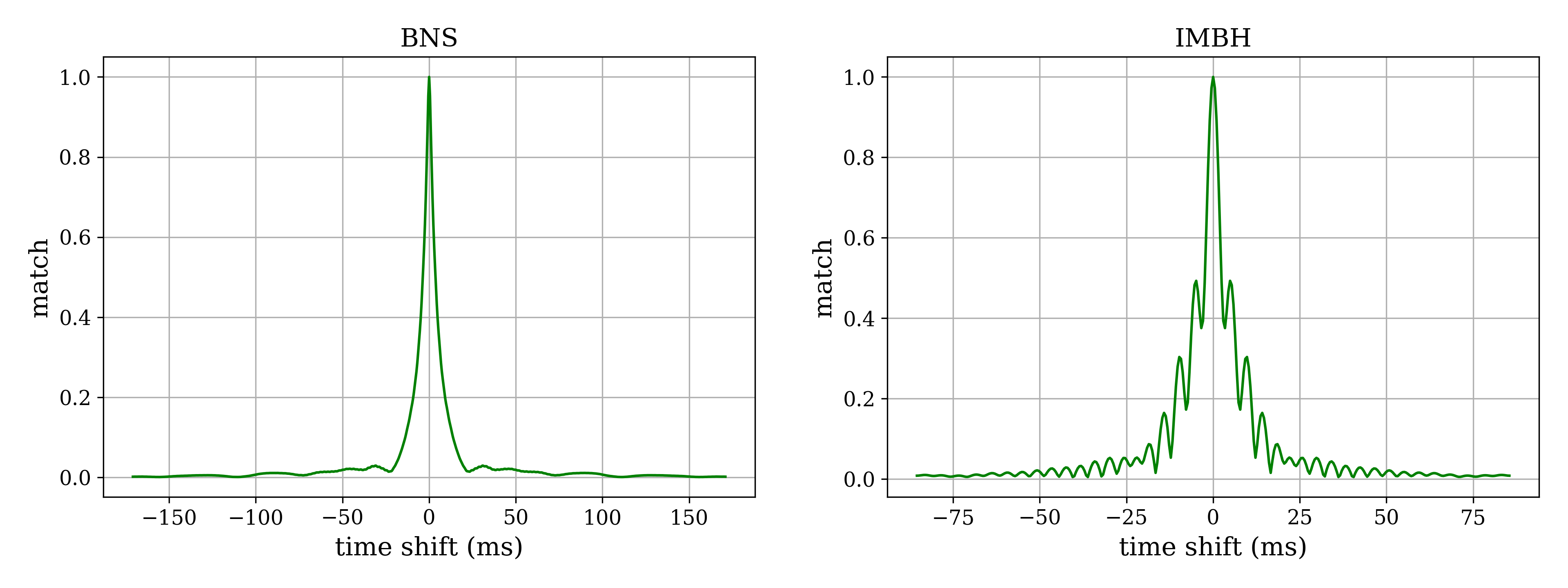
Figure 9: The autocorrelation function of a BNS template, as compared to that of an IMBH template. Since there are multiple peaks in autocorrelation function of the IMBH template, a quiet IMBH GW signal could be recovered in different detectors at different times, corresponding to the different peaks in the IMBH autocorrelation function. This will result in the GW singal being recovered as multiple single detector events rather than a single coincident event, which leads to signal contamination. Since the BNS autocorrelation function does not have multiple peaks, signal contamination is less likely for BNS template bins.

References

- Aasi et al. (2015) J. Aasi et al. (LIGO Scientific), Class. Quant. Grav. 32, 074001 (2015), arXiv:1411.4547 [gr-qc] .
- Acernese et al. (2015) F. Acernese et al. (VIRGO), Class. Quant. Grav. 32, 024001 (2015), arXiv:1408.3978 [gr-qc] .
- Abbott et al. (2019) B. P. Abbott et al. (LIGO Scientific, Virgo), Phys. Rev. X 9, 031040 (2019), arXiv:1811.12907 [astro-ph.HE] .
- gwt (2021) Physical Review X 11, 021053 (2021).
- The LIGO Scientific Collaboration et al. (2021) The LIGO Scientific Collaboration, The Virgo Collaboration, R. Abbott, et al., “Gwtc-2.1: Deep extended catalog of compact binary coalescences observed by ligo and virgo during the first half of the third observing run,” (2021).
- Abbott et al. (2021a) R. Abbott et al. (LIGO Scientific, VIRGO, KAGRA), “GWTC-3: Compact Binary Coalescences Observed by LIGO and Virgo During the Second Part of the Third Observing Run,” (2021a), arXiv:2111.03606 [gr-qc] .
- Abbott et al. (2021b) R. Abbott et al. (LIGO Scientific, Virgo), The Astrophysical Journal Letters 913, L7 (2021b).
- Abbott et al. (2021c) R. Abbott et al. (LIGO Scientific, Virgo), Phys. Rev. D 103, 122002 (2021c).
- the LIGO Scientific Collaboration et al. (2023) the LIGO Scientific Collaboration, the Virgo Collaboration, and the KAGRA Collaboration, “Search for gravitational-lensing signatures in the full third observing run of the ligo-virgo network,” (2023), arXiv:2304.08393 [gr-qc] .
- Magee et al. (2018) R. Magee, A.-S. Deutsch, P. McClincy, C. Hanna, C. Horst, D. Meacher, C. Messick, S. Shandera, and M. Wade, Phys. Rev. D 98, 103024 (2018).
- Messick et al. (2017) C. Messick et al., Phys. Rev. D95, 042001 (2017), arXiv:1604.04324 [astro-ph.IM] .
- Sachdev et al. (2019) S. Sachdev et al., (2019), arXiv:1901.08580 [gr-qc] .
- Hanna et al. (2020) C. Hanna et al., Phys. Rev. D101, 022003 (2020), arXiv:1901.02227 [gr-qc] .
- Cannon et al. (2021) K. Cannon, S. Caudill, C. Chan, B. Cousins, J. D. Creighton, B. Ewing, H. Fong, P. Godwin, C. Hanna, S. Hooper, R. Huxford, R. Magee, D. Meacher, C. Messick, S. Morisaki, D. Mukherjee, H. Ohta, A. Pace, S. Privitera, I. de Ruiter, S. Sachdev, L. Singer, D. Singh, R. Tapia, L. Tsukada, D. Tsuna, T. Tsutsui, K. Ueno, A. Viets, L. Wade, and M. Wade, SoftwareX 14, 100680 (2021).
- (15) https://gcn.gsfc.nasa.gov/other/G298048.gcn3.
- Abbott et al. (2017) B. P. Abbott et al. (LIGO Scientific Collaboration and Virgo Collaboration), Astrophys. J. Lett. 848, L12 (2017), arXiv:1710.05833 [astro-ph.HE] .
- Akutsu et al. (2020) T. Akutsu et al., Progress of Theoretical and Experimental Physics 2021 (2020), 10.1093/ptep/ptaa125, 05A101, https://academic.oup.com/ptep/article-pdf/2021/5/05A101/37974994/ptaa125.pdf .
- Tsukada et al. (2023) L. Tsukada, P. Joshi, S. Adhicary, R. George, A. Guimaraes, C. Hanna, R. Magee, A. Zimmerman, P. Baral, A. Baylor, K. Cannon, S. Caudill, B. Cousins, J. D. E. Creighton, B. Ewing, H. Fong, P. Godwin, R. Harada, Y.-J. Huang, R. Huxford, J. Kennington, S. Kuwahara, A. K. Y. Li, D. Meacher, C. Messick, S. Morisaki, D. Mukherjee, W. Niu, A. Pace, C. Posnansky, A. Ray, S. Sachdev, S. Sakon, D. Singh, R. Tapia, T. Tsutsui, K. Ueno, A. Viets, L. Wade, and M. Wade, (2023), arXiv:2305.06286 [astro-ph.IM] .
- Cannon et al. (2015) K. Cannon, C. Hanna, and J. Peoples, (2015), arXiv:1504.04632 [astro-ph.IM] .
- Cannon et al. (2013) K. Cannon, C. Hanna, and D. Keppel, Phys. Rev. D88, 024025 (2013), arXiv:1209.0718 [gr-qc] .
- Mukherjee et al. (2018) D. Mukherjee et al., (2018), arXiv:1812.05121 [astro-ph.IM] .
- Sakon et al. (2022) S. Sakon, L. Tsukada, H. Fong, C. Hanna, J. Kennington, S. Adhicary, K. Cannon, S. Caudill, B. Cousins, J. D. E. Creighton, B. Ewing, P. Godwin, Y.-J. Huang, R. Huxford, P. Joshi, R. Magee, C. Messick, S. Morisaki, D. Mukherjee, W. Niu, A. Pace, C. Posnansky, S. Sachdev, D. Singh, R. Tapia, D. Tsuna, T. Tsutsui, K. Ueno, A. Viets, L. Wade, M. Wade, and J. Wang, (2022), 10.48550/ARXIV.2211.16674.
- Canton et al. (2021) T. D. Canton, A. H. Nitz, B. Gadre, G. S. C. Davies, V. Villa-Ortega, T. Dent, I. Harry, and L. Xiao, The Astrophysical Journal 923, 254 (2021).
- Davies et al. (2020) G. S. Davies, T. Dent, M. Tápai, I. Harry, C. McIsaac, and A. H. Nitz, Physical Review D 102 (2020), 10.1103/physrevd.102.022004.
- Nitz (2018) A. H. Nitz, Physical Review D 98 (2018), 10.1103/PhysRevD.98.024050.
- Aubin et al. (2021) F. Aubin, F. Brighenti, R. Chierici, D. Estevez, G. Greco, G. M. Guidi, V. Juste, F. Marion, B. Mours, E. Nitoglia, O. Sauter, and V. Sordini, Classical and Quantum Gravity 38, 095004 (2021).
- Adams et al. (2016) T. Adams, D. Buskulic, V. Germain, G. M. Guidi, F. Marion, M. Montani, B. Mours, F. Piergiovanni, and G. Wang, Classical and Quantum Gravity 33, 175012 (2016).
- Chu (2022) Q. Chu, Physical Review D 105 (2022), 10.1103/PhysRevD.105.024023.
- Chu (2017) Q. Chu, Low-latency detection and localization of gravitational waves from compact binary coalescences, Ph.D. thesis, The University of Western Australia (2017).
- Venumadhav et al. (2019) T. Venumadhav, B. Zackay, J. Roulet, L. Dai, and M. Zaldarriaga, Phys. Rev. D 100, 023011 (2019).
- Zackay et al. (2021) B. Zackay, L. Dai, T. Venumadhav, J. Roulet, and M. Zaldarriaga, Physical Review D 104 (2021), 10.1103/physrevd.104.063030.
- (32) “Igwn public alerts user guide:observing capabilities,” https://emfollow.docs.ligo.org/userguide/capabilities.html.
- Ewing et al. (2023) B. Ewing, R. Huxford, D. Singh, L. Tsukada, C. Hanna, Y.-J. Huang, P. Joshi, A. K. Y. Li, R. Magee, C. Messick, A. Pace, A. Ray, S. Sachdev, S. Sakon, R. Tapia, S. Adhicary, P. Baral, A. Baylor, K. Cannon, S. Caudill, S. S. Chaudhary, M. W. Coughlin, B. Cousins, J. D. E. Creighton, R. Essick, H. Fong, R. N. George, P. Godwin, R. Harada, J. Kennington, S. Kuwahara, D. Meacher, S. Morisaki, D. Mukherjee, W. Niu, C. Posnansky, A. Toivonen, T. Tsutsui, K. Ueno, A. Viets, L. Wade, M. Wade, and G. Waratkar, (2023), arXiv:2305.05625 [gr-qc] .
- Moe et al. (2014) B. Moe, P. Brady, B. Stephens, E. Katsavounidis, R. Williams, and F. Zhang, “GraceDB: A Gravitational Wave Candidate Event Database,” (2014).
- (35) “Bottle: Python web framework: https://bottlepy.org/docs/dev/,” .
- The LIGO Scientific Collaboration et al. (2023) The LIGO Scientific Collaboration, The Virgo Collaboration, The KAGRA Collaboration, R. Abbott, et al., “Open data from the third observing run of ligo, virgo, kagra and geo,” (2023).
- Abbott et al. (2020) B. P. Abbott et al. (LIGO Scientific, Virgo), (2020), arXiv:2001.01761 [astro-ph.HE] .