GazeGNN: A Gaze-Guided Graph Neural Network for Chest X-ray Classification

Abstract

Eye tracking research is important in computer vision because it can help us understand how humans interact with the visual world. Specifically for high-risk applications, such as in medical imaging, eye tracking can help us to comprehend how radiologists and other medical professionals search, analyze, and interpret images for diagnostic and clinical purposes. Hence, the application of eye tracking techniques in disease classification has become increasingly popular in recent years. Contemporary works usually transform gaze information collected by eye tracking devices into visual attention maps (VAMs) to supervise the learning process. However, this is a time-consuming preprocessing step, which stops us from applying eye tracking to radiologists’ daily work. To solve this problem, we propose a novel gaze-guided graph neural network (GNN), GazeGNN, to leverage raw eye-gaze data without being converted into VAMs. In GazeGNN, to directly integrate eye gaze into image classification, we create a unified representation graph that models both images and gaze pattern information. With this benefit, we develop a real-time, real-world, end-to-end disease classification algorithm for the first time in the literature. This achievement demonstrates the practicality and feasibility of integrating real-time eye tracking techniques into the daily work of radiologists. To our best knowledge, GazeGNN is the first work that adopts GNN to integrate image and eye-gaze data. Our experiments on the public chest X-ray dataset show that our proposed method exhibits the best classification performance compared to existing methods. The code is available at https://github.com/ukaukaaaa/GazeGNN.

1 Introduction

Image classification has always been a complicated task in the computer vision field. In recent years, because of the explosive development of machine learning techniques, deep learning-based classification algorithms have been proposed to deal with this challenging task [23, 22, 36, 12, 14, 41]. However, compared to the classical natural image datasets such as ImageNet-1k [7], medical image datasets are usually characterized by a relatively limited scale and low signal-to-noise ratio [5], which makes disease classification a more challenging task.

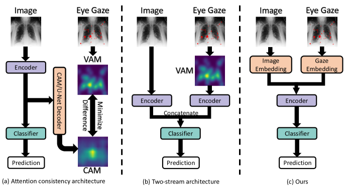
Figure 1: Illustration of our proposed method and other frameworks that integrate eye-gaze information in medical image classification.

This problem is particularly evident in chest X-ray classification. It is because chest X-ray has limited soft tissue contrast, containing a variety of complex anatomical structures overlapping in planar (2D) view [29]. Many tissues, such as organs, blood vessels, and muscles, have similar intensity values on the chest X-ray images [32]. This can easily confuse the deep learning model to distinguish between normal and abnormal tissues, making it difficult to identify the true location of abnormalities accurately.

Therefore, deep learning algorithms encounter difficulties in accurately identifying abnormality based solely on chest X-ray images. To overcome this challenge, many recent studies have applied eye-tracking techniques to complement the model with prior knowledge of the location of abnormality regions. Eye-tracking techniques collect eye-gaze data from radiologists during screening procedures [37, 38]. This eye-gaze data represents the search pattern of radiologists for tumors or suspicious lesions on the scans. It indicates the location information that radiologists have fixations and saccades on the images during diagnostic screenings. Since these positions are highly likely to hold abnormality and potentially important regions, eye-gaze data can provide extra location information of the disease that is often challenging to be observed from medical images alone. This supplementary information, a high-level attention, can guide the deep learning model to learn the disease feature in an interpretable way. Hence, embedding eye-gaze information into diagnostic analysis has become a popular topic in recent years [2, 20, 21, 37].

The prior mainstream works on this topic can be broadly categorized into two approaches. The first one [3, 42, 18, 44, 8, 46, 33, 39] is referred to as the attention consistency architecture, illustrated in Fig. 1(a). It calculates the attention map based on the model learned by image. At the same time, eye gaze is utilized to supervise the attention map generated by the model. This ensures that the model’s attention aligns closely with the attention patterns observed by human experts. However, since this architecture only utilizes eye gaze during training as a supervision source and excludes it during testing, there is a potential risk in classification performance and model robustness. This is related to the inherent variability in eye-gaze data. The eye-gaze data can differ significantly from case to case since each radiologist may have their own unique search patterns. This individualized nature of eye-gaze data may introduce inconsistencies that complicate the learning process for classification models. Therefore, it is challenging to learn a generalized model to capture standardized eye-gaze data patterns for one specific disease. In section 4.4, we verify that attention consistency architecture exhibits poor model robustness and has a remarkable performance drop when distribution gaps exist in the data. This motivates us to study other structures to integrate eye-gaze information.

The second approach  [27, 28, 31, 18] is known as the two-stream architecture, as depicted in Fig. 1(b). It consists of two branches dedicated to processing the image and eye gaze information separately. These branches extract features from their respective sources, which are then concatenated and fed into the classification head. In the end, the predicted probabilities of each disease class are achieved. However, since the eye-gaze data consists of a group of fixation points, which is not a regular grid or sequence representation, two-stream architecture transforms the eye-gaze data into visual attention maps (VAMs) and then integrates the VAMs with the medical images. It is not ideal for real-world clinical practice because it is time-consuming to generate VAM for each image during inference ($\sim$10s for each image). There is still a need to prepare all the VAMs in advance before sending them into the network one by one. As a result, this hinders the practical application of eye tracking techniques in the daily clinical workflow.

Therefore, to address the problems of the existing two architectures, we develop a new framework illustrated in Fig. 1(c). We consider eye gaze as the model input to enhance the model robustness and directly utilize the raw eye-gaze data without converting it to the VAMs to improve time efficiency. To bypass the usage of VAM and fully integrate eye gaze with image, we apply a graph to model multiple information in a single representation and adopt the Graph Neural Network (GNN) to learn the graph. Unlike the nowadays’ widely sought Transformer model, GNN is shown to be highly effective even with limited training data, making it a better choice for medical settings [10]. Additionally, GNN has the advantage of capturing the relational information between different parts of the image according to their semantic and categorical attributes [11]. This capability facilitates the learning of relationships between various organs and even the distinction between normal and abnormal regions within the image.

To adapt GNN for disease classification, the image is divided into patches to construct a graph. In the graph, each node stands for a feature fused from three types of information: the location of the patch in the image, the local intensity information of the image patch, and the human attention information from the patch. Respectively, we employ three different embedding techniques to encode the information respectively: (i) positional embedding for the location of the patch, (ii) patch embedding for patch local intensity values extraction, and (iii) gaze embedding for aggregating the fixation time of radiologists on the patch. Then, for each patch, the three embedding features are combined as a single feature vector. Finally, each node is connected to its $k$-nearest neighbors to build the graph. By feeding the graph into a GNN, we obtain the disease classification model.

The major contributions of this work are summarized as:

1. We propose a novel Gaze-guided GNN framework, GazeGNN, which can directly integrate raw eye-gaze data with images, bypassing the need to convert gaze into VAMs. This reduces the inference time of each case from $\sim$10s to less than 1s, making it the first study that can be applied to real-world clinical practice due to its efficiency and seamless integration.

2. We leverage the flexibility of a graph network to design a unified graph representation that can encode multiple types of information - the location of the patch in the image, the local intensity information of the image patch, and the human attention information focused on the patch - within a single representation.

3. Rather than a supervision source, we verify incorporating eye-gaze data as a model input that can enhance the model’s robustness and reduce performance drop in scenarios where distribution gaps exist.

4. By evaluating GazeGNN on a public chest X-ray dataset [18], our proposed method achieves the state-of-the-art performance on the disease classification task. It outperforms the existing strategies that utilize both image and eye-gaze data, from the perspectives of accuracy, robustness, and time efficiency.

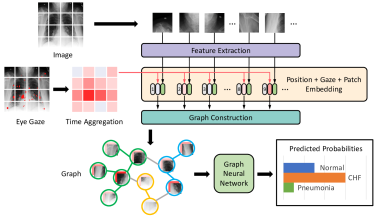
Figure 2: An overview of our proposed GazeGNN framework. It includes a graph construction based on patch, gaze, and position embeddings and a graph neural network for disease classification.

2 Related Works

2.1 Chest X-ray Classification

Chest X-ray classification has witnessed significant advances in recent years with the power of large-scale public chest X-ray datasets and advanced machine learning techniques. Large-scale chest X-ray datasets such as CheXpert [15], MIMIC-CXR [17], ChestX-ray14 [30], and others [4, 45, 6, 19] have significantly contributed to the model training and evaluation. These datasets provide nearly a million of chest X-ray images (in total) with class annotations, enabling the development of chest X-ray classification algorithms developments. On the other side, the development of advanced deep learning algorithms has enhanced the accuracy and performance of chest X-ray classification. Most methods are mainly based on chest X-ray images and propose new network architectures to conduct the analysis [30, 16, 1, 35, 9]. Very recently, studies have started to explore the eye-gaze data on chest X-ray classification task [18, 42, 39]. Research has shown that the inclusion of additional human expert knowledge via eye-gaze patterns can significantly enhance the accuracy of deep learning models.

2.2 Integration of Eye-gaze Data in Medical Image Analysis

The prior mainstream works commonly transform the eye-gaze data into VAMs. A VAM is an image that highlights radiologists’ attention regions on the corresponding medical image. Related works can be generally divided into two categories based on their utilization of the VAMs. The first category considers the VAMs as a part of the input for the network models. For example, in [27, 28, 31], authors apply VAMs to process the images and take the processed images as the model input. In [18], authors employ a CNN-LSTM hybrid two-stream neural network, where the CNN is used to process the medical images, and the LSTM is used to encode the VAMs. The second category minimizes the difference between VAMs and class activation maps (CAMs) [3, 42] or the difference between VAMs and the attention maps generated by a U-Net decoder [18, 44].

More recently after the release of Segment Anything Model (SAM) by Meta, a human-computer interaction system, GazeSAM [40], is proposed. Basically, it combines eye tracking technology with SAM and enables users to segment the object they are looking at in real-time, which noticeably proves the possibility of bringing real-time eye gaze integration into routine clinics.

3 Method

In this section, we describe the framework of the proposed GazeGNN for the disease classification task. As illustrated in Fig. 2, GazeGNN constructs a graph from an image and eye-gaze data. Each node in the graph is represented as a combination of features through patch, gaze, and position embedding. After graph is constructed, a graph neural network is applied to update and aggregate the information of all the nodes in order to produce a feature representing the whole graph. By performing graph-level classification, we can obtain the predicted class for the input image.

3.1 Graph Representation

Our proposed GazeGNN method takes two distinct data types as input: the chest X-ray image and the corresponding eye-gaze information. The image is a regular grid structure data, while eye-gaze information is a group of scatter points that indicates the attention locations of radiologists during their evaluation process. To integrate both types of information effectively, we employ following techniques to embed them into feature vectors to construct a graph accordingly.

3.1.1 Patch Embedding

The image input size in this task is $224\times 224$. Therefore, if we treat each pixel as an individual node, there will be 50,176 nodes in the graph. This is an excessive number and makes the GNN training difficult. Instead, we divide the image into multiple $15\times 15$ patches and consider each patch as a node.

Given an image $\mathcal{I}\in\mathbb{R}^{H\times W}$, we split it into $N$ patches $\mathcal{P}=\{p_{1},p_{2},...,p_{N}\}$, where $p_{i}\in\mathbb{R}^{S\times S}$ for $i=1,2,...,N$. For each patch $p_{i}$, we extract a feature vector $\mathbf{x}_{i}^{(I)}\in\mathbb{R}^{D}$ that encodes the local image information, which is:

$$\mathbf{x}_{i}^{(I)}=F(p_{i}),$$ (1)

where $F(\cdot)$ is the feature extraction method. In this work, we adopt the overlapping patch embedding method [43] to extract the feature vectors from image patches.

3.1.2 Gaze Embedding

Eye-gaze data consists of many scatter points, and each of them means that the radiologists’ eyes have concentrated on this location for a moment when they were performing image reading. More importantly, eye gaze not only provides the location information but also offers the time duration for each point. As illustrated in “Eye Gaze” of Fig. 2, there are many red dots with different sizes scattered on the image. A bigger red dot indicates that the radiologist has spent a relatively longer time focusing on the corresponding area. To maintain consistency with the feature vector defined for a single image patch in Eq. (1), we perform time aggregation to get the fixation time for each patch.

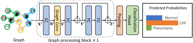
Figure 3: The architecture of the proposed Graph Neural Network (GNN).

Assume that there are $Q$ eye-gaze points $g_{(m_{1},n_{1})},g_{(m_{2},n_{2})},...,$ $g_{(m_{Q},n_{Q})}$, in which $g_{(m_{i},n_{i})}$ indicates that radiologist’s eyes fix at location $(m_{i},n_{i})$ for $g_{(m_{i},n_{i})}$ seconds. Then, to conduct the time aggregation, we sum up all the eye-gaze points’ fixation time in the patch to represent the attention feature of the patch, i.e., for each patch $p_{i}$, the gaze embedding is:

$$x_{i}^{(T)}=\sum_{(m_{j},n_{j})\in p_{i}}g_{(m_{j},n_{j})},$$ (2)

where $i\in[1,N]$ and $j\in[1,Q]$. Next, we replicate the scalar $x_{i}^{(T)}$ to the vector $\mathbf{x}_{i}^{(T)}\in\mathbb{R}^{D}$ for feature fusion.

3.1.3 Position Embedding

During the graph processing in GNN, the features are treated as unordered nodes. To keep the positional information in the original image, we adopt the position embedding method from [11], which contains two steps. The first step is to add a learnable absolute positional encoding vector $\mathbf{e}_{i}\in\mathbb{R}^{D}$ to the feature vector $\left(\mathbf{x}_{i}^{(I)}+\mathbf{x}_{i}^{(T)}\right)$. In the second step, we calculate the relative positional distance between nodes as $\mathbf{e}_{i}^{T}\mathbf{e}_{j}$, and this distance is used to determine the neighbors of a given node in the $k$-nearest neighbors algorithm for the graph construction.

3.1.4 Graph Construction

With patch, gaze, and position embeddings, the graph node feature vector $\mathbf{x}_{i}$ is elaborated as:

$$\mathbf{x}_{i}=\mathbf{x}_{i}^{(I)}+\mathbf{x}_{i}^{(T)}+\mathbf{e}_{i},$$ (3)

and these features represent the vertices $\mathcal{V}=\{\mathbf{x}_{1},\mathbf{x}_{2},...\mathbf{x}_{N}\}$. By calculating the $k$-nearest neighbors, the edges of the graph are defined as

$$\mathcal{E}=\{(\mathbf{x}_{i},\mathbf{x}_{j})\mid\mathbf{x}_{j}\in K(\mathbf{x}_{i})\},$$ (4)

where $K(\mathbf{x}_{i})$ represents the $k$-nearest neighbors of $\mathbf{x}_{i}$. In this way, a graph $G=\{\mathcal{V},\mathcal{E}\}$ is constructed.

3.2 Graph Neural Network (GNN)

As illustrated in Fig. 3, the graph neural network consists of $L$ graph processing blocks [11], an average pooling layer, and a graph classification head. Graph processing block consists of multiple fully-connected (FC) layers and a graph convolutional layer [24].

Suppose the graph is represented as $N$ $D$-dimension feature vectors. Given an input graph $\mathbf{X}^{t}=\left[\mathbf{x}_{1}^{t},\mathbf{x}_{2}^{t},...,\mathbf{x}_{N}^{t}\right]\in\mathbb{R}^{N\times D}$ at block $t$, a graph processing block outputs $\mathbf{Z}^{t}\in\mathbb{R}^{N\times D}$ as

$$\mathbf{Y}^{t}=\Psi_{2}\left(\Phi\left(\Psi_{1}\left(\mathbf{X}^{t}\right)\right)\right)+\mathbf{X}^{t},$$ (5)

$$\mathbf{Z}^{t}=\Psi_{4}\left(\Psi_{3}\left(\mathbf{Y}^{t}\right)\right)+\mathbf{Y}^{t},$$ (6)

where $\Phi$ denotes the graph convolution operation and $\Psi$ indicates FC layer. Here, we ignore the activation and batch normalization layers. Let $\mathbf{Y}^{t}\in\mathbb{R}^{N\times D}$ stand for the intermediate output after the first shortcut connection and $\mathbf{R}^{t}=\Psi_{1}(\mathbf{X}^{t})$ stand for the input of graph convolutional layer. The graph convolution $\mathbf{S}^{t}=\Phi(\mathbf{R}^{t})$ is defined as

$$\mathbf{s}_{i}^{t}\ =\mathbf{W}\cdot\max\left(\left\{\mathbf{r}_{i}^{t}-\mathbf{r}_{j}^{t}\mid j\in K\left(\mathbf{r}_{i}^{t}\right)\right\}\right),$$ (7)

where $\mathbf{S}^{t}=\left[\mathbf{s}_{1}^{t},\mathbf{s}_{2}^{t},...,\mathbf{s}_{N}^{t}\right]\in\mathbb{R}^{N\times D}$ and $\mathbf{R}^{t}=\left[\mathbf{r}_{1}^{t},\mathbf{r}_{2}^{t},...,\mathbf{r}_{N}^{t}\right]\in\mathbb{R}^{N\times D}$. $\mathbf{W}$ is a trainable weight matrix to update the feature for the node. The max term is the aggregation function that aggregates features from the $i$-th node’s neighbors. Therefore, graph convolution aggregates node neighbors’ feature information and updates it into the node feature. In the final step, the classification head is designed as a fully-connected layer with the softmax function. It outputs the predicted probability of each category.

4 Experiments

Our experiments are implemented on a workstation with an Intel Xeon W-2255 CPU and an NVIDIA RTX 3090 GPU using PyTorch. We train GazeGNN using AdamW optimizer [26] with the learning rate of 0.0001 and the batch size of 32. The checkpoint model with the best testing accuracy is saved during the training. Cross-entropy loss is used as the classification loss function. In the following experiments, we adopt [18] as the implementation of two-stream architecture and [42] as the implementation of attention consistency architecture.

Table 1: Classification results on the Chest X-Ray dataset [18].

Method	Accuracy	AUC				Precision	Recall	F1-Score
		Normal	CHF	Pneumonia	Average
Temporal Model [18]	-	0.890	0.850	0.680	0.810	-	-	-
U-Net+Gaze [18]	-	0.910	0.890	0.790	0.870	-	-	-
DenseNet121+Gaze [39]	-	-	-	-	0.836	-	-	0.270
GazeMTL [33]	78.50%	0.915	0.913	0.833	0.887	0.786	0.781	0.779
IAA [8]	78.50%	0.922	0.902	0.875	0.900	0.780	0.774	0.776
EffNet+GG-CAM [46]	77.57%	0.906	0.914	0.843	0.888	0.770	0.772	0.770
GazeGNN	83.18%	0.938	0.916	0.914	0.923	0.839	0.821	0.823

4.1 Dataset Preparation

The experiments in this paper are carried out on a public chest X-ray dataset [18], which contains 1083 cases from the MIMIC-CXR dataset [17]. For each case, a gray-scaled X-ray image with the size of around $3000\times 3000$, eye-gaze data, and ground-truth classification labels are provided. These cases are classified into 3 categories: Normal, Congestive Heart Failure (CHF), and Pneumonia. For the comparison experiments, we generate the static VAMs from the eye-gaze data using the data post-processing method as described in [18]. The model performance is evaluated through multiple metrics, including accuracy, the area under the receiver operating characteristic curve (AUC), precision, recall, and F1-score. The higher these metrics are, the better the model is. For all the experiments, we apply the same data augmentation techniques, including random resize crop into $224\times 224$, random horizontal flip, and random rotation by up to $5^{\circ}$.

4.2 Improving Disease Classification Accuracy

We compare GazeGNN with the state-of-the-art methods, including temporal model [18], U-Net+Gaze model [18], and DenseNet121-based model [39]. These methods adopt the official training and test datasets, so we directly include their reported results in this paper. We also compare GazeGNN with some other gaze-guided methods, which have not been validated on this dataset yet, or have used this dataset but did not follow the official splitting strategy. These methods include GazeMTL [33], IAA [8], and EffNet+GG-CAM [46]. To make the comparison fair, we train these methods under the same setting as GazeGNN.

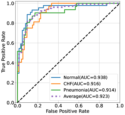
(a)

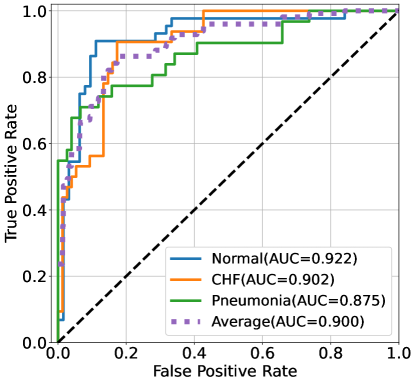
(b)

Figure 4: Comparisons of ROC curves and AUC scores

The quantitative results are summarized in Table 1. Although we primarily compare the accuracy metric in this work because we save the checkpoint models with the best testing accuracy, it is noted that the proposed GazeGNN still achieves the best performance on all the evaluation metrics. Moreover, Fig. 4 shows receiver operating characteristic (ROC) curves of the comparison method with the best average AUC and our GazeGNN. The ROC curves of other compared methods are presented in the supplemental materials.

4.3 Improving Inference Speed

Eye-gaze data is composed of a group of scatter points, indicating the location coordinates of the radiologists’ gaze on the medical image. It is not a regular grid or sequential data format. To align the eye-gaze data with the medical image, existing methods typically transform the eye-gaze into the VAMs for training purposes. The generation of VAM for each image can be a time-consuming process. There are two approaches to accomplish this step. One method is to apply a Gaussian distribution to each eye-gaze point and aggregate the individual distributions to obtain the final VAM. The other approach is to apply a Gaussian filter kernel to smooth the eye-gaze intensity value (duration time on a certain image location) on the whole image. Due to the large size of chest X-rays (approximately 2500x3000) and the considerable number of eye-gaze points, generating VAMs for each image requires substantial time. Consequently, existing methods often pre-generate all VAMs in advance before training or inference. This is not ideal when we want to integrate the eye-gaze into the radiologists’ daily work.

Table 2: Comparison of inference speed.

Method	Gaze	Inference Time
GazeGNN	✓	0.353s
Two-stream Architecture	✓	9.246s
Attention Consistency Architecture	2717	0.294s

Table 3: Performance comparison of our method across different backbones.

Backbone	Accuracy	AUC				Precision	Recall	F1-Score
		Normal	CHF	Pneumonia	Average
DenseNet121 [13]	71.03%	0.903	0.855	0.620	0.793	0.696	0.689	0.689
ResNet18 [12]	71.96%	0.906	0.820	0.687	0.804	0.706	0.706	0.705
ResNet50 [12]	70.09%	0.898	0.818	0.663	0.793	0.685	0.685	0.684
ResNet101 [12]	71.03%	0.852	0.862	0.756	0.823	0.703	0.705	0.703
Swin-T [25]	77.57%	0.925	0.898	0.732	0.852	0.762	0.760	0.755
Swin-S [25]	74.77%	0.911	0.873	0.728	0.837	0.733	0.735	0.733
Swin-B [25]	76.64%	0.907	0.880	0.770	0.852	0.771	0.754	0.748
GNN	83.18%	0.938	0.916	0.914	0.923	0.839	0.821	0.823

In our method, on the other hand, we bypass the process of generating VAM and propose a novel technique, called time aggregation with gaze embedding, to conduct eye-gaze integration. Due to the simple calculation inside the time aggregation, we significantly reduce the inference time, as shown in Table 2. We compare the inference speed of our method and the current two mainstream architectures. We test on 100 cases and calculate the average processing time as the inference time. For attention consistency architecture, a Gaussian filter kernel, with standard deviation $\sigma=150$, is applied to generate the VAM for each case.

From the result shown in Table. 2, we can find that two-stream architecture takes the longest inference time, around 10 seconds. This is mainly due to the time-consuming process of VAM generation. It is worth noting the GazeGNN obtains comparable inference time as attention consistency architecture. The attention consistency architecture does not require gaze input in the inference stage, while GazeGNN involves the eye-gaze. This demonstrates the efficiency of eye-gaze integration in our architecture, which points out the feasibility to bring real-time eye-tracking techniques into the radiology rooms.

4.4 Improving Model Robustness

Table 4: Comparison of performance drop when testing on the dataset with distribution shift.

Method	Performance Drop $\downarrow$
	Accuracy	Precision	Recall	F1-Score	Average AUC
GazeGNN	2.78%	1.10%	2.87%	3.97%	0.20%
ACA	13.79%	15.30%	15.63%	18.38%	4.86%

In attention consistency architecture, the eye-gaze data is considered a supervision source during training, as illustrated in Fig. 1. The inference stage of attention consistency architecture does not involve eye-gaze information. This requires the model to learn the eye-gaze pattern for certain diseases. However, the eye-gaze data is different case by case and each radiologist has his own search patterns when doing image reading. Further, even for the same radiologist’s second time reading of the same scan may show differences in eye-gaze patterns. Therefore, learning standardized eye-gaze data patterns for a specific disease is challenging, and likely not a generalizable model.

To fully utilize the power of eye-gaze information, we postulate that the model should incorporate gaze input in the inference stage. In this way, when encountering new data that exhibits a distribution shift from the original training dataset, we can still leverage the eye-gaze data to provide the model with the location information of the potential abnormality. To prove this assumption, we introduce random noise to the testing dataset, creating a distribution gap from the original training dataset. We then evaluate our method and attention consistency architecture (ACA) on the original and noisy testing datasets. Based on the results presented in Table 4, it is evident that the attention consistency architecture exhibits a larger performance drop compared to our proposed method, validating our previous assumption.

4.5 Effectiveness of GNN

After combining the position, gaze, and patch embedding, we obtain a single feature that represents both image and eye gaze. In this work, the feature is used to construct a graph and processed by GNN. But it also works for other backbone architectures. We employ strong backbone networks, including DenseNet, ResNet, and Swin Transformer, and compare the performance with GNN.

The performance of our method across different backbones is shown in Table 3. The Transformer backbone does not exhibit the best performance. This might be because it suffers from limited data. In addition, we see that our method with GNN achieves the best results over all the evaluation metrics. This can be attributed to two key factors. Firstly, unlike the Transformer model, GNN demonstrates remarkable effectiveness even when presented with limited training data. The other reason is that GNN can capture and comprehend the intricate relationships between patches through graph learning.

4.6 Ablation Study of Gaze Usage

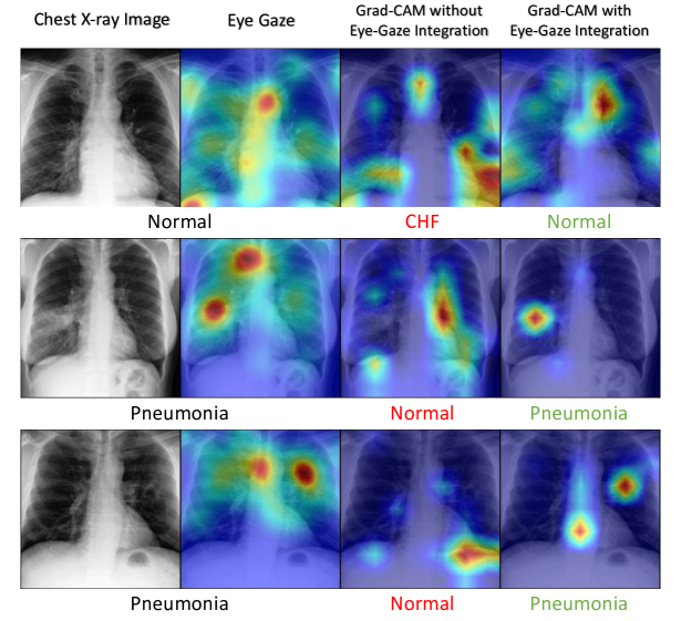
Figure 5: Gaze map and Grad-CAM based attention maps with and without eye-gaze data are shown. Under the images, original label of the chest X-ray is represented by the black color, while the red and green labels indicate incorrect and correct model predictions, respectively.

To study the effectiveness of the gaze information, we remove the gaze embedding and only fuse the features from patch embedding and position embedding. In this way, gaze information is not used. The comparison is presented in Table 5 and supplementary. Without the gaze information, accuracy, average AUC, precision, recall, and F1-score all descend. This validates the assumption that introducing the eye-gaze data can improve classification performance. It is noted that even without gaze embedding, our obtained accuracy is higher than 80% and the average AUC is higher than 0.900, superior to most gaze-guided state-of-the-art methods. This is because the proposed graph representation is powerful enough to help the model recognize the image.

Table 5: Ablation study on GazeGNN with/without the eye-gaze information.

Gaze	Accuracy	Average AUC	Precision	Recall	F1-Score
✓	83.18%	0.923	0.839	0.821	0.823
2717	80.37%	0.910	0.800	0.805	0.801

In addition, we visualize the model’s intermediate features to show the power of eye-gaze integration. We use Grad-CAM [34] to generate the attention map from the trained model. From Fig. 5, it is observed that before the eye-gaze integration, the model fails to focus on the abnormal regions, resulting in incorrect classification decisions. However, when eye-gaze is introduced, the model’s attention shifts to the regions highlighted by radiologists. This indicates the guidance of eye-gaze enhances the model’s capability to achieve more accurate abnormality localization.

5 Conclusion

In this study, we propose a novel gaze-guided graph neural network, GazeGNN, to perform the disease classification task. With the flexibility of graph representation, GazeGNN can utilize the raw eye-gaze information directly by embedding it with the image patch and the position information into the graph nodes. Therefore, this method avoids generating the VAMs that are required in mainstream gaze-guided methods. With this benefit, we develop a real-time, end-to-end disease classification algorithm without preparing the visual attention maps in advance. We show that GazeGNN can produce a significantly better performance than existing methods under the same training strategy. This proves the feasibility of bringing real-time eye tracking techniques to radiologists’ daily work.

6 Acknowledgment

This study is supported by NIH R01-CA246704, R01-CA240639, R15-EB030356, R03-EB032943, U01-DK127384-02S1, and U01-CA268808. Sincerely thank Mingfu Liang from Northwestern University for the constructive suggestions on this paper.

References

- [1] Ivo M Baltruschat, Hannes Nickisch, Michael Grass, Tobias Knopp, and Axel Saalbach. Comparison of deep learning approaches for multi-label chest x-ray classification. Scientific reports, 9(1):1–10, 2019.
- [2] Moinak Bhattacharya, Shubham Jain, and Prateek Prasanna. Gazeradar: A gaze and radiomics-guided disease localization framework. In Medical Image Computing and Computer Assisted Intervention–MICCAI 2022: 25th International Conference, Singapore, September 18–22, 2022, Proceedings, Part III, pages 686–696. Springer, 2022.
- [3] Moinak Bhattacharya, Shubham Jain, and Prateek Prasanna. Radiotransformer: A cascaded global-focal transformer for visual attention–guided disease classification. In Computer Vision–ECCV 2022: 17th European Conference, Tel Aviv, Israel, October 23–27, 2022, Proceedings, Part XXI, pages 679–698. Springer, 2022.
- [4] Aurelia Bustos, Antonio Pertusa, Jose-Maria Salinas, and Maria de la Iglesia-Vayá. Padchest: A large chest x-ray image dataset with multi-label annotated reports. Medical image analysis, 66:101797, 2020.
- [5] Li Sze Chow and Raveendran Paramesran. Review of medical image quality assessment. Biomedical signal processing and control, 27:145–154, 2016.
- [6] Dina Demner-Fushman, Sameer Antani, Matthew Simpson, and George R Thoma. Design and development of a multimodal biomedical information retrieval system. Journal of Computing Science and Engineering, 6(2):168–177, 2012.
- [7] Jia Deng, Wei Dong, Richard Socher, Li-Jia Li, Kai Li, and Li Fei-Fei. Imagenet: A large-scale hierarchical image database. In 2009 IEEE conference on computer vision and pattern recognition, pages 248–255. Ieee, 2009.
- [8] Yuyang Gao, Tong Steven Sun, Liang Zhao, and Sungsoo Ray Hong. Aligning eyes between humans and deep neural network through interactive attention alignment. Proceedings of the ACM on Human-Computer Interaction, 6(CSCW2):1–28, 2022.
- [9] Sebastian Guendel, Sasa Grbic, Bogdan Georgescu, Siqi Liu, Andreas Maier, and Dorin Comaniciu. Learning to recognize abnormalities in chest x-rays with location-aware dense networks. In Progress in Pattern Recognition, Image Analysis, Computer Vision, and Applications: 23rd Iberoamerican Congress, CIARP 2018, Madrid, Spain, November 19-22, 2018, Proceedings 23, pages 757–765. Springer, 2019.
- [10] Will Hamilton, Zhitao Ying, and Jure Leskovec. Inductive representation learning on large graphs. Advances in neural information processing systems, 30, 2017.
- [11] Kai Han, Yunhe Wang, Jianyuan Guo, Yehui Tang, and Enhua Wu. Vision gnn: An image is worth graph of nodes. arXiv preprint arXiv:2206.00272, 2022.
- [12] Kaiming He, Xiangyu Zhang, Shaoqing Ren, and Jian Sun. Deep residual learning for image recognition. In Proceedings of the IEEE conference on computer vision and pattern recognition, pages 770–778, 2016.
- [13] Gao Huang, Zhuang Liu, Laurens Van Der Maaten, and Kilian Q Weinberger. Densely connected convolutional networks. In Proceedings of the IEEE conference on computer vision and pattern recognition, pages 4700–4708, 2017.
- [14] Sergey Ioffe and Christian Szegedy. Batch normalization: Accelerating deep network training by reducing internal covariate shift. In International conference on machine learning, pages 448–456. pmlr, 2015.
- [15] Jeremy Irvin, Pranav Rajpurkar, Michael Ko, Yifan Yu, Silviana Ciurea-Ilcus, Chris Chute, Henrik Marklund, Behzad Haghgoo, Robyn Ball, Katie Shpanskaya, et al. Chexpert: A large chest radiograph dataset with uncertainty labels and expert comparison. In Proceedings of the AAAI conference on artificial intelligence, volume 33, pages 590–597, 2019.
- [16] Mohammad Tariqul Islam, Md Abdul Aowal, Ahmed Tahseen Minhaz, and Khalid Ashraf. Abnormality detection and localization in chest x-rays using deep convolutional neural networks. arXiv preprint arXiv:1705.09850, 2017.
- [17] Alistair EW Johnson, Tom J Pollard, Seth J Berkowitz, Nathaniel R Greenbaum, Matthew P Lungren, Chih-ying Deng, Roger G Mark, and Steven Horng. Mimic-cxr, a de-identified publicly available database of chest radiographs with free-text reports. Scientific data, 6(1):317, 2019.
- [18] Alexandros Karargyris, Satyananda Kashyap, Ismini Lourentzou, Joy T Wu, Arjun Sharma, Matthew Tong, Shafiq Abedin, David Beymer, Vandana Mukherjee, Elizabeth A Krupinski, et al. Creation and validation of a chest x-ray dataset with eye-tracking and report dictation for ai development. Scientific data, 8(1):92, 2021.
- [19] Daniel S Kermany, Michael Goldbaum, Wenjia Cai, Carolina CS Valentim, Huiying Liang, Sally L Baxter, Alex McKeown, Ge Yang, Xiaokang Wu, Fangbing Yan, et al. Identifying medical diagnoses and treatable diseases by image-based deep learning. cell, 172(5):1122–1131, 2018.
- [20] Naji Khosravan, Haydar Celik, Baris Turkbey, Ruida Cheng, Evan McCreedy, Matthew McAuliffe, Sandra Bednarova, Elizabeth Jones, Xinjian Chen, Peter Choyke, et al. Gaze2segment: a pilot study for integrating eye-tracking technology into medical image segmentation. In Medical Computer Vision and Bayesian and Graphical Models for Biomedical Imaging: MICCAI 2016 International Workshops, MCV and BAMBI, Athens, Greece, October 21, 2016, Revised Selected Papers 8, pages 94–104. Springer, 2017.
- [21] Naji Khosravan, Haydar Celik, Baris Turkbey, Elizabeth C Jones, Bradford Wood, and Ulas Bagci. A collaborative computer aided diagnosis (c-cad) system with eye-tracking, sparse attentional model, and deep learning. Medical image analysis, 51:101–115, 2019.
- [22] Alex Krizhevsky, Ilya Sutskever, and Geoffrey E Hinton. Imagenet classification with deep convolutional neural networks. Communications of the ACM, 60(6):84–90, 2017.
- [23] Yann LeCun, Léon Bottou, Yoshua Bengio, and Patrick Haffner. Gradient-based learning applied to document recognition. Proceedings of the IEEE, 86(11):2278–2324, 1998.
- [24] Guohao Li, Matthias Muller, Ali Thabet, and Bernard Ghanem. Deepgcns: Can gcns go as deep as cnns? In Proceedings of the IEEE/CVF international conference on computer vision, pages 9267–9276, 2019.
- [25] Ze Liu, Yutong Lin, Yue Cao, Han Hu, Yixuan Wei, Zheng Zhang, Stephen Lin, and Baining Guo. Swin transformer: Hierarchical vision transformer using shifted windows. In Proceedings of the IEEE/CVF international conference on computer vision, pages 10012–10022, 2021.
- [26] Ilya Loshchilov and Frank Hutter. Decoupled weight decay regularization. In International Conference on Learning Representations, 2018.
- [27] Chong Ma, Lin Zhao, Yuzhong Chen, David Weizhong Liu, Xi Jiang, Tuo Zhang, Xintao Hu, Dinggang Shen, Dajiang Zhu, and Tianming Liu. Rectify vit shortcut learning by visual saliency. arXiv preprint arXiv:2206.08567, 2022.
- [28] Chong Ma, Lin Zhao, Yuzhong Chen, Lu Zhang, Zhenxiang Xiao, Haixing Dai, David Liu, Zihao Wu, Zhengliang Liu, Sheng Wang, et al. Eye-gaze-guided vision transformer for rectifying shortcut learning. arXiv preprint arXiv:2205.12466, 2022.
- [29] MA Périard and P Chaloner. Diagnostic x-ray imaging quality assurance: an overview. Canadian Journal of Medical Radiation Technology, 27:171–177, 1996.
- [30] Pranav Rajpurkar, Jeremy Irvin, Kaylie Zhu, Brandon Yang, Hershel Mehta, Tony Duan, Daisy Ding, Aarti Bagul, Curtis Langlotz, Katie Shpanskaya, et al. Chexnet: Radiologist-level pneumonia detection on chest x-rays with deep learning. arXiv preprint arXiv:1711.05225, 2017.
- [31] Yao Rong, Wenjia Xu, Zeynep Akata, and Enkelejda Kasneci. Human attention in fine-grained classification. arXiv preprint arXiv:2111.01628, 2021.
- [32] K Rossmann and Bruce E Wiley. The central problem in the study of radiographic image quality. Radiology, 96(1):113–118, 1970.
- [33] Khaled Saab, Sarah M Hooper, Nimit S Sohoni, Jupinder Parmar, Brian Pogatchnik, Sen Wu, Jared A Dunnmon, Hongyang R Zhang, Daniel Rubin, and Christopher Ré. Observational supervision for medical image classification using gaze data. In Medical Image Computing and Computer Assisted Intervention–MICCAI 2021: 24th International Conference, Strasbourg, France, September 27–October 1, 2021, Proceedings, Part II 24, pages 603–614. Springer, 2021.
- [34] Ramprasaath R Selvaraju, Michael Cogswell, Abhishek Das, Ramakrishna Vedantam, Devi Parikh, and Dhruv Batra. Grad-cam: Visual explanations from deep networks via gradient-based localization. In Proceedings of the IEEE international conference on computer vision, pages 618–626, 2017.
- [35] Hoo-Chang Shin, Kirk Roberts, Le Lu, Dina Demner-Fushman, Jianhua Yao, and Ronald M Summers. Learning to read chest x-rays: Recurrent neural cascade model for automated image annotation. In Proceedings of the IEEE conference on computer vision and pattern recognition, pages 2497–2506, 2016.
- [36] Karen Simonyan and Andrew Zisserman. Very deep convolutional networks for large-scale image recognition. arXiv preprint arXiv:1409.1556, 2014.
- [37] Joseph N Stember, Haydar Celik, David Gutman, Nathaniel Swinburne, Robert Young, Sarah Eskreis-Winkler, Andrei Holodny, Sachin Jambawalikar, Bradford J Wood, Peter D Chang, et al. Integrating eye tracking and speech recognition accurately annotates mr brain images for deep learning: proof of principle. Radiology: Artificial Intelligence, 3(1):e200047, 2020.
- [38] Joseph N Stember, Haydar Celik, E Krupinski, Peter D Chang, Simukayi Mutasa, Bradford J Wood, A Lignelli, Gul Moonis, LH Schwartz, Sachin Jambawalikar, et al. Eye tracking for deep learning segmentation using convolutional neural networks. Journal of digital imaging, 32:597–604, 2019.
- [39] Tom van Sonsbeek, Xiantong Zhen, Dwarikanath Mahapatra, and Marcel Worring. Probabilistic integration of object level annotations in chest x-ray classification. In Proceedings of the IEEE/CVF Winter Conference on Applications of Computer Vision, pages 3630–3640, 2023.
- [40] Bin Wang, Armstrong Aboah, Zheyuan Zhang, and Ulas Bagci. Gazesam: What you see is what you segment. arXiv preprint arXiv:2304.13844, 2023.
- [41] Bin Wang, Lin Teng, Lanzhuju Mei, Zhiming Cui, Xuanang Xu, Qianjin Feng, and Dinggang Shen. Deep learning-based head and neck radiotherapy planning dose prediction via beam-wise dose decomposition. In International Conference on Medical Image Computing and Computer-Assisted Intervention, pages 575–584. Springer, 2022.
- [42] Sheng Wang, Xi Ouyang, Tianming Liu, Qian Wang, and Dinggang Shen. Follow my eye: using gaze to supervise computer-aided diagnosis. IEEE Transactions on Medical Imaging, 41(7):1688–1698, 2022.
- [43] Wenhai Wang, Enze Xie, Xiang Li, Deng-Ping Fan, Kaitao Song, Ding Liang, Tong Lu, Ping Luo, and Ling Shao. Pvt v2: Improved baselines with pyramid vision transformer. Computational Visual Media, 8(3):415–424, 2022.
- [44] Akino Watanabe, Sara Ketabi, Khashayar Namdar, and Farzad Khalvati. Improving disease classification performance and explainability of deep learning models in radiology with heatmap generators. Frontiers in Radiology, page 35, 2022.
- [45] Claire S Zhu, Paul F Pinsky, Barnett S Kramer, Philip C Prorok, Mark P Purdue, Christine D Berg, and John K Gohagan. The prostate, lung, colorectal, and ovarian cancer screening trial and its associated research resource. Journal of the National Cancer Institute, 105(22):1684–1693, 2013.
- [46] Hongzhi Zhu, Septimiu Salcudean, and Robert Rohling. Gaze-guided class activation mapping: leveraging human attention for network attention in chest x-rays classification. arXiv preprint arXiv:2202.07107, 2022.