First Light And Reionisation Epoch Simulations (FLARES) XIII: The Lyman-continuum emission of high-redshift galaxies

Abstract

The history of reionisation is highly dependent on the ionising properties of high-redshift galaxies. It is therefore important to have a solid understanding of how the ionising properties of galaxies are linked to physical and observable quantities. In this paper, we use the First Light and Reionisation Epoch Simulations (Flares) to study the Lyman-continuum (LyC, i.e. hydrogen-ionising) emission of massive ($M_{*}>10^{8}\,\mathrm{M_{\odot}}$) galaxies at redshifts $z=5-10$. We find that the specific ionising emissivity (i.e. intrinsic ionising emissivity per unit stellar mass) decreases as stellar mass increases, due to the combined effects of increasing age and metallicity. Flares predicts a median ionising photon production efficiency (i.e. intrinsic ionising emissivity per unit intrinsic far-UV luminosity) of $\log_{10}(\xi_{\rm ion}\rm{/erg^{-1}Hz})=25.40^{+0.16}_{-0.17}$, with values spanning the range $\log_{10}(\xi_{\rm ion}\rm{/erg^{-1}Hz})=25-25.75$. This is within the range of many observational estimates, but below some of the extremes observed. We compare the production efficiency with observable properties, and find a weak negative correlation with the UV-continuum slope, and a positive correlation with the [O iii] equivalent width. We also consider the dust-attenuated production efficiency (i.e. intrinsic ionising emissivity per unit dust-attenuated far-UV luminosity), and find a median of $\log_{10}(\xi_{\rm ion}\rm{/erg^{-1}Hz})\sim 25.5$. Within our sample of $M_{*}>10^{8}\,\mathrm{M_{\odot}}$ galaxies, it is the stellar populations in low mass galaxies that contribute the most to the total ionising emissivity. Active galactic nuclei (AGN) emission accounts for $10-20$% of the total emissivity at a given redshift, and extends the LyC luminosity function by $\sim 0.5$ dex.

1 Introduction

The Epoch of Reionisation (EoR) is the period of cosmic history in which hydrogen in the intergalactic medium (IGM) transitioned from a neutral to ionised state. Understanding how this process occurred is one of the key goals of modern extragalactic astrophysics. In the prevailing model, reionisation is driven by ionising radiation from stars and active galactic nuclei (AGN) (Dayal & Ferrara, 2018; Robertson, 2022), and is complete in most regions by $z=5-6$ (Fan et al., 2006; McGreer et al., 2015; Eilers et al., 2018; Yang et al., 2020; Choudhury et al., 2021; Bosman et al., 2022). Various theoretical and observational studies have shown that stars are likely the dominant source of ionising photons (Duncan & Conselice, 2015; Onoue et al., 2017; Dayal et al., 2020; Yung et al., 2021; Yeh et al., 2023). In addition, many models suggest a greater overall contribution from low-mass galaxies ($M_{\star}<10^{9}\,\rm{M_{\odot}}$), though uncertainties remain regarding the exact makeup of the ionising photon budget and how it changes with redshift (Finkelstein et al., 2019; Lewis et al., 2020; Yung et al., 2020b; Bera et al., 2022; Mutch et al., 2023).

An important parameter that describes the ionising output of a source is its escaping ionising emissivity $\dot{N}_{\rm ion,esc}$, defined as the rate at which escaping ionising photons are produced. Most ionising photons produced inside a galaxy are reprocessed by gas and dust in the interstellar medium (ISM). The escape fraction $f_{\rm esc}$ is the fraction of ionising photons that manage to escape the galactic environment. It follows that $\dot{N}_{\rm ion,esc}$ is obtained by combining $f_{\rm esc}$ with the intrinsic ionising emissivity $\dot{N}_{\rm ion,intr}$, the rate at which all ionising photons are produced, including those that end up reprocessed:

$$\dot{N}_{\rm ion,esc}=f_{\rm esc}\times\dot{N}_{\rm ion,intr}.$$ (1)

Note that $\dot{N}_{\rm ion,intr}$ is the integral over the stellar spectral energy distribution (SED) of a galaxy above the Lyman limit (912Å):

$$\dot{N}_{\rm ion,intr}=\int_{\nu_{912}}^{\infty}L_{\nu}(h\nu)^{-1}\rm{d}\nu.$$ (2)

$\dot{N}_{\rm ion,intr}$ is often quantified by the ionising photon production efficiency, $\xi_{\rm ion}$. Depending on the context, $\xi_{\rm ion}$ can be defined as a normalisation by stellar mass $M_{\star}$, or more commonly amongst observers, the intrinsic far-UV luminosity $L_{\rm FUV}$ (measured at rest-frame 1500Å). In this paper, we use the latter definition:

$$\xi_{\rm ion}=\frac{\dot{N}_{\rm ion,intr}}{L_{\rm FUV}}.$$ (3)

We refer to the former definition, i.e. $\dot{N}_{\rm ion,intr}/M_{\star}$, as the specific ionising emissivity.

The ionising photon production efficiency has been the target of a number of observational studies in recent years, and the rapidly expanding availability of observations from the James Webb Space Telescope (JWST) is now enabling more robust constraints on this key parameter at redshifts relevant to reionisation. Numbers derived are generally in the range $\log_{10}(\xi_{\rm ion}\rm{/\,erg^{-1}\,Hz})=25-26$ (e.g. Shivaei et al., 2018; Emami et al., 2020; Castellano et al., 2022), although some studies have measured larger values, with $\log_{10}(\xi_{\rm ion}\rm{/\,erg^{-1}Hz})>26$ (Endsley et al., 2021; Ning et al., 2022; Simmonds et al., 2023). The production efficiency is often inferred from stellar population synthesis (SPS) models through SED fitting (e.g. Castellano et al., 2022; Endsley et al., 2022; Tang et al., 2023), or using emission line fluxes, typically the Balmer recombination lines (e.g. Nakajima et al., 2016; Matthee et al., 2022; Fujimoto et al., 2023). In the former scenario, the intrinsic ionising emissivity $\dot{N}_{\rm ion,intr}$ is obtained from the fitted galaxy SED model, following Equation 2. In the latter scenario, $\dot{N}_{\rm ion,intr}$ can be estimated from the flux of the Balmer lines, using a conversion factor supplied by stellar evolution models (e.g. Leitherer & Heckman, 1995; Schaerer, 2003).

Theoretical studies have also played a part in developing our understanding of the production efficiency of distant galaxies. Wilkins et al. (2016) modelled the ionising photon production efficiency of galaxies in the BlueTides simulations, predicting values of $\log_{10}(\xi_{\rm ion}\rm{/\,erg^{-1}Hz})\approx 25.1-25.5$ for a range of stellar population synthesis (SPS) models. A similar spread of values was obtained by Ceverino et al. (2019), who modelled the SEDs of galaxies in the FirstLight simulations, and by Yung et al. (2020a), who used a semi-analytic modelling approach. Both Wilkins et al. (2016) and Yung et al. (2020a) showed that accounting for binary stellar populations results in production efficiencies that are higher by $\sim 0.2$ dex, and hence a better match to observed values. Binary evolution pathways are an important source of ionising photons (Ma et al., 2016; Eldridge & Stanway, 2020). Processes such as stripping, mass transfer, and mergers result in prolonged Lyman-continuum (LyC) emission compared to single star populations (Eldridge et al., 2008; Stanway et al., 2016; Götberg et al., 2019). In addition, massive stars with low metallicities undergo quasi-homogeneous evolution, in which the rotational mixing that results from mass transfer leads to higher surface temperatures – and hence stronger LyC emission (Stanway et al., 2016).

In this work, we use the First Light and Reionisation Epoch Simulations (Flares Lovell et al., 2021; Vijayan et al., 2021) to make predictions for the ionising emissivity, specific ionising emissivity, and ionising photon production efficiency of galaxies with $M_{\star}\gtrsim 10^{8}\ {\rm M_{\odot}}$ at $z=5-10$. Flares is a suite of high-redshift hydrodynamic zoom simulations, run using the Eagle subgrid physics model (Crain et al., 2015; Schaye et al., 2015). In the zoom simulation method, regions are selected from a dark matter-only (DMO) parent box and resimulated with hydrodynamics. By sampling a wide range of overdensities, and doing so with emphasis on highly overdense regions, we are able to efficiently simulate a large number of galaxies from a variety of environments. We note that in our analysis, the regions are weighted so as to recover the correct distribution of environments in the universe. This results in a galaxy sample with a wide range of properties that better represents the distribution of galaxies in our actual universe – essential for studying trends in galaxy properties, and making predictions for observations, particularly those from JWST (e.g. Lovell et al., 2022; Roper et al., 2022; Wilkins et al., 2022; Thomas et al., 2023).

The paper is structured as follows: in Section 2, we use a toy model to explore how the specific emissivity and production efficiency are affected by star formation, metal enrichment, SPS model and initial mass function (IMF). In Section 3, we introduce Flares and explain our methodology. Sections 4, 5 and 6 contain our analysis of the specific ionising emissivity, ionising photon production efficiency and ionising emissivity respectively. Finally, we summarise our findings in this work and present our conclusion in Section 7.

Throughout this work, we use the word ‘ionising’ to mean ‘hydrogen-ionising’. Unless otherwise stated, we focus on stellar emission, and leave the study of AGN emission to a separate work that will contain a more in-depth analysis of AGN in Flares (Kuusisto et al., in prep). The terms ‘emissivity’ and ‘production efficiency’ are sometimes used interchangeably with ‘ionising emissivity’ and ‘ionising photon production efficiency’, respectively.

2 Theoretical Background

In this section, we use a simple model to explore theoretical predictions for the specific ionising emissivity, i.e. the rate at which ionising photons are produced by a stellar population per unit stellar mass ($\dot{N}_{\rm ion,intr}/M_{\star}$), and the ionising photon production efficiency $\xi_{\rm ion}$. Figures 1–4 show how these two properties are impacted by star formation history (SFH), metallicity, choice of SPS model, and choice of IMF. Note that Figures 1 and 2 were made using v2.2.1 of the Binary Population And Stellar Synthesis (BPASS) SPS library (Stanway & Eldridge, 2018, the default choice in Flares).

2.1 Star formation and metal enrichment history

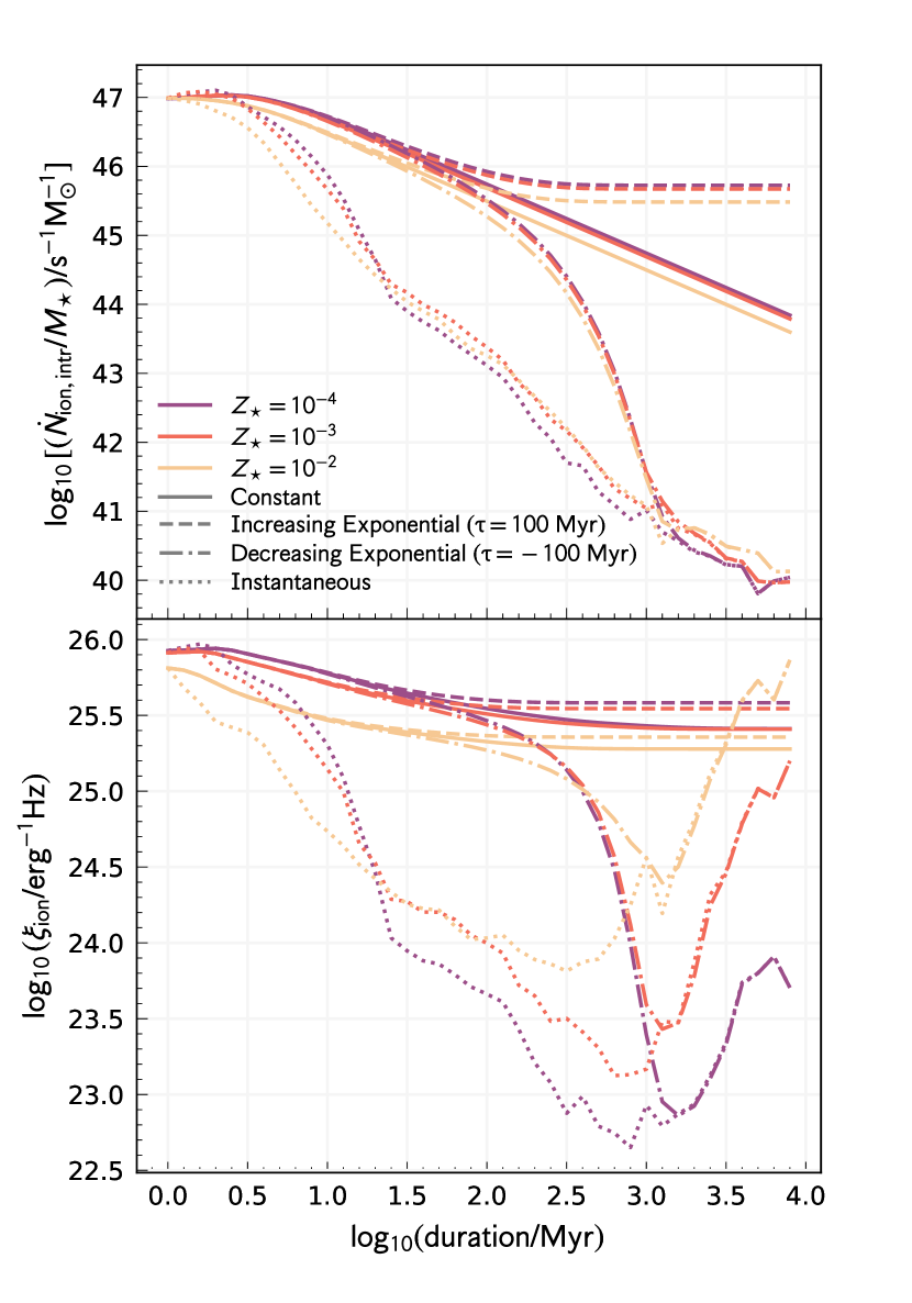
Figure 1: The specific ionising emissivity $\dot{N}_{\rm ion,intr}/M_{\star}$ (top) and production efficiency (bottom) as a function of star formation duration for a range of star formation history parameterisations and metallicities. The solid, dashed, dot-dashed, and dotted lines denote constant, increasing exponential, decreasing exponential, and an instantaneous burst of star formation, respectively.

Hot, massive stars are the main source of ionising photons in a galaxy. As these massive stars have very short lifespans, the total ionising emissivity of a stellar population declines steeply as it ages. With this in mind, we can view the specific emissivity and production efficiency as reflections of the proportion of young stars in a stellar population. Figure 1 shows how different star formation histories affect the specific emissivity and production efficiency as a function of star formation duration. Galaxies with a constant star formation history have a continuously increasing population of old stars, while young, massive stars are formed at the same rate. Hence, the proportion of young stars decreases over time in a constant star formation model, and we observe a corresponding decrease in the specific emissivity and production efficiency. In this model, the production efficiency plateaus after a certain point in time, due to the decrease in far-UV emission as stars age. For galaxies with an exponentially increasing SFH, a plateau is observed for the specific emissivity as well, as the rapidly increasing population of young stars produces enough ionising radiation to balance the increase in stellar mass. As for galaxies with an exponentially decreasing SFH, the sharp drop in the number of young stars leads to a steep drop in both the production efficiency and the specific emissivity at $\sim 10^{2.5}$ Myr. For both the decreasing exponential and instantaneous SFH, we observe an increase in the production efficiency after $\sim 1$ Gyr. This is likely due to the growing population of white dwarfs. Hot white dwarfs provide an additional source of LyC emission at late times. Due to their lower luminosity, they make a smaller contribution to the total far-UV emission than the most massive surviving Main Sequence stars, hence the increase in production efficiency. The upturn is not observed in the case of a constant or increasing SFH because the contribution of white dwarfs to the total LyC emission is relatively small. Figure 1 also shows the effect of metallicity for a given star formation history. On the whole, lower metallicities lead to higher values of the specific emissivity and production efficiency.

This is shown more clearly in Figure 2, where we plot the two properties as a function of metallicity for three different durations of continuous star formation. This reveals a strong dependence on metallicity at $Z_{\star}>0.001$, with a weaker trend at lower metallicities. From $Z_{\star}=0.001\to 0.01$, the specific emissivity and production efficiency drop by $\approx 0.2$ dex. Metals enable more efficient cooling and by the same physical process increase the opacity of stars, hence an increase in metallicity leads to stars having lower surface temperatures and consequently a lower production rate of ionising photons. The impact of different star formation durations can be attributed to varying compositions of stellar ages, as mentioned in the discussion above. A galaxy that has only been forming stars for 10 Myr would have a higher proportion of young, massive stars than a galaxy that has been forming stars for the last 100 Myr, leading to a higher specific emissivity and production efficiency.

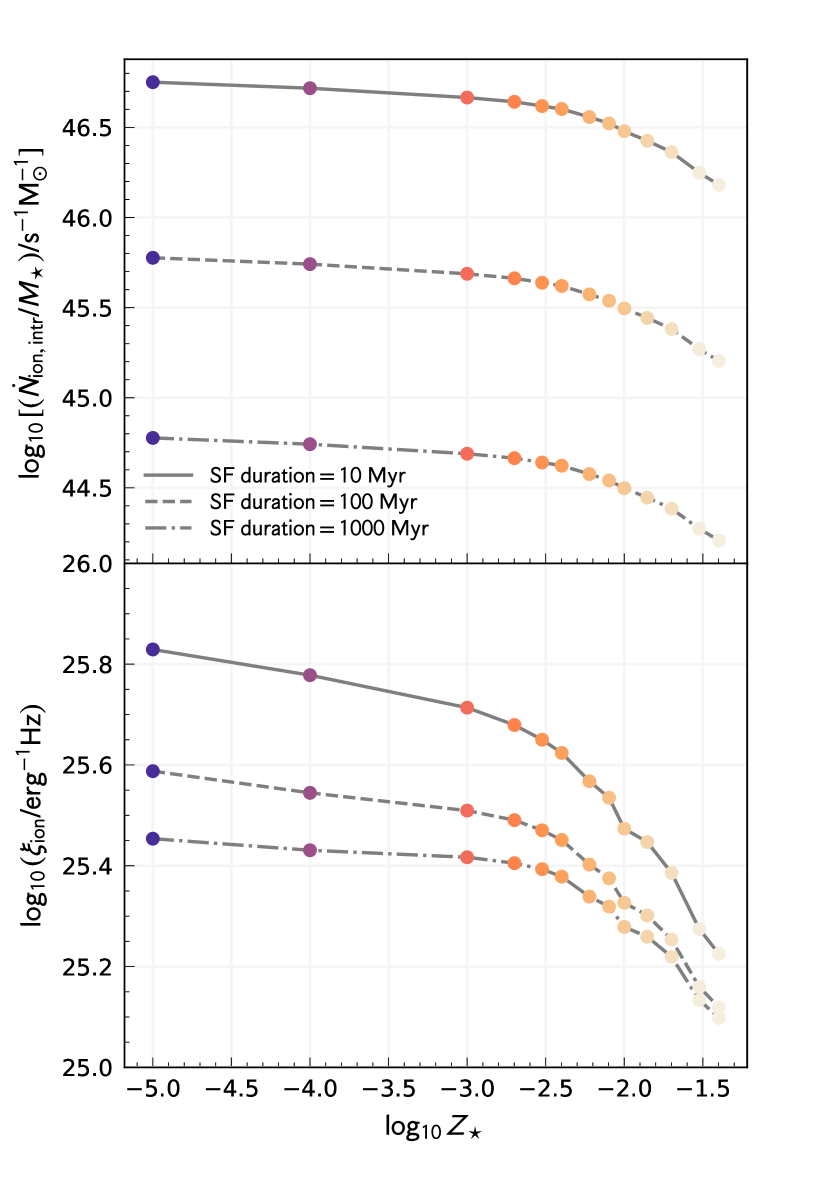
Figure 2: The specific ionising emissivity (top) and production efficiency (bottom) as a function of stellar metallicity for different star formation histories. The solid, dashed, and dot-dashed lines represent galaxies that have experienced 10, 100, and 1000 Myr of constant star formation respectively.

2.2 Choice of stellar population synthesis model

While we do not explore changing the SPS model in Flares, it is useful to consider the impact that this would have using our simple toy model. Figure 3 shows the specific emissivity and production efficiency as a function of metallicity for three different SPS models: Binary Population And Stellar Synthesis (BPASS) v2.2.1 (Stanway & Eldridge, 2018), Flexible Stellar Population Synthesis (FSPS) v3.2 (Conroy et al., 2009; Conroy & Gunn, 2010), and BC03 (Bruzual & Charlot, 2003). In each case, we assume 10 Myr constant star formation. Considering an upper-mass limit of $100\,\rm{M_{\odot}}$, we find that BPASS and FSPS yield comparable specific emissivities and production efficiencies at typical Flares metallicities (0.001-0.01). Outside of this metallicity range, using FSPS results in higher values of the production efficiency than BPASS, while BC03 consistently assigns lower values of the production efficiency except at the highest metallicities.

The effect of binaries can be seen by comparing the single-star and binary BPASS models with an upper-mass limit $m_{\rm up}=300\,\rm{M_{\odot}}$. (We note here that FLARES uses a similar binary BPASS model with $m_{\rm up}=300\,\rm{M_{\odot}}$). The inclusion of binary systems has a greater impact at lower metallicities, boosting the specific emissivity by $\sim 0.1$ dex and the production efficiency by $\sim 0.05$ dex at $Z_{\star}<10^{-2.5}$. In a similar analysis, Shivaei et al. (2018) compared binary and single-star BPASS (v2) models and found that for galaxies with 300 Myr constant star formation and a metallicity of $Z_{\star}=10^{-2.7}$, the presence of binaries increases the production efficiency by 0.17 dex.

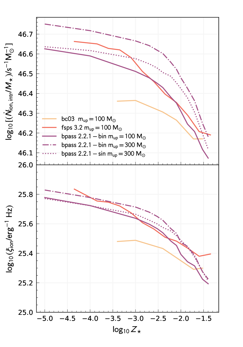
Figure 3: The specific ionising emissivity (top) and production efficiency (bottom) as a function of stellar metallicity, assuming 10 Myr of constant star formation. This is shown for different SPS models (BPASS v2.2.1, BC03, FSPS v3.2). The solid lines represent models with an upper-mass limit of 100 ${\rm M_{\odot}}$. The binary BPASS model with an upper-mass limit of 300 ${\rm M_{\odot}}$ is shown by the dot-dashed line, while the single-star BPASS model with an upper-mass limit of 300 ${\rm M_{\odot}}$ is shown by the dotted line.

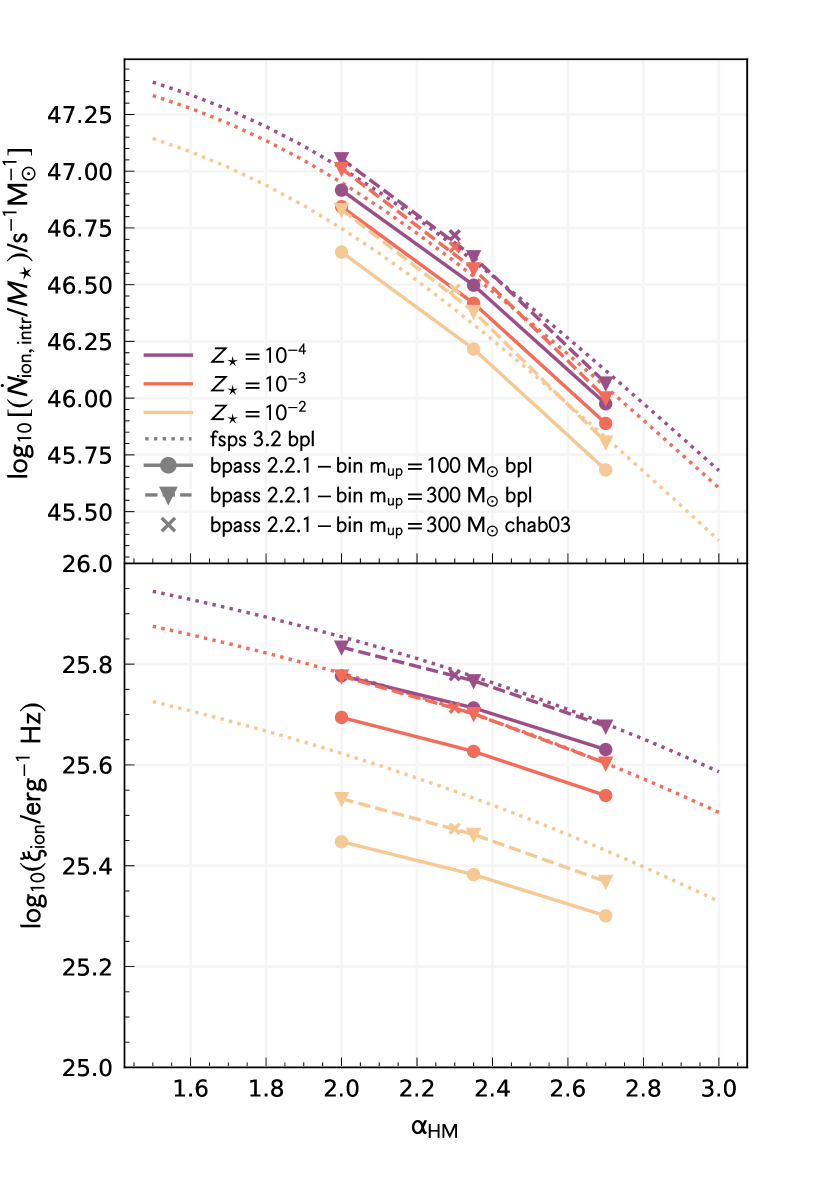
Figure 4: The specific ionising emissivity (top) and production efficiency (bottom) as a function of the high-mass slope for a range of metallicities and SPS models, using either a broken power law (BPL) or Chabrier (Chab03, Chabrier, 2003) IMF.

2.3 Initial mass function

In Figure 4, we show the specific emissivity and production efficiency as a function of the high-mass slope $\alpha_{\rm HM}$ for both FSPS and BPASS. In both models, $\alpha_{\rm HM}$ is the slope at $>1\,{\rm M_{\odot}}$. However, the models have a different behaviour at low-masses, explaining some of the offset between the two. Most of the examples in Figure 4 adopt a broken power law (BPL) IMF. We also include a binary BPASS model with a Chabrier (2003) IMF, as this is the form used in Flares. We find it gives a comparable result to the BPL BPASS model with the same upper-mass limit and $\alpha_{\rm HM}=2.35$ (see Stanway & Eldridge (2018) for more detail on the BPASS IMFs used).

Unsurprisingly, flattening the high-mass slope, and thus boosting the fraction of high-mass stars, yields higher emissivities. Flattening the slope by $\Delta\alpha_{\rm HM}=0.5$ increases the specific emissivity by 0.5 dex. Since flattening the slope also boosts the UV luminosity, the impact on the production efficiency is weaker, $\sim 0.2-0.3$ dex. For BPASS, we also consider two upper-mass limits: $m_{\rm up}=100$ and 300 ${\rm M_{\odot}}$. Extending the mass-range of stars to 300 ${\rm M_{\odot}}$ boosts the production efficiency by $\approx 0.15$ dex. A very similar result was found by Shivaei et al. (2018), who used v2 of the single-star BPASS model and found that increasing $m_{\rm up}$ from 100 to 300 ${\rm M_{\odot}}$ increased the production efficiency by 0.18 and 0.12 dex, assuming a high-mass slope of $\alpha_{\rm HM}=2.0$ and $\alpha_{\rm HM}=2.7$ respectively.

3 Methods

In this section, we introduce Flares, the suite of simulations used in this study. We define the physical properties used in this paper and describe the forward modelling procedure for obtaining galaxy SEDs from these physical properties.

3.1 First Light And Reionisation Epoch Simulations

The First Light And Reionisation Epoch Simulations (Flares) is a suite of hydrodynamical zoom simulations that probes galaxy formation and evolution at high redshift (Lovell et al., 2021; Vijayan et al., 2021). It consists of 40 spherical resimulations, each with a radius of 14$h^{-1}$Mpc. The regions for resimulation are selected from a (3.2 cGpc)³ parent dark matter-only (DMO) simulation, the same as that used in the C-Eagle zoom simulations (Barnes et al., 2017a). The large volume of the parent box provides access to a wide variety of environments. Taking advantage of this, the resimulated regions in Flares span an overdensity range of $\delta=-0.497\rightarrow 0.970$ (see Table A1 of Lovell et al., 2021), with a bias towards highly overdense environments, where massive galaxies are more likely to form (Chiang et al., 2013; Lovell et al., 2018). The regions are selected at $z=4.67$, when the most extreme overdensities are only mildly non-linear, so as to preserve the rank ordering of the overdensities at high redshift. When studying galaxy population statistics, it is necessary to recreate the original distribution of environments in the parent simulation. To do so, we use a weighting scheme that reduces the contribution from rarer regions, i.e. the most underdense and overdense ones (see Lovell et al. (2021) for a more detailed explanation). Throughout this work, aggregate values such as the median are obtained by applying this weighting scheme.

The Flares regions are resimulated with hydrodynamics using the AGNdT9 variant of the Eagle subgrid physics model (Schaye et al., 2015; Crain et al., 2015). The AGNdT9 variant was chosen as it produces similar mass functions as the fiducial model, while providing a better match to observations of the hot gas properties in groups and clusters (Barnes et al., 2017b). Flares has an identical resolution to the fiducial Eagle model: dark matter and initial gas particles are of mass m${}_{\mathrm{dm}}=9.7\times 10^{6}$ M_⊙ and m${}_{\mathrm{g}}=1.8\times 10^{6}$ M_⊙ respectively, with a softening length of $2.66\,\mathrm{ckpc}$. The output of the simulations is stored at integer redshifts at $z=5-15$.

3.2 Measuring galaxy properties

As with the Eagle simulation, galaxies in Flares are first grouped using the Friends-Of-Friends (FOF) algorithm (Davis et al., 1985) before being identified as substructures using the Subfind algorithm (Springel et al., 2001). All galaxy properties in this paper are measured using particles that lie within a 30 pkpc (physical kpc) aperture of the most bound particle in each substructure.

We define the age of a galaxy as the initial mass-weighted median age of its constituent stellar particles (i.e. within the 30 pkpc aperture). Metallicity is similarly defined as the initial mass-weighted median metallicity of a galaxy’s stellar particles. The star formation rate (SFR) is calculated by considering the total stellar mass formed over the most recent 50 Myr, and the specific star formation rate (sSFR) is the star formation rate per unit stellar mass.

When studying the physical properties of galaxies, we limit our analysis to galaxies with a stellar mass of $M_{*}>10^{8}\,\mathrm{M_{\odot}}$, as this is the mass range resolved by Flares. When considering the observational properties of galaxies, we add an additional cut in the dust-attenuated far-UV luminosity: $L_{\rm FUV,\,dust}>10^{28}\,\mathrm{erg\,s^{-1}\,Hz^{-1}}$ (this corresponds to a cut at $M_{\rm FUV}=-18.4$).

3.3 SED Modelling

Here we provide a brief description of the stellar SED modelling in Flares, and refer the reader to Vijayan et al. (2021) for a more in-depth explanation. The SED modelling procedure for AGN is detailed in Kuusisto et al. (in prep).

3.3.1 Stellar SED

To begin, we assign a stellar SED to each stellar particle, according to its mass, age and metallicity. We use v2.2.1 of the Binary Population And Spectral Synthesis (BPASS, Stanway & Eldridge, 2018) SPS library, and assume a Chabrier (2003) IMF. As discussed in Section 2, the SPS model and IMF used have a strong influence on the ionising properties of galaxies.

The intrinsic emissivity $\dot{N}_{\rm ion,intr}$ and intrinsic $L_{\rm UV}$ used to derive $\xi_{\rm ion}$ in Equation 3 are both obtained from pure stellar SEDs.

3.3.2 Nebular emission

Nebular emission occurs when LyC radiation from stars is reprocessed by gas and dust. We model birth clouds by associating each young stellar particle ($<10$ Myr, assuming birth clouds disperse on these timescales; Charlot & Fall, 2000) with an ionisation-bounded $\rm H_{II}$ region. Nebular emission lines are obtained by using the SED of the stellar particle as the incident radiation field in version 17.03 of the cloudy photoionisation code (Ferland et al., 2017). We assume a solar abundance pattern, a covering fraction of 1 (equivalent to $f_{\rm esc}=0$), a birth cloud metallicity identical to that of the stellar particle, and a hydrogen density of ${\rm log}_{10}(n_{\rm H}/{\rm cm}^{-3})=2.5$. Dust depletion factors and relative abundances are taken from Gutkin et al. (2016). We use a metallicity- and age- dependent ionisation parameter $U$, scaled from a reference value of $U_{\rm ref}=10^{-2}$ at $Z_{\rm\star,ref}=0.02$ and $t_{\rm ref}=1$ Myr. For a spherical ionised region around a stellar particle of metallicity $Z_{\star}$ and age $t$, $U$ scales with the intrinsic ionising emissivity $\dot{N}_{\rm ion}$ of the stellar particle as follows:

$$U(Z_{\star},t)=U_{\rm ref}\left(\frac{\dot{N}_{\rm ion}(Z_{\star},t)}{\dot{N}_{\rm ion,ref}(Z_{\rm\star,ref},t_{\rm ref})}\right)^{1/3}.$$ (4)

$\dot{N}_{\rm ion,ref}$ is the reference emissivity, obtained for a stellar particle with metallicity $Z_{\rm\star,ref}$ and age $t_{\rm ref}$. We refer the interested reader to Section 2.1.2 of Wilkins et al. (2023a) for a more comprehensive explanation.

3.3.3 Dust attenuation

There are two components to our dust model: the first accounts for dust extinction in the birth cloud, and the second accounts for dust extinction in the intervening ISM.

As with modelling nebular emission, we associate young stellar particles ($<10$ Myr) with a birth cloud. The birth cloud dust optical depth in the V-band, $\tau_{\rm BC,V}$, is taken to be metallicity-dependent:

$$\tau_{\rm BC,V}=\kappa_{\rm BC}(Z_{\star}/0.01),$$ (5)

where $Z_{\star}$ is the metallicity of the stellar particle, and $\kappa_{\rm BC}$ is a normalisation factor with a value of $1$. For older stellar particles ($>10$ Myr), $\tau_{\rm BC,V}=0$.

To model dust extinction in the intervening ISM, we treat each stellar particle as a point-like particle and take our line of sight (LOS) to be the $z$-axis. We first obtain the LOS metal column density $\Sigma(x,y)$ by integrating the density field of gas particles along the LOS, using the smoothed particle hydrodynamics (SPH) smoothing kernel of the gas particles. The column density is then converted to the ISM dust optical depth in the V-band:

$$\tau_{\rm ISM,V}(x,y)={\rm DTM}\;\kappa_{\rm ISM}\;\Sigma(x,y),$$ (6)

where DTM is the dust-to-metal ratio, obtained for each galaxy using a fitting function dependent on stellar age and gas-phase metallicity (Equation 15 in Vijayan et al., 2019). $\kappa_{\rm ISM}$ is a normalisation factor with a value of 0.0795, chosen to match the $z=5$ UV luminosity function in Bouwens et al. (2015).

The optical depth at other wavelengths is given by an inverse power law:

$$\tau_{\lambda}=(\tau_{\rm BC,V}+\tau_{\rm ISM,V}(x,y))\times(\lambda/550{\rm nm})^{-1}.$$ (7)

This expression can then be applied to the stellar particle SEDs. Comparing our model with the Small Magellanic Cloud (SMC) (Pei, 1992) and Calzetti (Calzetti et al., 2000) curves, we find that the dust model detailed here results in very similar values of attenuation in the far-UV. However, measurements of the UV-continuum slope $\beta$ are more sensitive to the choice of attenuation curve. The Flares dust model is flatter in the UV than the SMC curve, though not as much as the Calzetti curve, leading to values of $\beta$ in between the two curves, but closer to the SMC values (see Section C1 of the Appendix in Vijayan et al., 2021).

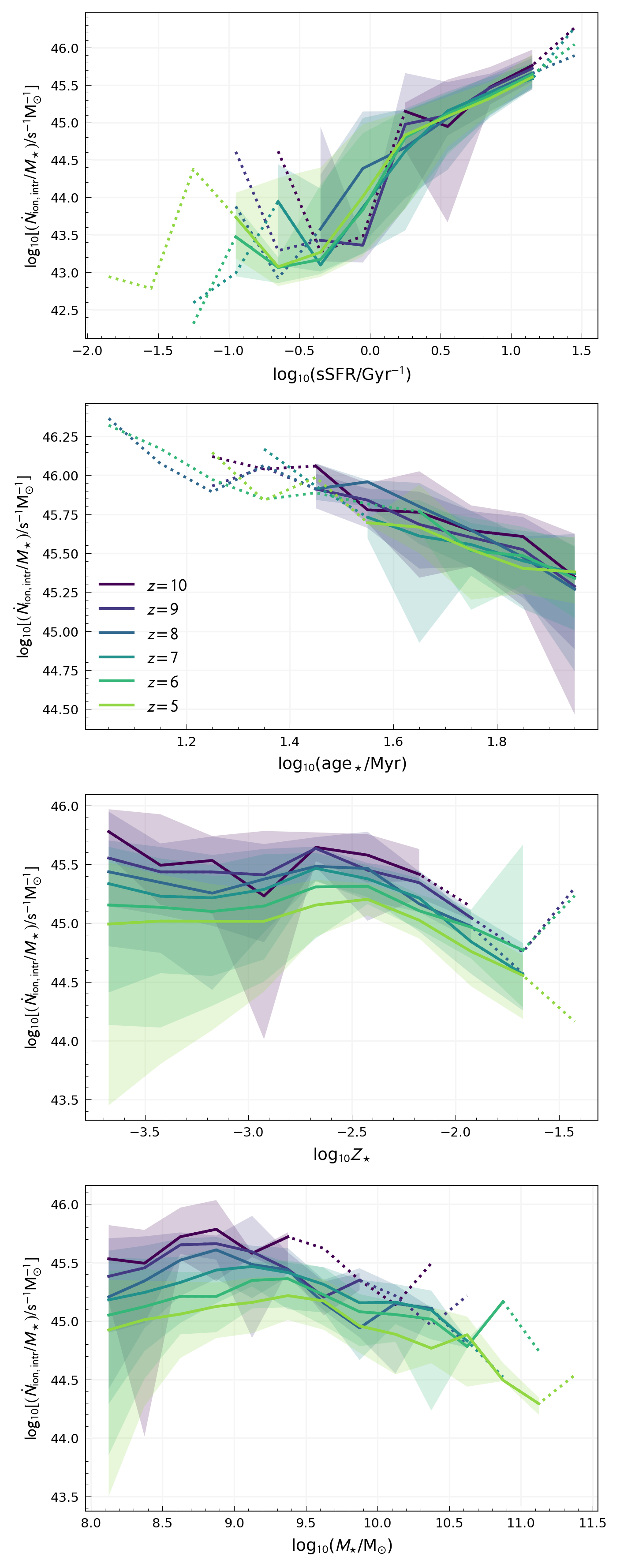
Figure 5: Specific ionising emissivity as a function of (from top to bottom): specific star formation rate, stellar age, stellar metallicity, and stellar mass. Trend lines show the weighted median specific ionising emissivity, and are coloured by redshift. Dotted lines are used to represent bins containing fewer than 10 galaxies. Shaded regions denote the 16-84th percentile range.

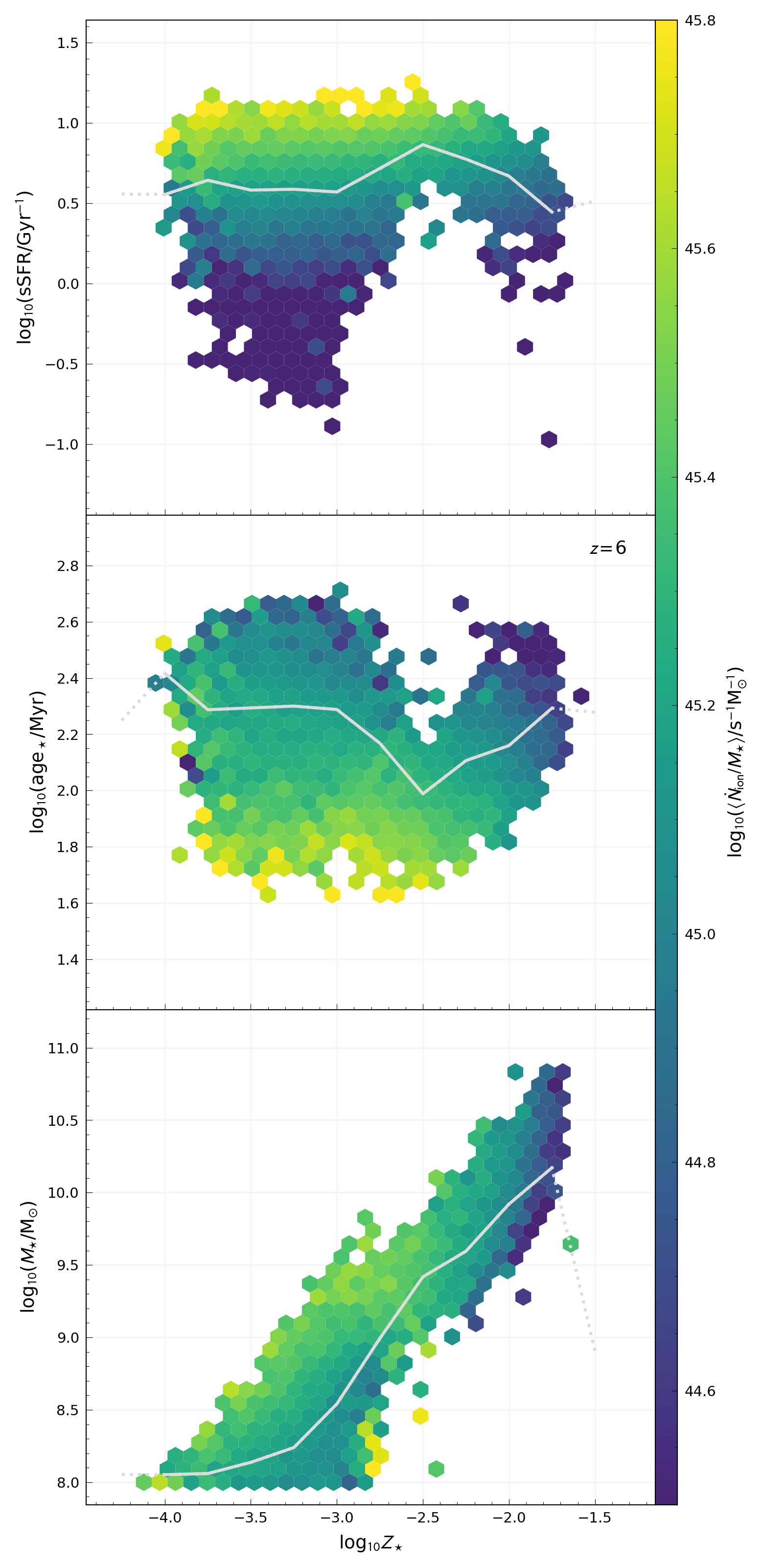
Figure 6: (From top to bottom) Stellar age, specific star formation rate and stellar mass as a function of stellar metallicity at $z=6$. Similar trends are observed at other redshifts. The hex bins are coloured by mean specific ionising emissivity (only bins containing two or more galaxies are displayed). The weighted median line in grey accounts for all galaxies, including those not displayed in a hex bin.

4 Specific ionising emissivity

In this section, we study the dependence of the specific ionising emissivity, defined as the intrinsic ionising emissivity per unit stellar mass ($\dot{N}_{\rm ion,intr}/M_{\star}$), on the following physical properties: specific star formation rate, age, metallicity, and stellar mass. Wilkins et al. (2023b) have studied the star formation and metal enrichment histories of galaxies in Flares in depth. Here, we link these quantities to the specific emissivity. We focus our analysis on galaxies with $M_{\star}>10^{8}\ {\rm M_{\odot}}$.

4.1 Star formation and metal enrichment history

The first panel of Figure 5 shows a strong positive correlation between specific emissivity and specific star formation rate. As mentioned in Section 2.1, it is the young, massive, short-lived stars that produce large amounts of ionising radiation. A high specific star formation rate is indicative of a large fraction of these young stars. As such, the ionising emissivity of a galaxy essentially traces recent star formation. A tighter relation would be observed if we were to use a star formation rate defined on a shorter timescale, due to SFH variability.

The negative correlation of specific emissivity with age (second panel of Figure 5) can be explained along similar lines. Since we define age as the initial mass-weighted median age of the stellar population, the age of a galaxy tells us if its stellar population is generally young or old. The younger the stellar population, the more efficient a galaxy is at producing ionising radiation per unit mass. The effect of age is also reflected in the redshift dependence of the specific emissivity, most obvious in the third and fourth panels of Figure 5, where we see smaller values of the specific emissivity at lower redshifts, for a given metallicity or stellar mass. In the case of stellar mass, the specific emissivity decreases by $\sim 0.1$ dex between integer redshifts.

The relationship between specific emissivity and metallicity is shown in the third panel of Figure 5. At extremely low metallicities, up until $Z_{\star}\sim 10^{-3}$, the trend is more or less flat, with at most a weak relationship of decreasing specific emissivity with increasing metallicity. Past $Z_{\star}\sim 10^{-3}$, the specific emissivity increases and peaks at $Z_{\star}\sim 10^{-2.5}$, before decreasing steeply. In the top panel of Figure 2, which shows how the specific emissivity evolves with metallicity for a simple model, we see a similar distinction between trends at high and low metallicity. However, the peak is not observed in Figure 2, as it results from the more complex stellar populations of galaxies in Flares. Roper et al. (2023) investigated the size evolution of galaxies in Flares and found that galaxies around a stellar mass of $M_{\star}\sim 10^{9.5}\,\rm{M_{\odot}}$ tend to undergo a burst of star formation in their cores, triggered by enriched gas cooling to higher densities. This leads to an increased specific star formation rate – which in turn causes the specific emissivity to increase. Since galaxies in Flares exhibit a strong mass-metallicity relation (see bottom panel of Figure 6 for an example at $z=6$), we find that the burst of star formation occurs around a particular metallicity range as well. The turnover in the specific emissivity likely occurs for a few different reasons. The top panel of Figure 2 shows that the specific emissivity of a stellar population decreases more steeply at $Z_{\star}>10^{-2.5}$, as higher metallicities lead to cooler stars. There is also the role of feedback in regulating star formation – these metal-rich galaxies tend to be more massive, and likely have their star formation regulated by AGN feedback. Figure 6 presents the distribution of the physical properties of Flares galaxies at $z=6$, coloured by specific emissivity. We note that the dip in age and the peak in specific star formation rate observed at $Z_{\star}\sim 10^{-2.5}$ are associated with the aforementioned burst of star formation.

The top and middle panels of Figure 6 show how the specific emissivity is largely dictated by specific star formation rate and age. The effect of metallicity is more subtle, only becoming evident at higher metallicities ($Z_{\star}>10^{-2.5}$), where we see a slight decrease in the specific emissivity for constant values of age or specific star formation rate.

4.2 Stellar mass

In the lowermost panel of Figure 5, we observe a general trend of decreasing specific emissivity at high stellar masses ($M_{\star}>10^{9}\;\rm{M_{\odot}}$). This is primarily due to the effect of metallicity – galaxies in Flares exhibit a strong mass-metallicity relation, as shown in the bottom panel of Figure 6 (for other redshifts, see Figure 2 of Vijayan et al., 2021). The median age of galaxies is also seen to increase slightly at high stellar masses (Figure 5 of Wilkins et al., 2023b), which would also contribute to the trend. At lower stellar masses, the trend is flatter, with a tentative negative slope.

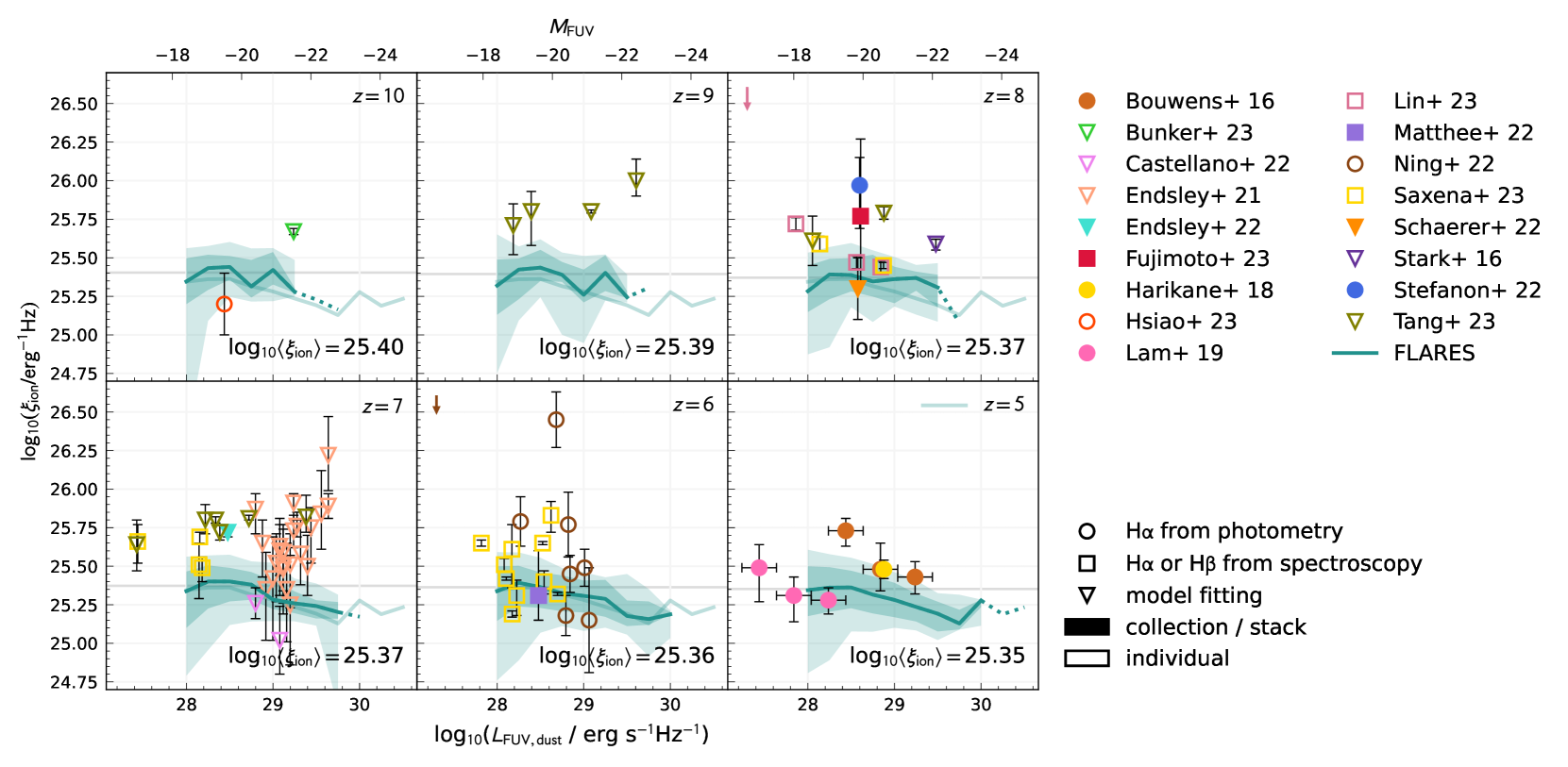
Figure 7: Ionising photon production efficiency as a function of the dust-attenuated far-UV luminosity (rest frame 1500Å), for redshifts $z=5-10$. Trend lines show the weighted median ionising photon production efficiency in Flares, and shaded regions denote the 1 and 2$\sigma$ range. The faint, horizontal grey line indicates the weighted mean of the sample at each redshift. The translucent blue line plotted across all panels shows the weighted median at $z=5$. Observations are displayed as scatter points: those with a transparent fill are measurements of individual galaxies; those with a solid fill are aggregated values, representing either stacks or collections of galaxies; circular and square data points represent measurements of the production efficiency obtained using Balmer emission line fluxes from photometry and spectroscopy respectively; triangular data points represent measurements of the production efficiency obtained from model fitting (this is a broad term that encompasses SED fitting). Observations are plotted in the panel corresponding to the nearest integer redshift. Arrows indicate how values may change when accounting for dust (for measurements by Ning et al., 2022; Lin et al., 2023). A version of this plot with $\xi_{\rm ion}$ as a function of stellar mass can be found in the Appendix (Figure 15).

5 Ionising photon production efficiency

In this section, we explore how the ionising photon production efficiency varies with observable properties, namely the far-UV luminosity, UV continuum slope and [O iii] equivalent width. Since we are now making predictions in the observer space, on top of our mass cut we impose a luminosity cut using the dust-attenuated far-UV luminosity: $\log_{10}(L_{\rm FUV,dust}/\mathrm{erg\,s^{-1}Hz^{-1}})>28$ (this corresponds to a cut at $M_{\rm FUV}=-18.4$).

For most of this section, we define the production efficiency following Equation 3, using the intrinsic far-UV luminosity to normalise the ionising emissivity. In Section 5.5, we will discuss an alternate definition of the production efficiency, $\xi_{\rm ion,dust}$, that uses the dust-attenuated far-UV luminosity in place of the intrinsic value.

We note that estimating the production efficiency from line fluxes requires an assumption of the ionising photon escape fraction $f_{\rm esc}$, as only reprocessed photons are responsible for nebular emission. For example, in the case of H$\alpha$, the intrinsic line luminosity can be expressed as (Leitherer & Heckman, 1995):

$$L_{\rm{H}\alpha}\rm{[erg\,s^{-1}]}=1.36\times 10^{-12}(1-f_{\rm{esc}})\dot{N}_{\rm ion,intr}\rm{[s^{-1}]}.$$ (8)

H$\beta$ and H$\gamma$ fluxes can be used to obtain the intrinsic ionising emissivity $\dot{N}_{\rm ion,intr}$ in the same manner, applying the appropriate conversion factors. With $f_{\rm esc}$ being a highly uncertain parameter, we choose, where possible, to compare our results with measurements that assume $f_{\rm esc}=0$, essentially considering the lower bound of the production efficiency.

5.1 High-z observations

Below, we list the high-redshift ($z>5$) observations of the production efficiency that we compare our results with (in Figures 7, 8, 9, 11 and 15). We have restricted our analysis to redshifts $z\gtrsim 5$, as this is the range targeted by Flares:

• Bouwens et al. (2016) measured $\xi_{\rm ion}$ for a sample of 22 galaxies at $z=5.1-5.4$, using H$\alpha$ fluxes estimated from SPITZER/IRAC photometry. For the values plotted, the apparent H$\alpha$ fluxes and UV-continuum were corrected for dust using measurements of the UV-continuum slope, assuming an SMC dust law (Pei, 1992). In Figure 7 (15), the galaxies are binned by luminosity (stellar mass), with bin widths denoted by error bars.

• Bunker et al. (2023) analysed JWST/NIRSpec spectroscopy of GN-z11, a Lyman break galaxy with a derived redshift of $z=10.6$. Use of the Balmer lines and SED fitting with Beagle both lead to an estimate of $\log_{10}(\xi_{\rm ion}\rm{/erg^{-1}Hz})\approx 25.7$. The calculation involving the Balmer lines does not include a dust correction, since the data suggests very little dust attenuation.

• Castellano et al. (2022) analysed VLT/X-SHOOTER observations of two $z\approx 7$ Ly$\alpha$ emitters (LAEs), thought to reside in a reionised bubble in the Bremer Deep Field (BDF). $\xi_{\rm ion}$ was obtained from a Beagle (Chevallard & Charlot, 2016) fit to the spectroscopy and available photometry in the field, assuming an exponentially delayed SFH with a 10 Myr burst of constant star formation, and dust treatment following Charlot & Fall (2000) and Chevallard et al. (2013).

• De Barros et al. (2019) analysed the Spitzer and HST photometry of $z\sim 8$ galaxies and obtained median values of $\log_{10}(\xi_{\rm ion,dust}\rm{/erg^{-1}Hz})=26.07$ and 26.29 using SMC and Calzetti dust attenuation curves, respectively. Due to uncertain parameters in the SED fitting, the authors emphasise a lower limit of $\log_{10}(\xi_{\rm ion,dust}\rm{/erg^{-1}Hz})>25.77$ (indicated by an upwards arrow in Figures 8 and 15), and note that the intrinsic $\xi_{\rm ion}$ should be very similar to $\xi_{\rm ion,dust}$, due to small dust attenuation.

• Endsley et al. (2021) studied 22 [O iii]$+\rm{H}\beta$ emitters at $z\sim 7$ and obtained $\xi_{\rm ion}$ by fitting to SPITZER/IRAC photometry with the Beagle SED fitting tool, assuming an exponentially delayed SFH with an allowed recent ($<10$ Myr) burst, and an SMC dust law.

• Endsley et al. (2022) investigated 118 Lyman-break galaxies in the Extended Goth Strip (EGS) field. $\xi_{\rm ion}$ was obtained from a Beagle fit to JWST/NIRCam and HST/ACS photometry, assuming a constant star formation history (CSFH) and an SMC dust law. The authors find evidence for high specific star formation rates, in line with the high values of $\xi_{\rm ion}$ measured.

• Faisst et al. (2019) measure $\xi_{\rm ion}$ for a collection of 221 galaxies at $z\sim 4.5$, using the H$\alpha$ line to obtain $\dot{N}_{\rm ion}$. The H$\alpha$ fluxes are estimated by comparing the measured Spitzer photometry to modelled colours from a variety of BC03 templates, focusing only on the optical continuum. We note that the calculation of $\xi_{\rm ion}$ assumes $f_{\rm esc}\sim 0.1$. A wide range of values is obtained, between $\log_{10}(\xi_{\rm ion}\rm{/erg^{-1}Hz})=24.5-26.4$ (error bars in Figure 8 show the 16th and 84th percentile values).

• Fujimoto et al. (2023) obtained $\xi_{\rm ion}$ for 7 $z\sim 8-9$ galaxies with redshifts spectroscopically confirmed using JWST/NIRSpec spectroscopy. $\xi_{\rm ion}$ was measured using the H$\beta$ line, with dust extinction obtained from a fit to HST$+$JWST/NIRCam photometry and the [O iii]$\lambda$5008 EW. The SED fitting was performed using Cigale, and assumed a delayed and final burst ($<$10 Myr) SFH, a Calzetti dust law for the stellar continuum and an SMC dust law for nebular emission.

• Harikane et al. (2018) measured $\xi_{\rm ion}$ for a stack of LAEs at $z=4.9$ (we have plotted the sample of 99 galaxies with $20<$Ly$\alpha$ EW$<100$). To infer the H$\alpha$ flux, the authors compared the stacked SED with a model SED, which was obtained from a Beagle fit assuming a CSFH and Calzetti dust curve. Taking into account the inferred escape fraction ($f_{\rm esc}=0.1$) of the sample would increase the production efficiency slightly, by $\sim 0.05$ dex.

• Hsiao et al. (2023) studied JWST/NIRSpec spectroscopy of a $z\sim 10.17$ galaxy (MACS0647-JD). $\xi_{\rm ion}$ was obtained using the H$\alpha$ flux, which was estimated from the H$\gamma$ emission line. The emission line flux and far-UV luminosity were not corrected for dust, however, results from SED fitting suggest little dust attenuation.

• Lam et al. (2019) measured $\xi_{\rm ion}$ for binned stacks of faint galaxies at $z\approx 4-5$, using imaging data from HST and SPITZER/IRAC. The H$\alpha$ flux used to calculate $\xi_{\rm ion}$ was obtained by fitting a model spectrum to the measured colours, and correcting for dust using an SMC dust law. The values plotted in Figure 7 are binned by luminosity, with bin widths denoted by error bars.

• Lin et al. (2023) analysed the JWST/NIRSpec spectra of 3 lensed $z\sim 8$ galaxies. We note that this work defined the production efficiency using the dust-attenuated H$\beta$ flux and the dust-attenuated far-UV luminosity. The arrows in Figures 7 and 8 roughly show how dust-attenuation, measured with the UV-continuum slope assuming an SMC dust law, would impact the production efficiencies ($\lesssim 0.13$ dex lower).

• Matthee et al. (2022) analysed a sample of $117$ [O iii] emitters that were observed using JWST/NIRCam wide-field slitless spectroscopy. $\xi_{\rm ion}$ was obtained using the H$\beta$ line, with dust extinction inferred from the H$\gamma/$H$\beta$ ratio.

• Ning et al. (2022) used the H$\alpha$ flux, estimated from JWST/NIRCam data, to measure $\xi_{\rm ion}$ for 7 spectroscopically confirmed Lyman break galaxies (LBGs) at $z\sim 6$. We note that this work defined the production efficiency using the dust-attenuated H$\alpha$ flux and the dust-attenuated far-UV luminosity. The arrows in Figures 7, 8 and 9 roughly show how corrections for dust would impact the production efficiencies ($\lesssim 0.1$ dex lower).

• Prieto-Lyon et al. (2023) studied a sample of $\sim 100$ $z=3-7$ galaxies using HST and JWST/NIRCam photometry. The H$\alpha$ flux was measured by comparing the observed photometry to the continuum flux, which was obtained from SED fitting using BAGPIPES, employing BC03 templates, an SMC dust law, and an exponentially rising delayed SFH. A wide range of values is obtained for the H$\alpha$ flux, and this is reflected in wide range of $\xi_{\rm ion}$ values obtained.

• Saxena et al. (2023) studied 16 faint LAEs using spectroscopic data from the JWST Advanced Deep Extragalactic Survey (JADES). The H$\alpha$ flux was used to estimate $\xi_{\rm ion}$ for all galaxies except one for which the H$\alpha$ line was not within the spectral coverage. Dust was corrected using the H$\alpha$$/$H$\beta$ ratio (H$\gamma/$H$\beta$ for the aforementioned exception).

• Schaerer et al. (2022) measured the [O iii]$\lambda$5007 EW of 3 $z\sim 8$ galaxies in the SMACS field using JWST/NIRSpec. Using relations between $\xi_{\rm ion}$ and [O iii]$\lambda$5007 at low-$z$, the authors obtained a rough estimate of $\log_{10}(\xi_{\rm ion}\rm{/erg^{-1}Hz})\approx 25.1-25.5$. In Figure 7, we have plotted a representative data point at the midpoint of this estimate and the mean far-UV luminosity of the 3 galaxies.

• Simmonds et al. (2023) obtained both $\xi_{\rm ion}$ and $\xi_{\rm ion,dust}$ for 30 $z\sim 5.4-6.6$ galaxies, using the flux excess from JWST Extragalactic Medium-band Survey (JEMS, Williams et al., 2023) observations to estimate the H$\alpha$ flux. We note that most galaxies in the sample have low values of dust attenuation and hence the values of $\xi_{\rm ion}$ and $\xi_{\rm ion,dust}$ are very similar in most cases, with a difference of at most $\sim 0.1$ dex. In Figures 8 and 9, we have plotted $\xi_{\rm ion,dust}$ and indicated with an arrow the possible range of values, should dust-attenuation be accounted for.

• Stark et al. (2015) found evidence for the CIV$\lambda$1548 line in the KECK/MOSFire observation of a gravitationally-lensed $z=7.045$ galaxy (A1703-zd6). We note that the authors use the dust-attenuated far-UV luminosity to calculate the production efficiency, i.e. they measure $\xi_{\rm ion,dust}$. The estimate for $\xi_{\rm ion,dust}$ was found by fitting the line emission and photometry to a grid of photoionisation models, generated with BC03 (Bruzual & Charlot, 2003) spectra.

• Stark et al. (2017) studied the Keck/MOSFire spectroscopy of 3 galaxies, chosen for their strong [O iii]$+\rm{H}\beta$ emission. $\xi_{\rm ion}$ was obtained from a fit to emission line and photometric constraints, using Beagle, and assuming an exponentially delayed SFH superposed with a 10 Myr burst of constant star formation. In Figure 7, we plot the galaxy EGS-zs8-1, and in Figure 8 we plot all 3 galaxies.

• Stefanon et al. (2022) stacked the SPITZER/IRAC photometry of $\sim 100$ LBGs at $z\sim 8$, and obtained $\xi_{\rm ion}$ by estimating the H$\alpha$ flux from the photometry and assuming negligible dust attenuation.

• Sun et al. (2022) measured $\xi_{\rm ion}$ for 3 H$\alpha$ $+$ [O iii]$\lambda 5007$ emitters, detected with JWST/NIRCam wide-field slitless spectroscopy (WFSS). $\dot{N}_{\rm ion}$ was obtained from the H$\alpha$ line and the far-UV luminosity from SED fitting with Cigale, assuming an exponentially delayed SFH with an optional late starburst, and a Calzetti dust law.

• Tang et al. (2023) measured $\xi_{\rm ion}$ for 12 $z>7$ galaxies from their CEERS JWST/NIRSpec sample. $\xi_{\rm ion}$ is obtained by fitting to spectroscopic data and additional photometry using Beagle, assuming a CSFH and an SMC attenutation curve.

• Whitler et al. (2023) used JWST/NIRCam data to study a sample of 28 galaxies at $z\sim 8.4-9.1$, in the vicinity of two luminous LAEs in the EGS field (the sample includes one of the luminous LAEs). $\xi_{\rm ion}$ was obtained by SED fitting with the Beagle tool, assuming a CSFH and an SMC dust law.

5.2 Far-UV luminosity

Figure 7 shows predictions for the production efficiency alongside a number of observations. For the galaxy population in Flares at $z=5-10$ with $M_{\star}>10^{8}\;\rm{M_{\odot}}$ and above the dust-attenuated luminosity threshold $\log_{10}(L_{\rm FUV,dust}/\mathrm{erg\,s^{-1}Hz^{-1}})=28$, we obtain a median production efficiency of $\log_{10}(\xi_{\rm ion}\rm{/erg^{-1}Hz})=25.40^{+0.16}_{-0.17}$, and a 2$\sigma$ range of $\log_{10}(\xi_{\rm ion}\rm{/erg^{-1}Hz})=25-25.7$.

There is a strong positive correlation between the far-UV luminosity and stellar mass of galaxies in Flares, hence we expect the production efficiency to follow similar trends to the specific emissivity. The negative trend at high stellar masses in the lowermost panel of Figure 5 is mirrored in Figure 7, where we see that brighter galaxies tend to have lower production efficiencies. We attribute this trend to metallicity and age increasing with far-UV luminosity. The trend is flatter at low luminosities because the mass cut omits bright, lower-mass galaxies with dust-attenuated luminosities in the range $\log_{10}(L_{\rm FUV,\,dust}/\mathrm{erg\,s^{-1}Hz^{-1}})=28-28.5$.

On the whole, while there are some observations that sit within the range of values predicted by Flares (Matthee et al., 2022; Schaerer et al., 2022; Lin et al., 2023), the observed values of $\xi_{\rm ion}$ cover a much wider range than those predicted in Flares, with a tendency towards higher values. For example, Endsley et al. (2021) obtain $\xi_{\rm ion}$ values in the range $\log_{10}(\xi_{\rm ion}\rm{/erg^{-1}Hz})=25.4-26.2$, and Tang et al. (2023) measure consistently high values, with $\log_{10}(\xi_{\rm ion}\rm{/erg^{-1}Hz})=25.6-26$. Other notably high measurements include those by Stefanon et al. (2022), Fujimoto et al. (2023) and Endsley et al. (2022). We note the difference in representation of the datasets in Figure 7 (and also throughout this work) – data points for individual measurements have a transparent fill, while collections or stacks of galaxies have a solid fill, and may contain a wide spread of $\xi_{\rm ion}$ values that are not hinted at in the plot.

Bouwens et al. (2016), Faisst et al. (2019) and Lam et al. (2019) find within their samples a trend of higher production efficiencies at lower far-UV luminosities. Other observations of $\xi_{\rm ion}$ at high-redshift are not highly suggestive of such a trend with far-UV luminosity. It may be that sample bias makes it difficult to infer such a trend – this is especially the case for studies targeting [O iii] and Lyman-$\alpha$ emitters, which tend to be highly star-forming galaxies and hence have high production efficiencies. At low redshift, some studies have observed this trend confidently ($3.8<z<5$ sample in Bouwens et al., 2016; Matthee et al., 2017; Maseda et al., 2020), while others have not (Shivaei et al., 2018; Emami et al., 2020).

Theoretical predictions for $\xi_{\rm ion}$ tend to cover a similar range of values to Flares. Ceverino et al. (2019) made predictions for $\xi_{\rm ion}$ with the FirstLight simulations, using v2.1 of the BPASS SPS library (Eldridge et al., 2017). For galaxies in the approximate stellar mass range $10^{6}<M_{*}/\rm{M_{\odot}}<10^{9}$, they obtained values of $\xi_{\rm ion}$ between $\log_{10}(\xi_{\rm ion}\rm{/erg^{-1}Hz})\approx 25-25.5$. In Figure 15 of the Appendix, we show our results alongside those of Yung et al. (2020a), both using the same BPASS library (binary v2.2.1), and find comparable values between the two, with Flares predicting a slightly higher median by $\sim 0.1$ dex.

There is no one reason that stands out as to why the discrepancy between theoretical and observed values of $\xi_{\rm ion}$ exists. In terms of observations, samples may be biased towards galaxies with the highest production efficiencies, as previously mentioned, or there may be uncertainties in the modelling of dust. For galaxies containing little dust (and this is often the case for highly-ionising galaxies such as LAEs), the dust attenuation law has a small impact on the production efficiency (Harikane et al., 2018; Bunker et al., 2023). At other times, however, the production efficiency is more sensitive to the dust curve used. For example, Bouwens et al. (2016) find that in their galaxy sample, the SMC law gives slightly higher values of the production efficiency (by $\sim$0.1 dex) than the Calzetti law. De Barros et al. (2019) find that the Calzetti law leads to an increase in the production efficiency by $\sim 0.2$ dex compared to the SMC law. On the theoretical side, there may be uncertainties with respect to the choice of SPS model (Wilkins et al., 2019; Jones et al., 2022). We showed in Section 2 that the SPS model used has a large impact on $\xi_{\rm ion}$. There are also limitations in the simulations that should be noted. With Flares specifically, we do not resolve lower mass galaxies ($M_{*}<10^{8}\,\rm{M_{\odot}}$) that may have higher production efficiencies. In Figure 15, the ionising photon production efficiency is plotted against stellar mass. Though there are fewer observations to compare with, some of the larger production efficiencies measured are associated with stellar masses below the mass resolution of Flares (Endsley et al., 2022; Fujimoto et al., 2023; Tang et al., 2023). Future higher-resolution runs of Flares will allow us to push our study to lower masses. A final comment is that we have not accounted for the contribution from AGN, which would increase the total production efficiency of a galaxy. Simmonds et al. (2023) find a galaxy with $\log_{10}(\xi_{\rm ion}\rm{/erg^{-1}Hz})=26.59$, which is likely to be an AGN. In Flares, the inclusion of AGN can push the total production efficiency of a galaxy to at most $\log_{10}(\xi_{\rm ion}\rm{/erg^{-1}Hz})\sim 26$.

Figure 8: Ionising photon production efficiency as a function of redshift. Trend lines and their colour-associated shaded regions represent results from theoretical models: in grey are the median trends from Yung et al. (2020a), with the solid (dash-dotted) line corresponding to galaxies with of far-UV luminosity $\log_{10}(L_{\rm FUV}/\mathrm{erg\;s^{-1}Hz^{-1}})=29.4$ ($\sim 27.4$); in the remaining colours are the weighted trends from Flares in bins of far-UV luminosity, with dotted lines representing bins with fewer than 10 galaxies, and the shaded regions denoting the $1\sigma$ range. Observations are shown as scatter points, with the same classification by marker style and fill as in Figure 7. Arrows in the top right corner indicate how values may change when accounting for dust (for measurements by Ning et al., 2022; Lin et al., 2023; Simmonds et al., 2023).

5.3 Redshift dependence

Figure 8 shows that galaxies in Flares exhibit a weak trend of decreasing production efficiency with decreasing redshift, as a result of ageing stellar populations. This trend is observed for all luminosity bins. We note that $\xi_{\rm ion}$ has a stronger relation with far-UV luminosity than redshift – values evolve between $0.05-0.1$ dex from $z=10$ to $z=5$ for a given luminosity bin, but the difference between the median $\xi_{\rm ion}$ of the highest and lowest luminosity bin at any one point is $\sim 0.2$ dex. It is worth re-iterating here that the mass cut we have used omits bright, lower-mass galaxies with dust-attenuated luminosities in the range $\log_{10}(L_{\rm FUV,\,dust}/\mathrm{erg\,s^{-1}Hz^{-1}})=28-28.5$ – thus the sample in the faintest bin (in green) is incomplete. This explains the similarity between the two faintest bins (in green and orange). Also plotted in grey are the median trends from Yung et al. (2020a), predicting slightly lower production efficiencies than Flares, and a similarly weak trend with redshift. The observations shown in Figure 8 tend to be higher than the $1\sigma$ range in Flares. This is likely due to bias towards high $\xi_{\rm ion}$ populations at high-redshift, with observations often focused on [O iii] or Lyman-$\alpha$ emitters, as discussed earlier.

5.4 Observable properties

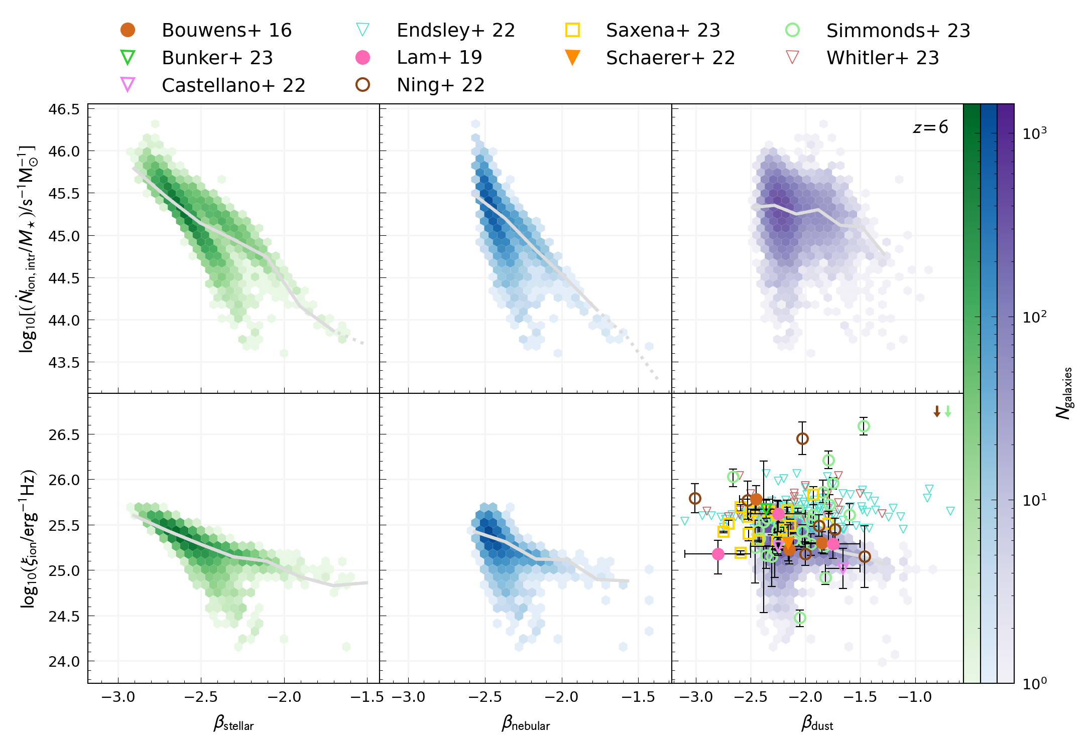
Figure 9: Specific emissivity (upper panels) and ionising photon production efficiency (lower panels) plotted against the UV-continuum slope, obtained from pure stellar SEDs (left column), stellar SEDs with nebular emission (middle column), stellar SEDs with nebular emission and dust (right column). Hex bins show the distribution of galaxies in Flares at $z=6$ and trend lines show the weighted median. Observations are represented by scatter points, with the same classification by marker style and fill as in Figure 7. Arrows indicate how values may change when accounting for dust (for measurements by Ning et al., 2022; Simmonds et al., 2023). To maintain readability, error bars have been left out for measurements by Endsley et al. (2022) and Whitler et al. (2023).

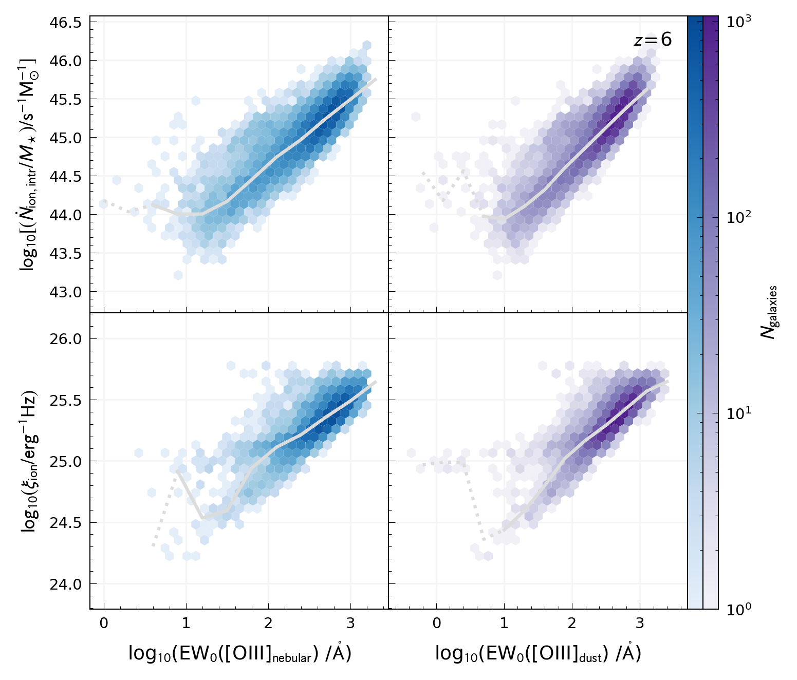
Figure 10: Specific emissivity (upper panels) and ionising photon production efficiency (lower panels) plotted against the intrinsic (left column) and dust-attenuated (right column) [O iii] EW values. Hex bins show the distribution of galaxies in Flares at $z=6$ and trend lines show the weighted median. Observations are represented by scatter points.

5.4.1 UV-continuum slope

Figure 9 shows how the specific emissivity and production efficiency vary with the UV-continuum slope, $\beta$. Moving from the leftmost column to the right shows the evolution of $\beta$ when nebular emission and dust are included in our SED modelling (thus the rightmost column shows the observed $\beta$). The general trend is that galaxies in Flares with high specific emissivities and production efficiencies tend to have bluer UV-continuum slopes. This trend is more evident when considering the pure stellar UV slopes, and subject to large amounts of scatter when considering the dust-attenuated values of $\beta$. We observe two distinct populations of galaxies, forming two branches in the distribution. The lower branch consists of low stellar mass galaxies with low metallicities, while the upper branch consists of more massive galaxies with higher metallicities. As we go through our analysis, Figure 16 in the Appendix may be of interest to the reader, as it contains identical plots to Figure 9 but coloured by specific star formation rate, metallicity, and stellar mass.

To understand how the relation between the production efficiency and the observed value of $\beta$ (i.e. with nebular emission and dust) comes about, it is useful to first start with the UV slope derived from pure stellar SEDs. The lower left panel of Figure 9 shows that galaxies with the highest production efficiencies have the bluest pure stellar UV slopes. This is as expected, since both phenomena are correlated with the presence of young, massive stars, and indeed we find that these galaxies have the highest specific star formation rates. The two ‘tails’ we observe at redder values of $\beta$ are due to a difference in metallicity, as mentioned earlier – the upper branch of galaxies has a higher metallicity, which leads to redder values of $\beta$. Due to the strong mass-metallicity relation in Flares, we find that galaxies in the upper branch are more massive as well.

Moving to the lower middle panel, we see the evolution of $\beta$ when nebular emission is added. Note that we are only looking at the change in values of $\beta$, since the specific emissivity $\dot{N}_{\rm ion,intr}/M_{\star}$ and the production efficiency $\xi_{\rm ion}$ remain the same throughout. The main difference is that the highly star-forming galaxies with high production efficiencies now have redder UV slopes, as a result of nebular continuum emission (Byler et al., 2017; Topping et al., 2022).

Finally, moving on to the lower right panel, we see that the effect of dust is also to redden the UV slopes. The change is more pronounced for the upper branch of galaxies with high stellar masses and metallicities, as they tend to be more dusty. The addition of dust increases the amount of scatter in the relation – in the case of the specific emissivity, this causes the median line to flatten considerably.

The predictions from Flares overlap with a number of observations (Bouwens et al., 2016; Castellano et al., 2022; Schaerer et al., 2022; Bunker et al., 2023; Saxena et al., 2023; Simmonds et al., 2023), but do not reproduce the elevated production efficiencies or the bluest values of $\beta$ ($\beta\sim-3.0$). The latter is due to the fact that all the ionising photons produced by a galaxy are reprocessed through the nebula, as described in Section 3.3.2. Previous studies have predicted an increase in $\xi_{\rm ion}$ for the bluest UV slopes (Robertson et al., 2013; Duncan & Conselice, 2015). None of the observations plotted in Figure 9 show a clear trend. This could be in part due to samples being biased towards highly star-forming galaxies, such as in the study by Endsley et al. (2022). More inclusive survey samples, or perhaps a greater variety of surveys, would enable us to come to a stronger conclusion.

5.4.2 [O iii] equivalent width

Observational studies have found a positive correlation between [O iii] emission line strength and the ionising photon production efficiency of galaxies (Chevallard et al., 2018; Reddy et al., 2018; Tang et al., 2019; Emami et al., 2020; Castellano et al., 2023). This trend is also observed in Flares. We define the [O iii] equivalent width (EW) as the combined equivalent widths of the [O iii] doublet ([O iii]$\lambda\lambda$4960,5008Å). Figure 10 shows that the specific emissivity and production efficiency of a galaxy is positively correlated with the [O iii] EW, although the relation is subject to scatter. The positive correlation can be explained by the fact that [O iii] emission is primarily driven by ionising radiation from young, massive stars, while the underlying optical continuum is boosted by emission from older stars as well. Thus the optical continuum can be interpreted as a ‘normalising’ factor in the definition of the equivalent width. The distributions we observe are not strongly affected by dust – this is something Wilkins et al. (2023a) also found in their paper analysing the [O iii] emission of galaxies in Flares. We note that the gradient of the relation is metallicity-dependent. In fact, the spread of values seen in Figure 10 consists of a low metallicity population and a high metallicity population, with different relations to the [O iii] EW. More detail on this can be found in Section A.3 of the Appendix.

A solar abundance pattern was adopted to align with the BPASS SPS model that we use for our stellar SEDs. We note that high-redshift galaxies are $\alpha$-enhanced, meaning that they are likely to contain a higher proportion of $\alpha$-elements, such as oxygen (Steidel et al., 2016; Strom et al., 2022; Cullen et al., 2021; Byrne et al., 2022). Wilkins et al. (2023a) estimate a potential increase in the [O iii] fluxes of $\sim 0.1$ dex, when $\alpha$-enhancement is accounted for.

5.5 Dust-attenuated production efficiency

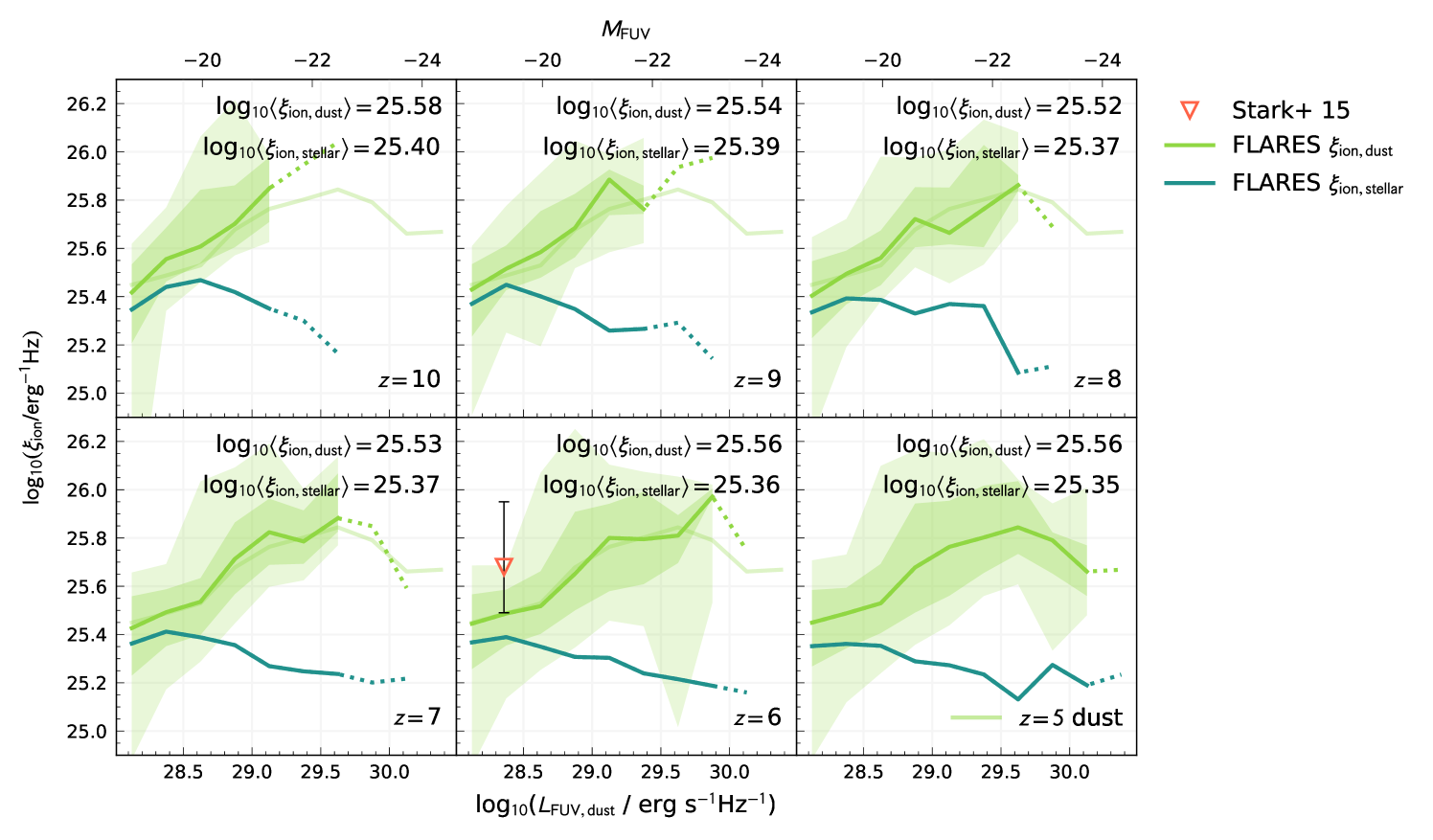
Figure 11: Ionising photon production efficiency of galaxies in Flares, defined in terms of dust-attenuated and pure stellar far-UV luminosity ($\xi_{\rm ion,dust}$ and $\xi_{\rm ion,stellar}$ in green and blue respectively). Trend lines show the weighted median production efficiencies, with dotted lines representing bins containing fewer than 10 galaxies. Shaded regions denote the 1 and $2\sigma$ range of $\xi_{\rm ion,dust}$. Observations are represented by scatter points.

So far, we have defined the ionising photon production efficiency following Equation 3, choosing to normalise the ionising emissivity of a galaxy by its intrinsic far-UV luminosity. From the perspective of forward-modelling from simulations, this means that no nebular emission or dust is modelled – only stellar SEDs are used. For the sake of clarity, in this subsection we will label this value $\xi_{\rm ion,stellar}$, i.e. $\xi_{\rm ion}=\xi_{\rm ion,stellar}$. On the other hand, obtaining the intrinsic luminosity from observations requires an assumption of the dust model, which can be an uncertain parameter (e.g. Ferrara et al., 2016; Behrens et al., 2018; De Barros et al., 2019; Vijayan et al., 2023).

Alternatively, one can study the production efficiency defined using the dust-attenuated UV luminosity:

$$\xi_{\rm ion,dust}=\frac{\dot{N}_{\rm ion,intr}}{L_{\rm UV,dust}},$$ (9)

where the subscript ‘dust’ is now used to clarify that the UV luminosity is dust-attenuated. Forward-modelling from simulations would thus require additional modelling assumptions, in the incorporation of nebular emission and dust, in order to obtain $L_{\rm UV,dust}$. On the other hand, working with $\xi_{\rm ion,dust}$ can reduce the modelling assumptions made in observing the production efficiency, since the observed far-UV luminosity can be used without correcting for dust. This is more so the case when estimating the production efficiency from line fluxes, since an intrinsic SPS model has to be assumed to obtain $\dot{N}_{\rm ion,intr}$ from SED fitting. We note that using this definition does not completely remove the need for dust corrections – estimating $\dot{N}_{\rm ion,intr}$ from line fluxes would require dust corrections in order to obtain the intrinsic flux.

Figure 11 compares predictions for $\xi_{\rm ion,dust}$ and $\xi_{\rm ion,stellar}$ in Flares. We see no dependence of $\xi_{\rm ion,dust}$ on redshift, with median values hovering around $\log_{10}(\xi_{\rm ion,dust}\rm{/erg^{-1}Hz})=25.55$. $\xi_{\rm ion,dust}$ follows a reverse trend to $\xi_{\rm ion,stellar}$, increasing from faint luminosities to $\log_{10}(L_{\rm FUV,dust}\rm{/erg\,s^{-1}\,Hz^{-1}})\sim 29.5$, after which values plateau or tentatively decrease. The ratio between $\xi_{\rm ion,dust}$ and $\xi_{\rm ion,stellar}$ roughly follows the trend in dust attenuation, by definition. Figure 9 of Vijayan et al. (2021) shows the dust attenuation in the far-UV of galaxies in Flares, as a function of far-UV magnitude. Brighter, more massive galaxies tend to be more highly attenuated, as they have undergone longer periods of star formation that enrich the ISM and produce dust. However, the attenuation stops increasing at $\log_{10}(L_{\rm FUV,dust}\rm{/erg\,s^{-1}\,Hz^{-1}})\sim 29.5$ ($M_{\rm FUV}\sim 22$), which is also where we observe the downturn in $\xi_{\rm ion,dust}$.

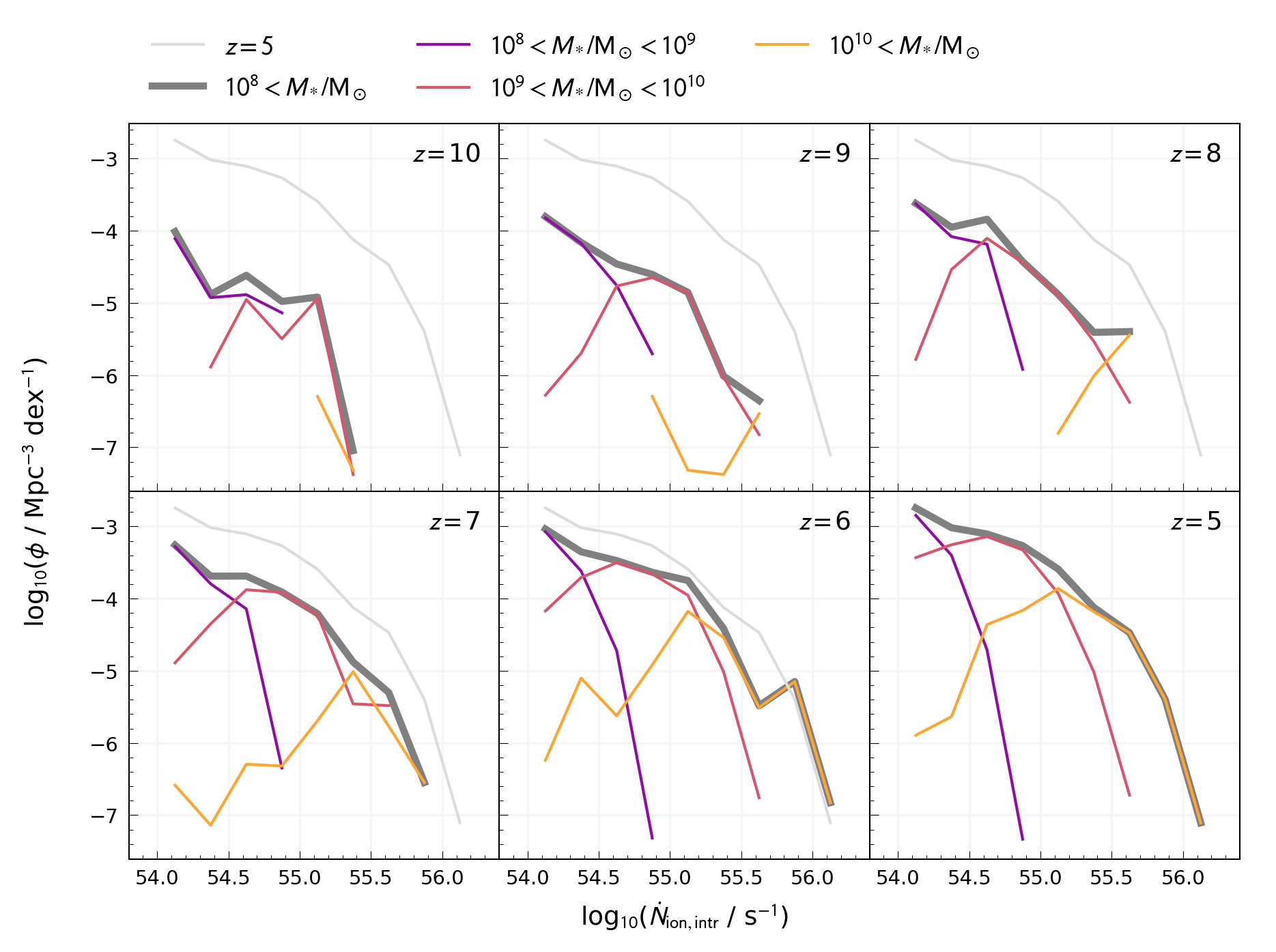
Figure 12: Lyman-continuum luminosity function (stellar contribution only) for galaxies in Flares. In dark grey is the luminosity function for all galaxies with ionising emissivity $\dot{N}_{\rm ion,intr}>10^{54}\rm{s^{-1}}$, which roughly corresponds to a stellar mass cut of $M_{*}>10^{8}\rm{M_{\odot}}$. This population of galaxies has been binned by stellar mass, and the contribution from each mass bin plotted as well (in order of increasing stellar mass: purple, red, yellow). As a reference, the $z=5$ function is plotted in light grey.

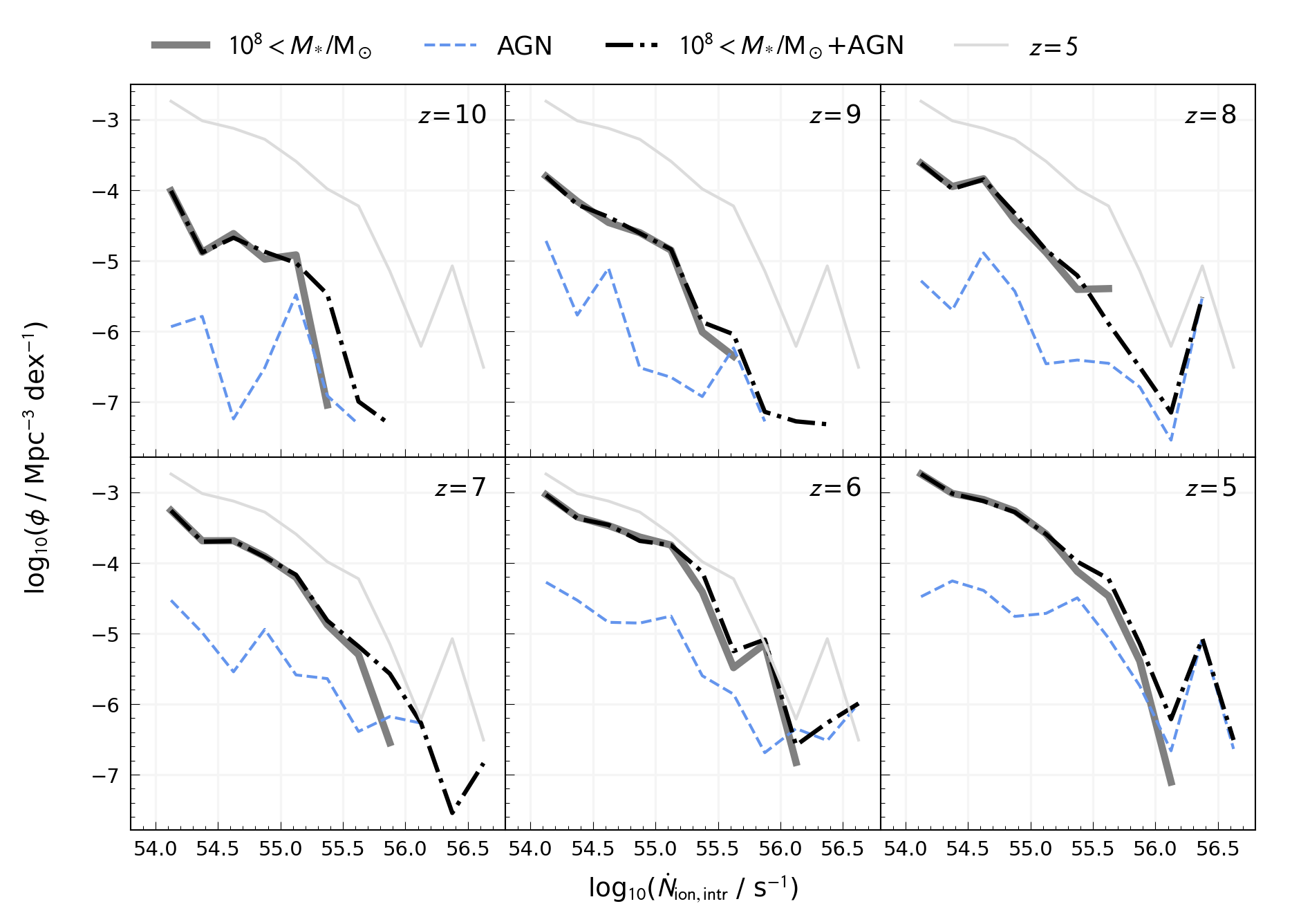
Figure 13: Lyman-continuum luminosity function for galaxies in Flares, considering all galaxies with stellar mass $M_{*}>10^{8}\rm{M_{\odot}}$. The solid, dark grey line shows the stellar luminosity function, the dashed blue line shows the AGN luminosity function, and the dash-dotted black line shows the luminosity function total luminosity (i.e. stellar $+$ AGN). As a reference, the $z=5$ function is plotted in light grey.

6 Intrinsic ionising emissivity

In this section, we study the intrinsic ionising emissivity of galaxies in Flares, analysing the intrinsic LyC luminosity function and the relative contributions to the total ionising emissivity from different populations in our sample.

6.1 LyC luminosity function

Figure 12 shows the evolution of the LyC luminosity function with redshift (note that only the contribution from stars is shown). The contributions from different stellar mass bins are also shown, with the higher mass bins dominating at the brighter end of the luminosity function. We showed in Sections 4 and 5 that massive galaxies tend to be less efficient at producing ionising radiation. Despite this, their large stellar populations compensate for the low efficiency, and we find that the total ionising emissivity of a galaxy increases with stellar mass. Hence, the LyC luminosity function is strongly governed by the galaxy stellar mass function – the negative slopes observed in Figure 12 are due to the decreasing number of galaxies as we go to higher stellar masses.

The AGN LyC luminosity function is shown as the dotted blue line in Figure 13 (we refer the reader to Kuusisto et al., in prep for information on how AGN emission is modelled in Flares). At lower emissivities, the AGN luminosity function is small compared to that of stars. However, AGN dominate the bright end of the LyC luminosity function – after the rapid drop in the stellar luminosity function at $\rm{log}_{10}(\dot{N}_{\rm ion}/s^{-1})\sim 56$, we find it is the more gently decreasing AGN luminosity function that extends the combined emissivity to higher values (by $\sim 0.5$ dex).

6.2 Contribution from different populations

Figure 14 shows the combined ionising emissivity per unit volume of different populations discussed in the previous section (6.1), obtained by taking the integral of the LyC luminosity function. There is an increase in the total emissivity (black line) as redshift decreases, as one would expect, since the number of galaxies is increasing due to hierarchical assembly. Across all considered redshifts, from $z=10-5$, the contribution from AGN is small but still significant, generally providing between $10-20$% of the total emissivity (lower panel of Figure 14). The main source of ionising photons is lower mass galaxies – from $z=10-7$, galaxies with $M_{*}=10^{8}-10^{9}\,\rm{M_{\odot}}$ contribute the most, with $M_{*}=10^{9}-10^{10}\,\rm{M_{\odot}}$ galaxies catching up at lower redshifts.

We note that these comparisons of the fractional contribution to the emissivity are relative statements that depend on the galaxy population being studied. If the analysis were extended to galaxies with stellar masses below the resolution in Flares, the fractional contribution from AGN would decrease, as AGN are less common in low mass galaxies.

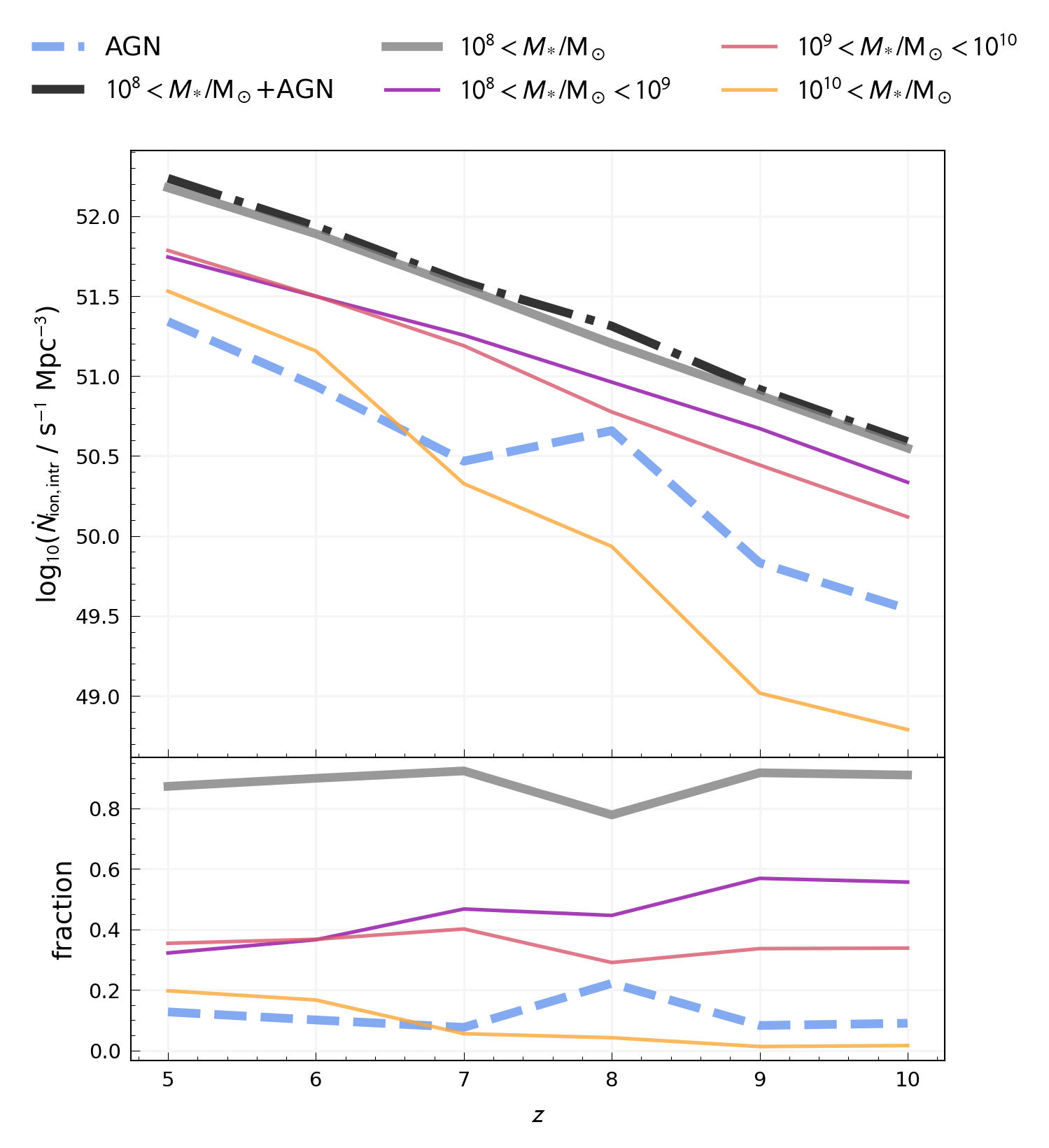
Figure 14: Top panel: redshift evolution of the total ionising emissivity per Mpc^-3 of Flares galaxies. Solid lines show the stellar contribution – in dark grey is the contribution from galaxies with stellar mass $M_{*}>10^{8}\rm{M_{\odot}}$, in purple, red and yellow are the contributions from different stellar mass bins. The dashed blue line shows the AGN contribution, and the dash-dotted black line shows the total contribution (i.e. stellar $+$ AGN). Bottom panel: fraction of the total emissivity contributed by each population as a function of redshift.

7 Conclusions

In this paper, we have used the Flare simulations to make predictions for the ionising properties of galaxies, namely, their intrinsic ionising emissivity and ionising photon production efficiency. We began by using simple toy models to explore how these two quantities vary with SFH, metallicity, choice of SPS model, and IMF. This provided a theoretical foundation for our main analysis on galaxies in Flares, which naturally have more realistic properties. We explored how the specific emissivity is linked to the physical properties of galaxies, and how the production efficiency relates to observable properties. We also compared our predictions to recent observational estimates. Our findings are summarised below:

• Using simple toy models, we show that the specific emissivity and production efficiency are sensitive to the SFH and metallicity of galaxies. In our examples, all SFHs cause a decline in both quantities. However, an increasing exponential SFH eventually leads to a plateau in their values, while an instantaneous SFH results in an immediate, sharp decline. Trends for a CSFH and decreasing exponential SFH fall between these two extremes. We also find that the specific emissivity and production efficiency strongly depend on the SPS library and IMF used.

• The specific ionising emissivity of galaxies in Flares is strongly correlated with their specific star formation rate and negatively correlated with age, which we define as the initial mass-weighted median stellar age. This is because young, massive stars are the dominant source of ionising photons in a stellar population.

• The specific ionising emissivity of galaxies in Flares shows little evolution at at low metallicities. We observe a peak in the specific emissivity at $Z_{\star}\sim 10^{-2.5}$, after which there is a stronger trend of decreasing specific emissivity with increasing metallicity. The general trend can be attributed to the BPASS SPS model that we use, however, the peak is characteristic of galaxies in Flares – we find that galaxies with stellar masses $M_{\star}\sim 10^{9.5}\,\rm{M_{\odot}}$ (corresponding to a metallicity of $Z_{\star}\sim 10^{-2.5}$) tend to undergo a burst of star formation in their cores, increasing the specific star formation rate and hence the specific emissivity.

• Galaxies in Flares with stellar masses $M_{\star}\sim 10^{9.5}\,\rm{M_{\odot}}$ exhibit a trend of decreasing specific emissivity with increasing stellar mass. This is due to the combined effects of increasing age and metallicity with increasing stellar mass, with metallicity likely playing a bigger role due to the weaker evolution of age with stellar mass.

• The ionising photon production efficiency of galaxies in Flares generally increases as we go to lower far-UV luminosities. As the FUV luminosity of galaxies in Flares is strongly correlated with stellar mass, this trend parallels that of the specific emissivity with stellar mass, and likewise can be attributed to the effects of age and metallicity.

• We find a trend of decreasing production efficiency as redshift decreases, due to the effect of increasing age.

• Flares predicts values of the production efficiency that are comparable with previous theoretical studies (Wilkins et al., 2016; Ceverino et al., 2019; Yung et al., 2020a). On the other hand, observations of the production efficiency tend to be around or higher than the values predicted by Flares. There are several possible reasons for this discrepancy. On the theoretical side, we are limited by the mass resolution of our model, and have not included the contribution from AGN. As for observations, we note that a variety of methods has been used to obtain the production efficiency. In general, measurements made using spectroscopically-obtained H$\alpha$ or H$\beta$ line fluxes can be considered more robust than those obtained using SED fitting, or the line fluxes estimated from colours. We note that the choice of SPS model and dust model may have a strong influence on predicted values.

• The production efficiency of galaxies in Flares generally decreases as we go to redder values of the UV continuum slope $\beta$, however this trend is subject to scatter and has a metallicity-dependent gradient. We observe a positive correlation between the production efficiency and the [O iii] EW, although this relation is also subject to scatter.

• Despite having lower specific ionising emissivities, it is the most massive galaxies that have the highest ionising emissivities, dominating the bright end of the intrinsic stellar Lyman-continuum luminosity function. We show that the luminosity function decreases at higher emissivities, governed by the galaxy stellar mass function. When including the AGN component, we find that AGN contribute relatively little compared to stars, but extend the luminosity function to higher emissivities.

• Considering our galaxy population at $M_{\star}>10^{8}\,\rm{M_{\odot}}$, we find that the lowest mass galaxies contribute the most to the total ionising emissivity, due to their large population size. In general, the fractional contribution decreases with increasing stellar mass.

The ionising emissivity and ionising photon production efficiency are important parameters in linking the formation and evolution of galaxies to the history of reionisation. In this paper, we have provided theoretical insight into these parameters, and made predictions based on the standard cosmological model. In large part thanks to the operations of JWST, the number of robust observational measurements of the production efficiency is steadily increasing, and will continue to do so in the coming years, enabling better constraints on the ionising properties of high-redshift galaxies.

Data Availability

Some of the Flares data published this paper is publicly available at https://github.com/louiseseeyave/flares_lyc. Data from the wider Flares project is available at https://flaresimulations.github.io/#data.

Appendix A Ionising photon production efficiency

A.1 Stellar mass

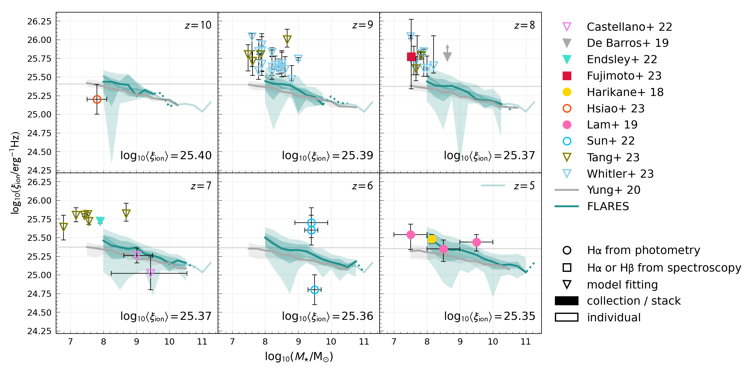
Figure 15: Ionising photon production efficiency as a function of stellar mass, for redshifts $5-10$. Trend lines and their colour-associated shaded regions represent the median and 1$\sigma$ range from theoretical models: in grey is the median trend from Yung et al. (2020a); in blue are the weighted median trends from Flares. The faint, horizontal grey line indicates the weighted mean of the Flares sample at each redshift. The translucent blue line plotted across all panels shows the Flares weighted median at $z=5$. Observations are displayed as scatter points: those with a transparent fill are measurements of individual galaxies; those with a solid fill are aggregated values, representing either stacks or collections of galaxies; circular and square data points represent measurements of the production efficiency obtained using Balmer emission line fluxes fluxes from photometry and spectroscopy respectively; triangular data points represent measurements of the production efficiency obtained from model fitting (this is a broad term that encompasses SED fitting). Observations are plotted in the panel corresponding to the nearest integer redshift.

Figure 15 shows the production efficiency as a function of stellar mass for galaxies in Flares. The production efficiency generally decreases as stellar mass increases, similar to the trend seen in Figure 7. Also plotted are predictions from Yung et al. (2020a), and measurements from several observational studies. Note that for the sake of readability, horizontal error bars have been omitted for measurements by Tang et al. (2023) and Whitler et al. (2023). In general, Flares predicts slightly higher median values of the production efficiency than Yung et al. (2020a), by $\sim 0.1$ dex. Both Flares and Yung et al. (2020a) use v2.2.1 of the BPASS SPS library.

A.2 UV-continuum slope

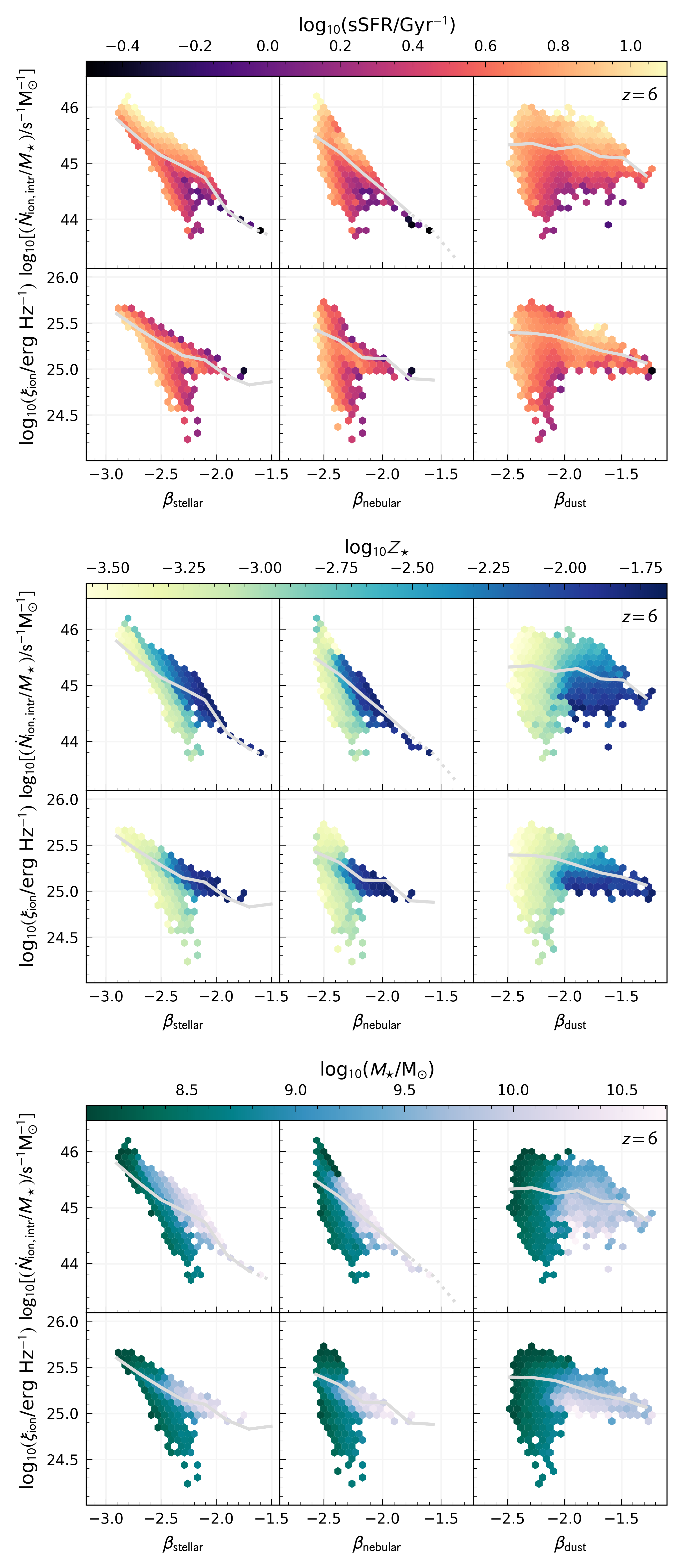
Figure 16: These three plots are identical except for the quantity used to colour the hex bins. Each plot shows the specific emissivity (upper panels) and ionising photon production efficiency (lower panels) plotted against the UV-continuum slope, obtained from pure stellar SEDs (left column), stellar SEDs with nebular emission (middle column), stellar SEDs with nebular emission and dust (right column). Hex bins show the distribution of galaxies in Flares at $z=6$, and are coloured by the mean specific star formation rate (top plot), stellar metallicity (middle plot), and stellar mass (bottom plot). Trend lines show the weighted median.

Figure 16 shows the specific emissivity and production efficiency as a function of the UV-continuum slope. This plot is supplementary to the discussion in Section 5.4.1.

A.3 [O iii] equivalent width

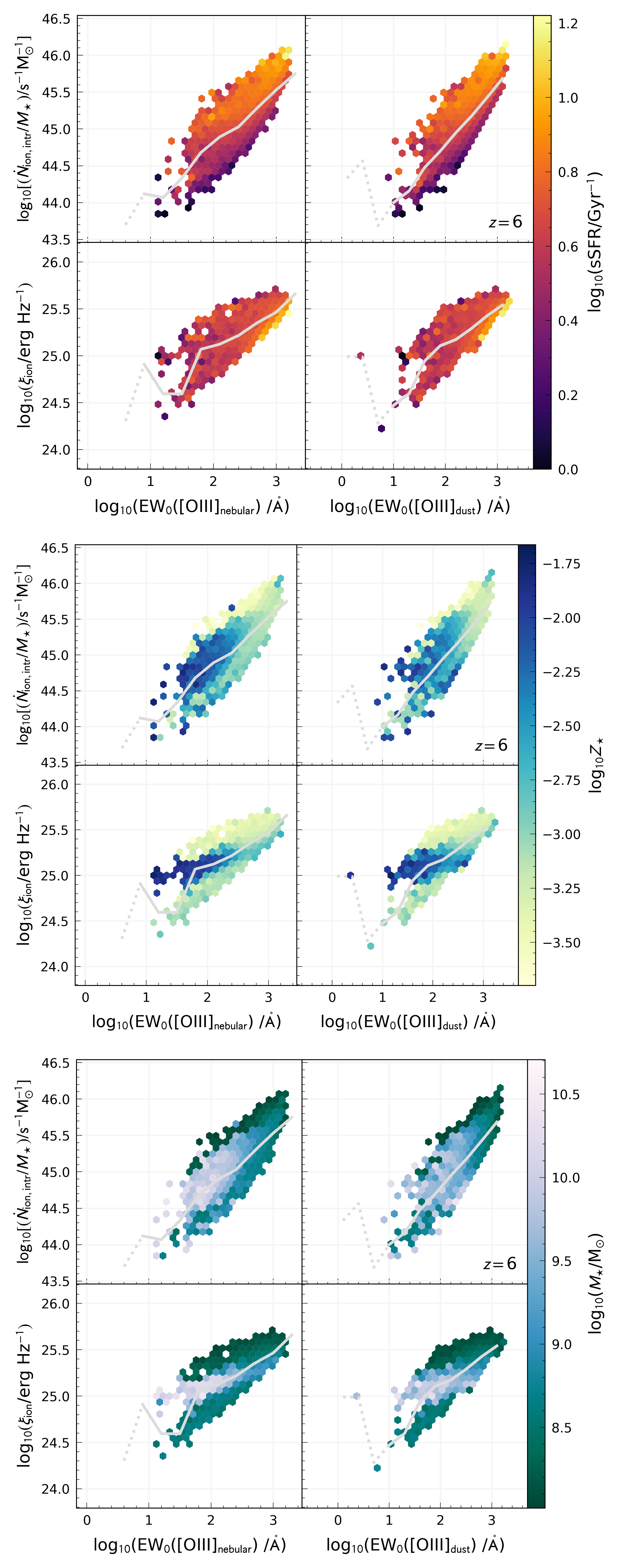
Figure 17: These three plots are identical except for the quantity used to colour the hex bins. Each plot shows the specific emissivity (upper panels) and ionising photon production efficiency (lower panels) plotted against the intrinsic (left column) and dust-attenuated (right column) [O iii] EW values. Hex bins show the distribution of galaxies in Flares at $z=6$, and are coloured by the mean specific star formation rate (top plot), stellar metallicity (middle plot), and stellar mass (bottom plot). Trend lines show the weighted median.

Two separate galaxy populations are observed in the relationship between the [O iii] equivalent width (EW) and $\xi_{\rm ion}$. This becomes clearer when looking at the middle and bottom plots in Figure 17 – there is a population of galaxies with higher stellar masses and metallicities that exhibits a weaker trend with [O iii] EW. This is due to the effect of metallicity – Wilkins et al. (2023a) show that the [O iii] EW increases with metallicity (due to the increasing Oxygen abundance) until $Z_{\star}\sim 10^{-2.5}$, and then decreases as a result of higher metallicities decreasing the amount of ionising radiation produced (second panel of Figure 5). The population of galaxies exhibiting this weaker trend has metallicities above this critical value. We find that the two populations are not so distinct when considering the specific ionising emissivity.

References

- Astropy Collaboration et al. (2022) Astropy Collaboration et al., 2022, ApJ, 935, 167
- Barnes et al. (2017a) Barnes D. J., Kay S. T., Henson M. A., McCarthy I. G., Schaye J., Jenkins A., 2017a, MNRAS, 465, 213
- Barnes et al. (2017b) Barnes D. J., et al., 2017b, MNRAS, 471, 1088
- Behrens et al. (2018) Behrens C., Pallottini A., Ferrara A., Gallerani S., Vallini L., 2018, MNRAS, 477, 552
- Bera et al. (2022) Bera A., Hassan S., Smith A., Cen R., Garaldi E., Kannan R., Vogelsberger M., 2022, arXiv e-prints, p. arXiv:2209.14312
- Bosman et al. (2022) Bosman S. E. I., et al., 2022, MNRAS, 514, 55
- Bouwens et al. (2015) Bouwens R. J., et al., 2015, ApJ, 803, 34
- Bouwens et al. (2016) Bouwens R. J., Smit R., Labbé I., Franx M., Caruana J., Oesch P., Stefanon M., Rasappu N., 2016, ApJ, 831, 176
- Bruzual & Charlot (2003) Bruzual G., Charlot S., 2003, MNRAS, 344, 1000
- Bunker et al. (2023) Bunker A. J., et al., 2023, arXiv e-prints, p. arXiv:2302.07256
- Byler et al. (2017) Byler N., Dalcanton J. J., Conroy C., Johnson B. D., 2017, ApJ, 840, 44
- Byrne et al. (2022) Byrne C. M., Stanway E. R., Eldridge J. J., McSwiney L., Townsend O. T., 2022, MNRAS, 512, 5329
- Calzetti et al. (2000) Calzetti D., Armus L., Bohlin R. C., Kinney A. L., Koornneef J., Storchi-Bergmann T., 2000, ApJ, 533, 682
- Castellano et al. (2022) Castellano M., et al., 2022, A&A, 662, A115
- Castellano et al. (2023) Castellano M., et al., 2023, arXiv e-prints, p. arXiv:2305.13364
- Ceverino et al. (2019) Ceverino D., Klessen R. S., Glover S. C. O., 2019, MNRAS, 484, 1366
- Chabrier (2003) Chabrier G., 2003, PASP, 115, 763
- Charlot & Fall (2000) Charlot S., Fall S. M., 2000, ApJ, 539, 718
- Chevallard & Charlot (2016) Chevallard J., Charlot S., 2016, MNRAS, 462, 1415
- Chevallard et al. (2013) Chevallard J., Charlot S., Wandelt B., Wild V., 2013, MNRAS, 432, 2061
- Chevallard et al. (2018) Chevallard J., et al., 2018, MNRAS, 479, 3264
- Chiang et al. (2013) Chiang Y.-K., Overzier R., Gebhardt K., 2013, ApJ, 779, 127
- Choudhury et al. (2021) Choudhury T. R., Paranjape A., Bosman S. E. I., 2021, MNRAS, 501, 5782
- Conroy & Gunn (2010) Conroy C., Gunn J. E., 2010, FSPS: Flexible Stellar Population Synthesis, Astrophysics Source Code Library, record ascl:1010.043 (ascl:1010.043)
- Conroy et al. (2009) Conroy C., Gunn J. E., White M., 2009, ApJ, 699, 486
- Crain et al. (2015) Crain R. A., et al., 2015, MNRAS, 450, 1937
- Cullen et al. (2021) Cullen F., et al., 2021, MNRAS, 505, 903
- Davis et al. (1985) Davis M., Efstathiou G., Frenk C. S., White S. D. M., 1985, ApJ, 292, 371
- Dayal & Ferrara (2018) Dayal P., Ferrara A., 2018, Phys. Rep., 780, 1
- Dayal et al. (2020) Dayal P., et al., 2020, MNRAS, 495, 3065
- De Barros et al. (2019) De Barros S., Oesch P. A., Labbé I., Stefanon M., González V., Smit R., Bouwens R. J., Illingworth G. D., 2019, MNRAS, 489, 2355
- Duncan & Conselice (2015) Duncan K., Conselice C. J., 2015, MNRAS, 451, 2030
- Eilers et al. (2018) Eilers A.-C., Davies F. B., Hennawi J. F., 2018, ApJ, 864, 53
- Eldridge & Stanway (2020) Eldridge J. J., Stanway E. R., 2020, arXiv e-prints, p. arXiv:2005.11883
- Eldridge et al. (2008) Eldridge J. J., Izzard R. G., Tout C. A., 2008, MNRAS, 384, 1109
- Eldridge et al. (2017) Eldridge J. J., Stanway E. R., Xiao L., McClelland L. A. S., Taylor G., Ng M., Greis S. M. L., Bray J. C., 2017, Publ. Astron. Soc. Australia, 34, e058
- Emami et al. (2020) Emami N., Siana B., Alavi A., Gburek T., Freeman W. R., Richard J., Weisz D. R., Stark D. P., 2020, ApJ, 895, 116
- Endsley et al. (2021) Endsley R., Stark D. P., Charlot S., Chevallard J., Robertson B., Bouwens R. J., Stefanon M., 2021, MNRAS, 502, 6044
- Endsley et al. (2022) Endsley R., Stark D. P., Whitler L., Topping M. W., Chen Z., Plat A., Chisholm J., Charlot S., 2022, arXiv e-prints, p. arXiv:2208.14999
- Faisst et al. (2019) Faisst A. L., Capak P. L., Emami N., Tacchella S., Larson K. L., 2019, ApJ, 884, 133
- Fan et al. (2006) Fan X., Carilli C. L., Keating B., 2006, ARA&A, 44, 415
- Ferland et al. (2017) Ferland G. J., et al., 2017, Rev. Mex. Astron. Astrofis., 53, 385
- Ferrara et al. (2016) Ferrara A., Viti S., Ceccarelli C., 2016, MNRAS, 463, L112
- Finkelstein et al. (2019) Finkelstein S. L., et al., 2019, ApJ, 879, 36
- Fujimoto et al. (2023) Fujimoto S., et al., 2023, arXiv e-prints, p. arXiv:2301.09482
- Götberg et al. (2019) Götberg Y., de Mink S. E., Groh J. H., Leitherer C., Norman C., 2019, A&A, 629, A134
- Gutkin et al. (2016) Gutkin J., Charlot S., Bruzual G., 2016, MNRAS, 462, 1757
- Harikane et al. (2018) Harikane Y., et al., 2018, ApJ, 859, 84
- Hsiao et al. (2023) Hsiao T. Y.-Y., et al., 2023, arXiv e-prints, p. arXiv:2305.03042
- Hunter (2007) Hunter J. D., 2007, Computing in Science & Engineering, 9, 90
- Jones et al. (2022) Jones G. T., Stanway E. R., Carnall A. C., 2022, MNRAS, 514, 5706
- Lam et al. (2019) Lam D., et al., 2019, A&A, 627, A164
- Leitherer & Heckman (1995) Leitherer C., Heckman T. M., 1995, ApJS, 96, 9
- Lewis et al. (2020) Lewis J. S. W., et al., 2020, MNRAS, 496, 4342
- Lin et al. (2023) Lin Y.-H., et al., 2023, arXiv e-prints, p. arXiv:2303.04572
- Lovell et al. (2018) Lovell C. C., Thomas P. A., Wilkins S. M., 2018, MNRAS, 474, 4612
- Lovell et al. (2021) Lovell C. C., Vijayan A. P., Thomas P. A., Wilkins S. M., Barnes D. J., Irodotou D., Roper W., 2021, MNRAS, 500, 2127
- Lovell et al. (2022) Lovell C. C., et al., 2022, arXiv e-prints, p. arXiv:2211.07540
- Ma et al. (2016) Ma X., Hopkins P. F., Kasen D., Quataert E., Faucher-Giguère C.-A., Kereš D., Murray N., Strom A., 2016, MNRAS, 459, 3614
- Maseda et al. (2020) Maseda M. V., et al., 2020, MNRAS, 493, 5120
- Matthee et al. (2017) Matthee J., Sobral D., Best P., Khostovan A. A., Oteo I., Bouwens R., Röttgering H., 2017, MNRAS, 465, 3637
- Matthee et al. (2022) Matthee J., Mackenzie R., Simcoe R. A., Kashino D., Lilly S. J., Bordoloi R., Eilers A.-C., 2022, arXiv e-prints, p. arXiv:2211.08255
- McGreer et al. (2015) McGreer I. D., Mesinger A., D’Odorico V., 2015, MNRAS, 447, 499
- Mutch et al. (2023) Mutch S. J., Greig B., Qin Y., Poole G. B., Wyithe J. S. B., 2023, arXiv e-prints, p. arXiv:2303.07378
- Nakajima et al. (2016) Nakajima K., Ellis R. S., Iwata I., Inoue A. K., Kusakabe H., Ouchi M., Robertson B. E., 2016, ApJ, 831, L9
- Ning et al. (2022) Ning Y., Cai Z., Jiang L., Lin X., Fu S., Spinoso D., 2022, arXiv e-prints, p. arXiv:2211.13620
- Onoue et al. (2017) Onoue M., et al., 2017, ApJ, 847, L15
- Pei (1992) Pei Y. C., 1992, ApJ, 395, 130
- Prieto-Lyon et al. (2023) Prieto-Lyon G., et al., 2023, A&A, 672, A186
- Reddy et al. (2018) Reddy N. A., et al., 2018, ApJ, 869, 92
- Robertson (2022) Robertson B. E., 2022, ARA&A, 60, 121
- Robertson et al. (2013) Robertson B. E., et al., 2013, ApJ, 768, 71
- Roper et al. (2022) Roper W. J., Lovell C. C., Vijayan A. P., Marshall M. A., Irodotou D., Kuusisto J. K., Thomas P. A., Wilkins S. M., 2022, MNRAS, 514, 1921
- Roper et al. (2023) Roper W. J., et al., 2023, arXiv e-prints, p. arXiv:2301.05228
- Saxena et al. (2023) Saxena A., et al., 2023, arXiv e-prints, p. arXiv:2306.04536
- Schaerer (2003) Schaerer D., 2003, A&A, 397, 527
- Schaerer et al. (2022) Schaerer D., Marques-Chaves R., Barrufet L., Oesch P., Izotov Y. I., Naidu R., Guseva N. G., Brammer G., 2022, A&A, 665, L4
- Schaye et al. (2015) Schaye J., et al., 2015, MNRAS, 446, 521
- Shivaei et al. (2018) Shivaei I., et al., 2018, ApJ, 855, 42
- Simmonds et al. (2023) Simmonds C., et al., 2023, arXiv e-prints, p. arXiv:2303.07931
- Springel et al. (2001) Springel V., White S. D. M., Tormen G., Kauffmann G., 2001, MNRAS, 328, 726
- Stanway & Eldridge (2018) Stanway E. R., Eldridge J. J., 2018, MNRAS, 479, 75
- Stanway et al. (2016) Stanway E. R., Eldridge J. J., Becker G. D., 2016, MNRAS, 456, 485
- Stark et al. (2015) Stark D. P., et al., 2015, MNRAS, 454, 1393
- Stark et al. (2017) Stark D. P., et al., 2017, MNRAS, 464, 469
- Stefanon et al. (2022) Stefanon M., Bouwens R. J., Illingworth G. D., Labbé I., Oesch P. A., Gonzalez V., 2022, ApJ, 935, 94
- Steidel et al. (2016) Steidel C. C., Strom A. L., Pettini M., Rudie G. C., Reddy N. A., Trainor R. F., 2016, ApJ, 826, 159
- Strom et al. (2022) Strom A. L., Rudie G. C., Steidel C. C., Trainor R. F., 2022, ApJ, 925, 116
- Sun et al. (2022) Sun F., et al., 2022, arXiv e-prints, p. arXiv:2209.03374
- Tang et al. (2019) Tang M., Stark D. P., Chevallard J., Charlot S., 2019, MNRAS, 489, 2572
- Tang et al. (2023) Tang M., et al., 2023, arXiv e-prints, p. arXiv:2301.07072
- Thomas et al. (2023) Thomas P. A., Lovell C. C., Maltz M. G. A., Vijayan A. P., Wilkins S. M., Irodotou D., Roper W. J., Seeyave L., 2023, arXiv e-prints, p. arXiv:2301.09510
- Topping et al. (2022) Topping M. W., Stark D. P., Endsley R., Plat A., Whitler L., Chen Z., Charlot S., 2022, ApJ, 941, 153
- Vijayan et al. (2019) Vijayan A. P., Clay S. J., Thomas P. A., Yates R. M., Wilkins S. M., Henriques B. M., 2019, MNRAS, 489, 4072
- Vijayan et al. (2021) Vijayan A. P., Lovell C. C., Wilkins S. M., Thomas P. A., Barnes D. J., Irodotou D., Kuusisto J., Roper W. J., 2021, MNRAS, 501, 3289
- Vijayan et al. (2023) Vijayan A. P., Thomas P. A., Lovell C. C., Wilkins S. M., Greve T. R., Irodotou D., Roper W. J., Seeyave L. T. C., 2023, arXiv e-prints, p. arXiv:2303.04177
- Virtanen et al. (2020) Virtanen P., et al., 2020, Nature Methods, 17, 261
- Whitler et al. (2023) Whitler L., Stark D. P., Endsley R., Chen Z., Mason C., Topping M. W., Charlot S., 2023, arXiv e-prints, p. arXiv:2305.16670
- Wilkins et al. (2016) Wilkins S. M., Feng Y., Di-Matteo T., Croft R., Stanway E. R., Bouwens R. J., Thomas P., 2016, MNRAS, 458, L6
- Wilkins et al. (2019) Wilkins S. M., Lovell C. C., Stanway E. R., 2019, MNRAS, 490, 5359
- Wilkins et al. (2022) Wilkins S. M., et al., 2022, MNRAS, 517, 3227
- Wilkins et al. (2023a) Wilkins S. M., et al., 2023a, arXiv e-prints, p. arXiv:2301.13038
- Wilkins et al. (2023b) Wilkins S. M., et al., 2023b, MNRAS, 518, 3935
- Williams et al. (2023) Williams C. C., et al., 2023, arXiv e-prints, p. arXiv:2301.09780
- Yang et al. (2020) Yang J., et al., 2020, ApJ, 904, 26
- Yeh et al. (2023) Yeh J. Y. C., et al., 2023, MNRAS, 520, 2757
- Yung et al. (2020a) Yung L. Y. A., Somerville R. S., Popping G., Finkelstein S. L., 2020a, MNRAS, 494, 1002
- Yung et al. (2020b) Yung L. Y. A., Somerville R. S., Finkelstein S. L., Popping G., Davé R., Venkatesan A., Behroozi P., Ferguson H. C., 2020b, MNRAS, 496, 4574
- Yung et al. (2021) Yung L. Y. A., Somerville R. S., Finkelstein S. L., Hirschmann M., Davé R., Popping G., Gardner J. P., Venkatesan A., 2021, MNRAS, 508, 2706