O, Ne, Mg, and Fe Abundances in Hot X-ray-emitting Halos of Galaxy Clusters, Groups, and Giant Early-type Galaxies with XMM-Newton RGS Spectroscopy

Abstract

Chemical elements in the hot medium permeating early-type galaxies, groups, and clusters make them an excellent laboratory for studying metal enrichment and cycling processes in the largest scales of the universe. Here, we report the analysis by the XMM-Newton Reflection Grating Spectrometer of 14 early-type galaxies, including the well-known brightest cluster galaxies of Perseus, for instance. The spatial distribution of the O/Fe, Ne/Fe, and Mg/Fe ratios is generally flat at the central 60 arcsecond regions of each object, irrespective of whether or not a central Fe abundance drop has been reported. Common profiles between noble gas and normal metal suggest that the dust depletion process does not work predominantly in these systems. Therefore, observed abundance drops are possibly attributed to other origins, like systematics in the atomic codes. Giant systems of high gas mass-to-luminosity ratio tend to hold a hot gas ($\sim$ 2 keV) yielding the solar N/Fe, O/Fe, Ne/Fe, Mg/Fe, and Ni/Fe ratios. Contrarily, light systems at a subkiloelectronvolt temperature regime, including isolated or group-centered galaxies, generally exhibit super-solar N/Fe, Ni/Fe, Ne/O, and Mg/O ratios. We find that the latest supernova nucleosynthesis models fail to reproduce such a super-solar abundance pattern. Possible systematic uncertainties contributing to these high abundance ratios of cool objects are also discussed in tandem with the crucial role of future X-ray missions.

1 Introduction

After primordial elements like H and He were produced by the Big Bang nucleosynthesis, other heavy metals were synthesized in stars and ejected into interstellar space by supernova (SN) explosions and mass-loss winds. In general, core-collapse SNe (CCSNe) produce a significant fraction of O, Ne, and Mg (e.g., Nomoto et al., 2013). Type Ia SNe (SNeIa) dominantly forge the Fe-peak elements (Cr, Mn, Fe, and Ni) in exploding white dwarves (e.g., Leung & Nomoto, 2018). On the other hand, light metals like C and N are thought to be synthesized in massive and/or asymptotic giant branch (AGB) stars and dispersed via stellar mass loss (e.g., Prantzos et al., 2018; Kobayashi et al., 2020). The bulk of these elements now reside within the interstellar medium that pervades the intra- and intergalactic spaces. In addition, the brightest cluster galaxies (BCGs) of clusters and groups, and early-type galaxies would undergo an ongoing enrichment process by SNeIa and mass-loss winds. Therefore, metal abundances and their spatial variation in the hot gaseous halos of these objects provide one of the most powerful probes for investigating chemical enrichment at the largest scales of the universe.

In the last two decades, the advent of modern X-ray observatories offering both spectral and spatial resolutions has allowed us to assess the cosmic mystery of metals from various aspects (e.g., Mernier et al., 2018a; Gastaldello et al., 2021, for recent reviews). We can validate model calculations of the nucleosynthesis and/or mass-loss yield by comparing them with the observed abundance pattern (e.g., de Plaa et al., 2007; Hitomi Collaboration et al., 2017; Mao et al., 2019; Simionescu et al., 2019). The enrichment history, including metal transportation triggered by the cooling flows and feedback from central galaxies, is also studied based on estimates of metal distributions, especially in central regions (e.g., Sanders et al., 2016; Mernier et al., 2022). In particular, the detailed abundance pattern and distribution of elements are well investigated for core regions of clusters and groups due to their high X-ray luminosities.

One intriguing conundrum is the “metal abundance drop” that is reported within a central few-kiloparsec region of relaxed clusters and groups, even though there should be active enrichment from their BCGs. After the Fe abundance drop was first discovered in A2199 (Johnstone et al., 2002), central abundance depletions have been reported in some cool-core systems despite active element supply from their central galaxies (e.g., Churazov et al., 2003; Panagoulia et al., 2015; Mernier et al., 2017; Liu et al., 2019). Based on a metallicity profile derived from CCD data, Panagoulia et al. (2015) attributed these drops partly to metal depletion into the cool dust grains, which is supported by Lakhchaura et al. (2019) for the Centaurus cluster since the noble gas Ar shows a more marginal drop than the Si, S, and Fe abundances. However, the abundance distribution of the same noble gas Ne has been poorly constrained because CCD instruments installed on current observatories like Chandra and XMM-Newton cannot sufficiently resolve the Ne K-shell emission from the Fe-L bump (Liu et al., 2019).

The current solution is the Reflection Grating Spectrometer (RGS) on board XMM-Newton offering a much better resolution than CCDs. While the RGS instrument has been initially aimed to observe point-like sources (den Herder et al., 2001), it can provide important spatial information for extended emission from a luminous X-ray source like a galaxy center (e.g., Chen et al., 2018; Zhang et al., 2019). In addition, RGS surpasses any CCD detectors to date at resolving the spectra in the 0.8–1.5 keV band within which two major atomic codes, i.e., the atomic database (AtomDB, Smith et al. 2001; Foster et al. 2012) and the spex Atomic Code and Tables (SPEXACT, Kaastra et al. 1996), have been not fully convergent yet (e.g., Gastaldello et al., 2021). In this manner, Fukushima et al. (2022a) recently estimated the radial profile of the Ne/Fe ratio in the X-ray-luminous Centaurus cluster using data with RGS. They provided a robust result that the Ne/Fe ratio shows a flat distribution at the central part of the cluster within which the Fe abundance drop has been reported. On their flat RGS Ne/Fe and CCD Ar/Fe profiles, the abundance drop in the Centaurus core is difficult to explain by the metal depletion process. Similar flat profiles of Ne/Fe and Ar/Fe are also reported for M87 with CCD analysis (Gatuzz et al., 2023).

Precise measurement of the O and Ne abundances and their distribution are also important in order to screen the CCSN nucleosynthesis models more sophisticatedly since these metals are forged by the C-ignition process in supergiants (e.g., Doherty et al., 2015; Kobayashi et al., 2020). While the O abundance is well investigated in clusters, groups, and early-type galaxies (e.g., de Plaa et al., 2017), few reports study and discuss detailed (and robust) spatial variation and/or pattern of the Ne abundance due to the limitations of CCD detectors. As mentioned above, however, RGS data can give us an excellent complement to our knowledge of metal abundance with CCDs for luminous extended sources.

In this paper, we analyze the RGS data of the central part of galaxy clusters, groups, and early-type galaxies. We mainly intend to study the N, O, Ne, Mg, Fe, and Ni abundance patterns and, if possible, their spatial distribution in X-ray halos of these systems, which will provide useful information to assess abundance drops. The uncertainties of the two latest atomic codes (AtomDB and SPEXACT) are also discussed in our spectral analysis. This paper is organized as follows. In Section 2, we summarize our XMM-Newton observations and data reduction. In Section 3, details of our spectral analysis are presented. We interpret and discuss the results in Section 4, and present our conclusion summary in Section 5. In this paper, cosmological parameters are assumed as $H_{0}=70$ km s^-1 Mpc^-1, $\Omega_{m}=0.3$ and $\Omega_{\Lambda}=0.7$. All abundances throughout this paper are relative to the proto-solar values of Lodders et al. (2009). The errors are at 1$\sigma$ confidence level unless otherwise stated.

2 Observations and Data reduction

Table 1: The RGS observations analyzed in this paper.

Object	ObsID	$l$, $b$	Redshift	$N_{\textrm{H}}$	Luminosity	Total cleaned exposure
		(deg)		($10^{20}$ cm-2)	($10^{10}$ L⊙)	(ks)
NGC 1404	0781350101	$237.0,-53.6$	0.0065	1.6	5.0	122.7
NGC 4636	0111190701	$297.7,65.5$	0.0037	2.1	3.6	56.8
NGC 4649	0021540201, 0502160101	$295.9,74.3$	0.0037	2.2	4.5	118.2
NGC 5846	0021540101/501, 0723800101/201	$0.42,48.8$	0.0061	5.1	3.7	188.8
M49	0200130101	$286.9,70.2$	0.0044	1.6	9.6	76.3
HCG 62	0504780501/601, 0112270701	$303.6,53.7$	0.0140	3.8	2.1	134.2
Fornax	0400620101, 0012830101	$236.7,-53.6$	0.0046	1.6	3.9	143.8
NGC 1550	0152150101, 0723800401/501	$191.0,-31.9$	0.0123	16	2.2	165.5
M87	0803670601, 0200920101, 0114120101	$283.8,74.5$	0.0042	2.1	6.6	182.0
A3581	0205990101, 0504780301/401	$323.1,32.9$	0.0214	5.3	4.0	126.7
A262	0109980101, 0504780201	$136.6,-25.1$	0.0161	7.2	2.1	57.3
AS 1101	0147800101, 0123900101	$348.3,-64.8$	0.0580	1.2	11	99.3
AWM 7	0605540101, 0135950301	$146.3,-15.6$	0.0172	12	2.6	150.4
Perseus	0085110101/201, 0305780101	$150.6,-13.3$	0.0183	21	8.0	167.6

Note. — Column (1): Object name. Column (2): Observation ID of XMM-Newton. Column (3): Galactic coordinates of object centers. Column (4): Redshift of each object retrieved from Chen et al. (2007) and Snowden et al. (2008). Column (5): Galactic absorption column densities calculated using the method of Willingale et al. (2013). Column (6): The $B$-band luminosity of early-type galaxies and BCGs in clusters or groups retrieved from Makarov et al. (2014). Column (7): Total exposure time after the filtering procedures described in § 2.

In this work, we analyzed the publicly archival observation data of core regions of 14 nearby early-type galaxies, including BCGs in groups and clusters with RGS mounted on XMM-Newton (den Herder et al., 2001). Table 1 lists the analyzed objects in this work and some properties thereof. Our sample is based on well-known objects of the chemical enrichment RGS sample (CHEERS, de Plaa et al. 2017) for objects with long total exposure ($>50$ ks) and good statistic of Fe-L lines ($>10^{5}$ counts in the 0.9–1.2 keV band). For simplicity, we limited the sample to ellipticals and/or BCGs. Finally, there are four central galaxies of compact groups and seven BCGs in our sample, including both types of systems with and without Fe abundance drops (Panagoulia et al., 2015; Liu et al., 2019). With this sample, we are able to study the Ne abundance of objects in various temperature and gas mass regimes. The data reduction was performed using the XMM-Newton Science Analysis System (SAS). All RGS data were reprocessed with rgsproc following the standard procedures by the SAS team. First, we extracted light curves and fitted them with Gaussians; then, the mean count rate $\mu$ and standard deviation $\sigma$ were calculated. A threshold of $\mu\pm 2\sigma$ was applied to create good time intervals. Total exposures after removing flare events are also summarized in Table 1.

When the X-ray peak of the target object locates near the pointing position, the RGS spectra can offer one-dimensional spatial information over 5 arcmin width ($\lesssim$ the width of the central CCD chip of the MOS detectors) along the cross-dispersion direction (e.g., Chen et al., 2018; Zhang et al., 2019; Fukushima et al., 2022a). All the data sets listed in Table 1 have less than 0.5 arcmin offsets from the center of the target object. In accordance with the prescription in Fukushima et al. (2022a), we extracted first- and second-order RGS spectra centered on the emission peaks of each object along the dispersion direction. The response matrices are generated for each spectrum. We filtered events by the cross-dispersion direction and extracted spectra over a wide region in each side with 0–6, 6–18, 18–60, 60–120, and 0–60 arcsec. As discussed in Fukushima et al. (2022a), this method has the advantage of region selection with an accurate width compared to the use of the xpsfincl parameter that is traditionally performed. The first- and second-order spectra are jointly fitted, where the RGS1 and RGS2 spectra of each order are combined. Whether or not we combined the different responses of these two instruments, our analysis in the following sections provided consistent results.

3 Analysis and Results

3.1 Spectral fitting

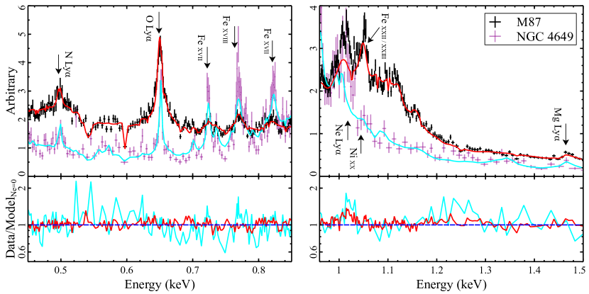
Figure 1: RGS spectra of M87 and NGC 4649 extracted from the 0–60 arcsec slice. The crosses indicate the first-order data, and the solid lines represent the best-fit models with AtomDB, but assuming Ne is 0 solar. The ratios of data to the zero-Ne models are plotted in the lower panels. The emission lines of our interesting elements are marked on the upper panels.

Table 2: Best-fitting spectral parameters for halo emission within 60 arcsec regions.

Object	$\langle kT\rangle$	$kT_{\textrm{hot}}$	VEM${}_{\textrm{hot}}$	VEM${}_{\textrm{middle}}$	VEM${}_{\textrm{cool}}$	C-stat/dof	Regime
	(keV)	(keV)	($10^{10}$ cm-5)	($10^{10}$ cm-5)	($10^{10}$ cm-5)
NGC 1404	$0.49\pm 0.08$	$0.68\pm 0.14$	$16\pm 2$	$16.9\pm 1.0$	$1.7\pm 1.0$	4441.3/3512	C
NGC 4636	$0.61\pm 0.04$	$0.77\pm 0.06$	$27.6\pm 0.7$	$14.4\pm 0.8$	$2.4\pm 0.7$	3594.8/3259	C
NGC 4649	$0.82\pm 0.04$	$0.86\pm 0.13$	$27.2^{+2.7}_{-0.7}$	$<0.7$	$1.8\pm 0.3$	3558.5/3343	C
NGC 5846	$0.56\pm 0.12$	$0.8\pm 0.2$	$20.1^{+0.5}_{-4.6}$	$13.8^{+4.3}_{-0.6}$	$4.0^{+0.4}_{-3.0}$	3468.9/3316	C
M49	$0.92\pm 0.05$	$0.98\pm 0.08$	$32.3\pm 0.9$	$3.8\pm 0.3$	$0.6\pm 0.5$	3738.9/3476	C
HCG 62	$0.80\pm 0.14$	$1.0\pm 0.3$	$26\pm 4$	$5.7\pm 1.3$	$4.3^{+9.7}_{-0.7}$	3240.8/3154	C
Fornax	$0.83^{+0.17}_{-0.04}$	$0.9^{+1.38}_{-0.06}$	$50^{+28}_{-1}$	$3.8\pm 0.4$	$3.2^{+47.1}_{-0.7}$	4196.4/3582	C
NGC 1550	$1.26\pm 0.16$	$1.3\pm 1.0$	$40^{+3}_{-22}$	$0.44^{+1.4}_{-0.2}$	$0.6\pm 0.4$	3596.5/3575	W
M87	$1.5\pm 0.2$	$1.53^{+1.1}_{-0.3}$	$4.2^{+2.2}_{-0.4}\times 10^{2}$	$16.6^{+8.7}_{-1.5}$	$1.2^{+1.0}_{-0.5}$	4122.0/3672	W
A3581	$1.56\pm 0.07$	$1.6\pm 0.2$	$95\pm 5$	$2.2\pm 0.8$	$0.7\pm 0.4$	3649.5/3589	W
A262	$1.8\pm 0.3$	$1.9\pm 0.4$	$71\pm 10$	$3.5\pm 0.5$	$1.1\pm 0.3$	3181.4/3379	W
AS 1101	$2.6\pm 0.2$	$2.6\pm 0.5$	$(1.51\pm 0.14)\times 10^{2}$	$3.1^{+3.2}_{-1.3}$	$1.2\pm 0.3$	3812.1/3659	H
AWM 7	$2.8\pm 0.5$	$2.9\pm 0.9$	$79\pm 15$	$1.3^{+4.8}_{-0.9}$	$1.5\pm 0.3$	3672.6/3644	H
Perseus	$2.73\pm 0.18$	$2.8\pm 0.4$	$(1.39\pm 0.13)\times 10^{3}$	$11^{+45}_{-4}$	$30\pm 4$	4359.0/3668	H

Note. — Column (1): Object name. Column (2): The VEM-weighted average temperature. Column (3): Temperature of the hot component. Columns (4)(5)(6): The volume emission measures (VEMs) of each temperature component. The VEM is given as $\int n_{e}n_{\textrm{H}}dV/(4\pi D^{2})$, where $V$ and $D$ are the volume of the emission region (cm³) and the angular diameter distance to the emitting source (cm), respectively. Column (7): The ratio of C-statistic values to degrees of freedom. Column (8): We define three temperature regimes of cool (C), warm (W), and hot (H): $\langle kT\rangle$ is less than 1.0 keV, greater than 1.0 keV and less than 2.0 keV, and greater than 2.0 keV, respectively.

Table 3: The Fe abundance and the N/Fe, O/Fe, Ne/Fe, Mg/Fe, and Ni/Fe ratios for halo emission within 60 arcsec regions. For NGC 4649, HCG 62, Fornax, and NGC 1550, the O/Fe, Ne/Fe, and Mg/Fe ratios are computed by averaging over each radial bin (see § 3.2).

Object	Fe	N/Fe	O/Fe	Ne/Fe	Mg/Fe	Ni/Fe
	(solar)	(solar)	(solar)	(solar)	(solar)	(solar)
NGC 1404	$0.34\pm 0.02$	$2.1\pm 0.4$	$0.58\pm 0.04$	$1.28\pm 0.14$	$1.66\pm 0.15$	$3.4\pm 0.5$
NGC 4636	$0.56\pm 0.02$	$1.6\pm 0.3$	$0.64\pm 0.04$	$0.89\pm 0.09$	$1.10\pm 0.11$	$2.4\pm 0.3$
NGC 4649	$0.39^{+0.08}_{-0.02}$	$2.6\pm 0.8$	$0.73\pm 0.09$	$1.52\pm 0.12$	$1.31\pm 0.14$	$1.7\pm 0.4$
NGC 5846	$0.35\pm 0.01$	$2.5\pm 0.5$	$0.74\pm 0.09$	$1.24\pm 0.13$	$1.33\pm 0.16$	$4.2\pm 0.6$
M49	$0.46\pm 0.03$	$2.7\pm 0.6$	$1.01\pm 0.09$	$1.45\pm 0.19$	$1.86\pm 0.16$	$2.9\pm 0.4$
HCG 62	$0.24^{+0.10}_{-0.02}$	$1.1\pm 0.8$	$1.01\pm 0.07$	$1.44\pm 0.18$	$2.2\pm 0.2$	$1.5\pm 0.7$
Fornax	$0.28\pm 0.02$	$4.3\pm 0.9$	$1.23\pm 0.09$	$1.52\pm 0.13$	$1.77\pm 0.16$	$4.8\pm 0.6$
NGC 1550	$0.57\pm 0.07$	$3.5\pm 1.3$	$1.31\pm 0.10$	$0.91\pm 0.16$	$0.61\pm 0.18$	$1.9\pm 0.5$
M87	$0.67^{+0.16}_{-0.04}$	$2.5\pm 0.4$	$1.09\pm 0.05$	$0.97\pm 0.07$	$1.02\pm 0.08$	$1.9\pm 0.2$
A3581	$0.66\pm 0.04$	$<1.3$	$1.14\pm 0.10$	$0.96\pm 0.17$	$1.15\pm 0.15$	$0.7\pm 0.3$
A262	$1.0\pm 0.2$	$3.8\pm 1.4$	$1.23\pm 0.16$	$1.1\pm 0.3$	$0.7\pm 0.3$	$1.1\pm 0.6$
AS 1101	$0.67\pm 0.09$	$<0.8$	$1.10\pm 0.10$	$0.99\pm 0.14$	$0.76\pm 0.15$	$1.0\pm 0.4$
AWM 7	$2.0^{+1.4}_{-0.4}$	$<0.4$	$1.17\pm 0.09$	$0.8\pm 0.2$	$1.33\pm 0.17$	$1.3\pm 0.3$
Perseus	$0.84\pm 0.06$	$0.9\pm 0.5$	$1.58\pm 0.05$	$1.14\pm 0.07$	$0.73\pm 0.05$	$1.02\pm 0.13$

The spectral fittings of the RGS X-ray spectra globally follow the same strategy of Fukushima et al. (2022a). We use xspec package version 12.10.1f (Arnaud, 1996). In the following spectral analysis, all spectra are fitted using the C-statistics (Cash, 1979) to estimate the model parameters and their error range without bias (Kaastra, 2017). The spectra are re-binned to have a minimum of one count per spectral bin. We jointly fit the first- and second-order spectra in the $0.45$–$1.75$ keV and $0.8$–$0.75$ keV bands, respectively, with the same parameters. Given that the halo emission is dominant in our analyzing regions compared to the other astrophysical background emissions, the possible instrumental component is taken into account by a steep power-law model. We take the spectral broadening effect due to the spatial extent of the source into account by using the rgsxsrc model with MOS1 images.

We use the latest AtomDB version 3.0.9 to model emissions from collisional ionization equilibrium (CIE) plasmas. The spectra of each object are modeled with triple bvvtapec components. Two temperatures for line and continuum have the same value because the continuum temperature is poorly constrained for the RGS spectra. Although the double components model has been used to reproduce halo emissions (e.g., Panagoulia et al., 2013; de Plaa et al., 2017; Lakhchaura et al., 2019; Simionescu et al., 2019), it can still underestimate the Fe abundance in some systems (the “double Fe bias”, see Mernier et al. 2022). Here, the triple components model is used in our analysis. We do not adopt any assumption regarding the emission measures of each temperature component. Instead, temperatures for each component are coupled along a geometric series with a common ratio of 0.5 to reproduce the temperature structure as $kT_{\textrm{hot}}:kT_{\textrm{middle}}:kT_{\textrm{cool}}=1:0.5:0.25$. We note that an additional fourth component does not change fitting results nor improve the fitting significantly, same as the Centaurus cluster in Fukushima et al. (2022a). The model with free temperatures also makes little change to other parameters. Our modeling interpolates the continuous temperature distribution in halos sufficiently, giving better fits than a Gaussian differential emission measure model. All three CIE plasmas are modified by a common Galactic absorption of phabs whose column densities are calculated following the method of Willingale et al. (2013) for each object (summarized in Table 1). We adopt absorption cross sections of Verner et al. (1996).

Here, we show the representative spectra derived from the 60 arcsec cores of M87 and NGC 4649 (Figure 1). Prominent K-shell emission lines of N, O, Ne, and Mg, L-shell emission lines of Fe are clearly detected in the spectra. In addition to these elements, the Ni abundance is also allowed to vary, and the abundances of other elements whose emission lines are shrouded under the continuum emission are fixed to the solar value. All abundances for three temperature components are tied together. Finally, we allow the volume emission measures (VEMs) of each component to vary, which is given as $\int n_{e}n_{\textrm{H}}dV/(4\pi D^{2})$, where $n_{e}$ and $n_{\textrm{H}}$ are electron and proton density, $V$ and $D$ are the volume of the emission region and the angular diameter distance to the object, respectively.

We perform the fitting to spectra extracted not only from each slice with 0–6, 6–18, 18–60, and 60–120, and 0–60 arcsec. Our modeling largely gives a good fit with the ratios of the C-statistic value to degrees of freedom (C-stat/dof) $\sim 1$ in the broader region as well as each slice. The fitting results are summarized in Tables 2 and 3 for the 0–60 arcsec regions. Results for each slice will be indicated in figures in subsequent sections. In Figure 1, the model partially fails to reproduce the spectrum of NGC 4649 around the 0.7–0.8 keV band, wherein the Fe xvii and Fe xviii lines are affected by a large optical depth of resonant scattering (e.g., Sanders et al., 2008; Ogorzalek et al., 2017). Mernier et al. (2022) suggests that fearlessly excluding the Fe xvii line makes marginal changes in the abundance ratios less than 10 percent. In addition, we also test to add Gaussians with a negative normalization at these emission lines to avoid the resonant scattering effect in some early-type galaxies. However, this model does not significantly change our measurement of abundance ratios. It can matter just on reproducing line intensities of Fe, especially for Fe xvii and Fe xviii, not on measuring abundances and ratios.

3.2 Radial abundance profiles

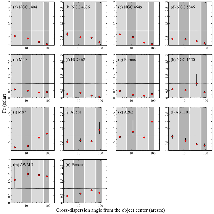
Figure 2: Radial profiles of the Fe abundance as a function of radial distance in units of arcseconds from the center of each object. Grey areas show the width of the slice region for RGS analysis: 0–6, 6–18, 18–60, and 60–120 arcsec from left to right, respectively. The solar ratio is indicated with dotted lines on each panel.

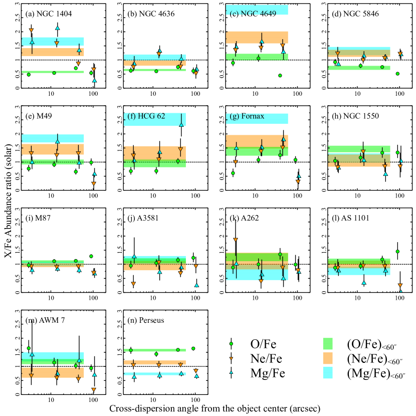
Figure 3: Radial profiles of the O/Fe, Ne/Fe, Mg/Fe abundance ratios for each object. The circles, down-, and up-triangles represent the O/Fe, Ne/Fe, and Mg/Fe ratios, respectively, as a function of distance in units of arcseconds from the center of each object. The plots are slightly shifted on the $x$-axis for clarity. Color-shaded areas show the ratios obtained from broad 60 arcsec slices. The solar ratio is indicated with dotted lines on each panel.

Here, we show the central metal distribution in the hot halos of each system. In Figure 2, radial profiles of the Fe abundance are plotted for each object. In some previous works with CCD detectors, NGC 4636, NGC 4649, NGC 5846, HCG 62, A3581, A262, AS 1101, and Perseus are proposed to show an Fe abundance drop (e.g., Churazov et al., 2003; Panagoulia et al., 2015; Liu et al., 2019). Our RGS results show no clear abundance declination in these objects, excluding a hint of drop for the Perseus cluster. M87 shows a sharp Fe drop, where no abundance drop has been reported with CCD studies to date (e.g., Matsushita et al., 2003; Million et al., 2011; Gatuzz et al., 2023). However, we should be cautious in interpreting these profiles because the metal abundances are estimated with the RGS instrument. Additionally, the abundance drop might be detected only with broadband spectra, including both the Fe L- and K-shell emission lines (Gatuzz et al., 2022, for the Centaurus cluster).

The relative abundance ratio to Fe is a more robust parameter than the absolute abundance in the RGS analysis (e.g., de Plaa et al., 2017; Gastaldello et al., 2021). We plot the O/Fe, Ne/Fe, and Mg/Fe abundance ratios in Figure 3, discarding the outermost bins of NGC 4649 and HCG 62 with large errors ($>$ 1.5 solar) due to their line-poor or line-less spectra. This is the first report of the Ne distribution using the RGS data sets. Given that the Ne-Ly$\alpha$ lines are completely shrouded in the Fe-L bump with CCD spectra, our Ne profile is possibly more reliable than previous ones (e.g., Million et al., 2011; Liu et al., 2019). More importantly, such a flat distribution has no individuality among the samples, whether or not an object shows the abundance drop (in CCD spectra, e.g., Panagoulia et al. 2013; Liu et al. 2019). The ratios are largely around the solar ratio and give a flat profile within the 60 arcsec regions in each object but for NGC 1404. In NGC 1404, the Ne/Fe and Mg/Fe ratios exhibit clear central enhancements despite a flat distribution of O/Fe like the other systems. Following Mernier et al. (2022), we also took the halo emission from the Fornax cluster into account as a background in the outer two bins. Our background estimation does not change the abundance measurements in the outer region of NGC 1404.

3.3 Abundances and temperature in the central 60 arcsec

As reported in § 3.2, the O/Fe, Ne/Fe, and Mg/Fe profiles generally show a flat distribution in the central 60 arcsec core of each halo, suggesting that the metal content is remarkably uniform in the central cores. The best-fit parameters for the 0–60 arcsec slice are summarized in Tables 2, 3, and Figure 3 (shaded areas). It is noteworthy that our estimated abundance ratios for the Perseus cluster are globally consistent with the previous work by Simionescu et al. (2019) despite a different fitting strategy. The lower Fe abundance of theirs ($\sim 0.4$ solar) mainly originates from a narrower width of about 0.8 arcmin than ours and/or simple two-temperature components modeling.

In Table 2, we also give the VEM-weighted average temperatures (denoted as $\langle kT\rangle$) derived within 60 arcsec. These values suggest that our samples seem to be divided into three subgroups by $\langle kT\rangle$ of halos. Henceforward, two threshold temperatures ($\langle kT\rangle$ $=$ 1 and 2 keV) determine three regimes of cool, warm, and hot halos (denoted by C, W, and H, respectively). Tables 1 and 2 suggest that three temperature regimes correspond well to the traditional object classification, i.e., “galaxies”, “groups”, and “clusters”.

One caveat is that the abundance ratios derived from the cumulative spectra are sometimes overestimated, especially for Mg/Fe, compared to those of each individual bin (e.g., see the cyan area and up-triangles for NGC 4649, Figure 3(c)). Such a schism is seen in the C-regime objects that have relatively low Mg lines (Figure 1(b)). Abundance estimation by RGS is hard for elements whose emission lines do not dominate the continuum (e.g., de Plaa et al., 2017; Mao et al., 2019; Gastaldello et al., 2021). A strategy of narrow-band fits at $1.3$–$1.6$ keV around the Mg Ly$\alpha$ line, which can minimize such biases, improves overestimation, yielding Mg/Fe $=$ 1.5, 2.1, and 2.2 solar for NGC 4649, HCG 62, and Fornax, respectively. Thus, despite better photon statistics of cumulative spectra, we report in Table 3 and adopt in subsequent sections the average ratios over the inner three bins instead of unnaturally high ratios for concerning objects.

3.4 AtomDB vs SPEXACT

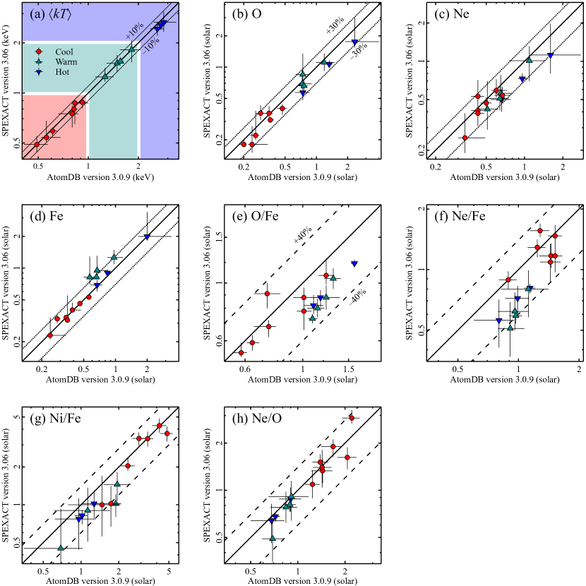
Figure 4: Comparisons of the spectral parameters obtained from central 60 arcsec slices for each object when using AtomDB or SPEXACT. (a) The VEM-weighted averaged halo temperature. Our sample is subdivided into three subsamples: cool, warm, and hot (see the text) plotted by the circles, up-, and down-triangles, respectively. (b, c, d) The absolute abundances of O, Ne, and Fe. (e, f, g, h) The relative abundance ratios of O/Fe, Ne/Fe, Ni/Fe, and Ne/O. The solid lines in each panel indicate equal values between the two codes. The thin-solid, dotted, and dashed lines delimitate $\pm$10, 30, and 40 percent limits, respectively.

Abundance measurements suffer from a systematic bias caused by atomic code uncertainties (e.g., Mernier et al., 2020, for a review). In this work, we test the SPEXACT version 3.06 (Kaastra et al., 1996) for the spectra extracted within 60 arcsec regions to study the uncertainties arising from systematics in the atomic data. In order to minimize modest deviations in the modeling procedure of xspec and spex, we tabulate the lines and continuum calculated by a simple cie model at 201 bins of temperature on spex and export them into APEC table format that can be read in xspec. This process is done with a python code .

In Figure 4, we show direct comparisons of $\langle kT\rangle$, abundances, and relative abundance ratios between AtomDB and SPEXACT. Clearly seen is that the $\langle kT\rangle$ measurements are in quite good agreements between the two codes ($\lesssim$ 10 percent) irrespective of halo temperature regimes (Figure 4(a)). Such agreements on gas temperature between two codes have also been reported not only for RGS data but also for calorimetric ones (Hitomi Collaboration et al., 2018; Simionescu et al., 2019). The O, Ne, and Fe abundances are largely consistent with each other in up to $\sim$ 30 percent differences. For the abundance ratios, more moderate agreements $\lesssim$ 40 percent are measured (Figures 4(e), (f), (g), and (h)). The Ne/O ratios show a relatively small scatter compared to O/Fe, Ne/Fe, and Ni/Fe, and are consistent within error ranges. These differences between the two codes are possibly consistent with the report of the abundance measurements in the intracluster medium (Mernier et al., 2020). The most important is that these agreements between the atomic codes are independent of the temperature regimes.

4 Discussion

4.1 Flat O/Fe, Ne/Fe, and Ne/O profiles

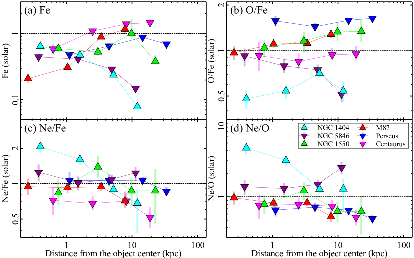
Figure 5: Radial profiles of (a) Fe, (b) O/Fe, (c) Ne/Fe, and (d) Ne/O for representative objects. All are plotted as a function of distance in units of kiloparsecs from the center of each system. No Fe abundance drop has been reported in objects plotted by up-triangles, and down-triangles are for the Fe drop ones. The values of the Centaurus cluster are retrieved from Fukushima et al. (2022a). The solar ratio is indicated with dotted lines on each panel.

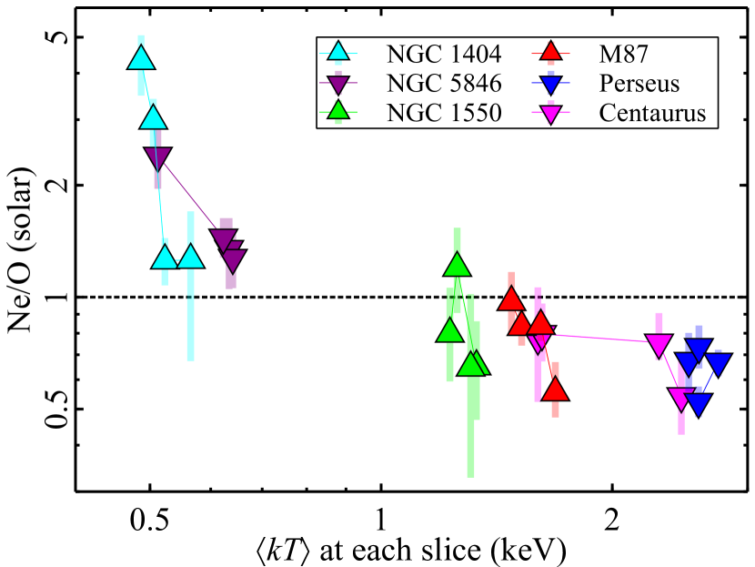
Figure 6: The Ne/O ratio plotted against local $\langle kT\rangle$ at each slice for the same objects of Figure 5. The solar ratio is indicated with dotted lines on each panel.

As described in Section 1, the mechanisms of the abundance depletions are still elusive. Panagoulia et al. (2015) and Lakhchaura et al. (2019) proposed the dust grains origin for such abundance drop and noted that the distribution of non-reactive elements (Ne and Ar) is important to inspect this picture. For the Centaurus cluster, Fukushima et al. (2022a) reported flat radial profiles of the Ne/Fe and Ar/Fe ratios, which suggests that Fe and non-reactive elements have the same spatial distribution. This result is difficult to explain only by the dust origin process.

In Figures 5, we show the (a) Fe, (b) O/Fe, (c) Ne/Fe, and (d) Ne/O profiles for representative objects in addition to our previous results of the Centaurus cluster. While the Fe abundance shows various profiles among the objects, the O/Fe, Ne/Fe, and Ne/O abundance ratios are relatively flat in the central two or three bins, except for NGC 1404. For the majority of our samples, noble gas Ne and other metals identically distribute in halos regardless of the (possible) presence of an abundance drop. While O and Fe are independently synthesized by CCSNe and SNeIa, respectively, the dominance of O and Ne must share the same origin. Thus, flat Ne/Fe and Ne/O profiles strongly contradict the dust grains scenario. Additionally, measuring the absolute abundance with the RGS spectra suffers from systematic uncertainties since the grating spectra are dominated by line emissions rather than continuum emissions (e.g., Mernier et al., 2018a). Hence, the Fe abundance drop suggested for M87 and Perseus is caused at least partly by other physical processes and/or uncertainties in abundance measurement like atomic codes.

One exception is a clear enhancement of Ne with respect to O and Fe for NGC 1404 (Figures 5(c) and (d)). However, Mernier et al. (2022) determined the abundance distribution of Mg, Si, and Fe by CCDs on board XMM-Newton, where the centrally-peaked profiles rather than dropping ones are reported, especially for Fe. Our increasing profiles of Fe and Mg/Fe toward the center support their results (see Figures 2(a) and 3(a)). Additionally, if dust grains do work significantly in this object, common increases of Ne/Fe and Mg/Fe are unreasonable because Mg is easily depleted into dust compared to noble-gas Ne. The dust formation scenario likely does not matter in NGC 1404 even if an increasing Ne/O profile is observed.

Worth mentioning is that the innermost $\langle kT\rangle$ of NGC 1404 is the coolest one in our analysis (§3.1). Here, we also plot the Ne/O ratios as a function of local $\langle kT\rangle$ at each slice (Figure 6). Interestingly, high Ne/O ratios are observed at lower temperature slices in one object, as well as for cooler systems among the sample. The possible correlation of Ne/O to $\langle kT\rangle$ suggests some uncertainties in the abundance estimation of cool plasmas. This will be discussed in more detail in § 4.2.2.

4.2 Metal composition, $\langle kT\rangle$ and $M_{<60^{\prime\prime}}/L_{B}$

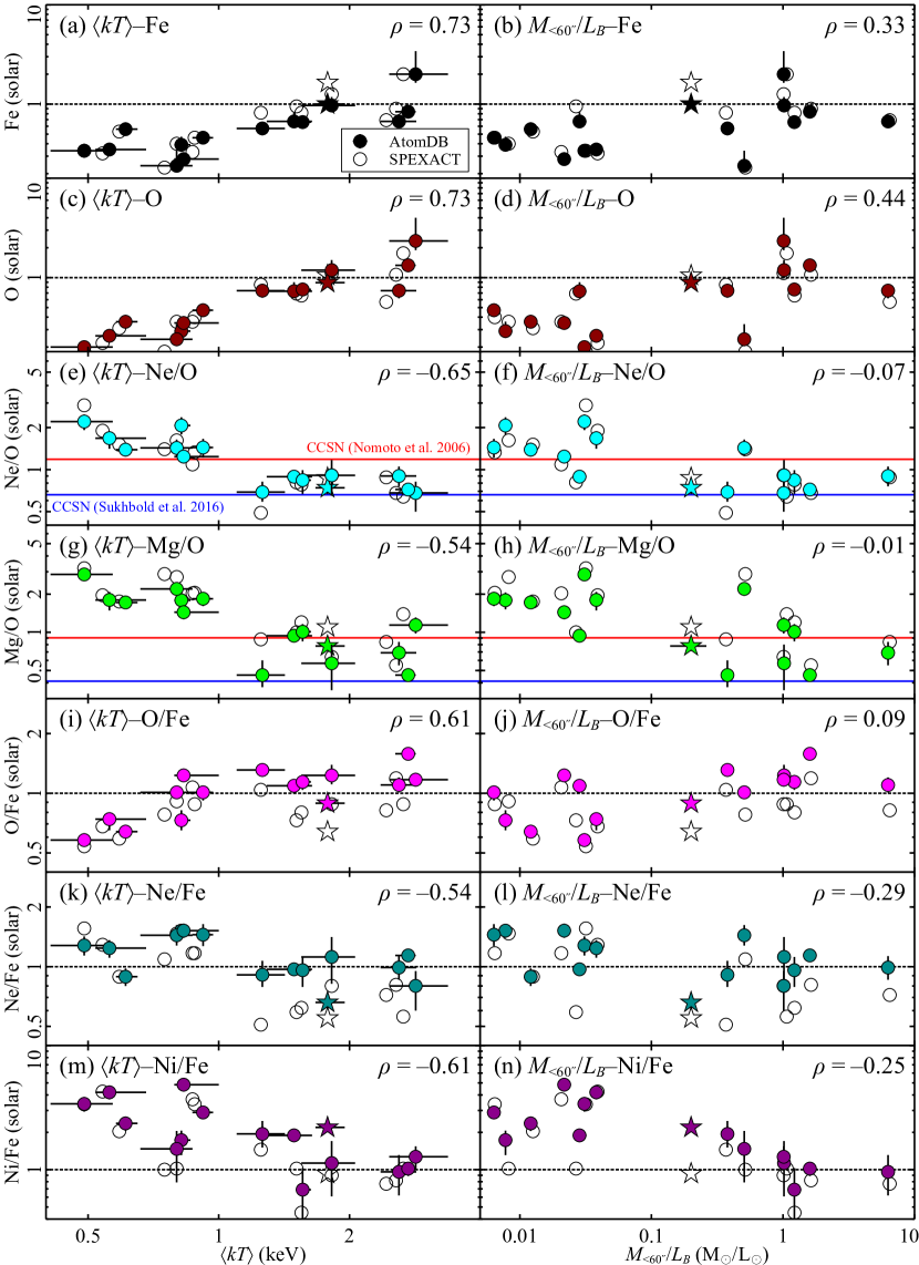
Figure 7: The Fe and O abundances and the Ne/O, Mg/O, O/Fe, Ne/Fe, and Ni/Fe ratios as functions of (a, c, e, g, i, k, m) $\langle kT\rangle$ and (b, d, f, h, j, l, n) $M_{<60^{\prime\prime}}/L_{B}$, respectively. The filled and open circles represent the results with AtomDB and SPEXACT, respectively. The stars indicate the results of Centaurus (Fukushima et al., 2022a). Errors are shown only for the AtomDB results for viewing purposes. We also show expected ratios by two major CCSN nucleosynthesis models (Nomoto et al., 2006; Sukhbold et al., 2016) on the Ne/O and Mg/O panels. The Pearson’s correlation coefficients with the AtomDB results are shown at the right-top corners on each panel.

Here, we show trends in the metal content of various halos in our sample. One of the most common indicators characterizing the gas property is of course $\langle kT\rangle$; moreover, integrated mass-to-light ratio can be another diagnostic of halos (e.g., Nagino & Matsushita, 2009). We computed the mass parameter by integrating the electron density in the 60 arcsec slices with a rough assumption that the emission is from a uniform-density sphere. Although this is not identical to the true halo mass, such a pseudo-mass parameter (denoted by $M_{<60^{\prime\prime}}$) is a good surrogate for the gas mass at the central part where the halo emission is dominant. By using parameters of the Centaurus cluster, Fukushima et al. (2022a) showed that the $M_{<60^{\prime\prime}}$ calculated from the RGS is in plausible agreement ($\sim 30$ percent) with the more accurate mass estimated by integrating the VEM profile from CCDs. Then, we adopt the $B$-band luminosity (denoted with $L_{B}$) listed in Table 1 to calculate the mass-to-light ratio. In Figure 7, we plot the abundances and abundance ratios as functions of $\langle kT\rangle$ and $M_{<60^{\prime\prime}}/L_{B}$.

4.2.1 Absolute abundance

A general trend is that the absolute abundances show a positive correlation to $\langle kT\rangle$ with the Pearson’s correlation coefficients $\sim 0.7$ (Figures 7(a) and (c)). While the abundance distribution for $M_{<60^{\prime\prime}}/L_{B}$ has a relatively large scatter, most of the low metallicity systems are located at the low $M_{<60^{\prime\prime}}/L_{B}$ regime (Figures 7(b) and (d)). Considering ongoing SNIa enrichments in low-$M_{<60^{\prime\prime}}/L_{B}$ objects, it is unreasonable that these systems show lower Fe abundance than the high $M_{<60^{\prime\prime}}/L_{B}$ systems possibly contributed by primordial gas. Similarly, the lowest O abundances for the coolest objects (Figures 7(c) and (d)) indicates that the C regime objects (globally identical to the low-$M_{<60^{\prime\prime}}/L_{B}$ ones) are less enriched with O, which is hard to interpret due to present metal supplies by mass loss.

Importantly, absolute abundances with RGS spectra are suffered from continuum estimation, especially for subkiloelectronvolt plasmas. The systematics in such cool plasmas have also been pointed out by many authors (e.g., Matsushita et al., 1997, 2000; Gastaldello et al., 2021; Fukushima et al., 2022a). Even the CCD spectra are contaminated by continuum emissions from two-photon and free-bound processes by heavy metals in cool plasmas; therefore, absolute abundance measurements in the C or low-$M_{<60^{\prime\prime}}/L_{B}$ regimes are challenging with the RGS spectra that are dominated by line emissions. We suspect that this possible bias in the C regime intrinsically contributes to the observed abundance drops in the central coolest part of a system.

4.2.2 Ne/O and Mg/O

We also plot the Ne/O and Mg/O ratios that are dominantly expelled via mass-loss winds and CCSNe, and thus, represent nucleosynthesis in a core of supergiants. There are clear interrelations for $\langle kT\rangle$–Ne/O and $\langle kT\rangle$–Mg/O; as those at the C regime are higher than the solar ratios that are uniformly observed at the W+H regime (Figures 7(e) and (g)). In Figures 7(f) and (h), there are no clear correlations to $M_{<60^{\prime\prime}}/L_{B}$ with virtually zero Pearson’s correlation coefficients compared to relations to $\langle kT\rangle$. However, it is an enigmatic picture that O, Ne, and Mg patterns of early-type galaxies contributed by stellar populations are completely different from the ones in the medium in groups and clusters. For example, the Fornax cluster and NGC 1404 are a host and its member galaxy, respectively, that belong to the same regimes and have similar patterns. The Virgo cluster hosts NGC 4649, M49, and M87, the former two of which exhibit the super-solar Ne/O and Mg/O ratios.

Given that O and Ne share dominantly the same origin and enrichment process, such schisms are hard to explain by a physical process. Unless a picture of the dust-depleted process recovers validity after a decrease of the conflict with flat Ne/O profiles (Figure 5), the abundance measurement uncertainty is instead a natural solution at present. As both AtomDB and SPEXACT give consistent ratios, this possible uncertainty depends on $\langle kT\rangle$. Different from the strong O Ly$\alpha$ line, the Ne Ly$\alpha$ and/or Ne He$\alpha$ lines are not resolved completely from the Fe L bump even with RGS (Figure 1); and hence, the Ne/O ratios of the coolest objects likely suffer from some systematics. If this is the case, unreasonably high Ne/O ratios at the center of NGC 1404 (Figure 5(d)), which is the coolest object in our sample, are naturally interpreted as upward-biased values. In addition, the Mg/O ratio, uniformly high in the C regime, is also difficult to measure due to the low relative intensity of Mg lines in subkiloelectronvolt plasmas.

4.2.3 O/Fe and Ne/Fe

Generally, abundance ratios concerning Fe show a correlation to $\langle kT\rangle$, and have a rather weak relation with $M_{<60^{\prime\prime}}/L_{B}$ (Figures 7(i), (j), (k), and (l)). In previous studies, uniform abundance and ratios among objects in the wide mass range are reported (e.g., de Plaa et al., 2007; Mernier et al., 2018b). In Figure 7(i), the O/Fe ratio does not correlate significantly to $\langle kT\rangle$ excluding the coolest objects, which is consistent with de Plaa et al. (2017). While de Plaa et al. (2017) reported that the O/Fe ratio does not vary depending on gas temperature, including subkiloelectronvolt objects, recent works with the latest atomic codes give lower O/Fe ratios than those measured by them (e.g., Mernier et al., 2022). The lower O/Fe of cool objects, which is possibly a biased value, is preferable under the latest codes.

Figure 7(k) is the first robust result of the $\langle kT\rangle$–Ne/Fe relation. The Ne/Fe ratios have a negative $\langle kT\rangle$ correlation with $\sim-0.5$ coefficient and give a clear delimitation of $\langle kT\rangle$ $=1$ keV while Figure 7(l) shows that the correlation between Ne/Fe and $M_{<60^{\prime\prime}}/L_{B}$ is more marginal with the Pearson’s coefficient $\sim-0.3$. We found a hint of anti-correlation of Ne/Fe to $\langle kT\rangle$ different from the $\langle kT\rangle$–O/Fe relation, which is also suggested in Figure 7(e). As well as the Ne/O ratios, these inverse properties of O and Ne to each other are unreasonable because of their same origin and dispersal history.

4.2.4 Ni/Fe

The Ni/Fe ratios show a moderate negative correlation to both $\langle kT\rangle$ and $M_{<60^{\prime\prime}}/L_{B}$ (Figures 7(m) and (n)). When objects fall on the $M_{<60^{\prime\prime}}/L_{B}\gtrsim 1\,\textrm{M}_{\odot}/\textrm{L}_{\odot}$ region, the Ni/Fe ratios are consistent with the solar ratio. The low-$M_{<60^{\prime\prime}}/L_{B}$ objects with $M_{<60^{\prime\prime}}/L_{B}\lesssim 0.1\,\textrm{M}_{\odot}/\textrm{L}_{\odot}$ exhibit high Ni/Fe ratios larger than 2 solar. While we are now prevented from assessing the Ni/Fe ratio robustly by the absence of prominent lines of Ni in the RGS band (Figure 1), a high Ni/Fe ratio is also reported with CCD for the Centaurus cluster (Fukushima et al., 2022a). As indicated in many previous works, the Ni/Fe ratio is sensitive to SNIa explosion models since a dominant fraction of Ni is synthesized at a core of exploding white dwarves (e.g., Dupke & White, 2000; de Plaa et al., 2007; Hitomi Collaboration et al., 2017; Mernier et al., 2017). This will be discussed more in detail at § 4.3.

4.2.5 N enrichment

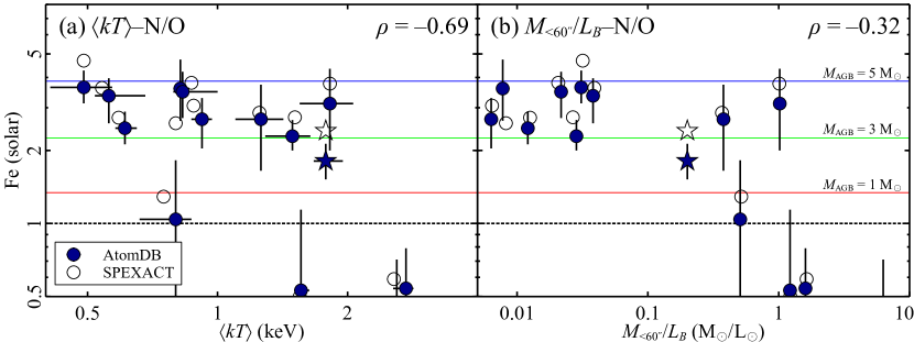
Figure 8: The N/O ratios as functions of (a) $\langle kT\rangle$ and (b) $M_{<60^{\prime\prime}}/L_{B}$. The filled and open circles represent the results with AtomDB and SPEXACT, respectively. The stars indicate the results of Centaurus (Fukushima et al., 2022a). Errors are shown only for the AtomDB results for viewing purposes. The predicted ratios by Karakas (2010) are shown by horizontal solid lines, assuming the initial metallicity of AGBs at each mass to the solar value. The Pearson’s correlation coefficients for the AtomDB results are given at the right-top corners on each panel.

The N enrichment through SNe is negligible, and they can be instead produced and expelled by AGB stars. We plot the N/O ratios of each object against $\langle kT\rangle$ and $M_{<60^{\prime\prime}}/L_{B}$ (Figures 8(a) and (b)), comparing them to the model prediction in mass-loss winds from AGBs ($M_{\textrm{initial}}$ = 1, 3, 5$\textrm{M}_{\odot}$, Karakas 2010). The N/O ratios are uniformly over-solar $\sim$ 2–4 solar among various objects, which are well explained by enrichments via AGBs $\lesssim 5$ $\textrm{M}_{\odot}$. Here, the dominant fraction of observed N and O is expected to be from AGB stars that should be an ongoing enrichment channel in central regions of early-type galaxies. Since a contribution from early CCSNe to the O enrichment is undoubtedly important in accumulated halo history, the direct comparison of observed N/O and AGB yields is simplistic and cannot fully rule out a possible effect of more massive AGB stars. However, Mao et al. (2019) pointed out the importance of the contribution of low- and intermediate-mass stars ($\sim$ 0.9–7 $\textrm{M}_{\odot}$) in AGB to the halo enrichment. Additionally, Kobayashi et al. (2020) also attributed the N enrichment in the Milky Way to inter-mediate mass AGBs (4–7 $\textrm{M}_{\odot}$). Even our simple estimation gives a globally consistent result with these works.

Some hot or high-$M_{<60^{\prime\prime}}/L_{B}$ objects (giant clusters like Perseus) yield N/O $\lesssim 1$ solar, unlike the global trend of high N/O ratios. One possibility is that mass-loss contribution is strong in the cool or low $M_{<60^{\prime\prime}}/L_{B}$ halos compared to high N/O objects. However, the N Ly$\alpha$ line is weak in hot gas ($\gtrsim 2$ keV) and measuring the N abundance in the hot halos is harder than in the cool ones (Mao et al., 2019). Therefore, retrieving relations around the hot or high-$M_{<60^{\prime\prime}}/L_{B}$ regimes from Figure 8 is somewhat cautious. A more precise trend of N/O will be validated by comparing simulation studies with realistic assumptions of various initial mass functions (IMFs) and mass injection rates. Spatially-resolved analysis with non-dispersive instruments will also provide a unique way to investigate the N enrichment in early-type galaxies.

4.3 Entire abundance patterns and SN yields

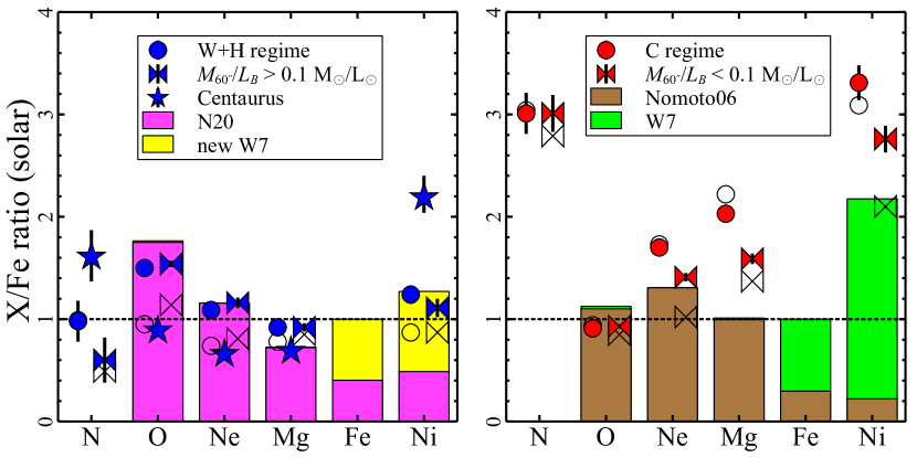
Figure 9: Abundance ratio patterns obtained in central 60 arcsec cores. The sample is divided into two subsamples using temperature regimes (circles) and $M_{<60^{\prime\prime}}/L_{B}=0.1\,\textrm{M}_{\odot}/\textrm{L}_{\odot}$ (ties), each of which the abundance ratios are averaged. The stars represent the result of the Centaurus cluster given in Fukushima et al. (2022a). Filled and open plots indicate the results of AtomDB and SPEXACT, respectively. To fit the observed pattern, we adopt two combination models of CCSN and SNIa yields: the “classical” CCSN model (Nomoto et al., 2006) and W7 model (Iwamoto et al., 1999), and N20 model (Sukhbold et al., 2016) and new W7 model (Leung & Nomoto, 2018). Every progenitor metallicity thereof is assumed to be 1 solar. For viewing purpose, only two combination with the best $\chi^{2}$/dof are presented for $M_{<60^{\prime\prime}}/L_{B}$ subsamples with AtomDB. See Table 5 for the results of other regimes and combination.

Table 4: Error-weighted average abundance ratios to Fe with AtomDB for each subsample. Statistical variances are also given in parentheses.

	C	W+H	low-$M_{<60^{\prime\prime}}/L_{B}$	high-$M_{<60^{\prime\prime}}/L_{B}$
N/Fe	$3.0\pm 0.2$ (1.3)	$1.0\pm 0.2$ (2.7)	$3.01\pm 0.18$ (0.59)	$0.6\pm 0.2$ (2.9)
O/Fe	$0.91\pm 0.02$ (0.05)	$1.50\pm 0.02$ (0.10)	$0.93\pm 0.02$ (0.06)	$1.54\pm 0.03$ (0.13)
Ne/Fe	$1.70\pm 0.06$ (0.18)	$1.09\pm 0.04$ (0.02)	$1.41\pm 0.04$ (0.06)	$1.16\pm 0.05$ (0.05)
Mg/Fe	$2.03\pm 0.06$ (0.30)	$0.92\pm 0.04$ (0.06)	$1.59\pm 0.05$ (0.11)	$0.92\pm 0.04$ (0.30)
Ni/Fe	$3.31\pm 0.17$ (1.44)	$1.24\pm 0.09$ (0.19)	$2.76\pm 0.13$ (1.39)	$1.11\pm 0.09$ (0.15)

Table 5: Number ratio of SNeIa to total SNe at the best-fit combination models for each regime using the AtomDB results.

	C	W+H	low-$M_{<60^{\prime\prime}}/L_{B}$	high-$M_{<60^{\prime\prime}}/L_{B}$
W7 (Iwamoto et al., 1999) + “classical” (Nomoto et al., 2006)
SNIa/(SNIa+CCSN)	$0.18\pm 0.05$	$0.18\pm 0.05$	$0.19\pm 0.04$	$0.16\pm 0.05$
$\chi^{2}$/dof	11.5/3	15.4/3	5.6/3	20.9/3
new W7 (Leung & Nomoto, 2018) + N20 (Sukhbold et al., 2016)
SNIa/(SNIa+CCSN)	$0.18\pm 0.09$	$0.11\pm 0.02$	$0.17\pm 0.08$	$0.11\pm 0.02$
$\chi^{2}$/dof	32.4/3	1.9/3	25.4/3	2.0/3

In order to summarize the entire trend of metal content for our sample, we calculate the error-weighted average X/Fe ratios for four subsamples of C, W+H, low-, and high-$M_{<60^{\prime\prime}}/L_{B}$ (Table 4). We also show the X/Fe patterns and the best-fit linear combinations of current SN yield models (Figure 9 and Table 5). In the left-hand panel of Figure 9, the ratios are plotted for the objects belonging to the W+H and high-$M_{<60^{\prime\prime}}/L_{B}$ regimes. The average ratios for the C and low-$M_{<60^{\prime\prime}}/L_{B}$ objects are shown in the right-hand panel. The result of Centaurus of Fukushima et al. (2022a) is not included in averages in the left-hand panel.

We reproduce these patterns with a linear combination model of various CCSN and SNIa nucleosynthesis calculations (e.g., Simionescu et al., 2019). Since the important ratio of SNIa to all SNe is commonly 10–20 percent with each combination, we here give representative results with the latest calculations of N20 model from Sukhbold et al. (2016) $+$ new W7 model of Leung & Nomoto (2018). The results with well-established “classical” yields of Nomoto et al. (2006) $+$ W7 model of Iwamoto et al. (1999) are also reported for comparison. The IMF of Salpeter (1955) is used to average over various progenitor masses for CCSNe. We exclude yield calculations for SNeIa with a sub-Chandrasekhar mass white dwarf because specific elements to them like Ca or Cr are completely absent from patterns in Figure 9.

The N/Fe ratios are also plotted in Figure 9 for referential results. One can include AGB contribution in the combination model to reproduce the N abundance. However, the N enrichment by SN explosions is negligible, and other elements used in Figure 9 are little affected by this additional component (Mao et al., 2019). Moreover, the SN yield fitting method abandons information about timing evolution, making it difficult to separate each SN contribution from the AGB yield as the ejecta of early CCSN and SNIa had formed stars that are now in the AGB. Therefore, the N/Fe ratios are not used to fit the patterns in this study.

4.3.1 Hot or High-$M_{<60^{\prime\prime}}/L_{B}$ objects

In the left-hand panel of Figure 9, both patterns of the W+H and high-$M_{<60^{\prime\prime}}/L_{B}$ regimes are in plausible agreement for O/Fe, Ne/Fe, Mg/Fe, and Ni/Fe. The O/Fe, Ne/Fe, and Mg/Fe ratios are close to the solar ratios. This pattern is reproduced well by the latest N20 model of Sukhbold et al. (2016), also suggested in the Ne/O and Mg/O plots (Figures 7(e) and (g)). We found that the Ni/Fe ratio is also about 1 solar, especially for SPEXACT, and that it prefers the new W7 calculation by Leung & Nomoto (2018). The sub-solar N/Fe ratio of high-$M_{<60^{\prime\prime}}/L_{B}$ objects compared to the W+H ones, still cautious to directly accept (see §4.2.5), implies the SNIa effect in systems with long-timescale enrichment. Such a trend is also predicted by simulation study (e.g., Kobayashi et al., 2020). For these patterns, the number ratio of SNeIa to total SNe is $\sim 11$ percent (Table 5), which contributes to 60 percent of observed Fe. These results are globally consistent with the results for the Perseus cluster (Simionescu et al., 2019). While the two codes give consistent results within atomic code uncertainties (see §3.4), the O/Fe ratio with SPEXACT is closer to the solar value than AtomDB, which is also indicated in Simionescu et al. (2019).

Notably, the O/Fe, Ne/Fe, and Mg/Fe ratios of Centaurus are slightly smaller than the other objects in the same regime. Fukushima et al. (2022a) suggests a significant contribution of SNIa in this object compared to other cool-core systems. High N/Fe and Ni/Fe ratios also distinguish the Centaurus cluster from the others. This object likely shows an intermediate property of enrichment channels between the two temperature regimes (e.g., mass-loss winds, SNe, primordial gas), also implied by medium $\langle kT\rangle$ and $M_{<60^{\prime\prime}}/L_{B}$ in our sample (Figure 7). Interestingly, a recent cosmological simulation predicts sub-solar ratios for O/Fe, Ne/Fe, and Mg/Fe (Fukushima et al., 2022b), which is consistent with the pattern of Centaurus. While there can still be some uncertain factors in the simulation (e.g., the delay time distribution of SNIa, mass-loss rate, IMF), traditional linear combination modeling is too simplistic for discussing halo enrichment. Closer cooperative studies of observing, simulating, and theoretical modeling are more important in the next era of high-resolution spectroscopy.

4.3.2 Cool or Low-$M_{<60^{\prime\prime}}/L_{B}$ objects

It is easy to find that the C or low-$M_{<60^{\prime\prime}}/L_{B}$ regime shows the solar O/Fe ratio with both AtomDB and SPEXACT (right-hand panel of Figure 9), which makes these objects prefer the “classical” CCSN model of Nomoto et al. (2006). On the other hand, the Ne/Fe and Mg/Fe ratios are globally higher than the O/Fe, especially with AtomDB. This is also implied in the plots of Ne/O and Mg/O (Figure 7(e), (f), (g), and (h)). High Ne/Fe and Mg/Fe ratios are not reproduced well by our SN combination models with high $\chi^{2}$/dof (Table 5). In particular, the combination of the latest SN models (Sukhbold et al., 2016; Leung & Nomoto, 2018) for the C regime yield the worst $\chi^{2}$/dof value among all trials (Table 5). The Ni/Fe ratios are higher than 2 solar, sometimes exceeding the high predictive value of the W7 model by Iwamoto et al. (1999). Super-solar N/Fe ratios are well explained by mass-loss winds from 3–4$\textrm{M}_{\odot}$ stars in AGB, consistent with the picture provided in § 4.2.5. The best-fit combination model suggests that SNIa/SN is $\sim 20$ percent (Table 5) and SNeIa produce 70 percent of Fe.

4.4 Future prospects

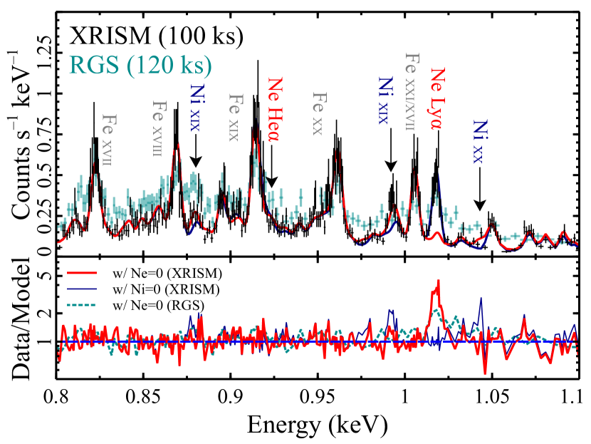
Figure 10: XRISM simulated spectrum of the central arcmin scale of NGC 4649. The current RGS data within the $60^{\prime\prime}$ region is also plotted in dark cyan. The red and dark blue lines represent the best-fit models without Ne and Ni lines, respectively. Prominent emission lines are marked on the upper panel.

As discussed in § 3.4 and 4.3, current atomic codes and emission models are still limited and endeavored. Hence, future X-ray missions with high-resolution spectroscopy like XRISM (XRISM Science Team, 2020) and Athena (Nandra et al., 2013) are strengthening more and more importance. For example, the Resolve instrument on XRISM obtained at a great $<7$ eV spectral resolution will offer fully resolved spectra within the Fe-L complex band even in subkiloelectronvolt plasmas.

In Figure 10, we show the simulated Resolve spectrum of NGC 4649 that exhibits $\langle kT\rangle$ $\sim 0.8$ keV and the strongest Ne Ly$\alpha$ emission among the coolest three objects in Table 2. In the simulated spectrum, the Ne Ly$\alpha$ is completely resolved from a close Fe-L line with great sharpness and significance. Determining the Ne abundance with great accuracy more confidently addresses our proposed Ne issues with the current RGS data (§ 4.1, 4.2.2, and 4.2.3); for example, whether the high Ne/O ratio in subkiloelectronvolt halos is real or an artifact. This is important for determinately preferring or rejecting the dust formation scenario in early-type galaxies. We also expect that observing cool and metal-rich objects with O, Ne, and Mg lines impacts the theoretical research of CCSNe and the nucleosynthesis in supergiants.

Furthermore, we can unearth some Ni-L emissions that are hidden under the continuum with the RGS spectrum and detect them as relatively sharp line structures. The clear detection of Ni-L lines in cool plasma allows us to measure the Ni abundance robustly, even though the Ni K-shell emissions are absent in observed objects. As indicated in § 4.2.4, the Ni/Fe ratio is super-solar in such cool plasma systems. Measuring the Ni/Fe ratio with clear emission lines in these cool objects will significantly improve our current unclear knowledge of SNIa in early-type galaxies that are less enriched and assembled than are groups or clusters. Studying SNeIa in early-type galaxies is a good complement to the Hitomi results of the Perseus cluster (Hitomi Collaboration et al., 2017; Simionescu et al., 2019) that is one of the most massive objects. The anomalous Ni/Fe ratio in the Centaurus cluster will also be discussed in more detail.

Finally, worth stressing is that spectra with well-resolved Fe- and Ni-L lines are ideal laboratories to test the atomic codes like AtomDB and SPEXACT. While great efforts in laboratory measurements have improved the codes and reduced their uncertainties (e.g., Gu et al., 2019, 2020, 2022), some disagreements between the two codes are controversial in current observational studies, especially around Fe-L lines in cool plasma (e.g., Gastaldello et al., 2021; Fukushima et al., 2022a). In tandem with this progressive laboratory physics, high-resolution spectroscopy will help us to iron the persistent wrinkles out of the atomic codes.

5 Conclusions

We have analyzed the RGS data of 14 nearby early-type galaxies including BCGs in groups and clusters, and measured the radial metal distribution, abundance pattern, and gas mass in these objects. The results are summarized as follows:

• Radial profiles of the O/Fe, Ne/Fe, and Mg/Fe ratios are generally flat at the center of each object, irrespective of the presence of Fe abundance drops. This result is hard to explain by the dust depletion scenario although the only exception of NGC 1404 shows centrally enhanced Ne and Mg.

• We find systematic differences of atomic codes up to 10, 30, and 40 percent for determining $\langle kT\rangle$, absolute abundances, and relative abundance ratios, which is consistent with the previous report (Mernier et al., 2020). These differences are not depending on the temperature regimes.

• The abundances and abundance ratios correlate more strongly to $\langle kT\rangle$ than to $M_{<60^{\prime\prime}}/L_{B}$. The Ne/O and Mg/O ratios are higher than the solar ratio for the objects of $\langle kT\rangle$ $<$ 1 keV. We suspect that high abundance ratios for cooler objects are systematically biased upward. The Ni/Fe ratio is also high for the cool objects with AtomDB but globally consistent with solar with SPEXACT.

• The N/O ratios are uniformly high $\sim 2$–$4$ solar. Assuming that observed N and O are dominantly from ongoing enrichment, this is well reproduced by mass-loss winds from $3$–$5\textrm{M}_{\odot}$ stars in the AGB. This is consistent with the N enrichment expected in Milky Way (Kobayashi et al., 2020).

• Abundance patterns of the hot or high-$M_{<60^{\prime\prime}}/L_{B}$ systems are consistent with the solar composition. For the cool and low-$M_{<60^{\prime\prime}}/L_{B}$ objects, the super-solar Ni/Fe ratios are likely overestimated. The high Ne/Fe and Mg/Fe ratios are observed only for the pattern of cool objects, which also supports the presence of measurement uncertainties in these abundances.

• A next leap will be achieved by non-dispersive and high-resolution spectroscopic missions like XRISM and Athena, which constitute unique ways of measuring metal abundances in a subkiloelectronvolt plasma. The robust determination of the Ne and Ni abundances at unprecedented accuracy provides us invaluable information for SN contribution to the enrichment of early-type galaxies.

The authors sincerely thank the anonymous referee for the constructive comments and suggestions, which have dramatically improved our manuscript. K.F. acknowledges financial support from the Grants-in-Aid for Scientific Research (KAKENHI) program of the Japan Society for the Promotion of Science (JSPS) grant Nos. 21J21541 and 22KJ2797 (Grant-in-Aid for JSPS Fellows).

XMM

References

- Arnaud (1996) Arnaud, K. A. 1996, in Astronomical Society of the Pacific Conference Series, Vol. 101, Astronomical Data Analysis Software and Systems V, ed. G. H. Jacoby & J. Barnes, 17
- Cash (1979) Cash, W. 1979, ApJ, 228, 939, doi: 10.1086/156922
- Chen et al. (2007) Chen, Y., Reiprich, T. H., Böhringer, H., Ikebe, Y., & Zhang, Y. Y. 2007, A&A, 466, 805, doi: 10.1051/0004-6361:20066471
- Chen et al. (2018) Chen, Y., Wang, Q. D., Zhang, G.-Y., Zhang, S., & Ji, L. 2018, ApJ, 861, 138, doi: 10.3847/1538-4357/aaca32
- Churazov et al. (2003) Churazov, E., Forman, W., Jones, C., & Böhringer, H. 2003, ApJ, 590, 225, doi: 10.1086/374923
- de Plaa et al. (2007) de Plaa, J., Werner, N., Bleeker, J. A. M., et al. 2007, A&A, 465, 345, doi: 10.1051/0004-6361:20066382
- de Plaa et al. (2017) de Plaa, J., Kaastra, J. S., Werner, N., et al. 2017, A&A, 607, A98, doi: 10.1051/0004-6361/201629926
- den Herder et al. (2001) den Herder, J. W., Brinkman, A. C., Kahn, S. M., et al. 2001, A&A, 365, L7, doi: 10.1051/0004-6361:20000058
- Doherty et al. (2015) Doherty, C. L., Gil-Pons, P., Siess, L., Lattanzio, J. C., & Lau, H. H. B. 2015, MNRAS, 446, 2599, doi: 10.1093/mnras/stu2180
- Dupke & White (2000) Dupke, R. A., & White, Raymond E., I. 2000, ApJ, 528, 139, doi: 10.1086/308181
- Foster et al. (2012) Foster, A. R., Ji, L., Smith, R. K., & Brickhouse, N. S. 2012, ApJ, 756, 128, doi: 10.1088/0004-637X/756/2/128
- Fukushima et al. (2022a) Fukushima, K., Kobayashi, S. B., & Matsushita, K. 2022a, MNRAS, 514, 4222, doi: 10.1093/mnras/stac1590
- Fukushima et al. (2022b) Fukushima, K., Nagamine, K., & Shimizu, I. 2022b, arXiv e-prints, arXiv:2212.12281. https://arxiv.org/abs/2212.12281
- Gastaldello et al. (2021) Gastaldello, F., Simionescu, A., Mernier, F., et al. 2021, Universe, 7, 208, doi: 10.3390/universe7070208
- Gatuzz et al. (2022) Gatuzz, E., Sanders, J. S., Canning, R., et al. 2022, MNRAS, 513, 1932, doi: 10.1093/mnras/stac846
- Gatuzz et al. (2023) Gatuzz, E., Sanders, J. S., Dennerl, K., et al. 2023, MNRAS, doi: 10.1093/mnras/stad447
- Gu et al. (2019) Gu, L., Raassen, A. J. J., Mao, J., et al. 2019, A&A, 627, A51, doi: 10.1051/0004-6361/201833860
- Gu et al. (2020) Gu, L., Shah, C., Mao, J., et al. 2020, A&A, 641, A93, doi: 10.1051/0004-6361/202037948
- Gu et al. (2022) —. 2022, A&A, 664, A62, doi: 10.1051/0004-6361/202039943
- Hitomi Collaboration et al. (2017) Hitomi Collaboration, Aharonian, F., Akamatsu, H., et al. 2017, Nature, 551, 478, doi: 10.1038/nature24301
- Hitomi Collaboration et al. (2018) —. 2018, PASJ, 70, 11, doi: 10.1093/pasj/psy004
- Iwamoto et al. (1999) Iwamoto, K., Brachwitz, F., Nomoto, K., et al. 1999, ApJS, 125, 439, doi: 10.1086/313278
- Johnstone et al. (2002) Johnstone, R. M., Allen, S. W., Fabian, A. C., & Sanders, J. S. 2002, MNRAS, 336, 299, doi: 10.1046/j.1365-8711.2002.05743.x
- Kaastra (2017) Kaastra, J. S. 2017, A&A, 605, A51, doi: 10.1051/0004-6361/201629319
- Kaastra et al. (1996) Kaastra, J. S., Mewe, R., & Nieuwenhuijzen, H. 1996, in UV and X-ray Spectroscopy of Astrophysical and Laboratory Plasmas, 411–414
- Karakas (2010) Karakas, A. I. 2010, MNRAS, 403, 1413, doi: 10.1111/j.1365-2966.2009.16198.x
- Kobayashi et al. (2020) Kobayashi, C., Karakas, A. I., & Lugaro, M. 2020, ApJ, 900, 179, doi: 10.3847/1538-4357/abae65
- Lakhchaura et al. (2019) Lakhchaura, K., Mernier, F., & Werner, N. 2019, A&A, 623, A17, doi: 10.1051/0004-6361/201834755
- Leung & Nomoto (2018) Leung, S.-C., & Nomoto, K. 2018, ApJ, 861, 143, doi: 10.3847/1538-4357/aac2df
- Liu et al. (2019) Liu, A., Zhai, M., & Tozzi, P. 2019, MNRAS, 485, 1651, doi: 10.1093/mnras/stz533
- Lodders et al. (2009) Lodders, K., Palme, H., & Gail, H. P. 2009, Landolt Börnstein, 4B, 712, doi: 10.1007/978-3-540-88055-4_34
- Makarov et al. (2014) Makarov, D., Prugniel, P., Terekhova, N., Courtois, H., & Vauglin, I. 2014, A&A, 570, A13, doi: 10.1051/0004-6361/201423496
- Mao et al. (2019) Mao, J., de Plaa, J., Kaastra, J. S., et al. 2019, A&A, 621, A9, doi: 10.1051/0004-6361/201730931
- Matsushita et al. (2003) Matsushita, K., Finoguenov, A., & Böhringer, H. 2003, A&A, 401, 443, doi: 10.1051/0004-6361:20021791
- Matsushita et al. (1997) Matsushita, K., Makishima, K., Rokutanda, E., Yamasaki, N. Y., & Ohashi, T. 1997, ApJ, 488, L125, doi: 10.1086/310939
- Matsushita et al. (2000) Matsushita, K., Ohashi, T., & Makishima, K. 2000, PASJ, 52, 685, doi: 10.1093/pasj/52.4.685
- Mernier et al. (2017) Mernier, F., de Plaa, J., Kaastra, J. S., et al. 2017, A&A, 603, A80, doi: 10.1051/0004-6361/201630075
- Mernier et al. (2018a) Mernier, F., Biffi, V., Yamaguchi, H., et al. 2018a, Space Sci. Rev., 214, 129, doi: 10.1007/s11214-018-0565-7
- Mernier et al. (2018b) Mernier, F., Werner, N., de Plaa, J., et al. 2018b, MNRAS, 480, L95, doi: 10.1093/mnrasl/sly134
- Mernier et al. (2020) Mernier, F., Werner, N., Lakhchaura, K., et al. 2020, Astronomische Nachrichten, 341, 203, doi: 10.1002/asna.202023779
- Mernier et al. (2022) Mernier, F., Werner, N., Su, Y., et al. 2022, MNRAS, 511, 3159, doi: 10.1093/mnras/stac253
- Million et al. (2011) Million, E. T., Werner, N., Simionescu, A., & Allen, S. W. 2011, MNRAS, 418, 2744, doi: 10.1111/j.1365-2966.2011.19664.x
- Nagino & Matsushita (2009) Nagino, R., & Matsushita, K. 2009, A&A, 501, 157, doi: 10.1051/0004-6361/200810978
- Nandra et al. (2013) Nandra, K., Barret, D., Barcons, X., et al. 2013, arXiv e-prints, arXiv:1306.2307, doi: 10.48550/arXiv.1306.2307
- Nomoto et al. (2013) Nomoto, K., Kobayashi, C., & Tominaga, N. 2013, ARA&A, 51, 457, doi: 10.1146/annurev-astro-082812-140956
- Nomoto et al. (2006) Nomoto, K., Tominaga, N., Umeda, H., Kobayashi, C., & Maeda, K. 2006, Nucl. Phys. A, 777, 424, doi: 10.1016/j.nuclphysa.2006.05.008
- Ogorzalek et al. (2017) Ogorzalek, A., Zhuravleva, I., Allen, S. W., et al. 2017, MNRAS, 472, 1659, doi: 10.1093/mnras/stx2030
- Panagoulia et al. (2013) Panagoulia, E. K., Fabian, A. C., & Sanders, J. S. 2013, MNRAS, 433, 3290, doi: 10.1093/mnras/stt969
- Panagoulia et al. (2015) Panagoulia, E. K., Sanders, J. S., & Fabian, A. C. 2015, MNRAS, 447, 417, doi: 10.1093/mnras/stu2469
- Prantzos et al. (2018) Prantzos, N., Abia, C., Limongi, M., Chieffi, A., & Cristallo, S. 2018, MNRAS, 476, 3432, doi: 10.1093/mnras/sty316
- Salpeter (1955) Salpeter, E. E. 1955, ApJ, 121, 161, doi: 10.1086/145971
- Sanders et al. (2008) Sanders, J. S., Fabian, A. C., Allen, S. W., et al. 2008, MNRAS, 385, 1186, doi: 10.1111/j.1365-2966.2008.12952.x
- Sanders et al. (2016) Sanders, J. S., Fabian, A. C., Taylor, G. B., et al. 2016, MNRAS, 457, 82, doi: 10.1093/mnras/stv2972
- Simionescu et al. (2019) Simionescu, A., Nakashima, S., Yamaguchi, H., et al. 2019, MNRAS, 483, 1701, doi: 10.1093/mnras/sty3220
- Smith et al. (2001) Smith, R. K., Brickhouse, N. S., Liedahl, D. A., & Raymond, J. C. 2001, ApJ, 556, L91, doi: 10.1086/322992
- Snowden et al. (2008) Snowden, S. L., Mushotzky, R. F., Kuntz, K. D., & Davis, D. S. 2008, A&A, 478, 615, doi: 10.1051/0004-6361:20077930
- Sukhbold et al. (2016) Sukhbold, T., Ertl, T., Woosley, S. E., Brown, J. M., & Janka, H. T. 2016, ApJ, 821, 38, doi: 10.3847/0004-637X/821/1/38
- Verner et al. (1996) Verner, D. A., Ferland, G. J., Korista, K. T., & Yakovlev, D. G. 1996, ApJ, 465, 487, doi: 10.1086/177435
- Willingale et al. (2013) Willingale, R., Starling, R. L. C., Beardmore, A. P., Tanvir, N. R., & O’Brien, P. T. 2013, MNRAS, 431, 394, doi: 10.1093/mnras/stt175
- XRISM Science Team (2020) XRISM Science Team. 2020, arXiv e-prints, arXiv:2003.04962. https://arxiv.org/abs/2003.04962
- Zhang et al. (2019) Zhang, S., Wang, Q. D., Foster, A. R., et al. 2019, ApJ, 885, 157, doi: 10.3847/1538-4357/ab4a0f