Morse index of circular solutions for attractive central force problems on surfaces

Abstract

The classical theory of attractive central force problem on the standard (flat) Euclidean plane $\mathbb{R}^{2}$ can be generalized to surfaces by reformulating the basic underlying physical principles by means of differential geometry. Attractive central force problems on state manifolds appear quite often and in several different context ranging from nonlinear control theory to mobile robotics, thermodynamics, artificial intelligence, signal transmission and processing and so on.

The aim of the present paper is to analyze the variational properties of the circular periodic orbits in the case of attractive power-law potentials of the Riemannian distance on revolution’s surfaces. We compute the stability properties and the Morse index by developing a suitable intersection index in the Lagrangian Grassmannian and symplectic context. AMS Subject Classification: 58E10, 53C22, 53D12, 58J30. Keywords: Conformal surfaces, circular orbits, Morse index, Maslov index, Conley-Zehnder index, linear stability.

1 Introduction, description of the problem and main results

Nonlinear dynamical systems on manifolds appear quite often in mathematical physics They represent the natural mathematical framework for modeling real phenomena in mobile robotics, mathematical optimization, thermodynamics and so on.

Newtonian mechanics on non-flat spaces can be formulated in the language of Riemannian geometry. Mechanical system can be described as triple $(M,g,V)$ where $M$ is a smooth manifold representing the configuration space, $g$ the metric tensor (determining the kinetic energy) and $V$ the potential.

In Physics and Classical Mechanics, many interactions are modeled using potentials depending on the distance alone. Both when one studies systems of many particles interacting with each other or when one considers a single particle that interacts with a source. Thus, it seems natural to investigate systems on manifolds $M$ whose potential is a function of the distance from a point.

Historical comments

In the standard Euclidean space a particularly interesting attractive central force potential is provided by the gravitational Keplerian potential. In the last decades, several authors provided a generalization of the gravitational Keplerian potential in the constant curvature case, starting with the well-known manuscript of Harin & Kozlov [HK92]. One of the primary motivation of the aforementioned paper was to find classes of central force potentials on constant curvature spaces for which the two fundamental properties of the gravitational central field still hold:

• The potential is an harmonic function (for the 3-dimensional models)

• All bounded orbits are closed (Bertrand’s theorem).

Replacing the Laplace’s equation by the Laplace-Beltrami equation, authors showed that on non-vanishing constant curvature case the gravitational potential energy, up to a constant, has to be replaced in spherical coordinates by

• (Sphere case) $V(\theta)=\cot\theta$ where $\theta\in(-\pi/2,\pi/2)$

• (Hyperbolic plane case) $V(\theta)=\coth\theta$ where $\theta\in(-\pi/2,\pi/2)$.

Moreover, in analogy with the Euclidean case, any solution is confined to a totally geodesic surface (either a sphere or a plane). In this respect we want to mention another interesting integrable generalization of the Kepler problem, nowadays known as the MICZ-Kepler system. The origin of this generalization can be traced back to McIntosh, Cisneros and Zwanziger in 1968. (Cfr. [Mon13] and references therein for further details).

By means of these cotangent and hyperbolic cotangent potentials, the classical gravitational $n$-body problem has been formulated in these new geometrical context. (We refer the interested reader to [DPS12a, DPS12b] and references therein).

A remarkable variational result in the context of gravitational central force potential has been proved by W. Gordon in [Gor77] where is shown that periodic elliptic solutions of the Kepler problem are minimizers of the Lagrangian action functional. In particular, their Morse index is zero. Recently, in [DDZ19], using the generalized Conley-Zehnder index and a classical index theorem, authors generalized this result to constant curvature surfaces and for the classes of cotangent potentials discussed above.

Despite these results and generalizations to constant curvature surfaces, inspired by [BK17] and motivated by the application in classical mechanics (cfr. for instance [Fio17] and references therein), in the present paper we are interested in investigating the variational properties of circular orbits of an attractive central force problem in which the potential energy is a function of the Riemannian distance from a point (notice that the cotangent potential has two singularities). Among all functions of the Riemannian distance, a natural class is provided by power-law function.

Description of the problem and main results

In the rest of the paper, we will work on the plane $\mathbb{R}^{2}$ with a Riemannian metric which is conformal to the flat one. Furthermore, we will assume that this conformal factor depends solely on the distance from a fixed point. This is equivalent to considering the induced Riemannian metric of revolution surfaces embedded $\mathbb{R}^{3}$, as explained in Proposition 2.1. This symmetry will be crucial for us, it implies conservation of the angular momentum and existence of families of circular solutions. In the second part of the paper we will focus more specifically on the two constant curvature surface: the sphere or hyperbolic plane.

In polar coordinates $\xi,\theta$ and up to rescaling time and normalizing the radial variable, we end up considering the following Lagrangian function

$$L_{\alpha}(\xi,\vartheta,\dot{\xi},\dot{\vartheta})=\dfrac{1}{2}p(\xi)\big{[}\dot{\xi}^{2}+\xi^{2}\dot{\vartheta}^{2}\big{]}+q(\xi).$$ (1.1)

Here $p$ denotes the conformal factor and $q$ the potential. For the sphere and the hyperbolic plane with constant curvature metrics the conformal factors potentials we will consider are

• (Sphere case)

  $$p(\xi):=\dfrac{2}{(1+\xi^{2})^{2}},\qquad q(\xi):=\arctan^{\alpha}\xi.$$ (1.2)

• (Hyperbolic plane case)

  $$p(\xi):=\dfrac{2}{(1-\xi^{2})^{2}},\qquad q(\xi):=\ln^{\alpha}\left(\dfrac{1+\xi}{1-\xi}\right).$$ (1.3)

(Here $\alpha$ is non-vanishing and $\xi$ is non-negative). $T$-periodic solutions of the associated Euler-Lagrange equation can be seen as critical points of the Lagrangian action function

$$A(x)=\int_{0}^{T}L\big{(}\xi(t),\vartheta(t),\xi^{\prime}(t),\vartheta^{\prime}(t)\big{)}\,dt$$

where $x=(\xi,\vartheta)$, $T>0$ denotes the prime period of the orbit and $A$ is defined on the Hilbert space of the $H^{1}$ loops (of period $T$) in the punctured plane. We let $x$ be a $T$-periodic circular orbit, i.e. a solution of the form $x(t)=(\xi_{0},\theta_{0}+t\omega)$ for $t\in[0,T/\omega]$. By linearizing the Euler-Lagrangian equation along such a circular solution, we can associate the following Hamiltonian system

$$\dot{z}(t)=A(\xi_{0})z(t)\qquad t\in[0,T].$$ (1.4)

where $A(\xi_{0})$ is the Hamiltonian matrix given by

$$A(\xi_{0})=\begin{bmatrix}0&b(\xi_{0})&d(\xi_{0})&0\\ 0&0&0&0\\ a(\xi_{0})&0&0&0\\ 0&c(\xi_{0})&-b(\xi_{0})&0\end{bmatrix}$$

$a,b,c,d$ are real functions depending on $\xi$ and $a$ is positive. Denoting by $m^{-}(x)$ the Morse index of the critical point $x$, our first results reads as follows.

Theorem 1.

Let $x=\big{(}\xi_{0},\vartheta(t)\big{)}$ be a circular $T$-periodic solution of the Euler-Lagrange equation. Then, the Morse index of $x$ is given by

$$m^{-}(x)=\begin{cases}2k&\textrm{ if }\quad d<0\textrm{ and }cd+b^{2}\geq 0\\[10.0pt] 2k+1&\textrm{ if }\quad d<0\textrm{ and }cd+b^{2}<0\\[10.0pt] 0&\textrm{ if }\quad\begin{cases}d=0,\ b=0\textrm{ and }c>0\\ d=0\textrm{ and }b\neq 0\\ d>0\textrm{ and }cd+b^{2}>0\end{cases}\end{cases}$$ (1.5)

where $k\in\mathbb{N}$ is given by $k\cdot 2\pi<\sqrt{-ad(\xi_{0})}\cdot T\leq(k+1)\cdot 2\pi$.

The proof of this result will be given in Section 3. As an application, in Section 4, we provide a precise study of the index in the case of constant curvature surfaces. Here you can find a pictorial version of these results and we refer to Section 4 for the precise statements and proof.

Theorem 2.

(Sphere Case) Let $p$ and $q$ be as in (1.2) and let $x$ be a circular solution. The Morse index varies between $0$ and $3$ as displayed in the following figure

(a) (Sphere case $\alpha$ positive) In this figure are displayed the subregions of the $\widehat{\xi O\alpha}$-region $\Omega_{1}:=(1,+\infty)\times(0,+\infty)$ labeled by the Morse index of the corresponding circular orbit

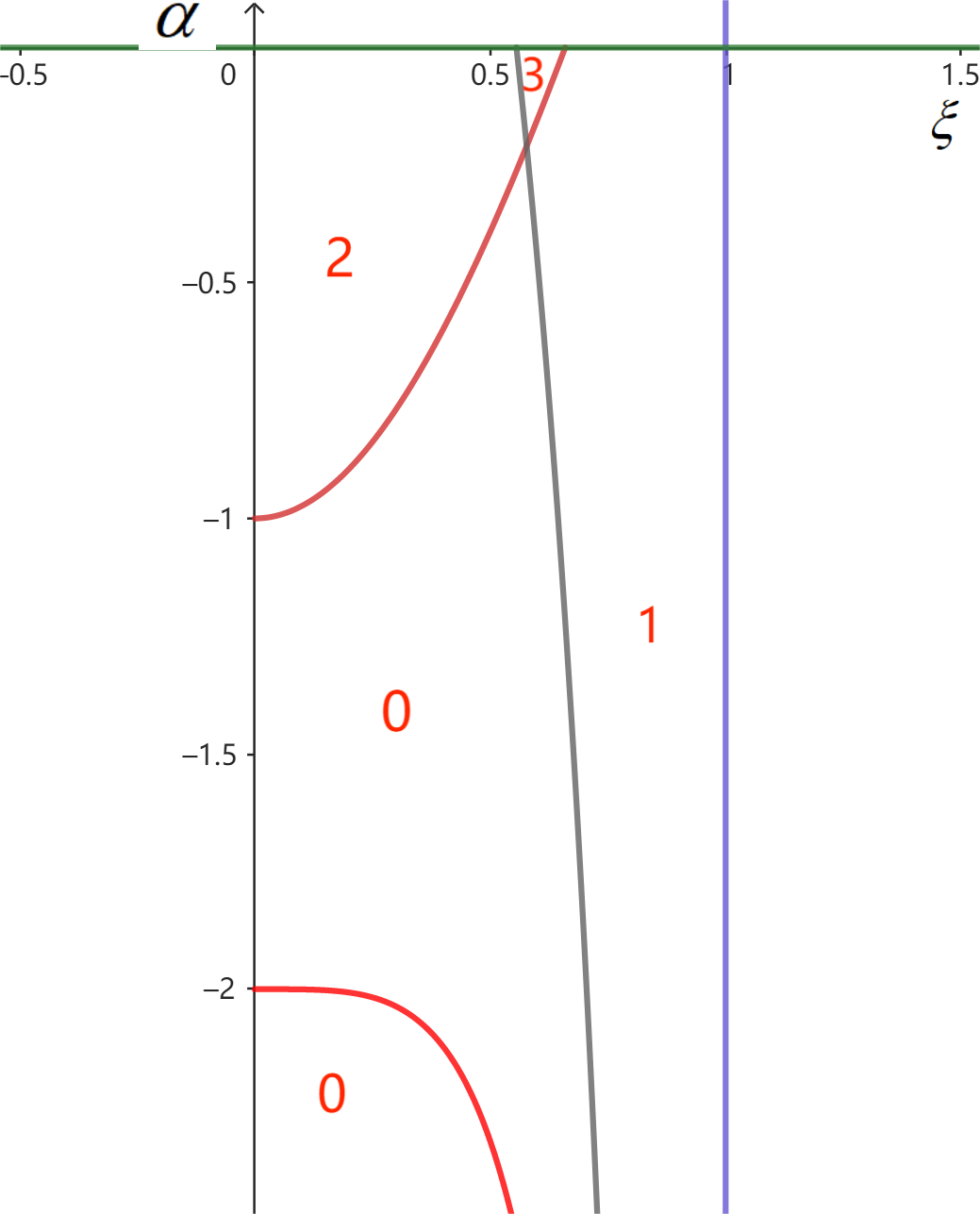
(b) (Sphere case $\alpha$ negative) In this figure are displayed the subregions of the $\widehat{\xi O\alpha}$-region $\Omega_{2}:=(1,+\infty)\times(-\infty,0)$ labeled by the Morse index of the corresponding circular orbit

Theorem 3.

(Hyperbolic plane Case) Let $p$ and $q$ be as in (1.3). For any $n\in\mathbb{N}$ there exists a circular solution $x_{n}$ with Morse index equal to $2n$. In the following figure are displayed the first index jump regions.

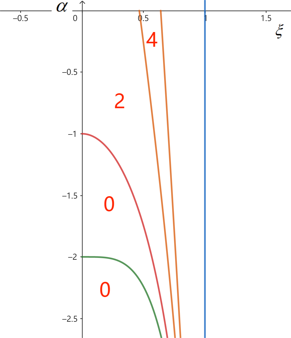
Figure 2: (Hyperbolic plane case) In the figure we represent the subregions of the $\Omega_{3}$ corresponding to the jumps of the Morse index.

We remark that in the Euclidean case we recover the results about the computation of the Morse index as well as an instability result for these class of solutions, already proved in [BJP16] and [KOP21].

Theorem 4.

Let $p(\xi)=1$, $q(\xi)=\xi^{\alpha}$ and let $x$ be a circular solution. Then, the Morse index of $x$ is given by

$$m^{-}(x)=\begin{cases}0&\textrm{ if }\quad\alpha\in(-\infty,-1]\\ 2&\textrm{ if}\quad\alpha\in(-1,0)\end{cases}.$$ (1.6)

Remark 1.1.

The case $\alpha=-1$ corresponds to the classical singular gravitational potential. In this case, we have

$$\iota_{1}(\gamma)=0$$ (1.7)

and the corresponding circular orbit is linearly unstable.

2 Surfaces of revolutions, radial functions and geodesics

Central potentials are extremely important in physics. It is well known that a particle moving in the Euclidean space and subject to a central force is confined to move in the plane spanned by its initial position and velocity. From the mathematical point of view, this means that the system is completely integrable and the angular momentum is a conserved quantity. It is thus natural to look for systems (and geometries) in which these symmetries are still present. A big class of $2D$ examples is given by revolution surfaces. They posses a natural $\mathbb{S}^{1}$ symmetry and a corresponding $\mathbb{S}^{1}$ action by isometry. We will consider potentials invariant with respect to it, i.e. depending solely on the distance from the fixed points of this action.

2.1 Radially conformal flat metrics on the plane

In the Euclidean three dimensional space $(\mathbb{E}^{3},g_{e})$ equipped with a Cartesian reference frame, we denote a point $P$ by the vector $(x_{0},x_{1},x_{2})\in\mathbb{R}^{3}$. We let $\ell_{i}$ to be the straight line corresponding to the $i$-th coordinate and we denote by $\Pi_{i,j}$ the plane spanned by $\ell_{i}$ and $\ell_{j}$ for $i,j=0,1,2$.

Given a smooth curve $\gamma:[-1,1]\to\mathbb{R}^{3}$, we assume

1. $\gamma$ is simple, namely $\gamma(t)=\gamma(s)$ iff $t=s$ and regular meaning that $\dot{\gamma}(t)\neq 0$, for every $t\in[-1,1]$

2. $\gamma([-1,1])$ is contained in the $\Pi_{0,2}$-plane whose ends are two distinct points on the $\ell_{2}$-axis

3. $\dot{\gamma}_{+}(-1),\ \dot{\gamma}_{-}(1)$ belongs to $\Pi_{0,1}$-plane where $\dot{\gamma}_{+}$ (resp. $\dot{\gamma}_{-}$) denotes the right (resp. left) derivative

Because of (C2), in local coordinates $\gamma$ is pointwise defined by $\gamma(t)=\big{(}x_{0}(t),0,x_{2}(t)\big{)}$ for $t\in[-1,1]$. We set

$$\Gamma:=\Set{\gamma\in\mathscr{C}^{\infty}([-1,1],\mathbb{E}^{3})}{(C1)-(C4)\textrm{ hold}}\quad\textrm{ and }\Sigma:=\Set{M_{\gamma}:=G\cdot\gamma}{\gamma\in\Gamma}\\ \textrm{ where }$G$\textrm{ denotes the group of isometries of $\mathbb{E}^{3}$ fixing the line $\ell_{2}$}.$$ (2.1)

By the properties of $\gamma$, it follows that $M_{\gamma}$ is diffeomorphic to the $2$-dimensional sphere $\mathbb{S}^{2}$ and because of (C3), we get that $M_{\gamma}$ is a smooth surface. We refer to the curve $\gamma$ as the generating curve of $M_{\gamma}$ and the circles described by the points of $\gamma$ correspond to the parallels of $M_{\gamma}$. We denote by $\widehat{M}_{\gamma}:=M_{\gamma}\setminus(\ell_{2}\cap M_{\gamma})$. Denoting by $A$ the degenerate skew-symmetric matrix corresponding to the infinitesimal generator of the group $G$, given by $A=\begin{bmatrix}0&-1&0\\ 1&0&0\\ 0&0&0\end{bmatrix}$, we get a surjective diffeomorphism between the open cylinder $\mathbb{S}^{1}\times(-1,1)$ and $\widehat{M}_{\gamma}$ defined by

$$\phi:\mathbb{S}^{1}\times(-1,1)\ni(t,\exp{(A\,\theta)})\longmapsto\exp{(A\,\theta)}\,\gamma(t)\in\widehat{M}_{\gamma}.$$

By means of this diffeomorphism we define a Riemannian metric $\widehat{g}_{\gamma}$ on $\widehat{M}_{\gamma}$ by pulling back the Euclidean Riemannian metric on $\mathbb{E}^{3}$ to $\widehat{M}_{\gamma}$. By an explicit calculations, we get that

$$g_{e}(\exp{(A\,\theta)}\dot{\gamma},\exp{(A\,\theta)}\dot{\gamma})=|\dot{\gamma}|^{2},\qquad g_{e}(A\exp{(A\,\theta)}\gamma,A\exp{(A\,\theta)}\gamma)=g_{e}(A\gamma,A\gamma)=x_{0}(t)^{2}\\ g_{e}(\exp{(A\,\theta)}\dot{\gamma},A\exp{(A\,\theta)}\gamma)=g_{e}(\dot{\gamma},A\gamma)=0.$$ (2.2)

As consequence of this discussion, we get that the Riemannian metric $\widehat{g}_{\gamma}$ on $\widehat{M}_{\gamma}$ in these new cylindrical coordinates, is given by

$$\widehat{g}_{\gamma}=\phi^{*}g_{e}=x_{0}(t)^{2}d\theta^{2}+|\dot{\gamma}|^{2}dt^{2}$$

where, as usually $\phi^{*}$ denotes the pull-back.

Proposition 2.1.

There exists a radial function $r\mapsto a(r)$ on $\mathbb{R}^{2}\setminus\{(0,0)\}$ such that $(\widehat{M}_{\gamma},\widehat{g}_{\gamma})$ is isometric to $(\mathbb{R}^{2},a^{2}(r)g_{e})$.

Proof.

We start by observing that, repeating verbatim the previous discussion once replaced $M_{\gamma}$ by $\mathbb{S}^{2}$, we can construct the diffeomorphism from the open cylinder $\mathbb{S}^{1}\times(-1,1)$ to $\widehat{\mathbb{S}^{2}}:=\mathbb{S}^{2}\setminus\{N,S\}$ where $N,S$ denote the north and the south poles respectively. Namely

$$\phi:\mathbb{S}^{1}\times(-1,1)\ni(t,\exp{(A\,\theta)})\longmapsto\exp{(A\,\theta)}\,\widetilde{\gamma}(t)\in\mathbb{S}^{2},$$

where $\widetilde{\gamma}$ is the curve defined by

$$\widetilde{\gamma}:[-1,1]\to\mathbb{R}^{3},\quad\tilde{\gamma}(t)=\left(\sqrt{1-t^{2}},0,t\right).$$ (2.3)

Denote by $\widehat{\mathbb{R}^{2}}:=\mathbb{R}^{2}\setminus\{(0,0)\}$ and let $\psi$ be the inverse of the stereographic projection from the north pole of $\mathbb{S}^{2}$. It is given explicitly by:

$$\psi:\widehat{\mathbb{R}^{2}}\ni(u,v)\longmapsto\left(\dfrac{2u}{1+u^{2}+v^{2}},\dfrac{2v}{1+u^{2}+v^{2}},\dfrac{u^{2}+v^{2}-1}{1+u^{2}+v^{2}}\right)\in\widehat{\mathbb{S}^{2}}.$$

The map $\widetilde{\phi}^{-1}\circ\psi:\mathbb{R}^{2}\to(-1,1)\times\mathbb{S}^{1}$ with respect to the local system of coordinates $(u,v)$ is given by

$$\widetilde{\phi}^{-1}\circ\psi(u,v)=(t(u,v),\theta(u,v))=\left(\dfrac{u^{2}+v^{2}-1}{1+u^{2}+v^{2}},\arctan\left(\dfrac{u}{v}\right)\right).$$

If $\sigma:\widehat{\mathbb{R}^{2}}\to\widehat{\mathbb{R}^{2}}$ is the polar change of coordinates defined by

$$\sigma(\rho,\alpha)=\big{(}\sqrt{u^{2}+v^{2}},\arctan(u/v)\big{)}$$

and denoting by $F$ the diffeomorphism given by

$$F=\widetilde{\phi}^{-1}\circ\psi\circ\sigma:\widehat{\mathbb{R}^{2}}\ni(\rho,\alpha)\longmapsto(t(\rho,\alpha),\theta(\rho,\alpha))=\left(\dfrac{\rho^{2}-1}{1+\rho^{2}},\alpha\right)\in\mathbb{S}^{1}\times(-1,1)$$

since $g_{\gamma}=\phi^{*}g_{e}$, we finally get

$$F^{*}\widehat{g}_{\gamma}=\left(\dfrac{4\rho^{2}}{(1+\rho^{2})^{2}}\right)^{2}|\dot{\gamma}(t(\rho))|^{2}d\rho^{2}+x_{0}(t(\rho))^{2}d\alpha^{2}.$$

To conclude the proof of the first claim, we introduce a suitable time rescaling along the curve $\gamma$.

Let $\lambda$ be a reparametrization of the time variable $t$ and let us denote by ^′ the new time variable $s$. Thus we get that

$$\widehat{g}_{\gamma}=|\gamma^{\prime}(\lambda(s))|^{2}\lambda^{\prime}(s)^{2}ds^{2}+x_{0}(\lambda(s))^{2}d\theta^{2}\quad\textrm{ and}\\ F^{*}\widehat{g}_{\gamma}=\dfrac{x_{0}(\lambda(s))^{2}}{\rho^{2}}\left[\left[\dfrac{4\rho^{2}}{(1+\rho^{2})^{2}}\right]^{2}\dfrac{\lambda^{\prime 2}|\gamma^{\prime}(\lambda(s))|^{2}}{x_{0}(\lambda(s))^{2}}d\rho^{2}+\rho^{2}d\alpha^{2}\right].$$ (2.4)

Thus, imposing that $F^{*}g_{\gamma}$ is conformal to the flat metric, uniquely determines $\lambda$. For, we let

$$\lambda^{\prime}(s(\rho))=\left(\dfrac{1+\rho^{2}}{2\rho}\right)^{2}\dfrac{x_{0}(\lambda(s(\rho)))}{|\gamma^{\prime}(\lambda(s(\rho)))|}\quad\textrm{ where }\quad s(\rho)=\dfrac{\rho^{2}-1}{\rho^{2}+1}.$$

With such a choice it readily follows that

$$F^{*}\widehat{g}_{\gamma}=\dfrac{x(\lambda(s))^{2}}{\rho^{2}}\big{(}d\rho^{2}+\rho^{2}d\alpha^{2}\big{)}.$$

which concludes the proof. ∎

2.2 Meridians and geodesics

On a surface of revolution, there are two families of distinguished geodesics: parallels and meridians. The first ones are orbits of the $\mathbb{S}^{1}$ action whereas the second ones are all the geodesics issuing from fixed points. The next Proposition shows this and provides and integral expression for the Riemannian distance.

Proposition 2.2.

Let su consider $(\mathbb{R}^{2},g)$ where

$$g:=a^{2}(r)g_{e},\text{ and }\quad a(r)>0$$

and let $X$ be the radial vector field given by $X:=a(r)^{-1}\partial_{r}$. Then we have

$$\nabla_{X}X=0$$

and its integral curves are unit speed geodesics through the origin. Moreover, solutions starting from the origin are minimizing geodesics. The (Riemannian) distance of a point $x$ from origin is given by:

$$d_{a}(0,x)=\int_{0}^{|x|}{a(t)}dt$$ (2.5)

where $|\cdot|$ denotes the Euclidean norm.

Proof.

Since $|X|_{g}=1$, its integral curves are unit speed curves. To check the geodesic condition we have to compute $\nabla_{X}X$. Standard differential formulas involving conformal changes of the type $g=e^{2\log a}g_{e}$, of the metric yield:

$$\nabla_{X}X=\nabla^{e}_{X}X+2g_{e}(\nabla\log(a),X)X-g_{e}(X,X)\nabla\log(a)$$

where $\nabla^{e}$ denotes the Levi-Civita connection with respect to the Euclidean metric. A direct computation yields:

$$\nabla^{e}_{X}X=a^{-2}(r)\nabla_{\partial_{r}}\partial_{r}+a^{-1}(\partial_{r}a^{-1}(r))\partial_{r}=-(\partial_{r}a)a^{-3}\partial_{r}.$$

Since $\nabla\log(a)=a^{-1}\partial_{r}a$ and $g_{e}(X,X)=a^{-2}$. Summing up the above computations, we get $\nabla_{X}X=0$. By this we immediately get that $\gamma$ is a unit speed geodesic.

Now, we prove that the straightlines from the origin are minimizing. Let $\eta$ be any curve joining $0$ to a point $x$ then, in coordinates $\theta$ and $r$ we can write $\eta=r(t)e^{i\theta(t)}$. It follows that

$$|\dot{\eta}|_{g}=a(r)\sqrt{\dot{r}+r^{2}\dot{\theta}}\geq a(r)|\dot{r}|.$$

On the other hand, if $x=r_{0}e^{i\theta_{0}}$, the curve $\tilde{\eta}(t)=r(t)e^{i\theta_{0}}$ satisfies the same boundary conditions but $\ell(\eta)\geq\ell(\tilde{\eta})$. It follows that minimizing geodesic from $0$ to the point $x$ are straight lines.

Take an integral line $\eta$ of $X$ joining $0$ to a point $x$. Since $X$ gives arclength parametrized geodesics and since along a straight geodesic starting at the origin, we get that $|\eta|_{g}=a(r)\dot{r}=1$ we have by integrating over $[0,T]$:

$$a(r)\dot{r}=1\Rightarrow d(0,x)=T=\int_{0}^{T}a(r)\dot{r}dt\underset{[s=r(t)]}{=}\int_{0}^{r(T)}a(s)ds=\int_{0}^{|x|}a(s)ds.$$

∎

One direct consequence of Proposition 2.2, is that we can, in principle, rewrite any radial function defined in $\mathbb{R}^{2}$ as a function of the Riemannian distance by looking at $r$ as function of $d(0,x)$ through Equation (2.5). Although, in general, it is not possible to get a closed form for $r$ as a function of the Riemannian distance, in the cases we are interested in, corresponding to constant curvature surfaces, this is possible and will be the starting point of the next section.

2.3 Central force problem on constant curvature surfaces

We start by considering the configuration space $(\mathbb{R}^{2},g)$, equipped with polar coordinates $(r,\vartheta)$, where $g$ is a conformally flat metric and we denote by $\mathbb{S}^{2}_{R}$ (resp. $\mathbb{H}^{2}_{R}$) the sphere (resp. the pseudo-sphere) of radius $R$. The conformal factor is given by

$$\mu_{R}(r):=\begin{cases}\dfrac{2R^{2}}{R^{2}+r^{2}}&\textrm{ for $\mathbb{S}^{2}_{R}$ }\\[7.0pt] \dfrac{2R^{2}}{R^{2}-r^{2}}&\textrm{ for $\mathbb{H}^{2}_{R}$ }\\[5.0pt] \end{cases}$$

In terms of the curvature $\kappa$, the conformal factor can be written at once as

$$\mu_{R}(r)=\dfrac{2}{1+\kappa r^{2}}\quad\textrm{ where }\quad\kappa=\begin{cases}1/R^{2}&\textrm{ for the sphere}\\ -1/R^{2}&\textrm{ for the pseudosphere}\end{cases}$$

We now take the origin as the center of the central force and we consider the simple mechanical system $(M,g,V)$ where $M:=\mathbb{R}^{2}\setminus\{(0,0)\}$ and $V:M\to\mathbb{R}$ is a power law potential energy (independent on $\vartheta$) depending only on the Riemannian distance from the origin. By taking into account Proposition 2.2 and by a direct integration of the conformal factor, we get that the distance of the point $P(r,\vartheta)$ to the origin is

$$d_{R}(r)=\begin{cases}2R\arctan(r/R)&\textrm{ for }\quad\mathbb{S}^{2}_{R}\\[7.0pt] R\ln\left(\dfrac{R+r}{R-r}\right)&\textrm{ for }\quad\mathbb{H}^{2}_{R}\end{cases}$$

Given $\alpha\in\mathbb{R}^{*}$, we let

$$V_{\alpha}:M\to\mathbb{R}\quad\textrm{ defined by }\quad V_{\alpha}(r,\vartheta)=-m\,[d_{R}(r)]^{\alpha}\qquad m\in(0,+\infty)$$

and we consider the Lagrangian $\widetilde{L}_{\alpha}$ of the mechanical system $(M,g,V_{\alpha})$ on the state space $TM$ given by

$$\widetilde{L}_{\alpha}(r,\vartheta,v_{r},v_{\vartheta})=\dfrac{1}{2}\mu_{R}^{2}(r)(v_{r}^{2}+r^{2}v_{\vartheta}^{2})-V_{\alpha}(r,\vartheta)$$

By setting $\xi:=r/R$, then the Lagrangian function can be written, as follows

$$\widetilde{L}_{\alpha}(\xi,\vartheta,v_{\xi},v_{\vartheta}):=\begin{cases}\dfrac{2R^{2}}{(1+\xi^{2})^{2}}\Big{[}v_{\xi}^{2}+\xi^{2}v_{\vartheta}^{2}\Big{]}+m\big{[}2R\arctan\xi]^{\alpha}&\textrm{ for }\mathbb{S}^{2}_{R}\\[12.0pt] \dfrac{2R^{2}}{(1-\xi^{2})^{2}}\Big{[}v_{\xi}^{2}+\xi^{2}v_{\vartheta}^{2}\Big{]}+m\left[R\ln\left(\dfrac{1+\xi}{1-\xi}\right)\right]^{\alpha}&\textrm{ for }\mathbb{H}^{2}_{R}.\end{cases}$$

Now, computing $\widetilde{L}_{\alpha}$ along a smooth curve and rescaling time by setting

$$t:=\begin{cases}\big{(}m\,2^{\alpha{-1}}\,R^{\alpha-2}\big{)}^{-1/2}\tau&\textrm{ in the case of }\mathbb{S}^{2}_{R}\\[12.0pt] \left(m\,{2^{-1}}\,R^{\alpha-2}\right)^{-1/2}\tau&\textrm{ in the case of }\mathbb{H}^{2}_{R}\end{cases}$$

by abusing notation and denoting by $\cdot$ the $\tau$ derivative as well, we get that $\widetilde{L}_{\alpha}=C_{\alpha}\,L_{\alpha}$ where

$$L_{\alpha}(\xi,\vartheta,\dot{\xi},\dot{\vartheta}):=\begin{cases}\dfrac{1}{(1+\xi^{2})^{2}}\Big{[}\dot{\xi}^{2}+\xi^{2}\dot{\vartheta}^{2}\Big{]}+\arctan^{\alpha}\xi&\textrm{ in the case of }\mathbb{S}^{2}_{R}\\[12.0pt] \dfrac{1}{(1-\xi^{2})^{2}}\Big{[}\dot{\xi}^{2}+\xi^{2}\dot{\vartheta}^{2}\Big{]}+\ln^{\alpha}\left(\dfrac{1+\xi}{1-\xi}\right)&\textrm{ in the case of }\mathbb{H}^{2}_{R}\end{cases}$$

and $C_{\alpha}:=mR^{\alpha}2^{\alpha}$ (resp. $C:=mR^{\alpha}$) in the case of $\mathbb{S}_{R}^{2}$ (resp. $\mathbb{H}_{R}^{2}$).

2.4 Euler-Lagrange equation and Sturm-Liouville problem

We let $p_{\pm}(\xi):=2(1\pm\xi^{2})^{-2}$, $q_{+}(\xi):=\arctan^{\alpha}\xi$ and $q_{-}(\xi):=\ln^{\alpha}\left(\frac{1+\xi}{1-\xi}\right)$.

Notation 2.3.

In shorthand notation, with abuse of notation, we use $p(\xi)$ for denoting either $p_{+}(\xi)$ or $p_{-}(\xi)$ and $q(\xi)$ for denoting either $q_{+}(\xi)$ or $q_{-}(\xi)$. Furthermore, we denote by $p^{\prime}$ (resp. $q^{\prime}$) the $\xi$ derivative of $p$ (resp. $q$).

Bearing this notation in mind and once observed that without loss of generality we can consider the Lagrangian $L_{\alpha}$ instead of $\widetilde{L}_{\alpha}$, given by

$$L_{\alpha}(\xi,\vartheta,\dot{\xi},\dot{\vartheta})=\dfrac{1}{2}p(\xi)\big{[}\dot{\xi}^{2}+\xi^{2}\dot{\vartheta}^{2}\big{]}+q(\xi).$$ (2.6)

and by a direct calculation we get that the associated Euler-Lagrangian equation is

$$\begin{cases}\dfrac{d}{d\tau}(p\,\dot{\xi})=\dfrac{1}{2}p^{\prime}(\dot{\xi}^{2}+\xi^{2}\dot{\vartheta}^{2})+p\,\xi\dot{\vartheta}^{2}+\,q^{\prime}\qquad\textrm{ on }[0,T]\\[10.0pt] \dfrac{d}{d\tau}(p\,\xi^{2}\dot{\vartheta})=0.\end{cases}$$ (2.7)

A special class of solutions of the Euler-Lagrange equation, is provided by the circular solutions pointwise defined by $\gamma_{0}(t)=\big{(}\xi_{0},\vartheta(t)\big{)}$, where by the first equation of (2.7), we immediately get

$$\dot{\vartheta}^{2}=\dfrac{-2q^{\prime}}{(p\,\xi^{2})^{\prime}}\Big{|}_{\xi=\xi_{0}}.$$ (2.8)

Notation 2.4.

We set

$$p_{0}\coloneqq p(\xi_{0}), p^{\prime}_{0}\coloneqq p^{\prime}(\xi_{0}), p^{\prime\prime}_{0}\coloneqq p^{\prime\prime}(\xi_{0})$$ (2.9)

$$q_{0}\coloneqq q(\xi_{0}), q^{\prime}_{0}\coloneqq q^{\prime}(\xi_{0}), q^{\prime\prime}_{0}\coloneqq q^{\prime\prime}(\xi_{0})$$ (2.10)

$$\eta_{0}\coloneqq p_{0}\,\xi_{0}^{2} \eta_{0}^{\prime}\coloneqq(p_{0}\,\xi_{0}^{2})^{\prime}=p^{\prime}_{0}\xi_{0}^{2}+2p_{0}\,\xi_{0} \dot{\vartheta}_{0}^{2}=-2q_{0}^{\prime}\,{\eta^{\prime}}_{0}^{-1}.$$ (2.11)

So, the period $T$ is given by

$$T=2\pi\,\omega_{0}\quad\textrm{ where }\quad\omega_{0}:=\left.\sqrt{\dfrac{\eta^{\prime}}{-2q^{\prime}}}\right|_{\xi=\xi_{0}}$$ (2.12)

By linearizing along $\gamma_{0}$ we get the Sturm-Liouville equation given by

$$-\dfrac{d}{d\tau}\big{(}P\dot{y}+Qy\big{)}+{Q}^{\mathsf{T}}\dot{y}+Ry=0\quad\textrm{ on }\quad[0,T]$$

where

$$P=\begin{bmatrix}p_{0}&0\\ 0&\eta_{0}\end{bmatrix},\qquad Q=\begin{bmatrix}0&0\\ \zeta_{0}&0\end{bmatrix}\quad\textrm{ where }\quad\zeta_{0}:=\begin{cases}\sqrt{-2q_{0}^{\prime}\,\eta_{0}^{\prime}},&\quad\textrm{ if }\quad\eta^{\prime}_{0}\geq 0\\[7.0pt] -\sqrt{-2q_{0}^{\prime}\,\eta_{0}^{\prime}},&\quad\textrm{ if }\quad\eta^{\prime}_{0}<0\end{cases}\textrm{ and finally}\\[7.0pt] R=\begin{bmatrix}R_{11}&0\\ 0&0\end{bmatrix}\quad\textrm{ for }\quad R_{11}:=\eta_{0}^{\prime}\cdot\left[\dfrac{q_{0}^{\prime}}{\eta_{0}^{\prime}}\right]^{\prime}$$ (2.13)

We set $B=\begin{bmatrix}P^{-1}&-P^{-1}Q\\ -{Q}^{\mathsf{T}}P^{-1}&{Q}^{\mathsf{T}}P^{-1}Q-R\end{bmatrix}$. By a direct computation, we get

$$P^{-1}=\begin{bmatrix}p^{-1}_{0}&0\\ 0&\eta_{0}^{-1}\end{bmatrix}\qquad P^{-1}Q=\begin{bmatrix}0&0\\ \eta_{0}^{-1}\cdot\zeta_{0}&0\end{bmatrix}\\[10.0pt] {Q}^{\mathsf{T}}P^{-1}Q=\begin{bmatrix}\eta_{0}^{-1}\cdot\zeta_{0}^{2}&0\\ 0&0\end{bmatrix}\qquad{Q}^{\mathsf{T}}P^{-1}Q-R=\begin{bmatrix}\eta_{0}^{-1}\cdot\zeta_{0}^{2}-\eta_{0}^{\prime}\cdot(q_{0}^{\prime}/\eta_{0}^{\prime})^{\prime}&0\\ 0&0\end{bmatrix}.$$ (2.14)

We observe that

$$\eta_{0}^{-1}\,\zeta_{0}^{2}=-2\,q_{0}^{\prime}\,\big{(}\ln\eta_{0}\big{)}^{\prime}\qquad\eta_{0}^{-1}\,\zeta_{0}=\sqrt{2\,q_{0}^{\prime}(\eta_{0}^{-1})^{\prime}}\qquad\textrm{ and }\\ \eta_{0}^{-1}\,\zeta_{0}^{2}-R_{11}=-2q_{0}^{\prime}\,(\ln\eta_{0})^{\prime}-\eta_{0}^{\prime}\left(\dfrac{q_{0}^{\prime}}{\eta_{0}^{\prime}}\right)^{\prime}$$ (2.15)

In conclusion, we get

$$B=\begin{bmatrix}p_{0}^{-1}&0&0&0\\ 0&\eta_{0}^{-1}&-\eta_{0}^{-1}\cdot\zeta_{0}&0\\ 0&-\eta_{0}^{-1}\cdot\zeta_{0}&-2q_{0}^{\prime}\,(\ln\eta_{0})^{\prime}-\eta_{0}^{\prime}\left(\dfrac{q_{0}^{\prime}}{\eta_{0}^{\prime}}\right)^{\prime}&0\\ 0&0&0&0\end{bmatrix}\textrm{ and }\\ JB=\begin{bmatrix}0&\eta_{0}^{-1}\cdot\zeta_{0}&2q_{0}^{\prime}\,(\ln\eta_{0})^{\prime}+\eta_{0}^{\prime}\left(\dfrac{q_{0}^{\prime}}{\eta_{0}^{\prime}}\right)^{\prime}&0\\ 0&0&0&0\\ p_{0}^{-1}&0&0&0\\ 0&\eta_{0}^{-1}&-\eta_{0}^{-1}\cdot\zeta_{0}&0\end{bmatrix}$$ (2.16)

where $J:=\begin{bmatrix}0&-I_{2}\\ I_{2}&0\end{bmatrix}$ denotes the standard complex structure.

3 The generalized Conley-Zehnder index and normal forms

This section is devoted to provide a complete proof of the following result.

Theorem 3.1.

Let $a,b,c,d\in\mathbb{R}$, $a$ positive, we let

$$A=\begin{bmatrix}0&b&d&0\\ 0&0&0&0\\ a&0&0&0\\ 0&c&-b&0\end{bmatrix}$$

and we denote by $\gamma$ the fundamental solution of the following linear Hamiltonian system

$$\dot{z}(t)=Az(t)\qquad t\in[0,T].$$ (3.1)

Then the generalized Conley-Zehnder index $\iota_{1}(\gamma(t),t\in[0,T])$ is given by

$$\iota_{1}(\gamma(t),t\in[0,T])=\begin{cases}2k&\textrm{ if }\quad d<0\textrm{ and }cd+b^{2}\geq 0\\[10.0pt] 2k+1&\textrm{ if }\quad d<0\textrm{ and }cd+b^{2}<0\\[10.0pt] 0&\textrm{ if }\quad\begin{cases}d=0,\ b=0\textrm{ and }c>0\\ d=0\textrm{ and }b\neq 0\\ d>0\textrm{ and }cd+b^{2}>0\end{cases}\\[20.0pt] -1&\textrm{if }\quad\begin{cases}d=0,\ b=0\textrm{ and }c\leq 0\\ d>0\textrm{ and }cd+b^{2}\leq 0\end{cases}\end{cases}$$ (3.2)

where $k\in\mathbb{N}$ is given by $k\cdot 2\pi<\sqrt{-ad}\cdot T\leq(k+1)\cdot 2\pi$.

Remark 3.2.

We observe that in the cases we are interested in $c>0$. A direct consequence of this fact, as expected, is that $\iota_{1}(\gamma)\geq 0$. In fact, the last case can be easily excluded by observing that, since $c>0$ and assuming $d>0$ as required in the last case, the term $cd+b^{2}>0$.

Proof of Theorem 3.1, will be done through an explicit computation of the normal forms and of the generalized Conley-Zehnder index for autonomous linear Hamiltonian vector field of the form $JB$. We refer to the Appendix A and references therein, for the basic definitions and properties of the generalized Conley-Zehnder index $\iota_{1}$, as well as the generalized Maslov index $\mu^{\scriptscriptstyle{\mathrm{CLM}}}$.

Notation 3.3.

We let

$$a\coloneqq p_{0}^{-1},\quad b\coloneqq\eta_{0}^{-1}\cdot\zeta_{0},\quad c\coloneqq\eta_{0}^{-1},\quad d\coloneqq 2q_{0}^{\prime}\,(\ln\eta_{0})^{\prime}+\eta_{0}^{\prime}\left(\dfrac{q_{0}^{\prime}}{\eta_{0}^{\prime}}\right)^{\prime}.$$ (3.3)

Bearing this notation in mind the linear autonomous Hamiltonian system $z^{\prime}(t)=JBz(t)$ reads as

$$\dot{z}(t)=Az(t)\qquad t\in[0,T]$$ (3.4)

where

$$A=\begin{bmatrix}0&b&d&0\\ 0&0&0&0\\ a&0&0&0\\ 0&c&-b&0\end{bmatrix}.$$ (3.5)

By a direct computation of the Cayley-Hamilton polynomial, we get that

$$\det(A-\lambda I)=\lambda^{2}(\lambda^{2}-ad)=0\quad\Rightarrow\lambda=0\quad\textrm{ or }\quad\lambda^{2}=ad$$

So, we have to split our discussion according to the sign of $d$.

First case: $d$ negative

Since, we have $ad<0$, the eigenvalues of matrix $A$ are

$$\lambda_{1}=\lambda_{2}=0,\qquad\lambda_{3}=\sqrt{-ad}\ i,\qquad\lambda_{4}=-\sqrt{-ad}\ i.$$ (3.6)

Since $0$ could have a non-trivial Jordan blocks, we discuss these two cases accordingly.

• Non-trivial Jordan block. This corresponds to the case $b^{2}+cd\neq 0$ since if this holds, then the $0$ eigenvalue is not semisimple.

  In this case, by the discussions in [CLW94, pag. 118-122], there exists a symplectic matrix $S\in\mathrm{Sp}(4,\mathbb{R})$ such that

  $$A=S\Big{(}\begin{bmatrix}0&s_{0}\\ 0&0\end{bmatrix}\diamond\begin{bmatrix}0&-\sqrt{-ad}\\ \sqrt{-ad}&0\end{bmatrix}\Big{)}S^{-1},$$ (3.7)

  where $s_{0}$ is a constant that will be determined later. In this case the fundamental solution $\gamma$ of the system given in Equation (3.4) splits as follows

  $$\gamma(t)=S(\gamma_{1}(t)\diamond\gamma_{2}(t))S^{-1},$$ (3.8)

  where $\gamma_{1}(t)\coloneqq\begin{bmatrix}1&s_{0}t\\ 0&1\end{bmatrix}$ and $\gamma_{2}(t)\coloneqq R(\sqrt{-ad}t)$ denotes a rotation matrix. By Lemma A.5, in order to compute $\iota_{1}(\gamma)$ we only need to compute $\iota_{1}(\gamma_{1})$ and $\iota_{1}(\gamma_{2})$ respectively.

  By Lemma A.7, we have

  $$\iota_{1}(\gamma_{2})=1+2k\textrm{ where $k$ is such that }k\cdot 2\pi<\sqrt{-ad}\,T\leq(k+1)\cdot 2\pi.$$

  To compute the index $\iota_{1}(\gamma_{1})$, we only need to determine the sign of $s_{0}$. We start by observing that $e_{4}={(0,0,0,1)}^{\mathsf{T}}$ belongs to the kernel of $A$. Now, we assume that $v$ is the solution of $Av=e_{4}$ and that $\omega(e_{4},v)=1$. Then we get that,

  $$v={(0,-1,b/d,x_{4})}^{\mathsf{T}}\qquad\textrm{ for }x_{4}\in\mathbb{R}.$$

  We let $S^{-1}=[s_{m,n}]_{m,n=1}^{4}$ and $M$ be the phase flow map at time-$1$, namely

  $$M=\begin{bmatrix}0&0&s_{0}&0\\ 0&0&0&-\sqrt{-ad}\\ 0&0&0&0\\ 0&\sqrt{-ad}&0&0\end{bmatrix}.$$

  Since $Ae_{4}=0$ and $S$ is invertible, then $MS^{-1}e_{4}=0$. By direct computations we have $S^{-1}e_{4}={(\alpha,0,0,0)}^{\mathsf{T}}$ and $\alpha\neq 0$. Let $S^{-1}v={(w_{1},w_{2},w_{3},w_{4})}^{\mathsf{T}}$. Using the equation $Av=\xi e_{4}$, we get $S^{-1}v={(v_{1},0,\beta\alpha/s_{0},0)}^{\mathsf{T}}$ where $\beta:=-(b^{2}+cd)/d$. Since $1=\omega(e_{4},v)=\omega(S^{-1}e_{4},S^{-1}v),$ then we conclude that $s_{0}=\beta\alpha^{2}$ and consequently the sign of $s_{0}$ is the same as the sign of $\beta$.

  Recall that $d<0$, then the sign of $s_{0}$ is the same as $cd+b^{2}$. Thus

  $$\iota_{1}(\gamma_{1})=\begin{cases}-1\quad&\textrm{ if }\quad cd+b^{2}>0\\ 0\quad&\textrm{ if }\quad cd+b^{2}<0.\end{cases}$$ (3.9)

  Consequently, by the additivity property of the $\iota_{1}$ index w.r.t. the symplectic product, we have

  $$\iota_{1}(\gamma)=\iota_{1}(\gamma_{1})+\iota_{1}(\gamma_{2})=\begin{cases}2k,\quad&\text{if}\quad cd+b^{2}>0\\ 1+2k,\quad&\text{if}\quad cd+b^{2}<0\\ \end{cases}$$ (3.10)

  where $k$ is determined by

  $$k\cdot 2\pi<\sqrt{-ad}\cdot T\leq(k+1)\cdot 2\pi.$$ (3.11)

• Trivial Jordan blocks. This corresponds to the case $b^{2}+cd=0$, since if this holds, then eigenvalue $0$ is semisimple.

  In this case, by the discussions in [CLW94, pag. 118-122], there exists a symplectic matrix $S\in\mathrm{Sp}(4,\mathbb{R})$ such that

  $$A=S\Big{(}\begin{bmatrix}0&0\\ 0&0\end{bmatrix}\diamond\begin{bmatrix}0&-\sqrt{-ad}\\ \sqrt{-ad}&0\end{bmatrix}\Big{)}S^{-1}.$$ (3.12)

  Let $\gamma(t)$ be the fundamental solution of system (3.4), then we have

  $$\gamma(t)=S(\gamma_{1}(t)\diamond\gamma_{2}(t))S^{-1},$$ (3.13)

  where $\gamma_{1}(t)=I$ and $\gamma_{2}(t)=R(\sqrt{-ad}t)$.

  By Lemma A.7 we have

  $$\iota_{1}(\gamma_{1})=-1,\iota_{1}(\gamma_{2})=1+2k\textrm{ where $k$ is given by }k\cdot 2\pi<\sqrt{-ad}\,T\leq(k+1)\cdot 2\pi.$$

  Then by Lemma A.5 we have

  $$\iota_{1}(\gamma)=\iota_{1}(\gamma_{1})+\iota_{1}(\gamma_{2})=2k,$$ (3.14)

  where $k$ is obtained by $k\cdot 2\pi<\sqrt{-ad}\,T\leq(k+1)\cdot 2\pi$.

Second case: $d=0$

In this case the spectrum of $A$ is given by $0$ and $A$ is not semisimple. By direct computations we have

$$A^{2}=\begin{bmatrix}0&0&0&0\\ 0&0&0&0\\ 0&ab&0&0\\ -ab&0&0&0\end{bmatrix}\qquad A^{3}=\begin{bmatrix}0&0&0&0\\ 0&0&0&0\\ 0&0&0&0\\ 0&-ab^{2}&0&0\end{bmatrix}\textrm{ and }A^{j}=0\qquad\forall j\geq 4.$$ (3.15)

Then the fundamental solution of the system given at Equation (3.4) is given by

$$\gamma(t)=e^{At}=\begin{bmatrix}1&bt&0&0\\ 0&1&0&0\\ at&abt^{2}/2&1&0\\ -abt^{2}/2&ct-ab^{2}t^{3}/6&-bt&1\end{bmatrix}.$$ (3.16)

We let

$$M_{1,1}(t)=\begin{bmatrix}1&bt\\ 0&1\end{bmatrix}\qquad M_{2,1}(t)=\begin{bmatrix}at&abt^{2}/2\\ -abt^{2}/2&ct-ab^{2}t^{3}/6\end{bmatrix}\quad\textrm{ and }\quad M_{22}(t)=\begin{bmatrix}1&0\\ -bt&1\end{bmatrix}.$$

In this case we can rewrite $\gamma(t)$ as a two by two block matrix. The computation of the $\iota_{1}$ index can be done, for instance, by using Equation (A.6). Bearing in mind the notation given in Equation A.5 and formula given in Equation (A.6), we let $V=\mathrm{Gr}(I_{2})$. Then $V^{I}=\mathrm{Gr}(I_{2})$ and $W_{I}(V)=\mathrm{Gr}(I_{4})$. Since $M_{11}(0)=I_{2}$, then we have $S(0)=\mathbb{R}^{2}$. We need to compute $S(T)$ which is related to the coefficient $b$. For this reason, we have to split into two subcases.

• In this case $M_{11}(T)=I_{2}$ and consequently $S(T)=\mathbb{R}^{2}$. Being $M_{21}(0)=0$, then we have

  $${M}^{\mathsf{T}}_{11}M_{21}=0\qquad\Rightarrow\qquad m^{+}({M}^{\mathsf{T}}_{11}M_{21}|_{S(0)})=0$$ (3.17)

  Moreover, we have $M_{21}(T)=\begin{bmatrix}aT&0\\ 0&cT\end{bmatrix}$ and so

  $$m^{+}({M}^{\mathsf{T}}_{11}(T)M_{21}(T)|_{S(T)})=\begin{cases}1\quad&\textrm{ if }\quad c\leq 0\\ 2\quad&\textrm{ if }\quad c>0.\end{cases}$$ (3.18)

  So, by Formula (A.6), we get

  $$\mu^{\scriptscriptstyle{\mathrm{CLM}}}(\mathrm{Gr}(I_{4}),\mathrm{Gr}(\gamma(t))=\begin{cases}1-0+2-2=1,\quad&\textrm{ if}\quad c\leq 0\\ 2-0+2-2=2,\quad&\textrm{ if}\quad c>0\\ \end{cases}$$ (3.19)

  and by invoking Lemma A.6, then we conclude that

  $$\iota_{1}(\gamma(t))=\begin{cases}-1\quad&\textrm{ if }\quad c\leq 0\\ 0\quad&\textrm{ if }\quad c>0\end{cases}$$ (3.20)

• In this case $M_{11}(T)=\begin{bmatrix}1&bT\\ 0&1\end{bmatrix}$ and consequently $S(T)=\{{(x,0)}^{\mathsf{T}}\ |\ x\in\mathbb{R}\}$. Thus,

  $${M}^{\mathsf{T}}_{11}(T)M_{21}(T)=\begin{bmatrix}1&0\\ bT&1\end{bmatrix}\cdot\begin{bmatrix}aT&abT^{2}/2\\ -abT^{2}/2&cT-ab^{2}T^{3}/6\end{bmatrix}=\begin{bmatrix}aT&abT^{2}/2\\ \frac{ab}{2}T^{2}&cT+ab^{2}T^{3}/3\end{bmatrix}.$$ (3.21)

  Then, for every $X={(x,0)}^{\mathsf{T}}\in S(T)$ we have

  $$\left\langle{{M}^{\mathsf{T}}_{11}(T)M_{21}(T)X},{X}\right\rangle_{M}=\left\langle{\begin{bmatrix}aT&abT^{2}/2\\ abT^{2}/2&cT+ab^{2}T^{3}/3\end{bmatrix}\begin{bmatrix}x\\ 0\end{bmatrix}},{\begin{bmatrix}x\\ 0\end{bmatrix}}\right\rangle_{M}=aTx^{2}>0.$$ (3.22)

  Therefore, by (A.6) we have

  $$\mu^{\scriptscriptstyle{\mathrm{CLM}}}(Gr(I_{4}),Gr(\gamma(t))=1-0+2-1=2.$$ (3.23)

  By Lemma A.6 once again, we have

  $$\iota_{1}(\gamma)=\mu^{\scriptscriptstyle{\mathrm{CLM}}}(Gr(I_{4}),Gr(\gamma(t))-2=0.$$ (3.24)

Third case: $d$ positive

All eigenvalues of $A$ are $\lambda_{1}=\lambda_{2}=0$ and $\lambda_{3}=\sqrt{ad},\lambda_{4}=-\sqrt{ad}$. Since $0$ could have a non-trivial Jordan blocks, we discuss these two cases accordingly.

• Non-trivial Jordan block. If $b^{2}+cd\neq 0$, then eigenvalue $0$ is not semisimple.

  In this case, by the discussions in [CLW94, pag. 118-122], there exists a symplectic matrix $S\in\mathrm{Sp}(4,\mathbb{R})$ such that

  $$A=S\Big{(}\begin{bmatrix}0&s_{0}\\ 0&0\end{bmatrix}\diamond\begin{bmatrix}\sqrt{ad}&0\\ 0&-\sqrt{ad}\end{bmatrix}\Big{)}S^{-1},$$ (3.25)

  where $s_{0}$ is a constant that will be determined later. Let $\gamma(t)$ be the fundamental solution of system given at Equation (3.4). Then we have

  $$\gamma(t)=S(\gamma_{1}(t)\diamond\gamma_{2}(t))S^{-1},$$ (3.26)

  where $\gamma_{1}(t)=\begin{bmatrix}1&s_{0}t\\ 0&1\end{bmatrix}$ and $\gamma_{2}(t)=\begin{bmatrix}e^{\sqrt{ad}t}&0\\ 0&e^{-\sqrt{ad}t}\end{bmatrix}$. As before, by taking into account Lemma A.5, in order to compute $\iota_{1}(\gamma)$ we only need to compute $\iota_{1}(\gamma_{1})$ and $\iota_{1}(\gamma_{2})$ respectively.

  We start observing that for the path $t\mapsto\gamma_{2}(t)$ the unique crossing occurs at $t=0$ and, at this crossing, $\ker(\gamma(0)-I_{2})=\mathbb{R}^{2}$. Moreover, the crossing form is represented w.r.t. to the scalar product of $\mathbb{R}^{2}$ by the matrix $-J\dot{\gamma}(0)\gamma(0)^{-1}=\begin{bmatrix}0&-\sqrt{ad}\\ -\sqrt{ad}&0\end{bmatrix}$. By a straightforward computation we get that the eigenvalues $\pm\sqrt{ad}$ and since the contribution to the Maslov index at the starting point is provided by the co-index according to formula given at Equation (A.4), then we get that $\mu^{\scriptscriptstyle{\mathrm{CLM}}}(\Delta,\mathrm{Gr}\gamma_{2}(t),t\in[0,T])=1$. Consequently, by invoking Lemma (A.6), we finally get $\iota_{1}(\gamma_{2})=0$.

  For computing the index $\iota_{1}(\gamma_{1})$, we only need to determine the sign of $s_{0}$. Since the discussion is precisely the same as before will be left to the reader. We just mention that, in this case, the sign of $s_{0}$ coincides with that of $-(cd+b^{2})$. Thus, we get

  $$\iota_{1}(\gamma_{1})=\begin{cases}0,\quad&\text{if}\quad cd+b^{2}>0\\ -1,\quad&\text{if}\quad cd+b^{2}<0\end{cases}$$ (3.27)

  Consequently, we have

  $$\iota_{1}(\gamma)=\iota_{1}(\gamma_{1})+\iota_{1}(\gamma_{2})=\begin{cases}0,\quad&\text{if}\quad cd+b^{2}>0\\ -1,\quad&\text{if}\quad cd+b^{2}<0\end{cases}$$ (3.28)

• Trivial Jordan block. If $b^{2}+cd=0$, then the $0$ eigenvalue is semisimple.

  In this case, by the normal form classification given at [CLW94, page 118-122], there exists a symplectic matrix $S\in\mathrm{Sp}(4,\mathbb{R})$ such that

  $$A=S\Big{(}\begin{bmatrix}0&0\\ 0&0\end{bmatrix}\diamond\begin{bmatrix}\sqrt{ad}&0\\ 0&-\sqrt{ad}\end{bmatrix}\Big{)}S^{-1}.$$ (3.29)

  By the very same computation as before, we get $\iota_{1}(\gamma_{1})=-1$ and $\iota_{1}(\gamma_{2})=0$. Then by using once again Lemma A.5, then we get

  $$\iota_{1}(\gamma)=\iota_{1}(\gamma_{1})+\iota_{1}(\gamma_{2})=-1.$$ (3.30)

Proof of Theorem 3.1

The proof of this result readily follows by summing up Equation (3.10), Equation (3.14), Equation (3.20), Equation (3.24), Equation (3.28) and finally Equation (3.30), concluding the proof.

Proof of Theorem 1

The proof of this result is direct consequence of Theorem 3.1 and Theorem A.8.

4 Computations of Maslov index for circular orbits

This section is devoted to compute the generalized Conley-Zehnder index of the circular orbits on the sphere, pseudo-sphere and Euclidean plane. This will be achieved by using Theorem 3.1 and the computation provides in Section 3. So, the main issues is to explicitly compute the constants $a,b,c,d$ appearing in the aforementioned theorem.

We start by recalling that, in this case, the Lagrangian of the problem is given by

$$L(\xi,\vartheta,\dot{\xi},\dot{\vartheta})=\dfrac{1}{2}p(\xi)\big{[}\dot{\xi}^{2}+\xi^{2}\dot{\vartheta}^{2}\big{]}+q(\xi).$$ (4.1)

4.1 Circular orbits on the sphere

In this case $p(\xi)=\dfrac{2}{(1+\xi^{2})^{2}}\textrm{ and }q(\xi)=\arctan^{\alpha}\xi$. In shorthand notation, we set $F(\xi):=\arctan\xi$. Bearing in mind the notation given in Equation (2.9), we get

$$p_{0}=2(1+\xi_{0}^{2})^{-2} p^{\prime}_{0}=-8\xi_{0}(1+\xi_{0}^{2})^{-3} p^{\prime\prime}_{0}=8(5\xi^{2}_{0}-1)(1+\xi_{0}^{2})^{-4}$$ (4.2)

$$q_{0}=F^{\alpha}(\xi_{0}) q^{\prime}_{0}=\alpha\cdot F^{\alpha-1}(\xi_{0})(1+\xi^{2}_{0})^{-1} q^{\prime\prime}_{0}=\dfrac{\alpha(\alpha-1)F^{\alpha-2}(\xi_{0})-2\alpha\xi_{0}F^{\alpha-1}(\xi_{0})}{(1+\xi^{2}_{0})^{2}}$$

$$\eta_{0}=2\xi_{0}^{2}(1+\xi_{0}^{2})^{-2} \eta_{0}^{\prime}=4\xi_{0}(1-\xi_{0}^{2})(1+\xi_{0}^{2})^{-3} \dot{\vartheta}_{0}^{2}=\dfrac{-\alpha F^{\alpha-1}(\xi_{0})(1+\xi_{0}^{2})^{2}}{2\xi_{0}(1-\xi_{0}^{2})}$$

In order for the (RHS) of $\dot{\vartheta}_{0}^{2}$ to be positive, we have to impose the following restriction on $\xi_{0}$:

$$\xi_{0}\in\begin{cases}(0,1)\quad&\text{if}\ \alpha<0,\\ (1,+\infty)\quad&\text{if}\ \alpha>0.\end{cases}$$ (4.3)

By a direct computation, we get

$$a=\dfrac{(1+\xi_{0}^{2})^{2}}{2} b=\dfrac{-2\xi_{0}^{2}+2}{\xi_{0}}\cdot\sqrt{\dfrac{-\alpha F^{\alpha-1}(\xi_{0})}{2\xi_{0}(1-\xi_{0}^{2})}}$$ (4.4)

$$c=\dfrac{(1+\xi_{0}^{2})^{2}}{2\xi_{0}^{2}} d=\dfrac{\alpha F^{\alpha-2}(\xi_{0})\{(3\xi_{0}^{4}-2\xi_{0}^{2}+3)\cdot F(\xi_{0})+(\alpha-1)\xi_{0}(1-\xi_{0}^{2})\}}{\xi_{0}(1+\xi_{0}^{2})^{2}(1-\xi_{0}^{2})}.$$

In order to determine the generalized Conley-Zehnder index, we have to discuss the sign of $d$ according to $\alpha$ and $\xi_{0}$.

First case: $\alpha$ positive

Since in this case $\xi_{0}\in(1,+\infty)$, then we get that the sign of $d$ is minus the sign of

$$f_{1}(\xi)=(3\xi^{4}-2\xi^{2}+3)\cdot\arctan\xi+(\alpha-1)\xi(1-\xi^{2}).$$ (4.5)

We let

$$\Omega_{1}\coloneqq(1,+\infty)\times(0,+\infty)$$ (4.6)

and we define the subregions

$$\Omega_{1}^{\pm}\coloneqq\Set{(\xi,\alpha)\in\Omega}{\pm f_{1}(\xi)>0}$$ (4.7)

whose separatrix is given by

$$\Omega_{1}^{0}=\Set{(\xi,\alpha)\in\Omega_{1}}{\alpha=1+\dfrac{(3\xi^{4}-2\xi^{2}+3)\arctan\xi}{\xi(\xi^{2}-1)}}.$$ (4.8)

We observe that the function $h$, defined by

$$h(\xi):=1+\dfrac{(3\xi^{4}-2\xi^{2}+3)\arctan\xi}{\xi(\xi^{2}-1)}$$

is convex, bounded below by constant $\alpha^{*}>1$ and such that

$$\lim_{\xi\to 1^{-}}h(\xi)=+\infty\qquad\textrm{ and }\qquad\lim_{\xi\to+\infty}h(\xi)=+\infty.$$

Moreover $h$ has an oblique asymptote defined by the equation

$$\alpha=\xi+1$$

Case: $(\xi_{0},\alpha)\in\Omega_{1}^{-}$.

Then we have $f_{1}(\xi_{0})<0$ and consequently by Equation (4.4), we get that $d>0$. Since $c$ is always strictly positive, then we have $b^{2}+cd>0$. By taking into account Equation (3.28), we have

$$\iota_{1}(\gamma)=0\qquad\text{if}\quad(\xi,\alpha)\in\Omega_{1}^{-}.$$ (4.9)

Case: $(\xi_{0},\alpha)\in\Omega_{1}^{0}$.

Then we have $f_{1}(\xi_{0})=0$ and consequently by using Equation (4.4) we have $d=0$. Since $c>0$, then by Equation (3.20) and Equation (3.24), we also have

$$\iota_{1}(\gamma)=0\qquad\text{if}\quad(\xi,\alpha)\in\Omega_{1}^{0}.$$ (4.10)

Case: $(\xi_{0},\alpha)\in\Omega_{1}^{+}$.

Then we have $f_{1}(\xi_{0})>0$ and consequently by Equation (4.4) we have $d<0$. Next we need to determine the sign of $b^{2}+cd$. Taking into account Equation (4.4) and after some algebraic manipulations, we have

$$b^{2}+cd =\dfrac{-\alpha F^{\alpha-2}(\xi_{0})\{(\xi_{0}^{4}-6\xi_{0}^{2}+1)\cdot F(\xi_{0})-(\alpha-1)\xi_{0}(1-\xi_{0}^{2})\}}{2\xi_{0}^{3}(1-\xi_{0}^{2})}.$$ (4.11)

We observe that, since $F(\xi_{0})$ is strictly positive and $1-\xi_{0}^{2}<0$, then the sign of $b^{2}+cd$ coincides with that of $(\xi_{0}^{4}-6\xi_{0}^{2}+1)\cdot F(\xi_{0})-(\alpha-1)\xi_{0}(1-\xi_{0}^{2})$. Let

$$f_{2}(\xi)=(\xi^{4}-6\xi^{2}+1)\arctan\xi-(\alpha-1)\xi(1-\xi^{2}).$$ (4.12)

Arguing precisely as before, we can split $\Omega_{1}^{+}$ into following three subregions

$$\Omega_{1}^{+,+}=\Big{\{}(\xi,\alpha)\in\Omega_{1}\ |\ \alpha>1+\dfrac{(\xi^{4}-6\xi^{2}+1)\arctan\xi}{\xi(1-\xi^{2})}\Big{\}}\\ \Omega_{1}^{+,-}=\Big{\{}(\xi,\alpha)\in\Omega_{1}\ |\ \alpha<1+\dfrac{(\xi^{4}-6\xi^{2}+1)\arctan\xi}{\xi(1-\xi^{2})}\Big{\}}\qquad\textrm{ and }\\ \Omega_{1}^{+,0}=\left\{(\xi,\alpha)\in\Omega_{1}\ |\ \alpha=1+\dfrac{(\xi^{4}-6\xi^{2}+1)\arctan\xi}{\xi(1-\xi^{2})}\right\}.$$ (4.13)

By this discussion, we finally get that

$$b^{2}+cd\textrm{ is }\begin{cases}\textrm{positive }&\textrm{ for }\quad(\xi,\alpha)\in\Omega_{1}^{+,+}\\[7.0pt] \textrm{negative }&\textrm{ for }\quad(\xi,\alpha)\in\Omega_{1}^{+,-}.\end{cases}$$ (4.14)

In this case for computing the $\iota_{1}$ index, we need to calculate the integer $k$ appearing in Equation (3.10) and defined by $k\cdot 2\pi<\sqrt{-ad}\,T\leq(k+1)\cdot 2\pi$. Since

$$T=\dfrac{2\pi}{\dot{\vartheta}}=2\pi\,\sqrt{\frac{2\xi_{0}(1-\xi_{0}^{2})}{-\alpha F^{\alpha-1}(\xi_{0})(1+\xi_{0}^{2})^{2}}}$$ (4.15)

and using Equation (4.4), we get

$$\sqrt{-ad}\cdot T=2\pi f_{3}(\xi)\qquad\textrm{ where }\qquad f_{3}(\xi):=\sqrt{\dfrac{(3\xi^{4}-2\xi^{2}+3)\cdot\arctan\xi+(\alpha-1)\xi(1-\xi^{2})}{\arctan\xi\cdot(1+\xi^{2})^{2}}}.$$ (4.16)

By a direct computation, we infer that

$$k =0\iff\alpha\geq 1+\dfrac{2(\xi^{2}-1)\arctan\xi}{\xi}.$$ (4.17)

So, denoting these regions as follows

$$\Omega_{1,0}^{+,\pm}\coloneqq\Set{(\xi,\alpha)\in\Omega_{1}^{+,\pm}\ }{\ \alpha\geq 1+\dfrac{2(\xi^{2}-1)\arctan\xi}{\xi}}\\[7.0pt] \Omega_{1,0}^{+,0}\coloneqq\Set{(\xi,\alpha)\in\Omega_{1}^{+,0}\ }{\ \alpha\geq 1+\dfrac{2(\xi^{2}-1)\arctan\xi}{\xi}}.$$ (4.18)

we finally get that for any $(\xi,\alpha)\in\Omega_{1,0}^{+,\pm}\bigcup\Omega_{1,0}^{+,0}$, we have $k=0$.

We observe that for every $(\xi,\alpha)\in\Omega_{1}^{+}$, it holds that $f_{3}(\xi)\leq 2$. In fact, by a direct computation, we get

$$f_{3}(\xi)\leq 2 \iff\alpha\geq\dfrac{\xi(1-\xi^{2})+(\xi^{4}+10\xi^{2}+1)\cdot\arctan\xi}{\xi(1-\xi^{2})}.$$ (4.19)

By an elementary computation, it readily follows that the numerator of the rational function at the (RHS) of Equation (4.19) is negative in $\Omega_{1}$. So, the only case to be considered corresponds to $k=1$ or otherwise stated to

$$1<f_{3}(\xi)\leq 2\quad\iff\quad 0<\alpha<1+\dfrac{2(\xi^{2}-1)\arctan\xi}{\xi}.$$ (4.20)

We set

$$\Omega_{1,1}^{+,\pm}=\Set{(\xi,\alpha)\in\Omega_{1}^{+,\pm}}{0<\alpha<1+\dfrac{2(\xi^{2}-1)\arctan\xi}{\xi}}\\ \Omega_{1,1}^{+,0}=\Set{(\xi,\alpha)\in\Omega_{1}^{+,0}}{0<\alpha<1+\dfrac{2(\xi^{2}-1)\arctan\xi}{\xi}}.$$ (4.21)

Then for every $(\xi,\alpha)\in\Omega_{1,1}^{+,+}\bigcup\Omega_{1,1}^{+,0}$ we have $k=1$.

Figure 3: In the figures are displayed the subregions of the $\widehat{\xi O\alpha}$-region $\Omega_{1}:=(1,+\infty)\times(0,+\infty)$ labeled by the Morse index of the corresponding circular orbit

In Figure 3 are displayed all the involved regions.

By invoking Equation (3.10) and Equation (3.14) we finally get

$$\iota_{1}(\gamma)=\begin{cases}0\quad&\textrm{ if }\quad(\xi_{0},\alpha)\in\Omega_{1}^{-}\bigcup\Omega_{1}^{0}\bigcup\Omega_{1,0}^{+,+}\bigcup\Omega_{1,0}^{+,0}\\ 1\quad&\textrm{ if }\quad(\xi_{0},\alpha)\in\Omega_{1,0}^{+,-}\\ 2\quad&\textrm{ if }\quad(\xi_{0},\alpha)\in\Omega_{1,1}^{+,+}\bigcup\Omega_{1,1}^{+,0}\\ 3\quad&\textrm{ if }\quad(\xi_{0},\alpha)\in\Omega_{1,1}^{+,-}\\ \end{cases}$$ (4.22)

Second case: $\alpha$ negative

In this case, by taking into account the restrictions provided at Equation (4.3), we have $\xi_{0}\in(0,1)$ and consequently $1-\xi_{0}^{2}>0$. Arguing precisely as before, we need to establish the signs of $d$ and $b^{2}+cd$ as well as the value of $k$. Since all expressions are precisely as before with the only difference about the range of $\xi$ and $\alpha$.

We let

$$\Omega_{2}\coloneqq(0,1)\times(-\infty,0).$$ (4.23)

and we start observing that the sign of $f_{1}(\xi)$ defined in (4.5) for $(\xi,\alpha)\in\Omega_{2}$ is opposite to that of $d$. Precisely as before, we let

$$\Omega_{2}^{\pm}\coloneqq\Set{(\xi,\alpha)\in\Omega_{2}}{\pm f_{1}(\xi)>0}\qquad\textrm{ and }\\ \Omega_{2}^{0}=\Set{(\xi,\alpha)\in\Omega_{2}}{\alpha=1+\dfrac{(3\xi^{4}-2\xi^{2}+3)\arctan\xi}{\xi(\xi^{2}-1)}}.$$ (4.24)

Figure 4: In the figures are displayed the subregions of the $\widehat{\xi O\alpha}$-region $\Omega_{2}:=(1,+\infty)\times(-\infty,0)$ labeled by the Morse index of the corresponding circular orbit

For $(\xi,\alpha)\in\Omega_{2}^{-}$, we have $d>0$ and since $c>0$, then we get $cd+b^{2}>0$.

By invoking Equation (3.28), then we get

$$\iota_{1}(\gamma)=0,\quad\textrm{ if }\quad(\xi,\alpha)\in\Omega_{2}^{-}.$$ (4.25)

For $(\xi,\alpha)\in\Omega_{2}^{0}$, since $c>0$, and by taking into account Equation (3.24) and Equation (3.20) we conclude that

$$\iota_{1}(\gamma)=0,\quad\text{if}\quad(\xi,\alpha)\in\Omega_{2}^{0}.$$ (4.26)

For $(\xi,\alpha)\in\Omega_{2}^{+}$, we have $d<0$. Then we need to determine the sign of $b^{2}+cd$. By Equation (4.11) we already know that the sign of $b^{2}+cd$ coincides with that of $f_{2}(\xi)$ defined at Equation (4.12) for $(\xi,\alpha)\in\Omega_{2}^{+}$. Then we define

$$\Omega_{2}^{+,\pm}=\Set{(\xi,\alpha)\in\Omega_{2}^{+}}{\pm f_{2}(\xi)>0}\qquad\textrm{ and }\\ \Omega_{2}^{+,0}=\Set{(\xi,\alpha)\in\Omega_{2}^{+}}{\ f_{2}(\xi)=0}$$ (4.27)

and by an algebraic manipulation reduces to

$$\Omega_{2}^{+,+}=\Set{(\xi,\alpha)\in\Omega_{2}^{+}}{\alpha<1+\dfrac{(\xi^{4}-6\xi^{2}+1)\cdot\arctan\xi}{\xi(1-\xi^{2})}}\\ \Omega_{2}^{+,-}=\Set{(\xi,\alpha)\in\Omega_{2}^{+}}{\alpha>1+\dfrac{(\xi^{4}-6\xi^{2}+1)\cdot\arctan\xi}{\xi(1-\xi^{2})}}\\ \Omega_{2}^{+,0}=\Set{(\xi,\alpha)\in\Omega_{2}^{+}}{\alpha=1+\dfrac{(\xi^{4}-6\xi^{2}+1)\cdot\arctan\xi}{\xi(1-\xi^{2})}}.$$ (4.28)

So, there holds that

$$cd+b^{2}\textrm{ is }\begin{cases}\textrm{positive}&\textrm{ for }(\xi,\alpha)\in\Omega_{2}^{+,+}\\ \textrm{negative}&\textrm{ for }(\xi,\alpha)\in\Omega_{2}^{+,-}\\ \textrm{zero}&\textrm{ for }(\xi,\alpha)\in\Omega_{2}^{+,0}.\end{cases}$$ (4.29)

Arguing precisely as before, we get that $f_{3}(\xi)<2$ for every $(\xi,\alpha)\in\Omega_{2}^{+}$. Moreover, it is straightforward to check that

$$k =0\iff\alpha\leq 1-\dfrac{2(1-\xi^{2})\arctan\xi}{\xi}.$$ (4.30)

Now we define the following planar regions

$$\Omega_{2,0}^{+,\pm}\coloneqq\Set{(\xi,\alpha)\in\Omega_{2}^{+,\pm}}{\alpha\leq 1-\dfrac{2(1-\xi^{2})\arctan\xi}{\xi}}\\ \Omega_{2,1}^{+,\pm}\coloneqq\Set{(\xi,\alpha)\in\Omega_{2}^{+,\pm}}{1-\dfrac{2(1-\xi^{2})\arctan\xi}{\xi}<\alpha<0}\\ \Omega_{2,0}^{+,0}\coloneqq\Set{(\xi,\alpha)\in\Omega_{2}^{+,0}}{\alpha\leq 1-\dfrac{2(1-\xi^{2})\arctan\xi}{\xi}}\\ \Omega_{2,1}^{+,0}\coloneqq\Set{(\xi,\alpha)\in\Omega_{2}^{+,0}}{1-\dfrac{2(1-\xi^{2})\arctan\xi}{\xi}<\alpha<0}.$$ (4.31)

Therefore, we get that $k=0$ for $(\xi,\alpha)\in\Omega_{2,0}^{+,\pm}\bigcup\Omega_{2,0}^{+,0}$ and $k=1$ for $(\xi,\alpha)\in\Omega_{2,1}^{+,\pm}\bigcup\Omega_{2,1}^{+,0}$. Now, by invoking Equation (3.10), we get

$$\iota_{1}(\gamma)=\begin{cases}0&\textrm{ if }\quad(\xi,\alpha)\in\Omega_{2,0}^{+,+}\bigcup\Omega_{2,0}^{+,0}\bigcup\Omega_{2}^{-}\bigcup\Omega_{2}^{0}\\ 1&\textrm{ if }\quad(\xi,\alpha)\in\Omega_{2,0}^{+,-}\\ 2&\textrm{ if }\quad(\xi,\alpha)\in\Omega_{2,1}^{+,+}\bigcup\Omega_{2,1}^{+,0}\\ 3&\textrm{ if }\quad(\xi,\alpha)\in\Omega_{2,1}^{+,-}\end{cases}$$ (4.32)

We finally are in position to summarize the involved discussion in the following conclusive result for the sphere.

Theorem 4.1.

Under above notations, the indices of a circular orbit on sphere are given by

$$\iota_{1}(\gamma)=\begin{cases}0&\textrm{ if }\quad(\xi_{0},\alpha)\in\Omega_{1}^{-}\bigcup\Omega_{1}^{0}\bigcup\Omega_{1,0}^{+,+}\bigcup\Omega_{1,0}^{+,0}\bigcup\Omega_{2,0}^{+,+}\bigcup\Omega_{2,0}^{+,0}\bigcup\Omega_{2}^{-}\bigcup\Omega_{2}^{0}\\ 1&\textrm{ if }\quad(\xi_{0},\alpha)\in\Omega_{1,0}^{+,-}\bigcup\Omega_{2,0}^{+,-}\\ 2&\textrm{ if }\quad(\xi_{0},\alpha)\in\Omega_{1,1}^{+,+}\bigcup\Omega_{1,1}^{+,0}\bigcup\Omega_{2,1}^{+,+}\bigcup\Omega_{2\bigcup,1}^{+,0}\\ 3&\textrm{ if }\quad(\xi_{0},\alpha)\in\Omega_{1,1}^{+,-}\bigcup\Omega_{2,1}^{+,-}\\ \end{cases}$$ (4.33)

A direct consequence of Proposition 4.1 concerns the Morse index of the circular orbits in two physically interesting cases: $\alpha=-1$ (resp. $\alpha=2$) corresponding respectively to a gravitational (resp. elastic) like potential.

Corollary 4.2.

For $\alpha=-1$, then we get

$$\iota_{1}(\gamma)=\begin{cases}0&\textrm{ if }\quad(\xi,-1)\in\Omega_{2,0}^{+,+}\bigcup\Omega_{2,0}^{+,0}\\ 1&\textrm{ if }\quad(\xi,-1)\in\Omega_{2,0}^{+,-}.\end{cases}$$ (4.34)

moreover the circular orbit is linearly stable if $(\xi,-1)\in\Omega_{2}^{+,0}$ and linearly unstable for $(\xi,-1)\in\Omega_{2}\backslash\Omega_{2}^{+,0}$.

Proof.

Since $\alpha=-1$, the corresponding region is $\Omega_{2}^{+}$ and so $d<0$. If, $(\xi,-1)\in\Omega_{2}^{+,\pm}$, then we have $cd+b^{2}\neq 0$. Using Equation (3.8) there exists a nontrivial Jordan block. In particular, we get that the corresponding circular solution is linearly unstable.

If $(\xi,-1)\in\Omega_{2}^{+,0}$, then we have $cd+b^{2}=0$ and consequently taking into account Equation (3.13), we get that the corresponding circular solution is linear stable.

The proof for the case $\alpha=2$ can be obtained by arguing as before and will be left to the reader. ∎

4.2 Circular orbits on the hyperbolic plane

This subsection is devoted to compute the $\iota_{1}$ index for circular orbits on the pseudo-sphere. In this case

$$p(\xi)=\dfrac{2}{(1-\xi^{2})^{2}}\qquad\textrm{ and }\qquad q(\xi)=\ln^{\alpha}\left(\dfrac{1+\xi}{1-\xi}\right)\qquad\xi\in(0,1).$$ (4.35)

We let

$$G(\xi)\coloneqq\ln\left(\dfrac{1+\xi}{1-\xi}\right)\qquad\textrm{ and }G^{\prime}(\xi)\coloneqq\dfrac{dG}{d\xi}(\xi).$$ (4.36)

By a direct computations we have

$$p^{\prime}(\xi)=\dfrac{8\xi}{(1-\xi^{2})^{3}} p^{\prime\prime}(\xi)=\dfrac{8+40\xi^{2}}{(1-\xi^{2})^{4}}$$ (4.37)

$$q^{\prime}(\xi)=\dfrac{2\alpha\cdot G^{\alpha-1}(\xi)}{1-\xi^{2}} q^{\prime\prime}(\xi)=\dfrac{4\alpha(\alpha-1)G^{\alpha-2}(\xi)+4\alpha\xi G^{\alpha-1}(\xi)}{(1-\xi^{2})^{2}}.$$ (4.38)

Notation 4.3.

Abusing notation, let us now introduce the following notation similar to that of Equation (2.9), we have

$$p_{0}=\dfrac{2}{(1-\xi_{0}^{2})^{2}} p^{\prime}_{0}=\frac{8\xi_{0}}{(1-\xi_{0}^{2})^{3}} p^{\prime\prime}_{0}=\frac{8+40\xi_{0}^{2}}{(1-\xi_{0}^{2})^{4}}$$ (4.39)

$$q_{0}=G^{\alpha}(\xi_{0}) q^{\prime}_{0}=\dfrac{2\alpha G^{\alpha-1}(\xi_{0})}{1-\xi_{0}^{2}} q^{\prime\prime}_{0}=\dfrac{4\alpha(\alpha-1)G^{\alpha-2}(\xi_{0})+4\alpha\xi_{0}G^{\alpha-1}(\xi_{0})}{(1-\xi_{0}^{2})^{2}}$$ (4.40)

$$\eta_{0}=\dfrac{2\xi_{0}^{2}}{(1-\xi_{0}^{2})^{2}} \eta_{0}^{\prime}=\dfrac{4\xi_{0}^{3}+4\xi_{0}}{(1-\xi_{0}^{2})^{3}} \dot{\vartheta}^{2}=\dfrac{-\alpha G^{\alpha-1}(\xi_{0})(1-\xi_{0}^{2})^{2}}{\xi_{0}(1+\xi_{0}^{2})}.$$ (4.41)

Since the (RHS) of the equation defining $\dot{\vartheta}^{2}$ should be positive, we only restrict to the case

$$\alpha<0.$$ (4.42)

By a straightforward computation, we get

$$\zeta_{0}=\dfrac{4\xi_{0}(1+\xi_{0}^{2})}{(1-\xi_{0}^{2})^{2}}\cdot\sqrt{\dfrac{-\alpha G^{\alpha-1}(\xi_{0})}{\xi_{0}(1+\xi_{0}^{2})}}\qquad\dfrac{1}{2}\eta_{0}^{\prime\prime}=\dfrac{6\xi_{0}^{4}+16\xi_{0}^{2}+2}{(1-\xi_{0}^{2})^{4}}\qquad 2q_{0}^{\prime}\,(\ln\eta_{0})^{\prime}=\dfrac{8\alpha(\xi_{0})(1+\xi_{0}^{2})}{\xi_{0}(1-\xi_{0}^{2})^{2}}\\ \eta_{0}^{\prime}\cdot\left[\dfrac{q_{0}^{\prime}}{\eta_{0}^{\prime}}\right]^{\prime}=\dfrac{-2\alpha G^{\alpha-2}(\xi_{0})[(\xi_{0}^{4}+6\xi_{0}^{2}+1)\cdot G(\xi_{0})-2(\alpha-1)\xi_{0}(1+\xi_{0}^{2})]}{\xi_{0}(1-\xi_{0}^{2})^{2}(1+\xi_{0}^{2})}.$$ (4.43)

Then the four constants appearing at (3.3) are the following

$$a=p_{0}^{-1}=\dfrac{(1-\xi_{0}^{2})^{2}}{2}\qquad b=\eta_{0}^{-1}\zeta_{0}=\dfrac{2(1+\xi_{0}^{2})}{\xi_{0}}\cdot\sqrt{\dfrac{-\alpha G^{\alpha-1}(\xi_{0})}{\xi_{0}(1+\xi_{0}^{2})}}\qquad c=\eta_{0}^{-1}=\dfrac{(1-\xi_{0}^{2})^{2}}{2\xi_{0}^{2}}\\ d=2q_{0}^{\prime}\,(\ln\eta_{0})^{\prime}+\eta_{0}^{\prime}\left(\dfrac{q_{0}^{\prime}}{\eta_{0}^{\prime}}\right)^{\prime}=\dfrac{2\alpha G^{\alpha-2}(\xi_{0})\{(3\xi_{0}^{4}+2\xi_{0}^{2}+3)\cdot G(\xi_{0})+2(\alpha-1)\xi_{0}(1+\xi_{0}^{2})\}}{\xi_{0}(1-\xi_{0}^{2})^{2}(1+\xi_{0}^{2})}.$$ (4.44)

Similar to the sphere case, we start determining the sign of $d$ ranging in the parameter region

$$\Omega_{3}\coloneqq(0,1)\times(-\infty,0).$$ (4.45)

By the explicit computation of $d$ given at Equation (4.44), we infer that the sign of $d$ is minus the sign of $(3\xi_{0}^{4}+2\xi_{0}^{2}+3)\cdot G(\xi_{0})+2(\alpha-1)\xi_{0}(1+\xi_{0}^{2})$. We let

$$g_{1}(\xi)=(3\xi^{4}+2\xi^{2}+3)\cdot\ln\left(\dfrac{1+\xi}{1-\xi}\right)+2(\alpha-1)\xi(1+\xi^{2})\qquad(\xi,\alpha)\in\Omega_{3}.$$ (4.46)

As before we split $\Omega_{3}$ into three subregions

$$\Omega_{3}=\Omega_{3}^{+}\bigcup\Omega_{3}^{-}\bigcup\Omega_{3}^{0}$$ (4.47)

where

$$\Omega_{3}^{\pm}\coloneqq\Set{(\xi,\alpha)\in\Omega_{3}}{\pm g_{1}(\xi)>0},\quad\Omega_{1}^{0}\coloneqq\Set{(\xi,\alpha)\in\Omega_{3}}{g_{1}(\xi)=0}.$$ (4.48)

By an algebraic manipulation, we get that

$$\Omega_{3}^{0}=\Set{(\xi,\alpha)\in\Omega_{3}}{\alpha=1-\dfrac{(3\xi^{4}+2\xi^{2}+3)\ln\left((1+\xi)/(1-\xi)\right)}{2\xi(1+\xi^{2})}}\\ \Omega_{3}^{\pm}=\Set{(\xi,\alpha)\in\Omega_{3}}{\pm\alpha>1-\dfrac{(3\xi^{4}+2\xi^{2}+3)\ln\left((1+\xi)/(1-\xi)\right)}{2\xi(1+\xi^{2})}}.$$ (4.49)

Case: $(\xi_{0},\alpha)\in\Omega_{3}^{-}$.

Then we have $g_{1}(\xi_{0})<0$ and consequently by Equation (4.44), it follows that $d>0$. Since $c$ is positive, it readily follows that $b^{2}+cd>0$. By invoking Equation (3.28), we finally get

$$\iota_{1}(\gamma)=0,\quad\text{if}\quad(\xi,\alpha)\in\Omega_{3}^{-}.$$ (4.50)

Case: $(\xi_{0},\alpha)\in\Omega_{3}^{0}$.

Then we have $g_{1}(\xi_{0})=0$ and consequently by Equation (4.44), we get that $d=0$. Since $c$ is positive, then by invoking Equation (3.20) and Equation (3.24), we also have

$$\iota_{1}(\gamma)=0,\quad\text{if}\quad(\xi,\alpha)\in\Omega_{3}^{0}.$$ (4.51)

Case: $(\xi_{0},\alpha)\in\Omega_{3}^{+}$.

Then we have $g_{1}(\xi_{0})>0$ and consequently by Equation (4.44), we get that $d<0$.

Again we have to study the sign of $b^{2}+cd$. By Equation (4.44) and by a direct computation, we get

$$b^{2}+cd=\frac{-\alpha G^{\alpha-2}(\xi_{0})\{(\xi_{0}^{4}+6\xi_{0}^{2}+1)\cdot G(\xi_{0})-2(\alpha-1)\xi_{0}(1+\xi_{0}^{2})\}}{\xi_{0}^{3}(1+\xi_{0}^{2})}.$$ (4.52)

Now, we observe that since $\alpha<0$ and $G(\xi_{0})>0$, then the sign of $b^{2}+cd$ is equal to the sign of the function

$$g_{2}(\xi):=(\xi^{4}+6\xi^{2}+1)\ln\left(\dfrac{1+\xi}{1-\xi}\right)-2(\alpha-1)\xi(1+\xi^{2})$$ (4.53)

which is always positive in $\Omega_{3}^{+}$, being $\alpha$ is negative.

Finding the time interval.

In order to compute the index by (3.10) we have to determine the value of $k$. Recall that the value of $k$ is determined by $k\cdot 2\pi<\sqrt{-ad}T\leq(k+1)\cdot 2\pi$. Indeed, we have

$$T=\frac{2\pi}{\dot{\vartheta}}=2\pi\sqrt{\frac{\xi_{0}(1+\xi_{0}^{2})}{-\alpha G^{\alpha-1}(\xi_{0})(1-\xi_{0}^{2})^{2}}}.$$ (4.54)

Moreover, by Equation (4.44) we have

$$\sqrt{-ad}=\sqrt{-\dfrac{\alpha G^{\alpha-2}(\xi_{0})(3\xi_{0}^{4}+2\xi_{0}^{2}+3)\cdot G(\xi_{0})+2(\alpha-1)\xi_{0}(1+\xi_{0}^{2})}{\xi_{0}(1+\xi_{0}^{2})}}.$$ (4.55)

Therefore,

$$\sqrt{-ad}\cdot T=2\pi\cdot\sqrt{\dfrac{(3\xi_{0}^{4}+2\xi_{0}^{2}+3)\cdot G(\xi_{0})+2(\alpha-1)\xi_{0}(1+\xi_{0}^{2})}{G(\xi_{0})(1-\xi_{0}^{2})^{2}}}.$$ (4.56)

Let

$$g_{3}(\xi):=\sqrt{\dfrac{(3\xi^{4}+2\xi^{2}+3)\cdot\ln\left(\dfrac{1+\xi}{1-\xi}\right)+2(\alpha-1)\xi(1+\xi^{2})}{(1-\xi^{2})^{2}\ln\left(\dfrac{1+\xi}{1-\xi}\right)}}.$$ (4.57)

It is easy to see that for every fixed $\alpha$ and $k\in\mathbb{N}$ there exists $(\xi,\alpha)\in\Omega_{3}^{+}$ such that $k<g_{3}(\xi)\leq k+1$. Since for every $\alpha<0$ we have

$$\lim_{\xi\rightarrow 1^{-}}g_{3}(\xi)=+\infty$$ (4.58)

we can define the subregions

$$\Omega_{3,k}^{+}\coloneqq\Set{(\xi,\alpha)\in\Omega_{3}^{+}}{k<g_{3}(\xi)\leq k+1}.$$ (4.59)

All the subregions are shown in Figure 5.

Figure 5: In the figure we represent the subregions of the $\Omega_{3}$ corresponding to the jumps of the Morse index.

Invoking Equation (3.10), then we get that the $\iota_{1}$ index is given by

$$\iota_{1}(\gamma)=2k\qquad\textrm{ if }\quad(\xi,\alpha)\in\Omega_{3,k}^{+}.$$ (4.60)

Summing up, we conclude with the following result.

Theorem 4.4.

Under above notations, the Morse index of the circular orbit on the hyperbolic plane is given by

$$\iota_{1}(\gamma)=\begin{cases}0&\textrm{ if }\quad(\xi_{0},\alpha)\in\Omega_{3}^{-}\bigcup\Omega_{3}^{0}\bigcup\Omega_{3,0}^{+}\\[7.0pt] 2k&\textrm{ if }\quad(\xi_{0},\alpha)\in\Omega_{3,k}^{+},\quad k\in\mathbb{N}^{*}.\end{cases}$$ (4.61)

As direct consequence of Proposition 4.4, in the special case of $\alpha=-1$ we get the following result.

Corollary 4.5.

For $\alpha=-1$, the Morse index of the circular solution is given by

$$\iota_{1}(\gamma)=2k\qquad\textrm{ if }\qquad(\xi_{0},-1)\in\Omega_{3,k}^{+},\quad k\in\mathbb{N}^{*}$$ (4.62)

and moreover, the circular orbit is linearly unstable.

Proof.

If $\alpha=-1$, we get that the pair $(\xi_{0},\alpha)$ belongs to $\Omega_{3}^{+}$. In particular, it follows that $d<0$. Moreover, by the previous discussion, the term $cd+b^{2}$ is always positive. By taking into account of Equation (3.8), there always exists a non-trivial Jordan block. In particular, we get that the circular orbit is always linearly unstable. ∎

4.3 Euclidean case

The last case is provided by the Euclidean one. We start letting

$$p(\xi)=1 q(\xi)=\xi^{\alpha}$$ (4.63)

and by a direct computation, we get

$$p^{\prime}(\xi)=p^{\prime\prime}(\xi)=0 q^{\prime}(\xi)=\alpha\xi^{\alpha-1} q^{\prime\prime}(\xi)=\alpha(\alpha-1)\xi^{\alpha-2}$$ (4.64)

By Equation (2.9), we get

$$p_{0}=1 p^{\prime}_{0}=0 p^{\prime\prime}_{0}=0$$ (4.65)

$$q_{0}=\xi_{0}^{\alpha} q^{\prime}_{0}=\alpha\xi_{0}^{\alpha-1} q^{\prime\prime}_{0}=\alpha(\alpha-1)\xi_{0}^{\alpha-2}$$ (4.66)

$$\eta_{0}=\xi_{0}^{2} \eta_{0}^{\prime}=2\xi_{0} \dot{\vartheta}^{2}=-\alpha\xi_{0}^{\alpha-2}$$ (4.67)

Since the (RHS) of the equation defining $\dot{\vartheta}^{2}$ should be positive, we only consider the case

$$\alpha<0.$$ (4.68)

By a direct computation, we get

$$\zeta_{0}=2\xi_{0}\cdot\sqrt{-\alpha\xi_{0}^{\alpha-2}} 2q_{0}^{\prime}\,(\ln\eta_{0})^{\prime}=4\alpha\xi_{0}^{\alpha-2} \eta_{0}^{\prime}\cdot\left[\dfrac{q_{0}^{\prime}}{\eta_{0}^{\prime}}\right]^{\prime}=\alpha(\alpha-2)\xi_{0}^{\alpha-2}.$$ (4.69)

By this, we get that the four constants appearing at Equation (3.3) are the following

$$a=1 b=\frac{2}{\xi_{0}}\sqrt{-\alpha\xi_{0}^{\alpha-2}}$$ (4.70)

$$c=\frac{1}{\xi_{0}^{2}} d=\alpha(\alpha+2)\xi_{0}^{\alpha-2}$$ (4.71)

Now, we observe that

$$d\textrm{ is}:\begin{cases}\textrm{positive}&\textrm{ if }\quad\alpha<-2\\ \textrm{null}&\textrm{ if }\quad\alpha=-2\\ \textrm{negative}&\textrm{ if }\quad\alpha>-2.\end{cases}$$ (4.72)

Being $c>0$, using Equation (3.28), Equation (3.20) and finally Equation (3.24) we get that

$$\iota_{1}(\gamma)=0\quad\text{if}\quad\alpha\leq-2.$$ (4.73)

If $-2<\alpha<0$, we need to determine the sign of the term $b^{2}+cd$. By a direct computing we get

$$b^{2}+cd=\alpha(\alpha-2)\xi_{0}^{\alpha-4}>0$$ (4.74)

and taking into account Equation (4.65) and Equation (4.70) we finally get

$$T=\dfrac{2\pi}{\dot{\vartheta}}=2\pi\sqrt{\dfrac{1}{-\alpha\xi_{0}^{\alpha-2}}} \sqrt{-ad}=\sqrt{-\alpha(\alpha+2)\xi_{0}^{\alpha-2}}.$$ (4.75)

Therefore

$$\sqrt{-ad}\cdot T=2\pi\cdot\sqrt{\alpha+2}$$ (4.76)

and using Equation (3.10), we get that $k=0$ if $\alpha\in(-2,-1]$ and $k=1$ if $\alpha\in(-1,0)$ and we have

$$\iota_{1}(\gamma)=\begin{cases}0&\textrm{ if }\quad\alpha\in(-2,-1]\\ 2&\textrm{ if }\quad\alpha\in(-1,0)\end{cases}$$ (4.77)

Theorem 4.6.

Under above notations, the Morse index of a circular orbit in the Euclidean plane is given by

$$\iota_{1}(\gamma)=\begin{cases}0&\textrm{ if }\quad\alpha\in(-\infty,-1]\\ 2&\textrm{ if}\quad\alpha\in(-1,0)\end{cases}$$ (4.78)

By Proposition 4.6 we have the following direct corollary.

Corollary 4.7.

For $\alpha=-1$, we get

$$\iota_{1}(\gamma)=0$$ (4.79)

and the corresponding circular orbit is linearly unstable.

Proof.

If $\alpha=-1$, then we have $d<0$ and $cd+b^{2}>0$. By Equation (3.8) there exists a nontrivial Jordan block. So, it is linearly unstable concluding the proof. ∎

Appendix A A brief recap on the Maslov index

The aim of this section is to briefly recall the basic definitions, properties and main results that has beed used throughout the paper. Our basic references are [Arn67, CLM94] and [RS93].

A.1 The Lagrangian Grassmannian and the Maslov index

We start by considering the Lagrangian Grassmannian manifold $Lag(2n)$, which is the smooth manifold of all Lagrangian subspaces of the standard real symplectic space $(\mathbb{R}^{2n},\omega)$. For every $\Lambda_{0}\in Lag(2n)$, we define

$$\Omega^{k}(\Lambda_{0}):=\Set{\Lambda\in Lag(2n)}{\dim(\Lambda\cap\Lambda_{0})=k}\qquad k=0,1,\ldots,n.$$ (A.1)

We observe that $Lag(2n)=\bigcup^{n}_{k=0}\Omega^{k}(\Lambda_{0})$. It’s well known that $\Omega^{k}(\Lambda_{0})$ is a connected embedded submanifold of $Lag(2n)$ of codimension $k(k+1)/2$ and, in particular, $\Omega^{1}(\Lambda_{0})$ has codimension $1$.

We denote by $\Sigma(\Lambda_{0})$ the Maslov cycle also called by Arnol’d in [Arn67] as the train of $\Lambda_{0}$ and defined by

$$\Sigma(\Lambda_{0})=\bigcup^{n}_{k=1}\Omega^{k}(\Lambda_{0}).$$

It is well-known that $\Omega^{0}(\Lambda_{0})$ is open and dense in $Lag(2n)$ and that the Maslov cycle $\Sigma(\Lambda_{0})$ is the closure of $\Omega^{1}(\Lambda_{0})$. Moreover, $\Omega^{1}(\Lambda_{0})$ is co-oriented in $Lag(2n)$ meaning that there exists a transverse orientation. More precisely, for every $\Lambda\in\Omega^{1}(\Lambda_{0})$, the smooth Lagrangian path $\Lambda(t)=\{e^{tJ}\Lambda,t\in[-\varepsilon,\varepsilon]\}$ crosses $\Omega^{1}(\Lambda_{0})$ transversally for sufficiently small $\varepsilon>0$. The desired transverse positive orientation is defined by the path $t\mapsto\Lambda(t)$ as $t$ runs from $-\varepsilon$ to $\varepsilon$. So, $\Sigma(\Lambda_{0})$ is two-sidedly embedded in $Lag(2n)$. By means of such an orientation, it is possible to define an intersection index between a generic continuous path of Lagrangian subspaces and $\Sigma(\Lambda_{0})$.

Definition A.1.

Let $t\mapsto\Lambda(t)$ be a continuous path in $Lag(2n)$ and let $\Lambda_{0}\in Lag(2n)$. Then the Maslov index is defined as

$$\mu^{\scriptscriptstyle{\mathrm{CLM}}}(\Lambda_{0},\Lambda(t)):=[e^{-\varepsilon J}\Lambda(t):\Sigma(\Lambda_{0})]$$ (A.2)

where the right-hand side means the intersection number and $\varepsilon>0$ is sufficiently small.

The Maslov index has several properties which can be used in efficient way in its computation. Here we just recall a couple of them that will be used in the paper.

1. $\mathbf{Property\ I}$ (Path additivity) Let $c\in(a,b)$. Then, we have

   $$\mu^{\scriptscriptstyle{\mathrm{CLM}}}(\Lambda_{0},\Lambda(t),t\in[a,b])=\mu^{\scriptscriptstyle{\mathrm{CLM}}}(\Lambda_{0},\Lambda(t),t\in[a,c])+\mu^{\scriptscriptstyle{\mathrm{CLM}}}(\Lambda_{0},\Lambda(t),t\in[c,b]).$$

2. $\mathbf{Property\ II}$ (Homotopy invariance with respect to ending points) For a continuous family of Lagrangian paths $\{\Lambda(s,t),s\in[0,1],t\in[a,b]\}$ such that $\dim(\Lambda(s,a)\cap\Lambda_{0})$ and $\dim(\Lambda(s,b)\cap\Lambda_{0})$ are constants, then $\mu^{\scriptscriptstyle{\mathrm{CLM}}}(\Lambda_{0},\Lambda(0,t))=\mu^{\scriptscriptstyle{\mathrm{CLM}}}(\Lambda_{0},\Lambda(1,t))$.

Robbin and Salamon in [RS93] provides an efficient formula for computing the Maslov index of a smooth path of Lagrangian subspaces by means of the local contribution at each crossing instant. Let us consider the $\mathscr{C}^{1}$-path of Lagrangian subspaces $\Lambda(t)(t\in[a,b])$. The instant $t_{0}$ is termed a crossing instant if $\Lambda(t_{0})\cap\Lambda_{0}\neq{0}$.

Let $v$ be any vector in $\Lambda(t_{0})\cap\Lambda_{0}$ and $V_{t_{0}}$ be a fixed Lagrangian subspace which is transversal to $\Lambda(t_{0})$. For small $t$, the crossing form is defined by

$$\Gamma(\Lambda(t_{0}),\Lambda_{0},t_{0})(v)=\dfrac{d}{dt}\mid_{t=t_{0}}\omega(v,u(t))$$ (A.3)

where $u(t)\in V_{t_{0}}$ such that $v+u(t)\in\Lambda(t)$. It is easy to check that this construction doesn’t depend on the choice of $V_{t_{0}}$. In the special case of Lagrangian path induced by a symplectic one by means of the transitive action of the symplectic group on the Lagrangian Grassmannian $t\mapsto\Lambda(t):=\gamma(t)W$, where $\gamma(t)\in\mathrm{Sp}(2n)$ and $W$ is a fixed Lagrangian subspace, then the crossing form can be explicitly written by

$$\langle-\gamma(t)^{T}J\dot{\gamma}(t)v,v\rangle\textrm{ for }v\in\gamma(t)^{-1}(\Lambda(t)\cap W)$$

or equivalently $\langle-J\dot{\gamma}(t)\gamma(t)^{-1}u,u\rangle$ for $u\in\Lambda(t)\cap W$ where $\langle\cdot,\cdot\rangle$ stands for the standard inner product in $\mathbb{R}^{2n}$ .

A crossing is called regular if the crossing form is non-degenerate and a path is regular if every crossing is regular. Now, given a regular $\mathscr{C}^{1}$-path of Lagrangian subspaces, the following formula holds:

$$\mu^{\scriptscriptstyle{\mathrm{CLM}}}(\Lambda_{0},\Lambda(t),t\in[a,b])=m^{+}(\Gamma(\Lambda(0),\Lambda_{0},a))+\sum_{t\in(a,b)}\operatorname{sgn}(\Gamma(\Lambda(t),\Lambda_{0},t))-m^{-}(\Gamma(\Lambda(T),\Lambda_{0},b)),$$ (A.4)

where the sum runs over the set of all crossings and $m^{+}$ (resp. $m^{-}$) denotes the dimension of positive (resp. negative) spectral subspace.

A special symplectic path.

Let us consider the symplectic path

$$\gamma(t):=\begin{bmatrix}M_{11}(t)&0\\ M_{21}(t)&M_{22}(t)\end{bmatrix},t\in[a,b].$$

In this case, there is a very useful formula for computing the Maslov index of the Lagrangian path $t\mapsto\Lambda(t)$ pointwise defined through its graph. We refer the interested reader to [Zhu06, Theorem 2.2].

Let $V$ be a subspace of $\mathbf{C}^{2n}$ and we define

$$V^{I}=\Set{x\in\mathbf{C}^{2n}}{\omega(x,y)=0\ \forall y\in V}\\ W_{I}(V)=\Set{{(x,u,y,v)}^{\mathsf{T}}\in\mathbf{C}^{4n}\ }{\ {(x,y)}^{\mathsf{T}}\in V^{J},{(u,v)}^{\mathsf{T}}\in V}.$$ (A.5)

Then, we have

$$\mu^{\scriptscriptstyle{\mathrm{CLM}}}(W_{I}(V),Gr(\gamma(t)),t\in[a,b])$$ (A.6)

$$=m^{+}(M_{1,1}(T)^{*}M_{2,1}(T)|_{S(T)})-m^{+}(M_{1,1}(0)^{*}M_{2,1}(0)|_{S(0)})+\dim S(0)-\dim S(T),$$

where $m^{+}$ denotes the Morse positive index and $S(t)=\{x\in\mathbf{C}^{n}\ |\ {(x,M_{1,1}x)}^{\mathsf{T}}\in V^{I}\}$.

A.2 The generalized Conley-Zehnder index

This section is devoted to recall the basic definitions, properties about the generalized Conley-Zehnder index that will be used throughout the paper. The basic references are [HS09, LZ00a, LZ00b, Lon02].

We start defining the one-codimensional subnmanifold

$$\mathrm{Sp}(2n,\mathbb{R})^{0}\coloneqq\{M\in\mathrm{Sp}(2n,\mathbb{R})|\det(M-I_{2n})=0\}$$

of the Lie group $Sp(2n,\mathbb{R})$ and we let

$$\mathrm{Sp}(2n,\mathbb{R})^{*}=\mathrm{Sp}(2n,\mathbb{R})\backslash\mathrm{Sp}(2n,\mathbb{R})^{0}=\mathrm{Sp}(2n,\mathbb{R})^{+}\bigcup\mathrm{Sp}(2n,\mathbb{R})^{-}$$

where

$$\mathrm{Sp}(2n,\mathbb{R})=\{M\in\mathrm{Sp}(2n,\mathbb{R})|\det(M-I_{2n})>0\}\textrm{ and }\\ \mathrm{Sp}(2n,\mathbb{R})^{-}=\{M\in\mathrm{Sp}(2n,\mathbb{R})|\det(M-I_{2n})<0\}.$$ (A.7)

For any $M\in\mathrm{Sp}(2n,\mathbb{R})^{0}$ it can be proved that the manifold $\mathrm{Sp}(2n,\mathbb{R})^{0}$ is transversally oriented at any point $M$ by choosing as positive direction the one determined by

$$\dfrac{d}{dt}Me^{tJ}|_{t=0}\textrm{ with }t\geq 0$$

sufficiently small.

Now, we recall a useful binary operation usually referred to $\diamond$product of two matrices. Given two $2m_{k}\times 2m_{k}$ matrices with the block form $M_{k}=\begin{bmatrix}A_{k}&B_{k}\\ C_{k}&D_{k}\end{bmatrix}$ with $k=1,2$, we define the $\diamond$-product of $M_{1}$ and $M_{2}$ in the following way:

$$M_{1}\diamond M_{2}\coloneqq\begin{bmatrix}A_{1}&0&B_{1}&0\\ 0&A_{2}&0&B_{2}\\ C_{1}&0&D_{1}&0\\ 0&C_{2}&0&D_{2}\end{bmatrix}.$$

Definition A.2.

[Lon02, Definition 1,Pag.36 and Definition 5,Pag.38] For every symplectic matrix $M\in\mathrm{Sp}(2n,\mathbb{R})$ and $\omega\in\mathbf{U}$, we define

$$\nu_{\omega}(M)=\dim_{\mathbf{C}}\ker_{\mathbf{C}}(M-\omega I_{n})$$ (A.8)

$$\Omega(M)=\{N\in\mathrm{Sp}(2n,\mathbb{R})\ |\ \sigma(N)\cap\mathbf{U}=\sigma(M)\cap\mathbf{U}\textrm{ and }\nu_{\omega}(N)=\nu_{\omega}(M)\ \forall\ \omega\in\sigma(M)\cap\mathbf{U}\}.$$ (A.9)

and we denote by $\Omega^{0}(M)$ the path connected component of $\Omega(M)$ which contains $M$. We refer to as the homotopy component of $M$ in $\mathrm{Sp}(2n,\mathbb{R})$.

We list below the basic normal forms corresponding to eigenvalues in $\mathbf{U}$ [Lon02, Definition 9, Pag.41]:

$$N_{1}(\lambda,b) =\begin{bmatrix}\lambda&b\\ 0&\lambda\end{bmatrix},\ \lambda=\pm 1,b=\pm 1,0,$$ (A.10)

$$R(\vartheta) =\begin{bmatrix}\cos\vartheta&-\sin\vartheta\\ \sin\vartheta&\cos\vartheta\end{bmatrix},\vartheta\in(0,\pi)\bigcup(\pi,2\pi),$$

$$N_{2}(\lambda,b) =\begin{bmatrix}R(\vartheta)&b\\ 0&R(\vartheta)\end{bmatrix},\lambda=e^{i\vartheta}\ \text{and}\ \vartheta\in(0,\pi)\bigcup(\pi,2\pi),$$

$$b =\begin{bmatrix}b_{1}&b_{2}\\ b_{3}&b_{4}\end{bmatrix},b_{j}\in\mathbb{R},b_{2}\neq b_{3}.$$

The following result will be used for investigating the stability problem.

Lemma A.3.

[Lon02, Theorem 10, Pag.41] For every symplectic matrix $M\in\mathrm{Sp}(2n,\mathbb{R})$, there is a path $f:[0,1]\to\Omega^{0}(M)$ such that $f(0)=M$ and

$$f(1)=M_{1}(\omega_{1})\diamond\cdots\diamond M_{k}(\omega_{k})\diamond M_{0},$$ (A.11)

where each $M_{j}(\omega_{j})$ is a basic normal form corresponding to some eigenvalue $\omega_{j}\in\mathbf{U}$ for $1\leq j\leq k$ and the symplectic matrix $M_{0}$ satisfies $\sigma(M_{0})\cap\mathbf{U}=\emptyset$.

We denote the set of all symplectic paths $\gamma:[0,T]\to\mathrm{Sp}(2n,\mathbb{R})$ such that $\gamma(0)=I_{2n}$ by $\mathcal{P}_{T}(2n)$. Following author in [Lon02], we recall the following definition.

Definition A.4.

Let $\gamma\in\mathcal{P}_{T}(2n)$. Then there exists an $\varepsilon>0$ such that $\psi(a)e^{J\vartheta}$ and $\psi(b)e^{J\vartheta}$ are not in $\mathrm{Sp}(2n,\mathbb{R})^{0}$ for every $\vartheta\in(-\varepsilon,\varepsilon)\setminus\{0\}$. We define

$$\iota_{1}(\psi)\coloneqq[e^{-J\varepsilon}\psi:\mathrm{Sp}(2n,\mathbb{R})^{0}],$$ (A.12)

where the (RHS) denotes the intersection number between the perturbed path $t\mapsto e^{-J\varepsilon}\psi(t)$ with the singular cycle $\mathrm{Sp}(2n,\mathbb{R})^{0}$. We refer to $\iota_{1}$ as the generalized Conley-Zehnder index.

The generalizer Conley-Zehnder index has several properties. Below we list a couple of them that will be useful in the paper and we refer the interested reader to [Lon02, Corollary 6.2.5, Theorem 6.2.6], for further details.

Lemma A.5.

1. Given a symplectic path $\gamma:[0,T]\to\mathrm{Sp}(2n,\mathbb{R})$ such that $\gamma(0)=I_{2n}$ and a matrix $M\in\mathrm{Sp}(2n,\mathbb{R})$ we define $\beta(t)=M^{-1}\gamma(t)M$. Then we have

   $$\iota_{1}(\gamma)=\iota_{1}(\beta).$$

2. For $j=1,2$ and symplectic path $\gamma_{j}:[0,T]\to\mathrm{Sp}(2n,\mathbb{R})$ such that $\gamma_{j}(0)=I_{2n}$, then we have

   $$\iota_{1}(\gamma_{1}\diamond\gamma_{2})=\iota_{1}(\gamma_{1})+\iota_{1}(\gamma_{2}).$$ (A.13)

The next result establish the precise relation intertwining between the $\mu^{\scriptscriptstyle{\mathrm{CLM}}}$ and the $\iota$ indices and we refer the reader to [LZ00b, Corollary 2.1] for its proof.

Lemma A.6.

Let $\gamma:[0,T]\to\mathrm{Sp}(2n,\mathbb{R})$ be a symplectic path such that $\gamma(0)=I_{2n}$, then we have

$$\iota_{1}(\gamma(t),t\in[0,T])+n=\mu^{\scriptscriptstyle{\mathrm{CLM}}}(\Delta,Gr(\gamma(t)),t\in[0,T]),$$ (A.14)

where $\Delta$ is the diagonal $Gr(I_{2n})$.

Lemma A.7.

Let $\eta_{1},\eta_{2}$ adn $\eta_{3}$ be the symplectic path pointwise defined by

$$\eta_{1}(t)=\begin{bmatrix}1&t\\ 0&1\end{bmatrix}\qquad\eta_{2}(t)=\begin{bmatrix}1&-t\\ 0&1\end{bmatrix}\quad\textrm{ and }\quad\eta_{3}(t)=\begin{bmatrix}\cos t&-\sin t\\ \sin t&\cos t\end{bmatrix}\textrm{ for }t\in[0,T].$$

Then we have

$$\iota_{1}(\eta_{1})=-1 \iota_{1}(\eta_{2})=0$$ (A.15)

$$\iota_{1}(\eta_{3})=\begin{cases}1&\textrm{ if }\quad T\in(0,2\pi]\\ 3&\textrm{ if }\quad T\in(2\pi,4\pi]\end{cases}$$ (A.16)

Proof.

The proof of this result, follows by Lemma A.6 and by the computation provides in [KOP21]. ∎

A.3 An index theorem

Let $T>0$ and we let $L\in\mathscr{C}^{2}(\mathbb{R}/T\mathbf{Z}\times\mathbb{R}^{2n}\mathbb{R})$ be a Lagrangian function and we assume that it satisfies the Legendre convexity condition

$$L_{vv}(t,x,v)>0\qquad\forall\,(t,x,v)\in[0,T]\times T\mathbb{R}^{n}.$$

On the Hilbert manifold $H=\{u\in W^{1,2}(\mathbb{R}/T\mathbf{Z},\mathbb{R}^{n})\ |u(0)=u(T)\}$, we consider the Lagrangian action functional

$$\mathcal{A}(x)=\int_{0}^{T}L(t,x,\dot{x})dt.$$ (A.17)

Then $x$ is a critical point of action functional (A.17) if and only if $x$ satisfies following Euler-Lagrangian equation

$$\dfrac{d}{dt}L_{v}(t,x,\dot{x})=L_{x}(t,x,\dot{x})$$ (A.18)

with boundary condition $x(0)=x(T)$ and $\dot{x}(0)=\dot{x}(T)$. We conside the index form arising by the second variation of the action functional

$$I(u,v)=\int_{0}^{T}\langle P\dot{u},\dot{v}\rangle+\langle Qu,\dot{v}\rangle+\langle{Q}^{\mathsf{T}}\dot{u},v\rangle+\langle Ru,v\rangle dt$$ (A.19)

where $u,v\in H$, $P(t)=L_{vv}(t,x,\dot{x}),Q(t)=L_{vx}(t,x,\dot{x}),R(t)=L_{xx}(t,x,\dot{x})$ and we define the Morse index of the critical point $x$ as the dimension of the maximal subspace of $H$ where $I$ is negative definite. We denote Morse index by $m^{-}(x)$.

Integrating by parts in the index form, we get that $x\in\ker I$ if and only if $x$ is a solution of following Sturm-Liouville boundary value problem

$$\begin{cases}-\dfrac{d}{dt}(p\dot{x}+Qx)+{Q}^{\mathsf{T}}\dot{x}+Rx=0\qquad\textrm{ on }\qquad[0,T]\\[7.0pt] x(0)=x(T)\qquad x(0)=\dot{x}(T).\end{cases}$$ (A.20)

By setting $y=P\dot{x}+Qx$ and $z={(y,x)}^{\mathsf{T}}$ then the equation defined at (A.20) corresponds to the Hamiltonian system

$$\dot{z}(t)=JB(t)z(t)\textrm{ where }B(t):=\begin{bmatrix}P^{-1}(t)&-P^{-1}(t)Q(t)\\ -{Q}^{\mathsf{T}}(t)P^{-1}(t)&{Q}^{\mathsf{T}}(t)P^{-1}(t)Q(t)-R(t)\end{bmatrix}.$$ (A.21)

Denoting by $\gamma$ be the fundamental solution of the Hamiltonian system defined at Equation (A.21), then the following index theorem holds. (Cfr. [Vit88, LA97]).

Theorem A.8.

Under the above notations, there following result holds:

$$m^{-}(x)=\iota_{1}(\gamma).$$ (A.22)

Dr. Stefano Baranzini
Dipartimento di Matematica “Giuseppe Peano”
Università degli Studi di Torino
Via Carlo Alberto, 10
10123, Torino
Italy
E-mail: stefano.baranzini@unito.it

Prof. Alessandro Portaluri
Department of Agriculture, Forest and Food Sciences
Università degli Studi di Torino
Largo Paolo Braccini 2
10095 Grugliasco, Torino
Italy
Website: aportaluri.wordpress.com
E-mail: alessandro.portaluri@unito.it

Dr. Ran Yang
School of Science
East China University of Technology
Nanchang, Jiangxi, 330013
The People’s Republic of China
China
E-mail: 201960124@ecut.edu.cn

References

- [Arn67] Arnol’d, V. I. On a characteristic class entering into conditions of quantization. (Russian) Funkcional. Anal. i Priložen. 1 1967 1–14.
- [BJP16] Barutello, Vivina; Jadanza, Riccardo D.; Portaluri, Alessandro Morse index and linear stability of the Lagrangian circular orbit in a three-body-type problem via index theory. Arch. Ration. Mech. Anal. 219 (2016), no. 1, 387–444.
- [BK17] Bolotin, S. V.; Kozlov, V. V. Topological approach to the generalized n-centre problem. Uspekhi Mat. Nauk 72 (2017), no. 3(435), 65–96; translation in Russian Math. Surveys 72 (2017), no. 3, 451–478.
- [CLM94] Cappell, Sylvain E.; Lee, Ronnie; Miller, Edward Y. On the Maslov index. Comm. Pure Appl. Math. 47 (1994), no. 2, 121–186.
- [CLW94] Chow,S.; Li,C.; Wang, D. Normal forms and bifucations of planar vector fields Cambridge University Press. Cambridge (1994)
- [DDZ19] Deng, Yanxia; Diacu, Florin; Zhu, Shuqiang Variational property of periodic Kepler orbits in constant curvature spaces. J. Differential Equations 267 (2019), no. 10, 5851–5869.
- [DPS12a] Diacu, Florin; Pérez-Chavela, Ernesto; Santoprete, Manuele The n-body problem in spaces of constant curvature. Part I: Relative equilibria. J. Nonlinear Sci. 22 (2012), no. 2, 247–266.
- [DPS12b] Diacu, Florin; Pérez-Chavela, Ernesto; Santoprete, Manuele The n-body problem in spaces of constant curvature. Part II: Singularities. J. Nonlinear Sci. 22 (2012), no. 2, 267–275.
- [Fio17] Fiori, Simone Nonlinear damped oscillators on Riemannian manifolds: numerical simulation. Commun. Nonlinear Sci. Numer. Simul. 47 (2017), 207–222.
- [Gor77] Gordon, William B. A minimizing property of Keplerian orbits. Amer. J. Math. 99 (1977), no. 5, 961–971.
- [HK92] Kozlov, Valeri V.; Harin, Alexander O. Kepler’s problem in constant curvature spaces. Celestial Mech. Dynam. Astronom. 54 (1992), no. 4, 393–399.
- [HS09] Hu, Xijun; Sun, Shanzhong Index and stability of symmetric periodic orbits in Hamiltonian systems with application to figure-eight orbit. Comm. Math. Phys. 290 (2009), no. 2, 737–777.
- [KOP21] Kavle, Henry; Offin, Daniel; Portaluri, Alessandro Keplerian orbits through the Conley-Zehnder index. Qual. Theory Dyn. Syst. 20 (2021), no. 1, Paper No. 10, 27 pp.
- [Lon02] Long, Yiming Index theory for symplectic paths with applications. Progress in Mathematics, 207. Birkhäuser Verlag, Basel, 2002.
- [LA97] Long, Yiming, An, Tianqing Indexing domains of instability for Hamiltonian systems Nankai Inst. of Math.Preprint,1996(Revised 1997). NoDEA.5(1998),461-478.
- [LZ00a] Long, Yiming; Zhu, Chaofeng Maslov-type index theory for symplectic paths and spectral flow. I. Chinese Ann. Math. Ser. B 20 (1999), no. 4, 413–424.
- [LZ00b] Long, Yiming; Zhu, Chaofeng Maslov-type index theory for symplectic paths and spectral flow. II Chinese Ann. Math. Ser. B 21 (2000), no. 1, 89–108.
- [Mon13] Montgomery, Richard MICZ-Kepler: dynamics on the cone over Regul. Chaotic Dyn. 18 (2013), no. 6, 600–607.
- [RS93] Robbin, Joel; Salamon, Dietmar The Maslov index for paths. Topology 32 (1993), no. 4, 827–844.
- [Vit88] Viterbo, C. Indice de Morse des points critiques obtenus par minimax. Ann.Inst.H.Poincaré Anal. non linéaire. 5(1998), 221-226.
- [Zhu06] Zhu,Chaofeng A generalized Morse index theorem. Analysis, World Sci. Publ., Hackensack, NJ, (2006), 493-540.