Quantum impurity with $\nicefrac{{2}}{{3}}$ local moment in 1D quantum wires: an NRG study

Abstract

We study a Kondo state that is strongly influenced by its proximity to an $\omega^{-1/2}$ singularity in the metallic host density of states. This singularity occurs at the bottom of the band of a one-dimensional chain, for example. We first analyze the non-interacting system: A resonant state $\varepsilon_{d}$, located close to the band singularity, suffers a strong ‘renormalization’, such that a bound state (Dirac delta function) is created below the bottom of the band in addition to a resonance in the continuum. When $\varepsilon_{d}$ is positioned right at the singularity, the spectral weight of the bound state is $\nicefrac{{2}}{{3}}$, irrespective of its coupling to the conduction electrons. The interacting system is modeled using the Single Impurity Anderson Model, which is then solved using the Numerical Renormalization Group method. We observe that the Hubbard interaction causes the bound state to suffer a series of transformations, including level splitting, transfer of spectral weight, appearance of a spectral discontinuity, changes in binding energy (the lowest state moves farther away from the bottom of the band), and development of a finite width. When $\varepsilon_{d}$ is away from the singularity and in the intermediate valence regime, the impurity occupancy is lower. As $\varepsilon_{d}$ moves closer to the singularity, the system partially recovers Kondo regime properties, i.e., higher occupancy and lower Kondo temperature $T_{K}$. The impurity thermodynamic properties show that the local moment fixed point is also strongly affected by the existence of the bound state. When $\varepsilon_{d}$ is close to the singularity, the local moment fixed point becomes impervious to charge fluctuations (caused by bringing $\varepsilon_{d}$ close to the Fermi energy), in contrast to the local moment suppression that occurs when $\varepsilon_{d}$ is away from the singularity. We also discuss an experimental implementation that shows similar results to the quantum wire, if the impurity’s metallic host is an armchair graphene nanoribbon.

I Introduction

The Kondo effect [1] has been extensively studied, both theoretically [2] and experimentally [3, 4], and it is considered one of the pillars of many-body physics [5]. It is simulated by a quantum impurity coupled to a non-interacting Fermi sea, through a model that may include charge fluctuations, resulting in the well-known Single Impurity Anderson model (SIAM) [6], or through a model that accounts only for the strong-coupling fixed point, where just spin fluctuations are relevant [7] – the so-called Kondo model [8]. The Numerical Renormalization Group (NRG) method was developed in the 1970s [9, 2, 10, 11], and it is uniquely able to tackle the Kondo problem. To this day, it is among the most popular techniques to deal with this fascinating problem. The main properties of the Kondo state, the quenching of the impurity magnetic moment, universal temperature scaling, and existence of renormalization fixed points, are readily obtained when considering a featureless (‘flat’) density of states (DOS) of the host around the Fermi energy $E_{F}$, where most of the important physics occurs. This may be called a ‘traditional Kondo effect’. Things become more interesting, possibly including non-Fermi liquid physics [12], when the host DOS behaves like $\rho(\omega)=|\omega|^{r}$ at, or near, the Fermi energy. For $r>0$, the DOS vanishes at $\omega=0$ and the band is said to have a pseudogap. Many theoretical works have analyzed the Kondo model (no charge fluctuations) for bands presenting a pseudogap [13, 14, 15, 16, 17, 18, 19, 20, 12, 21], while much less work has been devoted to the $r<0$ case, i.e., when there is a divergent DOS (singularity) at the Fermi energy [12, 22, 23, 24]. Even fewer works have discussed [25, 26, 27, 28, 29, 30] how a singularity close to the Fermi energy, generating high particle-hole asymmetry, modifies the Kondo state. Recent work [31] discusses a Kondo state where the impurity orbital level is resonant with a singularity at the bottom of the band (a situation that occurs for a one-dimensional (1D) lattice, nanotubes [32], and nanoribbons [33]), while the Fermi energy is slightly above the singularity, with very interesting results.

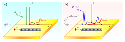
Figure 1: Comparison of non-interacting and interacting results. (a) The red curve shows host DOS with $\omega^{\nicefrac{{-1}}{{2}}}$ singularity at the band bottom, while the green curve presents the DOS for a non-interacting impurity, showing a well-defined bound state below the continuum when $\varepsilon_{d}$ is resonant with the band singularity. (b) Same as in (a), but now for an interacting impurity ($U\neq 0$). The bound state acquires a finite width, while a well-developed Kondo peak appears at the Fermi energy (see Appendix D for a critical discussion concerning the width of the bound state).

In this work, we revisit a situation similar to the last system [31], using the NRG method. To better understand the system here, we first study the non-interacting regime. In the Appendix, we discuss in detail what happens when a non-interacting resonant level (RL), generically called an impurity, is placed near (or at) the $\omega^{\nicefrac{{-1}}{{2}}}$ singularity that occurs naturally in a 1D quantum wire host (see Fig. 1(a) for an illustration). We show that the non-interacting RL spectral function, $\rho_{U=0}$ [green curve in Fig. 1(a)], exhibits a bound state below the bottom of the band DOS, $\rho_{band}$ (red curve). The bound state has the properties of a Dirac delta function (see Appendix) and carries a spectral weight that depends on the coupling of the RL to the band and its distance to the singularity in $\rho_{band}$ [visible as a sharp red peak in Fig. 1(a)]. Our results show a couple of interesting features of this deceptively simple non-interacting problem. First, there is a bound state even when the RL is positioned close to the center of the band. In that case, the bound state appears exactly at the edge of the band but carries negligible spectral weight, even for moderate coupling to the band (see discussion around Fig. 13 in the Appendix). Second, if the RL is positioned at the singularity, the bound state carries a spectral weight that is exactly $\nicefrac{{2}}{{3}}$ [34], irrespective of the coupling-strength of the RL to the band.

Once the Hubbard interaction $U$ is turned on [see Fig. 1(b)], we find that the usual Kondo profile of the impurity spectral function [$\rho_{NRG}$, blue curve in Fig. 1(b)] is modified. Indeed, the singularity strongly distorts the impurity’s lower Coulomb Blockade peak (CBP), which is now composed of a broadened bound state and a series of peaks. In addition, the Kondo temperature and the impurity occupancy are strongly affected when $\varepsilon_{d}$ is close to the band singularity. Both quantities tend to values closer to those fully in the Kondo regime (higher occupancy and lower $T_{K}$) even when the system is in an intermediate valence regime. This ‘reentrant’ Kondo regime can be also observed at temperatures around the local moment (LM) fixed point. Indeed, the magnetic susceptibility in the intermediate valence regime takes values similar to those in the Kondo regime at temperatures associated to the LM fixed point. This behavior, also visible in the NRG energy flow, is clearly associated to the existence of the bound state. We present NRG results and analysis to explore these interesting regimes in detail below.

The paper is organized as follows: In Sec. II, we present the Hamiltonian for the system to be analyzed, while Sec. III presents the NRG results. This section is divided into three parts: Sec. III.1 presents the dependence of the impurity spectral function (and charge occupancy) on the proximity of the impurity orbital level to the singularity at the bottom of the band. Subsection III.2 tracks how the bound state present in the non-interacting problem ($U=0$) is affected by the introduction of correlations (finite $U$). In Sec. III.3, we analyze the impurity susceptibility, as well as the impurity entropy, and verify that the correlated states caused by the presence of the singularity have a strong influence on the impurity properties close to the LM fixed point. The thermodynamic results are interpreted through an analysis of the NRG energy flow. Sec. IV presents results for an experimentally accessible system, where these effects could be observed, viz., an $N=3$ armchair graphene nanoribbon. This system has two singularities, at the bottom of the conduction and valence bands, that have an $\omega^{\nicefrac{{-1}}{{2}}}$-dependence, equal to that in a quantum wire system. Sec. V presents a discussion of the results and our conclusions. Finally, as mentioned above, in Appendices A to C, we analyze in detail the non-interacting system when the RL is close to the singularity, while in Appendix D we study the interacting (NRG) impurity spectral function to ascertain that the results in Sec. III.1 do not contain numerical artifacts.

II Model and Hamiltonian

In the following, we analyze the Kondo effect of an impurity coupled to a 1D quantum wire. We start with the quantum wire Hamiltonian

$$H_{\text{wire }}=\displaystyle{\sum_{k,\sigma}}(-2t\cos k-\mu)c_{k\sigma}^{\dagger}c_{k\sigma}$$ (1)

where $c^{\dagger}_{k\sigma}$ creates an electron with wave vector $k$ and spin $\sigma=\uparrow,\downarrow$, while $t=0.5$ is the nearest-neighbor hopping in the tight-binding chain (thus, $D=1$, the half bandwidth, is our unit of energy), and $\mu$ is the chemical potential. The Fermi energy, for different values of $\mu$, is always set at zero ($E_{F}=0$).

To study the Kondo state in this system, the wire is coupled to an Anderson impurity, which is modeled as

$$H_{\rm imp}=\sum_{\sigma}\varepsilon_{d}n_{\sigma}+Un_{\uparrow}n_{\downarrow},$$ (2)

where $d^{\dagger}_{\sigma}$ ($d_{\sigma}$) creates (annihilates) an electron with orbital energy $\varepsilon_{d}$ and spin $\sigma=\uparrow,\downarrow$, $n_{\sigma}=d^{\dagger}_{\sigma}d_{\sigma}$, and $U$ represents the Coulomb repulsion. The hybridization between the impurity and the conduction electrons is given by

$$H_{\mathrm{hyb}}=\sum_{k\sigma}\left(V_{k}d^{\dagger}_{\sigma}c_{k\sigma}+{\rm H.c.}\right),$$ (3)

where we consider the case of $V_{k}\equiv V$. The parameter $\Gamma=\pi V^{2}\rho_{band}(E_{F})$ determines the strength of the coupling of the impurity to the bath, where $\rho_{band}(E_{F})$ is the host’s DOS at the Fermi energy. To solve this problem, we use the well-known NRG Ljubljana open source code [35]. For most of the calculations, we have used the discretization parameter $\Lambda=2.0$ and kept at least 5000 states at each iteration. We also employ the so-called z-trick [36] (with $z=0.0625$, $0.125$, $\ldots$, and $1.0$, i.e., $N_{z}=16$) to remove oscillations (artifacts) in the physical quantities. The Kondo temperature was obtained through Wilson’s criterion [1], namely, the temperature for which the impurity susceptibility, multiplied by the temperature, reaches $0.07$. The thermodynamic quantities were calculated using the traditional single-shell approximation, while the dynamical quantities (spectral function) were calculated using the Density Matrix NRG approximation [37]. Finally, the single particle calculations in the main text (and in Appendix D) have used an imaginary part $\eta=10^{-6}$ to regularize the Green’s function.

III NRG results

III.1 Singularity effect on the impurity spectral function and charge occupancy

As described in the literature [25, 26, 27, 28, 29, 30], the Kondo state for Anderson-type systems [6] and highly asymmetric DOS (such as when the Fermi energy $E_{F}$ is close to a Van Hove singularity) strongly depends on model parameters. Indeed, our detailed analysis of the Kondo state for $E_{F}$ close to the 1D band-singularity [38] indicates that the impurity spectral function, impurity charge occupancy, and thermodynamic properties, are very sensitive to the interplay between $\varepsilon_{d}$, $U$, $V$, and $E_{F}$. In other words, small changes in the parameters, like the position of $E_{F}$ in relation to the singularity, strongly affect the Kondo state.

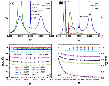
Figure 2: DOS comparison and spectral weights for $U=0$ and $U=0.01$. (a) Impurity DOS for $U=0$ ($\rho_{U=0}$, green curve) and for $\nicefrac{{U}}{{\Gamma}}=15$ ($\rho_{NRG}$, blue curve) for $\mu=0$ (when $E_{F}$ is at the center of the band, $\omega=0.0$), $U=0.01$ and $\varepsilon_{d}=\nicefrac{{-U}}{{2}}=-0.005$ (notice dashed-red-curve close to the horizontal axis, showing the band DOS, $\rho_{band}$). (b) Same as in (a), but now with $E_{F}$ very close to the singularity at the bottom of the band (depicted by the dashed red curve, $\rho_{band}$), $\mu=-0.995$, $\varepsilon_{d}=-0.005$ (right at the singularity). In (a) and (b), the $\Gamma$ value is the same for finite and vanishing $U$. (c) Finite $U=0.01$ results for the evolution of $n_{d}=\langle n_{d\uparrow}+n_{d\downarrow}\rangle$ as $E_{F}$ moves from the center of the band ($\mu=0$, right side) to very near the singularity ($\mu=-1.0-\varepsilon_{d}$, left side), for different values of $\varepsilon_{d}$ (the leftmost value of $\mu$ places the RL exactly at the singularity). The lowest (purple hexagons) curve with hexagons shows the bound state spectral weight $Z_{b}$ (see Appendix), for $U=0$ and $\varepsilon_{d}=-0.0001$. (d) Zoom of the left side of panel (c) highlighting the abrupt increase in $n_{d}$. The lowest value of the chemical potential is $\mu=-1.0-\varepsilon_{d}$, thus the curves above do not cover the same $\mu$ interval.

To reveal the most interesting aspects of the Kondo state when $\varepsilon_{d}$ is at the singularity (and $E_{F}$ is close to the bottom of the band), we will contrast it to the Kondo state obtained when $E_{F}$ is exactly in the middle of the band ($\mu=0$), keeping all the other parameters equal. We take $\varepsilon_{d}=\nicefrac{{-U}}{{2}}$, thus, for $\mu=0$ the system is in the particle-hole-symmetric (PHS) point. These results are shown in Fig. 2. Panels (a) and (b) show the impurity spectral function (green curve, for the non-interacting case, $\rho_{U=0}$, and blue curve, for the interacting case, $\rho_{NRG}$) for $\mu=0$ and $\mu=-0.995$, respectively. The (red) dashed curves are the band DOS, $\rho_{band}$. Note that all DOS results are normalized so that their integrals over $\omega$ are $1$. The parameters, kept fixed for both calculations, are $\varepsilon_{d}=-0.005$, $U=0.01$, and $\Gamma=6.6667\times 10^{-4}$ (thus $\nicefrac{{U}}{{\Gamma}}=15$). We have used $V$ values for both calculations ($V=0.026$ and $V=0.0082$, for panels (a) and (b), respectively) such that $\Gamma$ does not vary. The only change from one calculation to the other is the PH asymmetry around $E_{F}$: no asymmetry in panel (a) and a very strong asymmetry in panel (b). Comparison of the $\rho_{NRG}$ results (blue curves) in panels (a) and (b) shows how strongly the singularity affects the impurity spectral density [39]. Indeed, from a traditional PHS Kondo peak at $\mu=0$ [panel (a), blue curve], we move to a very rich impurity DOS when $\varepsilon_{d}$ is at the singularity, showing a series of peaks around the Fermi energy ($E_{F}=0.0$). The rightmost peak in $\rho_{NRG}$ (the upper CBP), farthest from the singularity, is the least affected, while the Kondo peak (around $\omega=0.0$) acquires a slight asymmetry. Notice that the RL results (green curve, $\rho_{U=0}$) show that the singularity splits the non-interacting DOS into a Dirac delta-like bound state (below the bottom of the band) and a broad peak starting at the bottom of the band. As it turns out, this last peak becomes a superposition of three peaks in the continuum, while the bound state splits into two features below the band. One is very sharp, located at the band edge, and has very small spectral weight. The other, containing most of the spectral weight, is shifted to lower energy than the original bound state, and acquires a sizable finite width [40]. Thus, the interplay between the singularity and correlations results in very complex spectral behavior. This will be further analyzed in the next subsection, III.2.

Fig. 2(c) shows how the impurity occupancy $n_{d}=\langle n_{d\uparrow}+n_{d\downarrow}\rangle$ (for $U=0.01$ and $\nicefrac{{U}}{{\Gamma}}=15$) varies when the Fermi energy moves from the center of the band ($\mu=0$) to close to the bottom of the band ($\mu=-1.0-\varepsilon_{d}$), for different values of $\varepsilon_{d}$ ($-0.005\leq\varepsilon_{d}\leq-0.0001$). Fig. 2(d) shows a zoom of the results in panel (c) close to the lowest values of $\mu$. Notice that the red squares curve at the top for $\varepsilon_{d}=-0.005$ is at the PHS point for $\mu=0$, and the occupancy is pinned at $n_{d}=1$ even as $\mu$ moves away from PHS. As expected, the average value of $n_{d}$ decreases (from $n_{d}\approx 1.0$ to $n_{d}\approx 0.45$) as $\varepsilon_{d}$ increases, from $\varepsilon_{d}=\nicefrac{{-U}}{{2}}=-0.005$ (red squares) to very close to the Fermi energy$,\varepsilon_{d}=-0.0001$ (light green left-triangles), moving the system from deep into the Kondo regime to an intermediate valence regime, even for $\mu=0$. However, as the Fermi energy approaches the bottom of the band ($\mu\approx-1.0-\varepsilon_{d}$), $n_{d}$ increases abruptly, with a faster rate the closer $\varepsilon_{d}$ is to zero.

The variation of the bound state spectral weight $Z_{b}$ [41] [purple hexagons curve in Fig. 2(c)] with $\mu$, for the non-interacting case, indicates that once the system moves to the intermediate valence regime (larger values of $\varepsilon_{d}$), the presence of the bound state below the bottom of the band, with stronger spectral weight, strongly increases the charging of the impurity. This effect is negligible if the system is well into the Kondo regime ($\varepsilon_{d}=-0.005$, red squares) or close to it ($\varepsilon_{d}\lesssim-0.003$).

As $n_{d}$ tends to approach its Kondo-value of $n_{d}\approx 1.0$, despite $\varepsilon_{d}$ approaching the intermediate valence regime, close to the bottom of the band, it is reasonable to expect that the Kondo temperature $T_{K}$ will be strongly affected. We expect $T_{K}$ will tend to return to its Kondo-value when we approach the bottom of the band in the intermediate valence regime. Indeed, this can be seen in Fig. 3(a), showing a color map of the Kondo temperature $T_{K}$ for all the points in Fig. 2(c). Focusing on the right side of the figure ($\mu=0$, $E_{F}$ at the center of the band), we see the usual increase in $T_{K}$ as we move from top to bottom (from the Kondo to the intermediate valence regime). However, looking at the bottom of the figure, moving from right to left (from center to bottom of the band) we see that $T_{K}$ decreases abruptly as we approach the bottom of the band, tending back to its low Kondo-regime value. Figure 3(b) shows a comparison of results for $T_{K}$ vs $\mu$ for different $\varepsilon_{d}=-1\times 10^{-4}$ (magenta triangles, intermediate valence regime), $\varepsilon_{d}=-1\times 10^{-3}$ (orange squares, border between Kondo and intermediate valence regimes), and $\varepsilon_{d}=-5\times 10^{-3}$ (blue circles, Kondo regime), highlighting the sharp drop in $T_{K}$ as $\mu$ approaches the singularity, when the system is in the intermediate valence regime (magenta triangles) or in a region in between Kondo and intermediate valence [42] (orange squares). This contrasts the stable behavior of $T_{K}$ when the system is deep into the Kondo regime (blue circles). Figure 3(c) shows a zoom of the results close to the singularity. Indeed, the formation of the bound state close to the Fermi energy seems to bring the system back to a Kondo regime [43].

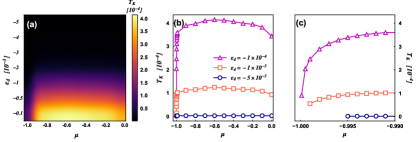
Figure 3: (a) Color map of the Kondo temperature $T_{K}$ for all the points in Fig. 2(c). The sudden drop of $T_{K}$ at the bottom left corner indicates that the bound state near $E_{F}$ moves the system back to the Kondo regime, which has a lower $T_{K}$ than in the intermediate valence regime (bottom right corner). (b) Comparison of $T_{K}$ vs $\mu$ results for $\varepsilon_{d}=-1\times 10^{-4}$ (magenta triangles, intermediate valence regime), $\varepsilon_{d}=-1\times 10^{-3}$ (orange squares, border between Kondo and intermediate valence regimes), and $\varepsilon_{d}=-5\times 10^{-3}$ (blue circles, deep into Kondo regime). (c) Zoom of the results in panel (b) close to the bottom of the band.

III.2 Evolution of the bound state with correlations

With the objective of understanding the origin of the split peaks around the singularity visible in Fig. 2(b), we present in Fig. 4 the evolution of the interacting impurity spectral function as $U$ decreases, keeping $\Gamma=8.334\times 10^{-4}$, $\varepsilon_{d}=\nicefrac{{-U}}{{2}}$, and varying $\mu$ so that, for all panels, $\varepsilon_{d}$ is at the singularity ($\mu=-1-\varepsilon_{d}$). Panels (a) to (f) show results for $\nicefrac{{U}}{{\Gamma}}=12.0$, $9.0$, $6.0$, $3.0$, $0.5$, and $0.001$, respectively ( as indicated in each panel). With decreasing $U$, the upper CBP moves to lower energy, eventually merging with a considerably broader Kondo peak, [panel (c)], resulting from the system having entered an intermediate valence regime [43]. We now focus our attention on the two peaks below the bottom of the band, whose position and spectral weight can be followed more accurately [peaks $P_{0}$ and $P_{1}$]. For decreasing $\nicefrac{{U}}{{\Gamma}}$, the leftmost peak, $P_{0}$, transfers its spectral weight to peak $P_{1}$, located at the bottom of the band. Indeed, for $\nicefrac{{U}}{{\Gamma}}\lesssim 0.5$ [panel (e)], $P_{0}$ has transferred almost all of its spectral weight to $P_{1}$, while in the interval $3\lesssim\nicefrac{{U}}{{\Gamma}}\lesssim 6$, peak $P_{0}$ splits into two peaks. For $\nicefrac{{U}}{{\Gamma}}\approx 9.0$, $P_{1}$ detaches from the bottom of the band, moving away from it for smaller $U$, while its spectral weight increases at the expense of $P_{0}$. Panel (f), for $\nicefrac{{U}}{{\Gamma}}=0.001$, has a comparison of the NRG (blue curve) and $U=0$ results [44] (dashed green curve), showing that they are virtually the same. This demonstrates that the NRG spectral function results reproduce faithfully the evolution of the many-body processes that give origin to the split peaks around the singularity, deep into the Kondo regime (panel (a), $\nicefrac{{U}}{{\Gamma}}=12$).

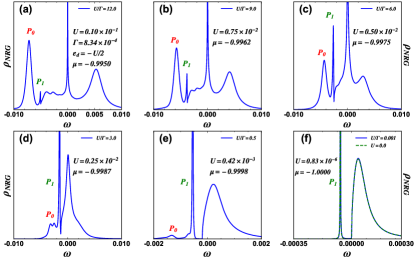
Figure 4: Evolution of the interacting impurity spectral density $\rho_{NRG}$ (blue curves), for $\Gamma=8.34\times 10^{-4}$, $\varepsilon_{d}=\nicefrac{{-U}}{{2}}$, and $\mu=-1.0-\varepsilon_{d}$, as $U$ varies from $\nicefrac{{U}}{{\Gamma}}=12$ [panel (a)] to $0.001$ [panel (f)]. The value of $\mu$ places $\varepsilon_{d}$ at the singularity in all panels. The dashed green curve in panel (f) is the non-interacting $\rho_{U=0}$ spectral function, showing excellent agreement with the $U\approx 0$ NRG result. The peaks $P_{0}$ and $P_{1}$ are associated with the bound state seen in $\rho_{U=0}$ (see text).

We now analyze $\rho_{NRG}$ in more detail in panels (a) and (b), where we still have strong correlations. In both panels, a well formed Kondo peak and an upper CBP are clearly visible. For $\nicefrac{{U}}{{\Gamma}}=9$, at energies below the Kondo peak (but still inside the continuum), a structure with two features is clearly visible. For $\nicefrac{{U}}{{\Gamma}}=12$, the Kondo peak and the upper CBP are clearly consolidated and further structure (a third smooth feature) emerges between the Kondo peak and the bottom of the band. In Appendix D, we will show that all these features (including $P_{0}$ and $P_{1}$) are not NRG numerical artifacts.

Fig. 5 presents the spectral weight [panel (a)] and position [panel (b)], in relation to the bottom of the band, of peaks $P_{0}$ and $P_{1}$ for different values in the interval $0.001\leq\nicefrac{{U}}{{\Gamma}}\leq 12.0$. In panel (b), we also plot the position of the non-interacting bound-state (blue circles), for $U=0$ and same $\varepsilon_{d}$ and $V$ values used in the NRG calculations (note that the non-interacting results depend on $\nicefrac{{-\varepsilon_{d}}}{{\Gamma}}$, which labels the upper horizontal axes in panel (b) and its inset). Following the spectral weight curves for peaks $P_{0}$ (green squares) and $P_{1}$ (red right-triangles), in Fig. 5(a), we see that, when $\nicefrac{{U}}{{\Gamma}}$ decreases from $12$ to $0.5$, the spectral weight of $P_{0}$ is almost all transferred to $P_{1}$ (although part of $P_{0}$’s spectral weight is also transferred to the continuum, and then, with further decrease of $\nicefrac{{U}}{{\Gamma}}$, to peak $P_{1}$). In the interval $0.5\geq\nicefrac{{U}}{{\Gamma}}\geq 0.001$, $P_{1}$ quickly acquires spectral weight from inside the continuum, reaching $\approx\nicefrac{{2}}{{3}}$ for very small values of $\nicefrac{{U}}{{\Gamma}}$, as expected. The inset in Fig. 5(a), shows $P_{1}$’s spectral weight in a $\log$ scale to emphasize the formation of a $\nicefrac{{2}}{{3}}$ plateau as $U\rightarrow 0$.

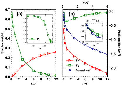
Figure 5: (a) Spectral weight, as a function of $\nicefrac{{U}}{{\Gamma}}$, for peak $P_{0}$ (red right-triangles) and peak $P_{1}$ (green squares), as defined in the discussion of Fig. 4. The inset shows $P_{1}$ spectral weight in a $\log$ scale, highlighting the $\nicefrac{{2}}{{3}}$ plateau for vanishing $U$. (b) Energy position, in relation to the bottom of the band, of $P_{0}$ (red right-triangles), $P_{1}$ (green squares), and the non-interacting bound-state (blue circles). The inset shows the exact agreement between $P_{1}$ and the bound-state positions for the smallest values of $U$. Note that the non-interacting ($U=0$) bound-state results (blue circles) are dependent on $\nicefrac{{-\varepsilon_{d}}}{{\Gamma}}$ (upper horizontal axes in the main panel and its inset), with $\varepsilon_{d}=\nicefrac{{-U}}{{2}}$, where the $U$ and $V$ values are defined by the NRG results.

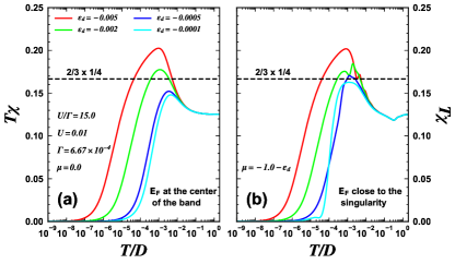
Figure 6: Impurity magnetic susceptibility $\chi$ (as a function of temperature, in units of $D$, half bandwidth), for some of the $\varepsilon_{d}$ values in Fig. 2 (d). In panel (a), the Fermi energy is fixed at the center of the band and, as $\varepsilon_{d}$ gradually increases, the system moves into the intermediate valence regime. Note that for $\varepsilon_{d}=-0.005$, the system is in the PHS point. (b) Same as in (a), but now the chemical potential is such that $\varepsilon_{d}$ remains fixed at the singularity and it is the Fermi energy that moves closer to the bottom of the band, thus $\mu=-1.0-\varepsilon_{d}$. The values of $\Gamma$ and $U$ are the same as in Fig. 2 for all calculations.

Figure 5(b) shows the evolution of the position of $P_{0}$ (red right-triangle) and $P_{1}$ (green squares), measured in relation to the bottom of the band. Their variation in position is contrasted to that of the non-interacting bound-state (blue circles). Starting from $\nicefrac{{U}}{{\Gamma}}=12$, $P_{1}$ (green squares) moves away from the bottom of the band as $\nicefrac{{U}}{{\Gamma}}$ decreases, until, at $\nicefrac{{U}}{{\Gamma}}\approx 1$, it reverses course and starts to approach the bottom of the band again. The position of $P_{1}$, the dominant peak for small values of $U$, progressively approaches the position of the bound-state, until they coincide for the two smallest values of $U$, as emphasized in the inset. Peak $P_{0}$, on the other hand, monotonically approaches the bottom of the band as $\nicefrac{{U}}{{\Gamma}}$ decreases, initially linearly, but then, around the same region where $P_{1}$ reverses course, starts to show a faster rate of approach to the bottom of the band as a function of $\nicefrac{{U}}{{\Gamma}}$. Note that, to simplify the presentation, even after $P_{0}$ split into two peaks, we are considering it as a single peak and taking a point halfway between the split peaks as $P_{0}$’s position.

Finally, the results for the position of $P_{1}$ [red right-triangles in panel (b)] can be interpreted in the following way. As $U$ decreases at fixed $\Gamma$, the Fermi energy approaches the bottom of the band, since $\epsilon_{d}=\nicefrac{{-U}}{{2}}$ is at the singularity. Since the Kondo peak becomes broader (as $\nicefrac{{U}}{{\Gamma}}$ decreases), $P_{1}$ is initially slowly forced away from the bottom of the band. However, for very small $U$ values ($\nicefrac{{U}}{{\Gamma}}\lesssim 1$), the Fermi energy gets very close to the singularity, and, since $\Gamma=\pi\rho_{0}V^{2}$ is fixed, $V$ decreases (since $\rho_{0}$ increases), and $P_{1}$, which has become the bound-state (check comparison with blue circles curve in the inset), approaches the bottom of the band again (check also $\epsilon_{b}$ in Fig. 15).

III.3 Thermodynamic properties: the fractional local moment

Figure 6 shows the impurity magnetic susceptibility for four values of $\varepsilon_{d}$ ($-0.005$, $-0.002$, $-0.0005$, and $-0.0001$). In panel (a), the Fermi energy is fixed at the center of the band ($\mu=0$) and the system stays in a more standard Kondo regime. In contrast, in panel (b), $\mu=-1.0-\varepsilon_{d}$, $E_{F}$ is located close to the bottom of the band, such that $\varepsilon_{d}$ is at the singularity for all cases. Starting at the PHS point $\varepsilon_{d}=-0.005$ [red curve, panel (a)], the system progressively moves into the intermediate valence regime as $\varepsilon_{d}$ increases ($\varepsilon_{d}$ approaches the Fermi level). As expected, the broad peak around $T\approx 0.001<<U=0.01$, seen in the red curve, is indicative of the LM fixed point. As $\varepsilon_{d}$ moves closer to the Fermi energy, charge fluctuations become more prominent, suppressing the formation of a LM at the impurity (cyan curve). On panel (b), however, where $\varepsilon_{d}$ is at the singularity, and the Fermi energy progressively approaches it, the picture that emerges is substantially different. Although there is little difference between both panels for $\varepsilon_{d}=-0.005$ (red curves), once the Fermi energy approaches $\varepsilon_{d}$, the suppression of the LM peak seems to be arrested in panel (b). The LM peak in $\chi$ stays pinned close to the $\nicefrac{{2}}{{3}}\times\nicefrac{{1}}{{4}}$ value, indicative of the presence of the bound state with spectral weight $Z_{b}=\nicefrac{{2}}{{3}}$ (see Appendix), even as $\varepsilon_{d}$ changes by an order of magnitude.

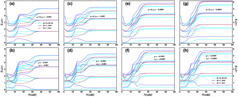
Figure 7: NRG energy flow (for odd values of N) for the same parameters as in Fig. 6. The $\varepsilon_{d}$ values, from left to right, are: $-0.005$, $-0.002$, $-0.0005$, and $-0.0001$. Top panels correspond to the Fermi energy at the center of the band; lower panels correspond to a Fermi energy close to the bottom of the band (with $\varepsilon_{d}$ at the singularity). Q is the charge in the system, measured in relation to half-filling, while $S$ indicates the total spin (see Ref. [11] for details). The parameter values for $U$ and $\Gamma$ are the same as in Fig. 6. For these NRG calculations, in particular, we have used $\Lambda=2.5$.

The behavior of $\chi$ shown in Fig. 6(b) suggests that the existence of the bound state makes the LM impervious to charge fluctuations. This is corroborated by the NRG energy flows, as shown in Fig. 7, for the same parameters as in Fig. 6. It is well-known that the three SIAM fixed points are associated to energy plateaus in the spectra as the number of NRG iterations varies. The Free Orbital, Local Moment, and Strong Coupling fixed points are successively approached as $N$ increases (which corresponds to a decrease in temperature, or energy scale behavior). This can be easily spotted in Fig. 7(a), corresponding to the PHS point, see Refs. [2, 11] for comparison. In the upper-row panels (Fermi energy at the center of the band, $\mu=0$), we see that the plateaus starting at approximately $N=10$ [Fig. 7(b)] are gradually erased as charge fluctuations increase [panels (c), (e), and (g)]. For example, in Fig. 7(g), the lowest energy state with $Q=1$ and $S=0$ (dashed blue curve) transitions directly (around $N=10$) from a high-temperature value to a low-temperature value without going through an intermediate stage. This does not happen for the lower-row panels ($E_{F}$ close to the bottom of the band). The plateau present in Fig. 7(b) (between $N=10$ and $N=30$) is still present in panel (h) (although it now finishes at around $N=20$). This is consistent with the results for a robust Kondo state seen in the impurity magnetic susceptibility in Fig. 6.

For completeness, Fig. 8 shows the impurity entropy as a function of $\nicefrac{{T}}{{D}}$, for the same parameters as in Fig. 6. We note in panel (a) ($E_{F}$ at the center of the band), for $\varepsilon_{d}=-0.005$ (red curve), the usual evolution. As temperature decreases, the impurity entropy goes from the Free Orbital ($\ln 4$) plateau, to the Local Moment ($\ln 2$) plateau, until it reaches the Strong Coupling ($\ln 1$) Kondo limit. Panel (b) shows the corresponding results when the Fermi energy is close to the bottom of the band, with $\varepsilon_{d}$ at the singularity, as in Fig. 6. We notice again a pinning tendency around the Local Moment plateau as $\varepsilon_{d}$ increases, specially for $\varepsilon_{d}=-0.002$ (green curve), whose oscillation, also observed in the corresponding result in Fig. 6, may be ascribed to the many-body states that appear between the Kondo peak and the singularity [see Fig. 2(b)]. It is important to note the non-universal low-temperature behavior of the cyan curve in panel 6(b), which shows the impurity entropy being negative in the range $10^{-5}\lesssim\nicefrac{{T}}{{D}}\lesssim 10^{-4}$. This behavior (which accompanies the non-monotonic behavior of the cyan curve in $T\chi$, Fig. 6), is reminiscent of the behavior seen in other Kondo problems in the presence of a sharp singularity or discontinuity in the DOS [25, 26, 45], and is clearly most prominent here when the RL is closest to the band singularity.

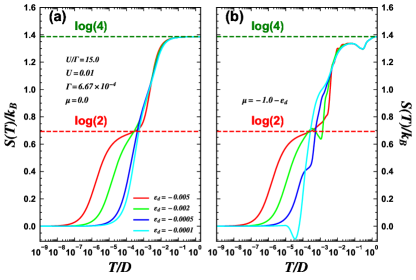
Figure 8: Impurity entropy (as a function of temperature) for the same parameters as in Fig. 6. See text for discussion of the negative values in the cyan curve in panel (b).

IV Results for an armchair graphene nanoribbon

We now discuss a possible physical implementation of the model NRG results presented in the previous sections. We study the Kondo states associated to band-edge singularities present in the DOS of an armchair graphene nanoribbon made by three carbon rows (3-AGNR), which is known to be a semiconductor [46, 47]. Such nanoribbons can be fabricated from molecular precursors [48], for example, and have been used to study Kondo resonances in experiments [49]. One interesting recent study is that of subgap states in a Kondo regime [50]. Figure 9(a) shows the DOS of an undoped 3-AGNR with symmetric valence and conduction bands. The Fermi energy can in principle be gated down until it is close to the bottom singularity of the valence band (leftmost vertical dashed line), or we may gate-dope it with slightly more electrons and bring the Fermi energy just above the bottom singularity of the conduction band (rightmost vertical dashed line). Both cases reproduce the situation studied in the previous sections, for the quantum wire. Figure 9(b) compares the $\omega$-dependence of these two singularities with that of the quantum wire, showing that they are virtually the same. Notice that panel (b) shows the hybridization function $\Delta(\omega)=\pi V^{2}\rho(\omega)$, such that $\Gamma=\pi V^{2}\rho(0)$ is the same for all three cases [51]. These results in Fig. 9(b) imply that the NRG results for the 3-AGNR and the quantum wire should be very similar. Indeed, the finite-$U$ impurity spectral function [same parameters as in Fig. 2(b)], shown in Fig. 9(c), for the conduction band singularity, is quantitatively similar to the quantum wire results in Fig. 2(b). The same occurs for the valence band singularity [Fig. 9(d)] [52].

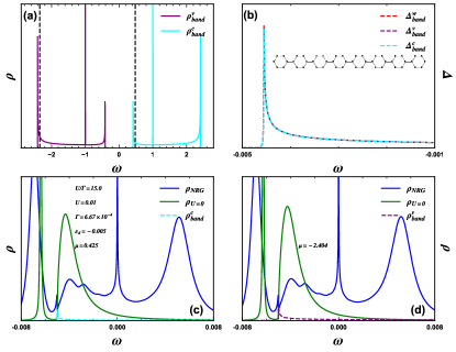
Figure 9: (a) 3-AGNR DOS, showing the very symmetric valence (purple curve) and conduction (cyan) bands. The vertical black dashed lines indicate the approximate position of the Fermi energy for the calculations in panels (c) and (d). (b) Comparison of the quantum wire singularity ($\Delta_{band}^{w}$, dashed red curve) with the 3-AGNR valence ($\Delta_{band}^{v}$, dashed purple) and conduction ($\Delta_{band}^{c}$, dashed cyan) hybridization functions lower singularities, showing they are identical. The inset shows a sketch of the 3-AGNR system. (c) Impurity DOS (blue curve, $\rho_{NRG}$) when $\varepsilon_{d}$ is at the singularity at the bottom of the conduction band. The result is very similar to Fig. 2(b), for the quantum wire singularity. (d) Same as in (c), but now $\varepsilon_{d}$ is at the valence band singularity. Also similar to panel (c). Parameter values (except for $\mu$) are as in Fig. 2(b).

V Summary, Discussion, and conclusions

We have analyzed the effect of Van Hove singularities near the Fermi energy and a magnetic impurity on the Kondo effect. Such singularities are present at the band edges of a quantum wire and of different AGNRs. The singularities present at the bottom of the valence and conduction bands of a 3-AGNR result in effective hybridization functions (at fixed $\Gamma$) with an $\omega^{\nicefrac{{-1}}{{2}}}$ dependence. Thus the spectral functions of the magnetic impurity are quantitatively similar to those obtained for a quantum wire and provide a convenient physical implementation of our model calculations [53, 48, 49]. The main results we obtained are as follows. For a non-interacting impurity, we have characterized a Dirac delta bound state below the band minimum, with properties that depend on the near-resonance of $\varepsilon_{d}$ with the singularity, and on the coupling of the impurity to the band. As expected, the larger the coupling and the closer $\varepsilon_{d}$ is to the singularity, the larger is the spectral weight $Z_{b}$ of the bound state and the farther it is below the band-minimum. The spectral weight $Z_{b}$ is vanishingly small if $\varepsilon_{d}$ is not close to the singularity, while it quickly increases as it approaches, reaching the value $Z_{b}=\nicefrac{{2}}{{3}}$ at resonance, in agreement with previous work [31], where the singularity is due to spin-orbit interaction. In addition, the impurity level $\varepsilon_{d}$ is slightly renormalized upwards due to its interaction with the singularity (see Figs. 15, 18, and 20 in the Appendix).

Once the Hubbard $U$ is present, we see several interesting effects. First, starting with the Fermi energy at the PHS point in the middle of the band [Fig. 2(a)] and then moving to the bottom of the band [Fig. 2(b)], at fixed $U$ and $\Gamma$, we see that the non-interacting bound state acquires a finite width [40] and moves further away from the bottom of the band; in addition, a discontinuity appears in the impurity DOS at the band edge. Additional structure in the spectral function appears between this discontinuity and the Kondo peak, which, aside from acquiring some asymmetry, it is barely affected. An analysis of the evolution of the impurity DOS as $U$ decreases, at fixed $\Gamma$, from $\nicefrac{{U}}{{\Gamma}}=12$ to $10^{-3}$ (see Fig. 4) allows us to follow the evolution of these many-body-related features, until the $\nicefrac{{U}}{{\Gamma}}=10^{-3}$ results match perfectly the $\nicefrac{{U}}{{\Gamma}}=0$ results.

An analysis of how the impurity is discharged as $\varepsilon_{d}$ moves closer to the Fermi energy, starting at the PHS point, shows that there is a great difference in the results for $\varepsilon_{d}$ being far from the singularity or close to the singularity. We see in Fig. 2(c) that the approach of $\varepsilon_{d}$ to the singularity ‘recharges’ the impurity, with the effect being more dramatic as it moves into the intermediate valence regime. This unusual behavior is clearly associated to the existence of the bound state. The Kondo temperature $T_{K}$ [see Fig. 3(a)], for the same set of parameters, suffers a sizeable decrease (if in the intermediate valence regime, with $E_{F}$ at the center of the band) when $E_{F}$ moves closer to the singularity at the bottom of the band. Both results, on the occupancy of the impurity and its $T_{K}$ value, show that the system partially recovers its strong coupling regime properties, i.e., higher occupancy and lower $T_{K}$, once the presence of the singularity is felt at the intermediate valence regime. This occurs because of the formation of the bound state.

In addition, the magnetic susceptibility shows that, for Fermi energy near the bottom of the band and in the intermediate valence regime, the LM fixed point is more resilient, as the impurity suppresses charge fluctuations. Figure 6(b) shows that the LM plateau is somewhat restored around the $\nicefrac{{2}}{{3}}\times\nicefrac{{1}}{{4}}$ value, indicating the influence of the bound state. This evolution is corroborated by an analysis of the NRG energy flow, shown in Fig. 7, as well as the impurity entropy (Fig. 8).

Appendix A Resonant level in the band continuum

We wish to understand how the proximity of a RL (an impurity with $U=0$) to the singularity at the bottom of the 1D band affects the RL spectral function. We will show that the main effect of the singularity is the formation of a bound state out of the continuum, and then we will analyze its properties.

We note that Ref. [31] discusses a bound state out of the continuum in 3D. There, however, it is necessary to add spin-orbit interaction (SOI), while we show that this is not the case in 1D. Thus, we add SOI to the Hamiltonian presented in the main text, Eq. (1), by rewriting it as

$$H_{\rm wire} =\sum_{k}\Psi^{\dagger}_{k}{\cal H}_{\rm wire}(k)\Psi_{k},$$ (4)

where $\Psi^{\dagger}_{k}=(c^{\dagger}_{k\uparrow},c^{\dagger}_{k\downarrow})$, $c^{\dagger}_{k\sigma}$ creates an electron with wave vector $k$ and spin $\sigma=\uparrow,\downarrow$, and ${\cal H}_{\rm wire}(k)$ is given by

$${\cal H}_{\rm wire}(k) = \left(-2t\cos k-\mu\right)\sigma_{0}+\left(\beta\sigma_{x}+\alpha\sigma_{y}\right)2\sin k,$$ (5)

where $\beta$ and $\alpha$ are the Dresselhaus [54] and Rashba [55] SOI, respectively, while $\sigma_{x}$ and $\sigma_{y}$ are spin Pauli matrices and $\sigma_{0}$ is the $2\times 2$ identity matrix. It can be shown [56] that the energy dispersion associated to this Hamiltonian may be written as

$$\varepsilon_{k\sigma}=-2\sqrt{t^{2}+|\gamma|^{2}}\cos\left(k-\sigma\varphi\right)-\mu,$$ (6)

where $\gamma=\beta+i\alpha$, $\varphi=\tan^{-1}\left(\nicefrac{{|\gamma|}}{{t}}\right)$, and $\sigma=\pm$. The band structure and the DOS for this Hamiltonian are studied in the next section.

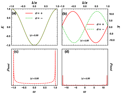
Figure 10: Band structure for $|\gamma|=0.0$ and $|\gamma|=6.0$, in panels (a) and (b), respectively. Corresponding band DOS for the same values of $|\gamma|$, in panels (c) and (d). Notice how the singularity for $|\gamma|=6.0$ [panel (d)] carries a considerably smaller spectral weight than the corresponding singularity for $|\gamma|=0.0$ [panel (c)]. Note that the range in the vertical axes in panels (c) and (d) are the same, with the integral of $\rho_{b}and$ equal to $1$ in both cases.

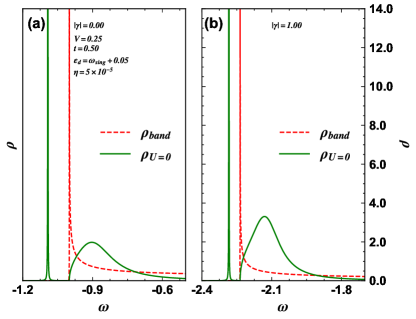
Figure 11: Band DOS $\rho_{\rm band}$ (red dashed curves) and the RL DOS $\rho_{U=0}$ (green curves) for $|\gamma|=0.0$ and $1.0$, in panels (a) and (b), respectively. The RL orbital energy $\varepsilon_{d}=\omega_{sing}+\delta$ is placed at $\delta=0.05$ above the bottom of the band $\omega_{sing}$, in both cases. In panel (a), $Z_{b}=0.554$, while in panel (b), $Z_{b}=0.415$, showing that the increase of SOI makes the bound state less bound and with a weaker spectral weight $Z_{b}$. See text for a definition of $Z_{b}$.

Appendix B Band structure and spectral function in 1D with spin orbit interaction

In this section we show that the inclusion of SOI in 1D (which already has a singularity at the bottom of the band without SOI) decreases the spectral weight of the bound state. Figure 10 shows the band structure in panels (a) ($|\gamma|=0.0$) and (b) ($|\gamma|=6.0$), with the corresponding DOS in panels (c) ($|\gamma|=0.0$) and (d) ($|\gamma|=6.0$). It is clear that SOI decreases the spectral weight carried by the singularity at the bottom of the band. This happens because a finite SOI increases the bandwidth [compare the range in the horizontal axes in Figs. 10(c) and (d)].

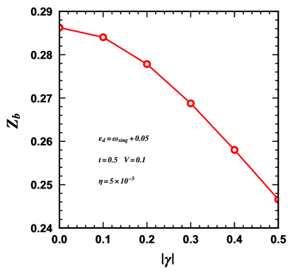
Figure 12: Variation of the bound state spectral weight $Z_{b}$ with $|\gamma|$ for $V=0.1$.

We show next that this implies a loss of spectral weight of the bound state associated with the singularity.

We calculate the RL Green’s function $\hat{G}_{imp}(\omega)$, given by

$$\hat{G}_{imp}(\omega)=\left[\left(\omega-\varepsilon_{d}\right)\sigma_{0}-\hat{\Sigma}^{(0)}(\omega)+\mathrm{i}\eta\right]^{-1},$$ (7)

where $\hat{\Sigma}^{(0)}(\omega)=\sum_{k}\hat{V}\hat{G}_{wire}(k,\omega)\hat{V}^{\dagger}$ is the hybridization self-energy, with $\hat{V}=V\sigma_{0}$, $\hat{G}_{wire}(k,\omega)=\left[\omega\sigma_{0}-{\cal H}_{wire}(k)\right]^{-1}$ is the quantum wire Green’s function, while $V$ is defined right after Eq. (3) in the main text. The RL spectral function, i.e., its DOS, is calculated through (notation as in the main text) $\rho_{U=0}(\omega)=-\frac{1}{\pi}{\rm Im\,}\mathrm{Tr}\,\hat{G}_{imp}(\omega)$.

A comparison of both the 1D lattice DOS (red curves) and the RL DOS (green curves) is shown in Fig. 11 for $|\gamma|=0.0$ and $|\gamma|=1.0$, panels (a) and (b), respectively, where we have set $\varepsilon_{d}=\omega_{sing}+\delta$ (where $\delta=0.05$ and $\omega_{sing}$ is the energy at the bottom of the band, with the band being symmetric around $\omega=0.0$), and $V=0.25$. A comparison of the RL DOS in both panels shows that a finite SOI decreases the spectral weight of the bound state [thus the area of the DOS inside the continuum in panel (b) is clearly larger than in panel (a)]. This is further detailed in what follows.

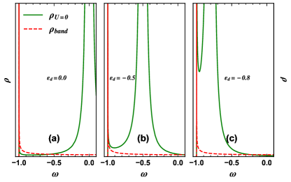
Figure 13: Resonant level DOS $\rho_{U=0}$ (green curve) for three different positions of the RL, $\varepsilon_{d}=0.0$, $-0.5$, and $-0.8$, in panels (a), (b), and (c), respectively. Notice the large increase of the spectral weight of the peak at the band singularity (red curve) as $\varepsilon_{d}$ approaches the bottom of the band. $V=0.15$ in all panels.

In Fig. 12, we show results for $Z_{b}$, which is defined as

$$Z_{b}=\int_{-\infty}^{\omega_{sing}}\rho_{U=0}(\omega)d\omega,$$ (8)

for the interval $0.0\leq|\gamma|\leq 0.5$, where $\omega_{sing}$ is the position of the singularity. It clearly shows that $Z_{b}$ decreases monotonically with $|\gamma|$. This can be understood by analyzing the $\rho_{band}$ results in Fig. 10, where we can easily see that for $|\gamma|=6.0$ there is considerably less spectral weight at the bottom of the band than for $|\gamma|=0$. Indeed, integrating $\rho_{band}$ from $\omega_{sing}$ to $\omega_{sing}+0.05$ we obtain $\approx 0.09$ for $|\gamma|=0$ and $0.04$ for $|\gamma|=6.0$. Thus, one expects that the RL will be less affected by the singularity for finite SOI. Again, this occurs because a finite SOI increases the bandwidth.

We have established that the presence of SOI in 1D weakens both the band-edge singularity and the resulting bound state. This is in contrast to the 3D system in [31] that requires SOI to create a singular DOS. In what follows we analyze the properties of the 1D system without SOI.

Figure 14: (a) Variation of the RL DOS $\rho_{U=0}$ with the coupling to the band in the interval $0.005\leq V\leq 0.2$, for $|\gamma|=0.0$ and $\delta=0.05$. (b) The variation of $Z_{b}$ for $0.01\leq V\leq 0.25$.

Appendix C Bound state properties

C.1 Bound state and coupling to the band

First, we find that no matter what the energy of the RL is in relation to the singularity, there is always a bound state located either at the singularity or below it [44]. The latter occurs when the coupling of the RL to the band is strong, or if the RL is close to the singularity. In Fig. 13, we show the RL DOS, $\rho_{U=0}$, for three different positions of the RL in relation to the bottom of the band. In panel (a), the RL is located at the center of the band, $\varepsilon_{d}=0$, and the singularity is at $\omega=-1.0$. We notice a vanishingly narrow DOS peak at the singularity. In panel (b), the RL is located at $\varepsilon_{d}=-0.5$, midway between the center of the band and the singularity. The DOS peak at the singularity has increased considerably. Finally, when the RL is just $0.2$ above the singularity, $\varepsilon_{d}=-0.8$, the bound state spectral weight at the singularity has increased drastically. If the coupling increases, and/or the RL approaches the singularity even more, the bound state detaches from the band continuum and moves to lower energies, as will be seen below.

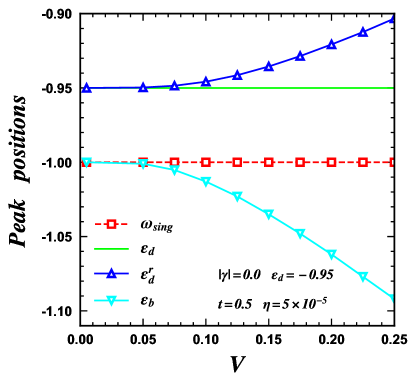
Figure 15: Analysis of the formation of the bound state in the RL spectral function $\rho_{U=0}$, as a function of $V$ [obtained from the results in Fig. 14(a)]. Red curve shows the bottom of the band (position of the singularity), the green curve shows the position of $\varepsilon_{d}$, the blue curve shows $\varepsilon_{d}^{r}$, the renormalized position of the RL orbital energy, while the cyan curve shows the position of the bound state, $\varepsilon_{b}$.

Fig. 14(a) shows the RL DOS as we vary its coupling to the band in the range $0.005\leq V\leq 0.2$, while keeping $\varepsilon_{d}=\omega_{sing}+0.05$. For the smallest $V=0.005$ (green curve), a bound state at the singularity is not visible (vanishingly small spectral weight). For $V=0.05$ (blue curve) a very sharp peak at the singularity is already visible (with $Z_{b}=0.044$), while for $V=0.1$ (cyan curve) the bound state has detached from the bottom of the band and moved to lower energies. Its spectral weight has also increased to $Z_{b}=0.1566$. This trend continues as $V$ increases. Figure 14(b) shows the $Z_{b}$ increase with $V$, reaching more than half of the total spectral weight for $V=0.25$.

Now, we analyze the data in Fig. 14 in more detail. Figure 15 shows how the splitting of the RL $\varepsilon_{d}$ (green circles) into two parts, one, a renormalized peak $\varepsilon_{d}^{r}$ (blue up-triangles) inside the continuum, and the bound state $\varepsilon_{b}$ (magenta down-triangles), below the bottom of the band, progresses as one increases $V$. The red squares mark the bottom of the band.

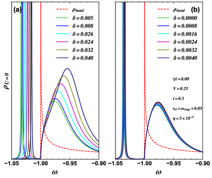
Figure 16: Panels (a) and (b) show the variation of $\rho_{U=0}$ with $\delta$ ($\varepsilon_{d}$ offset from the bottom of the band) for two different intervals: (a) $0.005\leq\delta\leq 0.04$ and (b) $0.0005\leq\delta\leq 0.004$. Panel (a) results show that, starting from $\delta=0.08$ (dark blue curve), up to $\delta=0.016$ (blue curve), changes in $Z_{b}$ and peak positions are considerable, while panel (b) results show that further approaching $\varepsilon_{d}$ from the bottom of the band ($\delta\lesssim 0.01$) has limited effects. Results obtained for $|\gamma|=0.0$ and $V=0.25$.

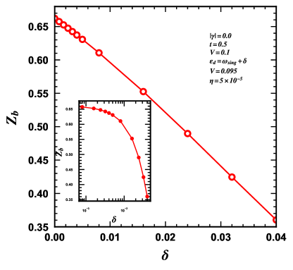
Figure 17: Variation of the bound state spectral weight $Z_{b}$ as a function of $\delta$ in the interval $0.001\leq\delta\leq 0.08$. Results obtained from both panels in Fig. 16. The inset shows the same results, but with a $\log$ scale in the $\delta$-axis, highlighting the approach to the $Z_{b}=\nicefrac{{2}}{{3}}$ value.

C.2 Bound state and distance to singularity

Now, we analyze how the bound state varies as we move the RL $\varepsilon_{d}$ closer to the singularity. We set $\varepsilon_{d}=\omega_{sing}+\delta$, where $\omega_{sing}$ marks the bottom of the band, and vary $0.0\leq\delta\leq 0.04$ (we fix $V=0.1$). The results are shown in Figs. 16(a) and (b). Once $\varepsilon_{d}$ approaches $\omega_{sing}$ ($\delta$ tends to zero), the variation is very small, i.e., $\varepsilon_{b}$ and $Z_{b}$ tend to a fixed value.

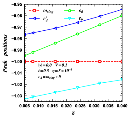
Figure 18: Similar results as in Fig. 15, but now for the variation of $\delta$. The results shown are just for panel (a) in Fig. 16.

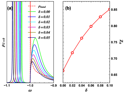
Figure 19: Similar results as in Fig 16, but now when the impurity is placed below the bottom of the band (note that $\varepsilon_{d}=\omega_{sing}-\delta$) and $V=0.1$. (a) Results for $\rho_{U=0}$, for $0.0\leq\delta\leq 0.1$, showing again the peak splitting. (b) Spectral weight $Z_{b}$ of the bound state, now larger than $\nicefrac{{2}}{{3}}$.

The variation of $Z_{b}$ with $\delta$ may be seen in Fig. 17. We see that $\delta\rightarrow 0.0$ implies $Z_{b}\rightarrow\nicefrac{{2}}{{3}}$, in agreement with the results obtained in Ref. [31]. This shows the very interesting phenomenon that the $Z_{b}=\nicefrac{{2}}{{3}}$ result does not depend on the details of the band, such as spatial dimensionality (3D vs 1D) and presence vs absence of SOI. The inset, with a $\log$ scale in the $\delta$-axis, emphasizes the gradual approach to the $Z_{b}=\nicefrac{{2}}{{3}}$ value.

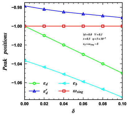
Figure 20: Similar results as in Fig. 18, but now $\varepsilon_{d}$ (green curve) is placed below the bottom of the band. Larger peak separations are obtained this way.

Figure 18 shows details of the results in Fig. 16(a), as done in Fig. 15 for the results in Fig. 14(a).

Figure 19 shows what happens when we place $\varepsilon_{d}$ out of the continuum, i.e., $\varepsilon_{d}=\omega_{sing}-\delta$ and $0.0\leq\delta\leq 0.05$, with $V=0.1$. Panel (b) shows that $Z_{b}$ takes values above $\nicefrac{{2}}{{3}}$, increasing with $\delta$. The DOS inside the continuum, as can be seen in panel (b), tends to accumulate at the bottom of the band as $\delta$ increases.

Finally, Fig. 20 shows details of the results in Fig. 19(a).

Appendix D Study of the impurity spectral function

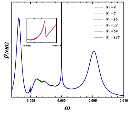
Figure 21: Analysis of the $\rho_{NRG}$ dependence on $N_{z}$ (interleaving parameter [57]) for the results in Fig. 2(b), in the interval $4\leq N_{z}\leq 128$. The inset shows a zoom in the region where the curves (except for $N_{z}=4$) vary the most (around $P_{1}$). Taking the peak-height change as a measure of the overall variation in this region, we obtain that the variation between $N_{z}=16$ and $N_{z}=8$, $N_{z}=32$ and $N_{z}=16$, $N_{z}=64$ and $N_{z}=32$, and $N_{z}=128$ and $N_{z}=64$, is $4.1$%, $1.5$%, $0.4$%, and $0.08$%, respectively. Thus, for the purpose of presentation, the results are already well-converged for $N_{z}=16$ (value used in this work). As to exposing numerical artifacts, good convergence has been achieved for $N_{z}=32$ (see text).

In this section, we follow Ref. [57] and do an step by step analysis of the results in Figs. 2 and 4, to show that the NRG spectral function features discussed in Secs. III.1 and III.2 are not numerical artifacts. There are quite a few aspects that should be taken into account to root out NRG numerical artifacts in the impurity spectral function $\rho_{NRG}$. According to Žitko and Pruschke [57], overbroadenig effects reduce energy resolution at higher energies and wash out spectral features with small spectral weight (like $P_{1}$, in Figs. 2 and 4, for the larger values of $U/\Gamma$). The so-called interleaved method (or ‘$z$ averaging’) [36] allows for the use of narrower broadening functions, mitigating overbroadening and removing oscillatory features in the impurity spectral function. The method consists of performing several ($N_{z}$) NRG calculations for different logarithmic discretization meshes and then taking their average to obtain the final impurity spectral function. However, one has to check that convergence has been attained, before trying to root out artifacts. Figure 21 shows the evolution of $\rho_{NRG}$ with increasing $N_{z}$ in the interval $4\leq N_{z}\leq 128$. It is clear that $N_{z}=4$ (green curve) is not nearly enough; however, for $N_{z}\geq 16$, $\rho_{NRG}$ has converged. It is interesting to note that $P_{1}$ is the last feature to converge. Indeed, the largest difference (which occurs around $P_{1}$, as shown in the inset) between $N_{z}=16$ and $8$ is $\approx 4.1$%, while it is $\approx 1.5$% for the difference between $N_{z}=32$ and $16$. This value falls to $\approx 0.4$% for $N_{z}=64$ (in relation to $32$), and to $\approx 0.08$% for $N_{z}=128$ (in relation to $64$). Thus, for the purpose of exposing numerical artifacts [57] (see next step), all spectral function features are well-converged for $N_{z}=32$.

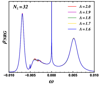
Figure 22: Analysis of the $\Lambda$ dependence of the $\rho_{NRG}$ results in Fig. 2(b) in the interval $1.6\leq\Lambda\leq 2$. As shown in Ref. [57], NRG discretization artifacts should shift position and change form significantly with decreasing $\Lambda$. Note that we use the well-converged $N_{z}=32$ results for this analysis.

The next step, once $N_{z}$ convergence of all $\rho_{NRG}$ features has been ensured, is to analyze its dependence with $\Lambda$ (discretization parameter). Indeed, artifacts will shift (and change form) substantially when $\Lambda$ varies, while real features will change very little [57]. Usually, the detection of artifacts is more effectively done when one studies the approach to the continuum limit ($\Lambda\rightarrow 1$). Thus, we decreased the discretization parameter below the standard $\Lambda=2$ value (down to $1.6$). Figure 22 shows $\rho_{NRG}$ results for the same parameters as in Fig. 2(b) (except that now $N_{z}=32$), for the interval $1.6\leq\Lambda\leq 2$ (varying in steps of $0.1$). It is clear that peaks $P_{0}$ and $P_{1}$, which were discussed in detail in Sec. III.2, suffer marginal changes, indicating that they are not numerical artifacts.

One last step consists in applying the so-called ‘self-energy trick’ [58] (dubbed $\Sigma$-t, for short, in Fig. 23), which is a very efficient method to reduce overbroadening effects [57]. This ‘trick’ consists in calculating the impurity self-energy as the ratio of two correlation functions, and then using it to obtain the impurity Green’s function, whose imaginary part is proportional to the impurity spectral function. It is important to remark that all our spectral function results in this work were obtained by using $\Sigma$-t. In Fig. 23, we compare our results for Fig. 4 (obtained through $\Sigma$-t, blue curves) with the results obtained without the use of $\Sigma$-t (red curves). There are some interesting points to stress. First, in all panels, the use of $\Sigma$-t results in the narrowing of some features, most notably of $P_{1}$, mainly in panels (a) and (b), where $P_{1}$ is barely noticeable without $\Sigma$-t [especially in panel (a)]. In addition, we want to call special attention to the result in panel (f), where the use of $\Sigma$-t (blue curve) has narrowed the non-$\Sigma$-t result (red curve) almost perfectly into the exact non-interacting ($U=0$) result (dashed green curve). This is emphasized in panel (f)’s inset. Since there is no reason for the accuracy of the $\Sigma$-t spectral function to be reduced for finite $U$ [58], we can have confidence in the accuracy of the spectral function results presented in Figs. 2 and 4, in the main text.

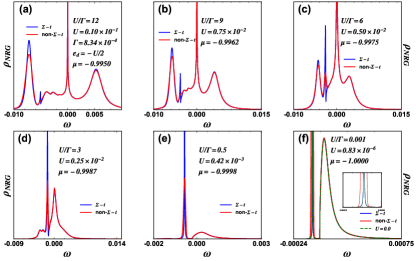
Figure 23: Reproduction of the results in Fig. 4, comparing the impurity spectral function $\rho_{NRG}$ calculated using the so-called ‘self-energy trick’ [58] (blue curves) with the results obtained without its use (red curves). The inset in panel (f) zooms in on the bound state, showing that the self-energy trick removes the overbroadening and produces the exact result (dashed green curve).

The NRG package used here (NRG Ljubljana [35]) has the so-called ‘patching procedure’ [59] fully implemented, and it was used in all spectral function calculations done here. It is well-known that the NRG is an iterative procedure which solves consecutive so-called Wilson chains with increasing sizes $N$. The energy window being analyzed, at each specific stage of the iterative procedure, logarithmically approaches the ground state region of the spectra for two consecutive iterations. One has to carefully ‘join’ (patch) the spectral information acquired at iterations $N+2$ and $N$. This procedure results in a smooth spectral function across energy windows at different energy scales.

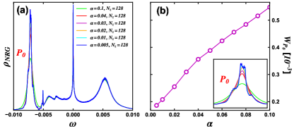
Figure 24: (a) Variation of $\rho_{NRG}$—same parameters as in Fig. 4(a), but now for $N_{z}=128$ instead of $16$—with the NRG broadening parameter $0.005\leq\alpha\leq 0.1$. (b) Half-width at half-height $W_{P_{0}}$ of the $P_{0}$ peak in panel (a) as a function of $\alpha$. The inset shows a zoom of $P_{0}$.

Finally, to analyze if the finite-width of $P_{0}$, observed in Fig. 4, is caused by NRG overbroadening, we present, in Fig. 24(a), $\rho_{NRG}$ for the same parameters as in Fig. 4(a), but now for $N_{z}=128$ (instead of 16), and varying values of the broadening NRG parameter $0.005\leq\alpha\leq 0.1$ . As shown in Fig. 21, the result for $\alpha=0.1$ (green curve) [same $\alpha$ as used in Fig. 4(a)], changes very little when we increase $N_{z}$, in this case, from $N_{z}=16$ [Fig. 4(a), blue curve] to $N_{z}=128$ [Fig. 24(a), green curve]. For decreasing $\alpha$ values, we see that the largest changes in $\rho_{NRG}$ occur for $P_{0}$ [a zoom of $P_{0}$ is shown in the inset in Fig. 24(b)]. As shown in panel (b), the $P_{0}$ half-width at half-height, denoted $W_{P_{0}}$, decreases by $67$% (from $5.5\times 10^{-4}$ to $1.8\times 10^{-4}$), while $\alpha$ decreases $20$ times (from $0.1$ to $0.05$). However, one cannot rule out the possibility that the peak width will extrapolate to zero. Thus, NRG cannot conclusively resolve this issue.

References

- Hewson [1993] A. C. Hewson, The Kondo Problem to Heavy Fermions, Cambridge Studies in Magnetism (Cambridge University Press, 1993).
- Krishna-murthy et al. [1980] H. R. Krishna-murthy, J. W. Wilkins, and K. G. Wilson, Renormalization-group approach to the Anderson model of dilute magnetic alloys. I. Static properties for the symmetric case, Phys. Rev. B 21, 1003 (1980).
- Madhavan et al. [1998] V. Madhavan, W. Chen, T. Jamneala, M. Crommie, and N. Wingreen, Tunneling into a single magnetic atom: Spectroscopic evidence of the kondo resonance, Science 280, 567 (1998).
- Goldhaber-Gordon et al. [1998] D. Goldhaber-Gordon, H. Shtrikman, D. Mahalu, D. Abusch-Magder, U. Meirav, and M. Kastner, Kondo effect in a single-electron transistor, Nature 391, 156 (1998).
- Coleman [2015] P. Coleman, Introduction to Many-Body Physics (Cambridge University Press, 2015).
- Anderson [1961] P. W. Anderson, Localized magnetic states in metals, Phys. Rev. 124, 41 (1961).
- Schrieffer and Wolff [1966] J. R. Schrieffer and P. A. Wolff, Relation between the Anderson and Kondo Hamiltonians, Phys. Rev. 149, 491 (1966).
- Kondo [1964] J. Kondo, Resistance minimum in dilute magnetic alloys, Prog. Theor. Phys. 32, 37 (1964).
- Wilson [1975] K. G. Wilson, The renormalization group: Critical phenomena and the Kondo problem, Rev. Mod. Phys. 47, 773 (1975).
- Wilson [1983] K. G. Wilson, The renormalization group and critical phenomena, Rev. Mod. Phys. 55, 583 (1983).
- Bulla et al. [2008] R. Bulla, T. A. Costi, and T. Pruschke, Numerical renormalization group method for quantum impurity systems, Rev. Mod. Phys. 80, 395 (2008).
- Vojta and Bulla [2002] M. Vojta and R. Bulla, A fractional-spin phase in the power-law Kondo model, Eur. Phys. J. B 28, 283 (2002).
- Withoff and Fradkin [1990] D. Withoff and E. Fradkin, Phase transitions in gapless Fermi systems with magnetic impurities, Phys. Rev. Lett. 64, 1835 (1990).
- Borkowski and Hirschfeld [1992] L. S. Borkowski and P. J. Hirschfeld, Kondo effect in gapless superconductors, Phys. Rev. B 46, 9274 (1992).
- Chen and Jayaprakash [1995] K. Chen and C. Jayaprakash, The Kondo effect in pseudo-gap Fermi systems: A renormalization group study, J. Phys. Condens. Matter 7, L491 (1995).
- Ingersent [1996] K. Ingersent, Behavior of magnetic impurities in gapless fermi systems, Phys. Rev. B 54, 11936 (1996).
- Bulla et al. [1997] R. Bulla, T. Pruschke, and A. C. Hewson, Anderson impurity in pseudo-gap Fermi systems, J. Phys. Condens. Matter 9, 10463 (1997).
- Gonzalez-Buxton and Ingersent [1998] C. Gonzalez-Buxton and K. Ingersent, Renormalization-group study of Anderson and Kondo impurities in gapless Fermi systems, Phys. Rev. B 57, 14254 (1998).
- Bulla et al. [2000] R. Bulla, M. T. Glossop, D. E. Logan, and T. Pruschke, The soft-gap Anderson model: Comparison of renormalization group and local moment approaches, J. Phys. Condens. Matter 12, 4899 (2000).
- Ingersent and Si [2002] K. Ingersent and Q. Si, Critical local-moment fluctuations, anomalous exponents, and scaling in the Kondo problem with a pseudogap, Phys. Rev. Lett. 89, 076403 (2002).
- Dias da Silva et al. [2009] L. G. G. V. Dias da Silva, N. Sandler, P. Simon, K. Ingersent, and S. E. Ulloa, Tunable Pseudogap Kondo Effect and Quantum Phase Transitions in Aharonov-Bohm Interferometers, Phys. Rev. Lett. 102, 166806 (2009).
- Žitko et al. [2009] R. Žitko, J. Bonča, and T. Pruschke, Van Hove singularities in the paramagnetic phase of the Hubbard model: DMFT study, Phys. Rev. B 80, 245112 (2009).
- Mitchell and Fritz [2013] A. K. Mitchell and L. Fritz, Kondo effect with diverging hybridization: Possible realization in graphene with vacancies, Phys. Rev. B 88, 075104 (2013).
- Mitchell et al. [2013] A. K. Mitchell, M. Vojta, R. Bulla, and L. Fritz, Quantum phase transitions and thermodynamics of the power-law Kondo model, Phys. Rev. B 88, 195119 (2013).
- Zhuravlev [2009] A. Zhuravlev, Negative impurity magnetic susceptibility and heat capacity in a Kondo model with narrow peaks in the local density of electron states, Phys. Metals Metallogr. 108, 107 (2009).
- Zhuravlev and Irkhin [2011] A. K. Zhuravlev and V. Y. Irkhin, Kondo effect in the presence of van Hove singularities: A numerical renormalization group study, Phys. Rev. B 84, 245111 (2011).
- Žitko and Bonča [2011] R. Žitko and J. Bonča, Kondo effect in the presence of Rashba spin-orbit interaction, Phys. Rev. B 84, 193411 (2011).
- Shchadilova et al. [2014] Y. E. Shchadilova, M. Vojta, and M. Haque, Single-impurity Kondo physics at extreme particle-hole asymmetry, Phys. Rev. B 89, 104102 (2014).
- Žitko and Horvat [2016] R. Žitko and A. Horvat, Kondo effect at low electron density and high particle-hole asymmetry in 1d, 2d, and 3d, Phys. Rev. B 94, 125138 (2016).
- Wong et al. [2016] A. Wong, S. E. Ulloa, N. Sandler, and K. Ingersent, Influence of Rashba spin-orbit coupling on the Kondo effect, Phys. Rev. B 93, 075148 (2016).
- Agarwala and Shenoy [2016] A. Agarwala and V. B. Shenoy, Quantum impurities develop fractional local moments in spin-orbit coupled systems, Phys. Rev. B 93, 241111 (2016).
- Charlier et al. [2007] J.-C. Charlier, X. Blase, and S. Roche, Electronic and transport properties of nanotubes, Rev. Mod. Phys. 79, 677 (2007).
- Wakabayashi et al. [2010] K. Wakabayashi, K. ichi Sasaki, T. Nakanishi, and T. Enoki, Electronic states of graphene nanoribbons and analytical solutions, Sci. Technol. Adv. Mater. 11, 054504 (2010).
- [34] A similar result was obtained in [31] for a 3D free-electron gas with a very strong spin-orbit interaction (SOI). That system shows an SOI-dependent singularity at the bottom of the band. The authors solve the problem in the continuum and use an energy cut-off to handle the divergence. We stress that the 1D lattice model already contains a divergence at the bottom of the band and there is no need to introduce SOI. The introduction of SOI in the 1D wire weakens the bound state, as shown in the Appendix.
- Žitko [2021] R. Žitko, NRG Ljubljana (2021).
- Campo and Oliveira [2005] V. L. Campo and L. N. Oliveira, Alternative discretization in the numerical renormalization-group method, Phys. Rev. B 72, 104432 (2005).
- Hofstetter [2000] W. Hofstetter, Generalized numerical renormalization group for dynamical quantities, Phys. Rev. Lett. 85, 1508 (2000).
- [38] The sign of the chemical potential in Eq. (1) is such that corresponds to half-filling (Fermi energy at the center of the band), and corresponds to the Fermi energy at the singularity (at the bottom of the band).
- [39] Note that the spectral weight of the bound-state (not shown) for is vanishingly small (see Appendix).
- [40] In Appendix D, we were able to show that most of the features present in the impurity spectral function are real. Although suggestive of an actual finite width for the bound state (peak ), one cannot ascertain its finite value and independence of calculation parameters.
- [41] See Eq. (B2) in the Appendix for the definition of the bound state spectral weight .
- Costi and Zlatić [2010] T. A. Costi and V. Zlatić, Thermoelectric transport through strongly correlated quantum dots, Phys. Rev. B 81, 235127 (2010).
- [43] Notice that at the bottom of Fig. 3(a) the system is in an intermediate valence regime, so that a proper Kondo temperature is not well defined. However, as will be shown in Figs. 6 and 7, the presence of the bound state strongly affects the LM fixed point of the impurity, suppressing its charge fluctuations, forcing it back into the Kondo regime.
- [44] We have checked that the bound state is a Dirac delta function, since its half-width at half-height is exactly [see Eq. (7)].
- Mastrogiuseppe et al. [2014] D. Mastrogiuseppe, A. Wong, K. Ingersent, S. E. Ulloa, and N. Sandler, Kondo effect in graphene with Rashba spin-orbit coupling, Phys. Rev. B 90, 035426 (2014).
- Lin et al. [2009] H.-H. Lin, T. Hikihara, H.-T. Jeng, B.-L. Huang, C.-Y. Mou, and X. Hu, Ferromagnetism in armchair graphene nanoribbons, Phys. Rev. B 79, 035405 (2009).
- Almeida et al. [2022] P. A. Almeida, L. S. Sousa, T. M. Schmidt, and G. B. Martins, Ferromagnetism in armchair graphene nanoribbon heterostructures, Phys. Rev. B 105, 054416 (2022).
- Cai et al. [2010] J. Cai, P. Ruffieux, R. Jaafar, M. Bieri, T. Braun, S. Blankenburg, M. Muoth, A. P. Seitsonen, M. Saleh, X. Feng, K. Muellen, and R. Fasel, Atomically precise bottom-up fabrication of graphene nanoribbons, Nature 466, 470 (2010).
- Li et al. [2017] Y. Li, A. T. Ngo, A. DiLullo, K. Z. Latt, H. Kersell, B. Fisher, P. Zapol, S. E. Ulloa, and S.-W. Hla, Anomalous Kondo resonance mediated by semiconducting graphene nanoribbons in a molecular heterostructure, Nat. Commun. 8, 10.1038/s41467-017-00881-1 (2017).
- Zalom and Žonda [2022] P. Zalom and M. Žonda, Subgap states spectroscopy in a quantum dot coupled to gapped hosts: Unified picture for superconductor and semiconductor bands, Phys. Rev. B 105, 205412 (2022).
- [51] A calculation for a 5-AGNR shows the same behavior, viz., the bottom singularities for the valence and conduction bands produce identical hybridization functions to the one for the quantum wire.
- [52] An NRG analysis for the case where is resonant with the very sharp conduction band singularity at [see Fig. 9(a)] demands a much more sophisticated discretization procedure [see, for example, R. Žitko, Comput. Phys. Commun. 180, 1271 (2009)]. We leave this problem as a subject for a future work.
- Kitao et al. [2020] T. Kitao, M. W. A. MacLean, K. Nakata, M. Takayanagi, M. Nagaoka, and T. Uemura, Scalable and precise synthesis of armchair-edge graphene nanoribbon in metal-organic framework, J. Am. Chem. Soc. 142, 5509 (2020).
- Dresselhaus [1955] G. Dresselhaus, Spin-orbit coupling effects in zinc blende structures, Phys. Rev. 100, 580 (1955).
- Bychkov and Rashba [1984] Y. A. Bychkov and E. I. Rashba, Oscillatory effects and the magnetic susceptibility of carriers in inversion layers, J. Phys. C 17, 6039 (1984).
- Lopes et al. [2020] V. Lopes, G. B. Martins, M. A. Manya, and E. Anda, V, Kondo effect under the influence of spin-orbit coupling in a quantum wire, J. Phys. Condens. Matter 32, 10.1088/1361-648X/aba45c (2020).
- Žitko and Pruschke [2009] R. Žitko and T. Pruschke, Energy resolution and discretization artifacts in the numerical renormalization group, Phys. Rev. B 79, 085106 (2009).
- Bulla et al. [1998] R. Bulla, A. C. Hewson, and T. Pruschke, Numerical renormalization group calculations for the self-energy of the impurity Anderson model, J. Phys. Condens. Matter 10, 8365 (1998).
- Bulla et al. [2001] R. Bulla, T. A. Costi, and D. Vollhardt, Finite-temperature numerical renormalization group study of the Mott transition, Phys. Rev. B 64, 045103 (2001).
- Note [1] The Gaussian broadening used, , is related to , by , where is the pole being broadened.