FORFIS: A forest fire firefighting simulation tool for education and research

Abstract

We present a forest fire firefighting simulation tool named FORFIS that is implemented in Python. Unlike other existing software, we focus on a user-friendly software interface with an easy-to-modify software engine. Our tool is published under GNU GPLv3 license and comes with a GUI as well as additional output functionality. The used wildfire model is based on the well-established approach by cellular automata in two variants – a rectangular and a hexagonal cell decomposition of the wildfire area. The model takes wind into account. In addition, our tool allows the user to easily include a customized firefighting strategy for the firefighting agents.

I Introduction

Forest fires cause widespread damage to society. In addition to ecological consequences due to the destruction of large landscapes and the loss of living space, forest fires are a great danger to all living creatures in the vicinity. The cost for firefighting and repairing the destroyed areas is enormous. Costs of more than one billion US dollars have been reported in some cases [1]. Meanwhile, the changes in weather parameters, such as temperature and soil moisture, which are occurring in the course of ongoing global warming, are favouring the spread of forest fires. It is assumed that forest fires will become more frequent [2].

Consequently, it is of great importance to optimize the strategies for fighting forest fires and to limit the damage. At the same time, the use of robotic systems to support or replace human operators is desirable to protect them from the hazards and to simplify firefighting even in difficult environmental conditions such as wind or challenging terrain.

The basis for the development or calculation of strategies is a dynamic model of a forest fire. There is a rich collection of works in the area of modelling forest fires both with the theoretical approach and the practical approach in terms of numerical computation. Among the earliest works on fire models is the one of Rothermel [3], which has been cited since now more than 3000 times. Rothermel’s approach can be categorized in models where the fire front possesses elliptical shape and travels along a continuous plane. Solutions of the dynamics of this approach are typically obtained by solving partial differential equations. In contrast, computationally simpler is the approach by cellular automata, which uses time- and state-discrete dynamics. It was first introduced by [4] with numerous other works following up [5, 6, 7, 8]. (For a survey, see [9].)

There is a large amount of software packages that implement wildfire forecasting, with some of them being available as open-source. A compact summary of various tools is given in [10]. The tools described therein, such as Phoenix [11], the popular tool FARSITE [12] or SPARK [13] provide very accurate models. However, their downside is that they must be fed with a lot of location-specific data making a spontaneous use complicated. Also, the computational complexity does not allow to use those tools for further purposes like investigating firefighting strategies. Investigating firefighting strategies on a formal level is a relatively new discipline, e.g. [14, 15, 16], which is probably due to the fact that the compute resources significantly increased in the past years.

This work introduces FORFIS, which is a forest fire simulation tool. The present work has been particularly motivated by the works [15, 16], which come with open-source implementations. Therein, a wildfire model combined with a deep reinforcement learning approach for computing a firefighting strategy are implemented.

The motivation for the development of our tool FORFIS is twofold. Firstly, it shall attract students’ attention by making modifications in the model parameters simple and understandable. Secondly, due to modular structure of the software, it can be easily modified so that research work can be performed with it. The works [15, 16] use a rectangular cellular automaton to model the wildfire dynamics. Our software additionally comes with a hexagonal cellular automaton, which leads to more accurate fire models [7]. Our tool can be cloned from

https://github.com/MBredlau/ForFiS

and run using ./main.py provided that python3 is installed.

We organize the remaining part of this article as follows. In Section II the implemented forest fire model is rigorously defined. Also, the firefighting agents model is explained. Section III describes the user interfaces.

II Forest fire and firefighting agents model

As already indicated, our work follows in part the methods in [15, 16]. More specifically, we follow the approach of cellular automata to model wildfires and the firefighting agents act on that model. The wildfire model and the agents model are discussed in Section II-B and Section II-C, respectively. In Section II-A basic notation and concepts required subsequently are introduced.

II-A Preliminaries

The symbols $\mathbb{N}$ and $\mathbb{R}$ stand for the set of positive integers and the set of real numbers, respectively. If $M$ is a set and $N\in\mathbb{N}$ then $M^{N}$ stands for the $N$-fold Cartesian product of $M$, e.g. $M^{2}=M\times M$. The notation $f\colon A\rightrightarrows B$ stands for a set-valued map with domain $A$ and as image subsets of $B$. $f$ is strict if $f(a)\neq\emptyset$ for all $a\in A$.

The next definition is crucial for the present work as it allows to model the forest fire and the firefighting agents in a simple and concise form.

Definition II.1

A transition system is a triple

$$(X,U,F)$$ (1)

where $X$ and $U$ are non-empty sets and $F\colon X\times U\rightrightarrows X$ is a strict set-valued map. The components of (1) are called state space, input space and transition function, respectively.

A transition system (1) is implicitly equipped with time-discrete dynamics of the form

$$x(t+1)\in F(x(t),u(t)).$$ (2)

The use of a differential inclusion allows to model uncertainties in the dynamics. Thereafter, we will model a forest fire by a transition system where the transition function is modelled by probabilities so that the forest fire model is basically a Markov decision process.

II-B Forest fire model

To model the wildfire, we use a special transition system of the form (1). Firefighting agents have an impact on the wildfire by the input of this transition system. In brief, we subdivide the forest area, which is assumed to be two-dimensional, flat and compact, into $N\in\mathbb{N}$ sub-areas. Formally, we define a finite partition on the forest area and the topological closures of the elements of this partition are congruent to each other. See Fig. 1(a).

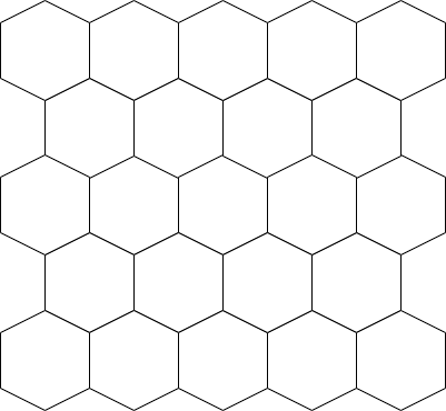
(a)

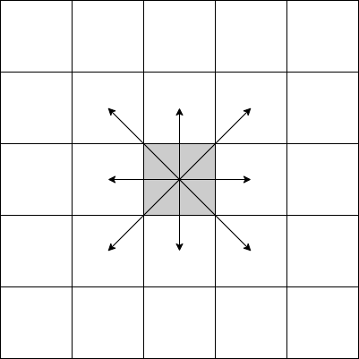
(b)

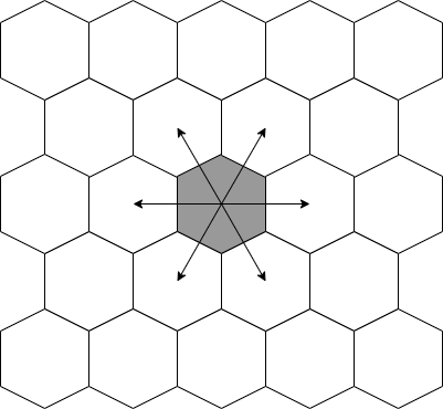
(c)

Figure 1: Illustration of the two types of partitions of the forest area implemented in FORFIS and neighbouring sub-areas of a sub-area. (a) Hexagonal partition of the forest area, (b) rectangular partition; The set $B{}$ of unit vectors pointing to neighbouring sub-areas of the gray-coloured one are indicated. (c) Same as (b) but for the hexagonal decomposition.

An element of the partition is called sub-area. The particular form of the partition, and in particular the number of partition elements $N$, is a design parameter. Intuitively, one may think of a sub-area as the area occupied by a single tree of the forest. The FORFIS software includes two different types of partitions, namely a rectangular and a hexagonal partition, cf. Fig. 1. The integer $N$ is a user input. Each sub-area has a set of neighbouring sub-areas, which can be identified by a set of unit vectors denoted by $B$. This set defines the direction of all neighbouring sub-areas to the fixed sub-area. For a rectangular partition, $B$ equals $\{e_{1},\ldots,e_{8}\}$ with $e_{1},\ldots,e_{8}\in\mathbb{R}^{2}$ as indicated in Fig. 1(b). In the hexagonal case, $B=\{e_{1},\ldots,e_{6}\}$ as indicated in Fig. 1(c). Each of the $N$ sub-areas possesses a discrete state and firefighting agents can influence this state. To be more precise, we define

$$X=\{\texttt{healthy},\texttt{afire},\texttt{burnt},\texttt{ext},\texttt{nonflam}\}^{N},$$ (3)

for the transition system (1) modelling the forest fire, where $N$ is as above. These five discrete elements characterize a healthy, burning or burnt sub-area, or a sub-area that has been extinguished. The element nonflam describes a sub-area that cannot burn. The control input is the set

$$U=\{\texttt{nop},\texttt{retardant}\}^{N},$$ (4)

which describes that either the sub-area stays untouched (element nop - no operation) or retardant has been applied (element retardant). The state of the forest fire, which is an element of $X$ in (3), changes in discrete time according to the difference inclusion (2), where the transition function $F$ will be defined subsequently.

	healthy	afire	burnt	nonflam	ext
healthy	$1-p_{\texttt{ha}}(i)$	$p_{\texttt{ha}}(i)$	$0$	$0$	$0$
afire	$0$	$1-p_{\texttt{ab}}-p_{\texttt{ae}}(v)$	$p_{\texttt{ab}}$	$0$	$p_{\texttt{ae}}(v)$
burnt	$0$	$0$	$1$	$0$	$0$
nonflam	$0$	$0$	$0$	$1$	$0$
ext	$0$	$0$	$0$	$0$	$1$

Table I: Transition probabilities for the state of the $i$th sub-area at time $t$, where $v\in\{\texttt{nop},\texttt{retardant}\}$ and $p_{\texttt{ha}}(i)$, $p_{\texttt{ab}}$, $p_{\texttt{ae}}(v)$ are as in (7)–(9).

Firstly, we assume constant wind in the area specified by a vector $w\in\mathbb{R}^{2}$, which is either $0$ (“no wind”) or of length $1$ pointing to the direction of the wind. Secondly, the subset $B(i)_{\texttt{afire}}\subseteq B$ is defined to contain those vectors that point to a neighbouring sub-area of the $i$th sub-area that is in the states afire, $i\in N$. Thirdly, we define design parameters

$$\alpha_{0}\in\left[0,1\right[,\alpha_{\textrm{wind}}\in\left]0,1\right[,\ \beta\in\left[0,1\right],\ \zeta\in\left[0,1\right],$$ (5)

where $\alpha_{0}\leq\alpha_{\mathrm{wind}}$. Intuitively, $\alpha_{0}$ determines the likelihood that a healthy area remains healthy in the case of no wind. The corresponding maximum likelihood in case of wind is determined by $\alpha_{\textrm{wind}}$. The parameter $\beta$ controls the likelihood that an area on fire becomes completely burnt. The efficiency of retardant application is determined by $\zeta$.

The transition probabilities are given by the following definitions in combination with Tab. I. The non-ignition likelihood depends on the wind $w$ and the burning neighbouring area $e\in B$ [17]:

$$\alpha(e,w)=\begin{cases}\alpha_{0},&\text{if }w=0\\ \frac{\alpha_{0}\cdot\|w\|}{1-(1-\alpha_{0}/\alpha_{\mathrm{wind}})\cdot e^{\top}w},&\text{otherwise}\end{cases},$$ (6)

$$p_{\texttt{ha}}(i) :=p_{\texttt{healthy},\texttt{afire}}(i) =1-\prod_{e\in B(i)_{\texttt{afire}}}\alpha(e,w),$$ (7)

$$p_{\texttt{ab}} :=p_{\texttt{afire},\texttt{burnt}} =\beta,$$ (8)

$$p_{\texttt{ae}}(v) :=p_{\texttt{afire},\texttt{ext}}(v) =\begin{cases}\zeta,&\text{if }v=\texttt{retardant}.\\ 0&\text{otherwise}\end{cases}$$ (9)

We note that (7) reduces to $1-\alpha_{0}^{f}$, where $f=|B(i)_{\texttt{afire}}|$, in the case $w=0$. This expression is used in [15]. To conclude, a forest fire model is specified by the $6$-tuple

$$(N,B,\alpha_{0},\alpha_{\mathrm{wind}},\beta,\zeta).$$ (10)

In Fig. 2 some graphical outputs of the FORFIS software are depicted.

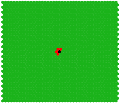
(a)

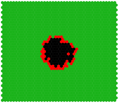
(b)

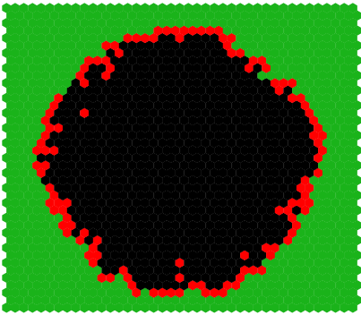
(c)

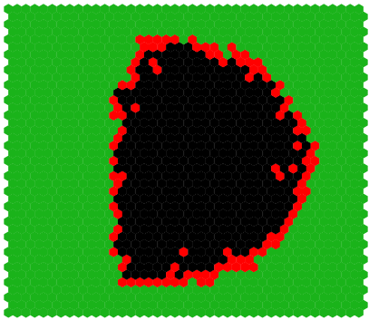
(d)

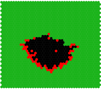
(e)

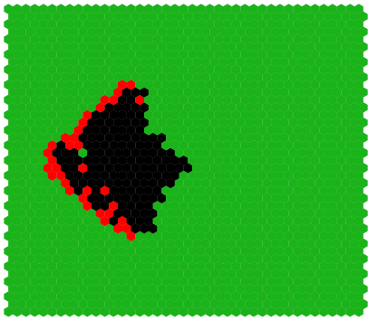
(f)

Figure 2: Graphical simulation output by FORFIS for a hexagonal decomposition of the fire area by $42\times 42$ hexagons and parameters $\alpha_{0}=0.7$, $\alpha_{\text{wind}}=1$, $\beta=0.6$ for $16$ time steps. (a) – (c) Fire spread without wind. (d) – (f) Influence of wind from the west (d), from north (e), from the east side (f) on the forest fire spread.

Implementation details

The forest fire model is implemented in the Forest class. Model configurations are made by adapting the parameters inside the configuration file as described later in Section III. The initial state $x(0)\in X$ of the fire (“fire source”) is initialized in the Forest.init_centre() method and can be freely modified there.

The data structure for the fire model is based on a two-dimensional numpy array, where each cell state corresponds to an specific integer variable.

II-C Firefighting agents model

The firefighting agents are also modelled by means of a special transition system. Specifically, the agents are modelled by the transition system $(U\times Z,X,A)$, where $U$ is as in (4),

$$Z=\{\texttt{agent},\texttt{noagent}\}^{N}$$

and therefore $A\colon(U\times Z)\times X\rightrightarrows U\times Z$. The state space of the agents transition system indicates for each of the $N$ sub-areas whether retardant has been applied (cf. (4)) and whether an agent is inside the sub-area (element agent) or not (element noagent). Consequently, the transition function $A$ models the physical movement of the agents as well as the firefighting strategy.

Figure 3: Forest fire firefighting model.

The agents transition system is interconnected with the forest fire model as depicted in Fig. 3. Intuitively, the agents transition system takes the state of the forest fire as its input and returns to the wildfire transition system an element in (4). In the current version of FORFIS, the agents are subject to certain restrictions as detailed below.

Agent’s movement

The firefighting agents can move over the whole area, where their position belongs exactly to one sub-area and two agents must not occupy the same sub-area. The agent’s movement is limited at every time step to the neighbouring cells as shown in Fig. 1 and an agent must move.

Agent’s sensors

Each agent is modelled as to be equipped with two sensors, where in the present version of the software we precisely follow [15]:

• Radio Receiver: All agents know the initial state of the forest fire. In fact, $x(0)$ is fully available for processing. Also, the state signal of the agents transition system $(u(t),z(t))\in U\times Z$ is fully available at any time $t$.

• Infrared Camera: A camera facing downwards determines the states of the sub-areas located under the agent, resulting in an image of size $3\times 3$, with the center at the agent’s position. At the edges of the grid the image is padded with artificial states nonflam. Hence, $x(t)$ is assumed not to be fully available for $t\geq 1$ but only a few components.

Moreover, every agent occupies a memory, which is a binary value initially set to false, that tracks, whether a sub-area in the state afire or burnt was sensed yet.

In the current version of FORFIS, a heuristic firefighting strategy following [15] is implemented. The firefighting process is divided into two phases. In the first phase, all agents move on a direct path towards the initial fire source in order to arrive at the fire as quickly as possible. The second phase is initiated when the agent’s memory is set to true. In this phase, the agents move counterclockwise along the fire front. Whenever an agent perceives a tree in state afire below it, retardant is applied. A formal definition of the transition function $A$ is omitted in this note due to its complexity. The influence of firefighting agents following this heuristic is illustrated in Fig. 4.

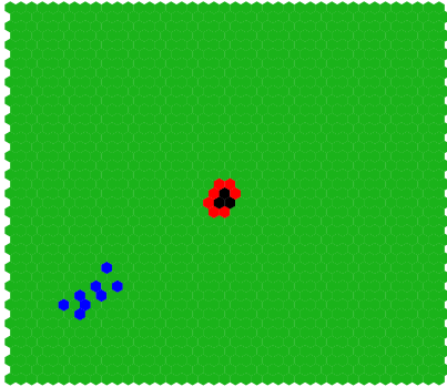
(a)

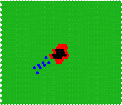
(b)

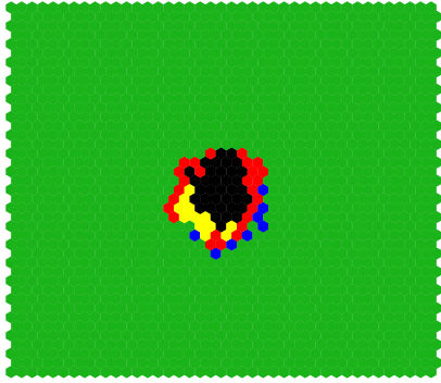
(c)

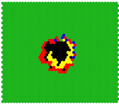
(d)

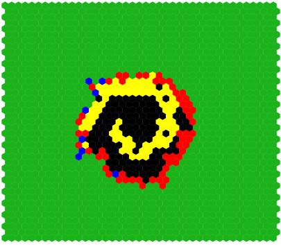
(e)

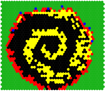
(f)

Figure 4: Graphical simulation output of FORFIS for $6$ selected time steps with $8$ firefighting agents following the heuristic strategy in [15]. The parameters are $42\times 42$ hexagons for the partition, $\alpha_{0}=0.5$, $\beta=0.6$, $\zeta=1$.

Implementation details

The agents act with a sequence of three methods, which are called within the agent.act() method as part of the agent class (refer to Fig. 5). In move(), the position of each agent is updated according to the strategy. Sense() returns the sensor data and apply_actions() applies the control actions according to the strategy. The transitions are divided into two parts. After every call of agent.act() the control actions are considered for a transition step. After six steps the whole forest updates without the agent impact.

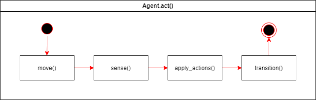
Figure 5: Sequence of the agent actions in the method agent.act()

For the sake of including new firefighting strategy algorithms there is a transparent and easy interface included in FORFIS. As part of the agent class, the method act() applies the actions as described in Section II-C.

The strategy consists of two parts: Trajectory and control actions. The trajectory is executed in the move() method and the control actions in the apply_actions() method. The algorithm to calculate the strategy can be chosen freely in those methods as long as the following interfaces are retained:

• move() gets the unique identifier and the position of an agent as the input and returns the new position.

• sense() sets the sensors and the memory with the described properties from Section II-C.

• apply_actions() takes the unique identifier of the agent and its position as the input and returns the boolean control action value with $0$ for nop and $1$ for retardant.

For the user to implement its own algorithm, set the parameter strategy in the config.yaml file to user and use the template methods in the separated file named user_strategy.py.

II-D Firefighting cost function

To evaluate the success of the firefighting strategy the user can define a metric by adapting the method success_metric() as part of the Forest class. The method calls calc_statistic(), which returns the number of sub-areas in the states healthy, afire, burnt and ext. The success_metric() method shall return the calculated cost defined by this metric.

The default cost function is

$$G(x(t),t)=c_{\texttt{healthy}}\cdot N_{\texttt{healthy}}(x(t))+c_{\texttt{ext}}\cdot N_{\texttt{ext}}(x(t))+c_{\textrm{time}}\cdot t,$$ (11)

where $N_{q}(p)=|\{i\in\{1,\ldots,N\}\mid p_{i}=q\}|$, i.e. $N_{q}(p)$ is the number of sub-areas being in the state $q$. The coefficients $c_{\texttt{healthy}}$, $c_{\texttt{ext}}$ and $c_{\textrm{time}}$ are specified in the config.yaml file.

III Graphical user interface and configuration file

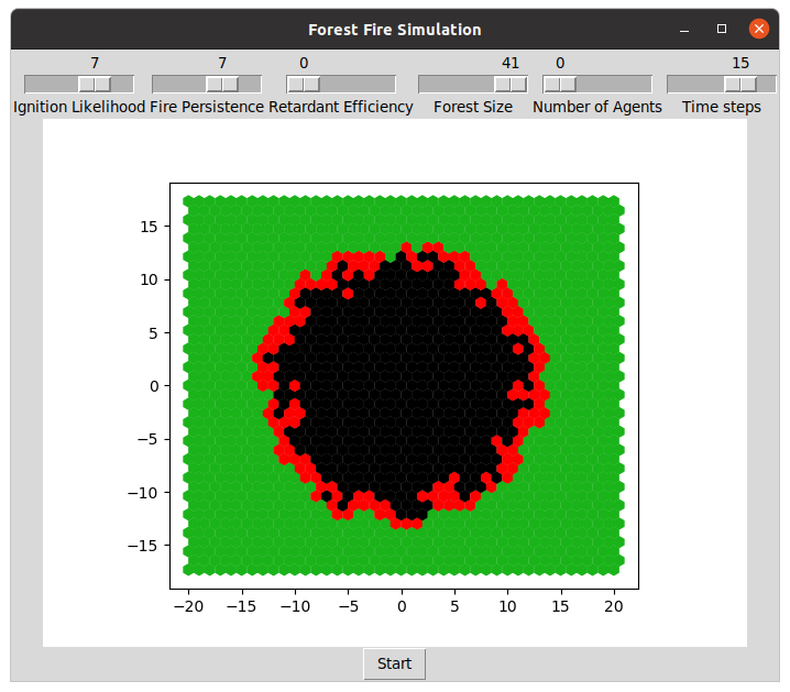
Figure 6: Graphical user interface of FORFIS

The graphical user interface (see Fig. 6) provides a button to start a new simulation, a visualization area and the following basic model-specific and general modification parameters:

• Ignition Likelihood $l$: $l\in[0,10]$ such that $\alpha=1-\frac{l}{10}$

• Fire Persistence $p$: $p\in[0,10]$ such that $\beta=\frac{p}{10}$

• Retardant Efficiency $e$: $e\in[0,10]$ such that $\zeta=\frac{e}{10}$

• Forest Size $n$: Creates a grid of $n\times n$ cells

• Number of Agents $a$: Includes $a$ agents. $0$ for a forest fire simulation without firefighting agents.

• Time Steps $\tau$: Simulation will last $\tau$ time steps. Choose $0$ for a full simulation until the fire is extinguished or fully burnt.

The described configurations as well as the following additional options can also be predefined in a configuration file called config.yaml:

• GUI: Boolean value to run the simulation with or without the graphical user interface

• agent_mode: Strategy algorithm, $Haksar$ for heuristic inspired by [15] or $user$ for user-defined algorithm. See Section II-C.

• logfile: Boolean value to save the simulation results in a log file named with the start date and time of the simulation.

• grid: rectangular for a rectangular cell geometry, hexagonal for a hexagonal cell geometry.

References

- [1] J. M. Diaz, “Economic impacts of wildfire,” Southern Fire Exchange, vol. 498, pp. 2012–7, 2012.
- [2] H. Pozniak, “Are wildfires getting worse?” Engineering & Technology, vol. 14, no. 1, pp. 68–72, 2019.
- [3] R. C. Rothermel, A mathematical model for predicting fire spread in wildland fuels. Intermountain Forest & Range Experiment Station, Forest Service, US …, 1972, vol. 115.
- [4] G. Albinet, G. Searby, and D. Stauffer, “Fire propagation in a 2-D random medium,” Journal de Physique, vol. 47, no. 1, pp. 1–7, 1986. [Online]. Available: https://hal.archives-ouvertes.fr/jpa-00210180
- [5] K. C. Clarke, J. A. Brass, and P. J. Riggan, “A cellular automaton model of wildfire propagation and extinction,” Photogrammetric Engineering and Remote Sensing, vol. 60, no. 11, pp. 1355–1367, 1994.
- [6] A. Hernández Encinas, L. Hernández Encinas, S. Hoya White, A. Martín del Rey, and G. Rodríguez Sánchez, “Simulation of forest fire fronts using cellular automata,” Advances in Engineering Software, vol. 38, no. 6, pp. 372–378, 2007, advances in Numerical Methods for Environmental Engineering.
- [7] L. Hernández Encinas, S. Hoya White, A. Martín del Rey, and G. Rodríguez Sánchez, “Modelling forest fire spread using hexagonal cellular automata,” Applied Mathematical Modelling, vol. 31, no. 6, pp. 1213–1227, 2007.
- [8] A. Alexandridis, D. Vakalis, C. Siettos, and G. Bafas, “A cellular automata model for forest fire spread prediction: The case of the wildfire that swept through spetses island in 1990,” Applied Mathematics and Computation, vol. 204, no. 1, pp. 191 – 201, 2008.
- [9] A. L. Sullivan, “A review of wildland fire spread modelling, 1990-present 3: Mathematical analogues and simulation models,” International Journal of Wildland Fire, 2007.
- [10] G. D. Papadopoulos and F.-N. Pavlidou, “Software tools for wildfire monitoring,” in Proc. 5th Intl. Conf. Interdiciplinarity in Education (ICIE) June. Citeseer, 2010.
- [11] K. Tolhurst, B. Shields, and D. Chong, “Phoenix: development and application of a bushfire risk management tool.” Australian journal of emergency management, vol. 23, no. 4, pp. 47–54, 2008.
- [12] M. A. Finney, “FARSITE: a fire area simulator for fire managers,” in In: Weise, David R.; Martin, Robert E., technical coordinators. The Biswell symposium: fire issues and solutions in urban interface and wildland ecosystems; February 15-17, 1994; Walnut Creek, California. Gen. Tech. Rep. PSW-GTR-158. Albany, CA: Pacific Southwest Research Station, Forest Service, US Department of Agriculture; p. 55-56, vol. 158, 1995.
- [13] C. Miller, J. Hilton, A. Sullivan, and M. Prakash, “SPARK – a bushfire spread prediction tool,” in Environmental Software Systems. Infrastructures, Services and Applications, R. Denzer, R. M. Argent, G. Schimak, and J. Hřebíček, Eds. Cham: Springer International Publishing, 2015, pp. 262–271.
- [14] A. Somanath, S. Karaman, and K. Youcef-Toumi, “Controlling stochastic growth processes on lattices: Wildfire management with robotic fire extinguishers,” in 53rd IEEE Conf. on Decision and Control, 2014, pp. 1432–1437.
- [15] R. N. Haksar and M. Schwager, “Distributed deep reinforcement learning for fighting forest fires with a network of aerial robots,” in 2018 IEEE/RSJ Intl. Conf. Intelligent Robots and Systems (IROS), 2018, pp. 1067–1074.
- [16] M. Montenegro, R. López, R. Menchaca-Méndez, E. Becerra, and R. Menchaca-Méndez, “A parallel rollout algorithm for wildfire suppression,” in Telematics and Computing, M. F. Mata-Rivera, R. Zagal-Flores, and C. Barria-Huidobro, Eds. Cham: Springer International Publishing, 2020, pp. 244–255.
- [17] P. Johnston, J. Kelso, and G. J. Milne, “Efficient simulation of wildfire spread on an irregular grid,” International Journal of Wildland Fire, vol. 17, no. 5, pp. 614–627, 2008.