A sheet-like structure in the proximity of compact DNA

Abstract

We determine the phase diagram of DNA with inter- and intra-strand native-pair interactions that mimic the compaction of DNA. We show that DNA takes an overall sheet-like structure in the region where an incipient transition to a compact phase would have occurred. The stability of this phase is due to the extra entropy from the folding of the sheet, which is absent in the remaining polymer-like states of the phase diagram.

I Introduction

A common bacterium like a rod-shaped E.coli of size $2\mu$m$\times 1\mu$m$\times 1\mu$m stores a $1.5$mm long DNA of $N=4\times 10^{6}$ base pairs. Even if the DNA takes an entropy-driven random coil form its size $\sim\sqrt{N}\sim 5\mu$m would still be too large to fit in the cell . The evolutionary strategy of encapsulating protein-compactified chromosomes in a nucleus encased by membranes, as in eukaryotes, does not apply to prokaryotes that lack a nucleus, but still, compaction would resolve the DNA-packing puzzle. Over the years, with support from the dynamic light scattering [2] and the high-resolution single-molecule imaging [3] studies, the proposal of a boundaryless region called nucleoid [4, 5] is gaining ground, which creates an environment for DNA to collapse into a compact form.

DNA in a salt solution behaves as a polymer in a good solvent, called the swollen or coil phase, where excluded volume interactions dominate the overall behaviour [7, 8]. A surprising result was that a long DNA, much larger than its persistence length, can be collapsed into a compact shape [9] by adding ethanol, different types of cations, hydrophilic polymers, or organic solvents [10, 11, 12]. The collapse of DNA remained elusive in earlier studies because of the requirement of large lengths, though the tendency of liquid-crystalline ordering [13] was recorded for oligonuceotides. This tendency of local arrangement persists in the collapsed phase [9], suggesting the condensed DNA phase [6] to be different from the globular (collapsed) phase of a polymer below the theta point [7]. Moreover, as all base pairs should be easily accessible, an ordered or correlated structure would have a functional advantage. Consequently, a fractal globule phase has been proposed as a possible phase, where DNA is compact but without any knots [14]—a phase different from the usual compact globule. Such a fractal phase with power-law correlations of monomers finds support in the human genome [15].

As a tertiary structure of DNA, the compact phase is found to be insensitive to the secondary structure like B, A, or Z [16]. DNA also undergoes a temperature (or pH) induced melting transition and a force-induced unzipping transition, both involving cooperative breakings of the hydrogen bonds of the base pairs [17]. In a bacterial environment, melting or unzipping is required for replication and, at least locally, for transcription to make the bases accessible. With the DNA in the nucleoid, a question arises: does a compact DNA melt? Thus the phenomenon of DNA compaction in nucleoids is a topic of interest in biology, polymer physics, and also for practical applications because of the ease of insertion of a compact DNA in bio-systems, e.g., in gene therapy [18].

The compaction phenomenon has been studied in some detail by treating DNA as polymers or polyelectrolytes. For example, a recent study focussed on the melting temperature variations in the presence of attraction exclusively between bound pairs [19]. Other proposals include compaction induced by phase separation, mechanisms based on neutralizing charges on DNA, or the presence of small cations in solutions [4]. In sec II, we introduce the model and the details of the simulation. The various phases and the phase diagram are determined in sec III where a heuristic argument is also presented to motivate the phases. The summary of the findings is in sec IV. Some of the details are given in the supplementary material in the form of figures.

II Model and Method

We explore how compaction modifies double-stranded DNA (dsDNA) melting. The interactions are chosen to favour a folded conformation of dsDNA, thereby avoiding a generic globular phase in a poor solvent. Our coarse-grained model consists of two single-stranded DNA (ssDNA), A and B (also called polymers), with native DNA base pairing and an additional intra-strand base-pairing type interaction that allows each polymer to fold on itself. The model potential considered for polymer A or B is

$$\left.\begin{array}[]{ll}E_{A}/k_{B}T\\ E_{B}/k_{B}T\end{array}\right\} = \sum_{i=1}^{N-1}K(d_{i,i+1}-d_{0})^{2}+4\sum_{\rm N-nat}\bigg{(}\frac{\sigma_{i,j}}{d_{i,j}}\bigg{)}^{12}$$ (4)

$$+4{\epsilon_{s}}\sum_{\rm N.C.}\bigg{[}\bigg{(}\frac{\sigma_{i,j}}{d_{i,j}}\bigg{)}^{12}-\bigg{(}\frac{\sigma_{i,j}}{d_{i,j}}\bigg{)}^{6}\bigg{]},$$

where N.C. and N-nat denote native and non-native contacts. Here, each polymer consists of $N(=36)$ beads, the distance between beads $d_{i,j}$ is defined as $|\bm{r}_{i}-\bm{r}_{j}|$, where $\bm{r}_{i}$ and $\bm{r}_{j}$ are the position vectors of beads $i$ and $j$, respectively with $i,j\in[1,N]$. We use dimensionless distances with $\sigma_{i,j}=1$ and $d_{0}=1.12$. The energy parameters in the Hamiltonian are in units of $k_{B}T$ where $k_{B}$ is the Boltzmann constant and $T$ is the temperature. The harmonic (first) term on the rhs with dimensionless spring constant $K(=100)$ couples the adjacent beads along the chain [20, 21]. The second term is a repulsive potential that prevents overlap of non-native pairs of monomers of chain A (and B) [21, 22, 23]. The third term is the van der Waals energy (involving $\epsilon_{s}$) that allows pairing of non bonded monomers at position $i$ and $N-i+1$(Fig. 1a). These intra-strand pairings are the native contacts (N.C.) in Eq. (4). The inter-strand interactions are given by

$$\frac{E_{A,B}}{k_{B}T} = \sum_{\rm N.C.}4{\epsilon_{p}}\bigg{[}\bigg{(}\frac{\sigma_{i,j}}{d_{i,j}}\bigg{)}^{12}-\bigg{(}\frac{\sigma_{i,j}}{d_{i,j}}\bigg{)}^{6}\bigg{]}$$ (5)

$$+\sum_{\rm N-nat}4\bigg{(}\frac{\sigma_{i,j}}{d_{i,j}}\bigg{)}^{12}.$$

The base pairing between chains A and B is considered using the first term on the rhs of Eq. 5. The native base-pair contacts (same $i$ of both the chains, see Fig. 1b) are such that it results in a ladder structure of dsDNA [20, 21]. The second repulsive term of the potential energy in Eq. (5) prevents non-native pairings of monomers of chains A and B [20, 21, 22, 23]. We obtain the dynamics of system by solving the set of Brownian equations [28]

$$\frac{d\bm{r_{i}}}{dt}=\frac{1}{\zeta}(\bm{F}_{c}+\bm{\Gamma}).$$ (6)

Here, $\bm{F}_{c}=-\bm{\nabla}E$ is the conservative force and $E$ is the sum of $E_{A}$, $E_{B}$ and $E_{A,B}$. $\zeta$ is the friction coefficient, and $\bm{\Gamma}$ is the random force, a white noise with zero mean and correlation $\langle\Gamma_{i}(t)\Gamma_{j}(t^{\prime})\rangle=2\zeta k_{B}T\delta_{i,j}\delta(t-t^{\prime})$. The temperature of the simulation is set to be constant $T=0.16$. The equation of motion is integrated using a Euler method. We obtained the phase diagram from our simulation by monitoring the peak position in energy fluctuation as a function of intra-strand energy ($\epsilon_{s}$) at a fixed base-pairing energy ($\epsilon_{p}$) and vice versa.

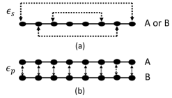
Figure 1: Schematic diagram for the native contacts: (a) intra-strand contacts (dotted lines)in each polymer chain (A or B) with energy $\epsilon_{s}$ and (b) base-pair contacts (dotted lines) between chains A and B with energy $\epsilon_{p}$.

III Results

A Phase diagram in $\epsilon_{s}-\epsilon_{p}$ plane

To understand the phase behaviour, let us consider a simpler model with energy based on contact numbers. The interaction energy can be written as

$$\frac{E}{k_{B}T}=-\epsilon_{p}n_{\rm{AB}}-\epsilon_{s}(n_{\rm{AA}}+n_{\rm{BB}}),$$ (7)

where $n_{\rm{AB}}$ is the number of native base pairs between the two chains, with $-\epsilon_{p}$ as the energy for each pair, $n_{\rm{AA}}$, $n_{\rm{BB}}$ are the number of intra-strand pairs with $-\epsilon_{s}$ as the energy per intra-strand pair. For a given DNA, $\epsilon_{s}$, $\epsilon_{p}$ change with temperature with $\epsilon_{s}/\epsilon_{p}=$ constant.

In the $\epsilon_{s}$-$\epsilon_{p}$ plane, there are four fixed points (FP) or limiting points which are representatives of the four phases one would expect naively, viz,

• State-I: a denatured phase of two free ssDNA chains (FP: $\epsilon_{s}=\epsilon_{p}=0$)

• State-II: bound A-B as dsDNA in a swollen phase (FP: $\epsilon_{s}=0,\epsilon_{p}=\infty$)

• State-III: two folded ssDNA in the denatured phase (FP: $\epsilon_{s}=\infty,\epsilon_{p}=0$)

• State-IV: dsDNA in the folded state (FP: $\epsilon_{s}=\epsilon_{p}=\infty$)

Assuming an all-or-none state, i.e., either all pairs are formed or all broken, the free energy of phase I is $F_{I}/k_{B}T=-S_{I},$ while for phase II, it is $F_{II}/k_{B}T=-N\epsilon_{p}-S_{II},$ where $S_{I}$ and $S_{II}$ are the total entropies of the chains in the respective phases. A first-order transition then takes place at $\epsilon_{p}=(S_{I}-S_{II})/N$, and the phase boundary is expected to be vertical in the $\epsilon_{s}$-$\epsilon_{p}$ plane. By symmetry, the transition from I to III should also be at the same value of $\epsilon_{s}$, and the boundary is horizontal, independent of $\epsilon_{p}$. Similar vertical or horizontal boundaries are expected for the III$\leftrightarrow$IV and the II$\leftrightarrow$IV transitions. Deviations from linearity might occur near the intersection of the four transition lines because of the proximity of other phases. Can there be other intermediate phases in this two-parameter phase diagram?

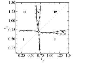
Figure 2: The phase-diagram shows the occurrence of various states in different regions of the $\epsilon_{s}$-$\epsilon_{p}$ plane. These states are State-I (two free ssDNA), State-II(dsDNA), State-III (2 folded ssDNA), State-IV (folded dsDNA), and State-V (sheet). The dashed line corresponds to $\epsilon_{s}=\epsilon_{p}$ and goes through the intersection point of the phase boundaries.

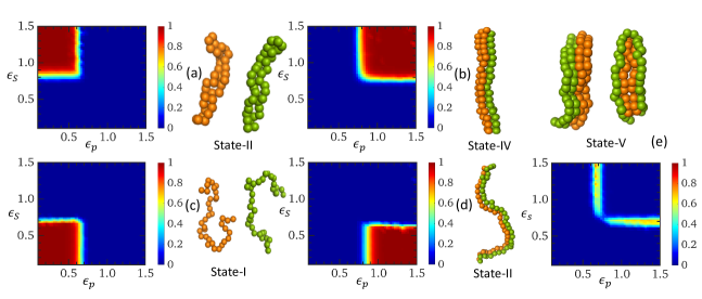
Figure 3: The probability of occurrence of different states in the phase diagram. (a-d) the right panel shows four different states of polymer A (green) and polymer B (orange); State-I (two free ssDNA), State-II (one dsDNA), State-III (two folded ssDNA), and State-IV (folded dsDNA). In the left panel, color map shows the probability of occurrence of a state (next to it) in different regions of the $\epsilon_{s}$-$\epsilon_{p}$ plane. (e) A sheet structure formed from polymer A (green) and polymer B (orange) (top panel) and their occurrence probability in different regions of the $\epsilon_{s}$-$\epsilon_{p}$ plane (bottom panel). The sheet structure occurs in the Y-regions of the phase diagram.

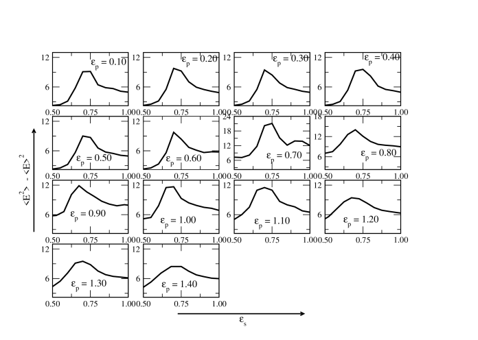
Figure S1: Energy fluctuations as a function of $\epsilon_{s}$ at different values of $\epsilon_{p}$.

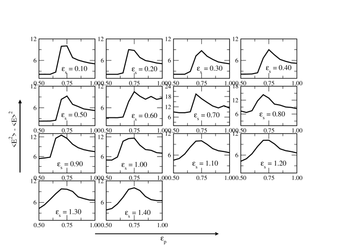
Figure S2: Energy fluctuations as a function of $\epsilon_{p}$ at different values of $\epsilon_{s}$.

To address the above question, The phase boundary is plotted in Fig. 2. We obtain a horizontal phase boundary close to $\epsilon_{s}=0.75$ for $\epsilon_{p}<1.00$, which starts bifurcating into two branches for $\epsilon_{p}>1.00$ (wider peak in energy fluctuations, Fig. S1 [24]). Similarly, we observe a vertical phase boundary close to $\epsilon_{p}=0.75$ for $\epsilon_{s}<0.80$, which starts bifurcating into two branches for $\epsilon_{s}>0.80$ (Fig. S2 ). Overall, the phase diagram is symmetric, except for the point at which the bifurcation starts appearing in the phase diagram ($\epsilon_{p}>1.00$, and $\epsilon_{s}>0.80$). In addition to the horizontal and vertical boundaries, as suggested by the energy construct, we obtain two additional regions (Y-regions) in the phase diagram (Fig. 2). The average over two boundaries of each Y-region further corroborates the horizontal or vertical nature of the boundaries in the phase diagram.

B Probability of occurrence of different phases

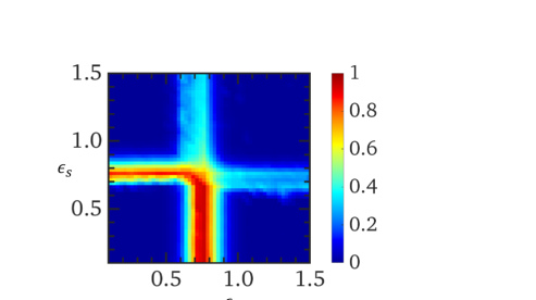
Figure S3: The probability of occurrence of state-VI (mixed states).

To get the microscopic view of the phase diagram, we probe the probability of occurrence of different structures in different regions of the phase diagram. The structures can be quantified by the number of base pairs ($n_{p}$) and the number of intra-strand pairs ($n_{s}$) present in a given conformation as below (the maximum number of allowed pairs is $n_{max}=N$)
State-I: $n_{p}$ and $n_{s}$ both are small ($<0.3n_{max}$),
State-II: large $n_{p}(>0.8n_{max}$) and small $n_{s}(<0.3n_{max})$,
State-III: small $n_{p}(<0.3n_{max})$ and large $n_{s}(>0.8n_{max})$,
State-IV: $n_{p}$ and $n_{s}$ both are large ($>0.8n_{max}$).
The probability of occurrence of different states defined above ($P_{I}$, $P_{II}$, $P_{III}$ and $P_{IV}$) are plotted in Fig. 3. We see from Fig. 3c, that $P_{I}=1$ for lower values of $\epsilon_{p}$ and $\epsilon_{s}$ and decreases as we increase $\epsilon_{p}$ or $\epsilon_{s}$. For very large values of $\epsilon_{p}$ or $\epsilon_{s}$, $P_{I}$ becomes zero, and state II or state III starts appearing with small probabilities (Figs. 3d, 3a). For larger values of $\epsilon_{p}$ and lower values of $\epsilon_{s}$ (the lower branch of the horizontal Y-region), $P_{II}=1$ (Fig. 3d) while for larger values $\epsilon_{s}$ and lower values of $\epsilon_{p}$ (the left branch of the vertical Y-region), $P_{III}=1$ (Fig. 3a), respectively. These states persist as we increase $\epsilon_{p}$ or $\epsilon_{s}$. State IV starts appearing on the right of the vertical Y branch and above the horizontal Y branch, $P_{IV}=1$ (Fig. 3b) at larger values of $\epsilon_{p}$ and $\epsilon_{s}$, with $P_{IV}=0$ elsewhere. Many mixed states (State-VI) appear with finite probability ($P_{VI}$) near the phase boundaries (coexistence line) (Fig. S3-S4). The observation of states (I-IV) are in accordance with those predicted by the simple model of energy considered earlier. However, the simple model needs modifications to provide insight about the Y-regions and the corresponding phases in the phase diagram.

It should be emphasized here that the vertical (horizontal) Y-region starts appearing around intermediate values of $\epsilon_{p}(\epsilon_{s})$, where a large energy $\epsilon_{s}(\epsilon_{p})$ is already present in the system. A comparable energy scale may stabilize an intermediate phase between State III (State II) and State IV. As we cross the vertical Y-region, $n_{s}$ ($>0.8n_{max}$) is almost unchanged (for large $\epsilon_{s}$) and $n_{p}$ goes from zero ($<0.3n_{max}$ for small $\epsilon_{p}$) to maximum ($>0.8n_{max}$ for large $\epsilon_{p}$). In the phase diagram, one may look further for a state with intermediate $n_{p}$ and its occurrence probability. Motivated by this, we define a State-V ($n_{s}>0.8n_{max}$ and $0.35n_{max}<n_{p}<0.6n_{max}$). This state has a very high occurrence probability ($P_{V}\sim 0.6$) as can be seen in Fig. 3e color map, and it appears exactly in the vertical Y-region of the phase diagram though absent elsewhere. This State-V is a sheet-like structure (Fig. 3e, upper left structure), formed as two folded ssDNA come close to each other. A similar sheet-like structure ($n_{p}>0.8n_{max}$ and $0.35n_{max}<n_{s}<0.6n_{max}$, Fig. 3e, upper right structure) occurs with high probability in the horizontal Y-region, with the only difference that $n_{s}$ and $n_{p}$ flip their positions. Moreover, two folded ssDNA (state III, for large $\epsilon_{s}$) can be close to each other to form a sheet structure, without any geometrical constraint, by introducing bonds of comparable energy $\epsilon_{p}$. However, forming the sheet from state II (large $\epsilon_{p}$) is more difficult energetically. As the backbone of dsDNA (State-II) consists of springs (first term of Eq. 4), the formation of a sheet-like structure requires the stretching of a few springs at one side of the sheet. Therefore, the backbone always puts geometrical constraints on one side of the sheet. This extra geometric constraint results in the asymmetry in the starting points of vertical and horizontal Y-regions.

The four states, State-I to State-IV, are polymer-like. If $s_{0}$ is the entropy per monomer of a swollen polymer, we shall have, for the four states I to IV,

$$S_{I}=2Ns_{0},S_{II}=Ns_{0},\ S_{III}=2\frac{N}{2}s_{0},{\rm\ and\ }S_{IV}=\frac{N}{2}s_{0}.$$

The symmetry of the phase diagram follows from the phase boundaries

$$\epsilon_{p}\big{|}_{I\rightarrow II}=s_{0},{\rm\ and\ }\epsilon_{s}\big{|}_{I\rightarrow III}=s_{0}.$$

This picture is validated by more or less vertical or horizontal phase boundaries (Fig. 2), as explained in the previous paragraph. In contrast to the four states, State-V takes a flexible sheet-like structure with an extra source of entropy from the possibility of folding the sheet. The free energy of State-V, with $S_{V}$ as its entropy, is

$$\frac{F_{V}}{k_{B}T}=-\frac{N}{2}\epsilon_{p}-N\epsilon_{s}-S_{V}.$$

Therefore, the III-V and the IV-V transitions would take place at

$$\epsilon_{p}=2(S_{III}-S_{V})/N\ {\rm(for\ III\leftrightarrow V)},$$ (8a)

$$\epsilon_{p}=2(S_{V}-S_{IV}/N){\ \rm(for\ IV\leftrightarrow V)},$$ (8b)

which require $S_{III}>S_{V}>S_{IV}$. In other words, State-V would occur in the neighbourhood of the putative III-IV transition. Similar arguments can be used for the II-IV phase boundary.

C Melting of compact DNA

The replication and transcription process of DNA requires the separation of DNA strands. It is now well established experimentally and theoretically [17, 25, 26, 27, 28, 29, 30, 31] that DNA undergoes a temperature (or pH) induced melting transition and a force-induced unzipping transition, both involving a cooperative breaking of the base pairs. To probe the melting transition of a compact DNA, we follow the evolution of different states by varying the interaction energy along the $\epsilon_{p}/\epsilon_{s}=1$ line (the dashed line in Fig. 2). From our simulations, we compute the occurrence probabilities of different states (Fig. 4). We start with $\epsilon_{s}=\epsilon_{p}=1.50$, where only state-IV (folded dsDNA) appears with $P_{IV}=1$ until we are close to the intersection point in the phase diagram. Here, $P_{IV}$ decreases, and many mixed configurations appear which we call state-VI (see Fig. S4, supplementary material). As the intersection point is a coexistence point of at least four phases, many mixed configurations are expected to occur. In fact, we find $P_{VI}\sim 1$ and $P_{V}\sim 0.10$. The scenario changes as we go just below the intersection point of the phase diagram along the chosen line (Fig. 2). $P_{I}$ starts picking up and State-I becomes the only state ($P_{I}=1$) for lower values of $\epsilon_{s}$. In short, we see the melting of a compact DNA along the chosen line. In contrast, for any other line with $\epsilon_{p}/\epsilon_{s}\neq 1$, the dsDNA to ssDNA transformation necessarily entails one other state.

IV Conclusions

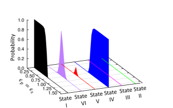
Figure 4: Probability of occurrence of different states along the line with slope one ($\epsilon_{s}/\epsilon_{p}=1$) in Fig.2 (dashed line).

In this paper, we studied the compaction of DNA by considering two types of effective interactions, (i) inter-strand native-pair interactions that favour dsDNA formation, and (ii) intra-strand native-pair interactions that promote the folding of each strand of DNA. The varying strengths of these effective interactions mimic the role of different cellular environments that lead to the compaction of DNA inside the cell. We observed five different phases in the phase diagram as summarized in Fig. 2. There are transitions taking two free ssDNA (State-I), at lower values of interaction energies, to either a bound dsDNA (State-II) or two folded ssDNA (State-III), as one of the interaction energies (intra-strand or inter-strand) is increased, keeping the other one at a lower value. For larger values of both interaction energies, dsDNA folds onto itself (State-IV), a state reminiscent of a compact DNA. If a heating process takes a compact DNA to ssDNA along a line through the intersection point, there will be a genuine melting point. Otherwise another phase will always intervene. Furthermore, we observe from our simulations a sheet-like arrangement (State-V); it occurs around the region where the III-IV or the II-IV transitions would have occurred and is unlike any of the other four states (I to IV), which are polymer-like. The stability of the phase comes from the extra folding entropy acquired by a sheet-like structure.

Acknowldgments

GM gratefully acknowledges the financial support from SERB India for a start-up grant with file Number SRG/2022/001771 and acknowledges the HPC computing facility at Ashoka University.

Supplementary Material

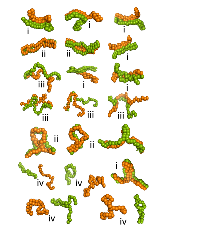
Figure S4: Some representative conformations in state-VI, e.g. A sheet open at one or both the ends(i), folded dsDNA with loop or y-fork(ii), A dsDNA with loop or y-fork (iii), folded ssDNA with loop or yfork (iv). These are all examples of two phases coexisting along the length of DNA.

References

- Note [1] The persistence length of DNA is nm or bp. The radius of gyration for a random walk of units each of length is m. One may take the Kuhn units of length , but that does not affect the order of magnitude estimate. If the excluded volume interactions are taken into account the size of the swollen conformation would be much larger. If excursions beyond the average size is taken into account, the actual size would be larger than the estimate above.
- Dias et al. [2005] R. S. Dias, J. Innerlohinger, O. Glatter, M. G. Miguel, and B. Lindman, J. Phys. Chem. B 109, 10558 (2005).
- Stracy et al. [2014] M. Stracy, S. Uphoff, F. G. d. Leon, and A. N. Kapanidis, FEBS Lett. 588, 3585 (2014).
- Joyeux [2015] M. Joyeux, J. Phys.: Condens. Matter 27, 383001 (2015).
- Verma et al. [2019] S. C. Verma, Z. Qian, and S. L. Adhya, PLoS Genet 15, e1008456 (2019).
- [6] The words “compact DNA” and “condensed DNA” will be used interchangeably. Similarly, DNA-condensation and DNA-compaction are used synonymously.
- Bhattacharjee et al. [2013] S. M. Bhattacharjee, A. Giacometti, and A. Maritan, J. Phys.: Condens. Matter 25, 503101 (2013).
- Valle et al. [2005] F. Valle, M. Favre, P. De Los Rios, A. Rosa, and G. Dietler, Phys. Rev. Lett. 95, 158105 (2005).
- Bloomfield [1996] V. A. Bloomfield, Curr Opin Struct Bio 6, 334 (1996).
- Teif and Bohinc [2011] V. B. Teif and K. Bohinc, Prog Biophys Mol Biol. 105, 208 (2011).
- Ke et al. [210] F. Ke, Y. K. Luu, M. Hadjiargyrou, and D. Liang, PLoS ONE 5, e13308 (210).
- Mikhailenko et al. [2000] S. V. Mikhailenko, V. G. Sergeyev, A. A. Zinchenko, M. O. Gallyamov, I. V. Yaminsky, and K. Yoshikawa, Biomacromolecules 1, 597 (2000).
- Leforestier and Livolant [1993] A. Leforestier and F. Livolant, Biophys. J. 65, 56 (1993).
- Grosberg et al. [1988] A. Y. Grosberg, S. K. Nechaev, and E. I. Shakhnovich, J. Phys. France 49, 2095 (1988).
- Lieberman-Aiden et al. [2009] E. Lieberman-Aiden et al., Science 326, 289 (2009).
- Silvia Hormeño et al. [2011] S. Silvia Hormeño, F. Moreno-Herrero, B. Ibarra, J. L. Carrascosa, J. M. Valpuesta, and J. R. Arias-Gonzalez, Biophys. J. 100, 2006 (2011).
- Bhattacharjee [2000] S. M. Bhattacharjee, J. Phys. A: Math. Gen. 33, L423 (2000), (arXiv:cond-mat/9912297).
- Hansma et al. [1998] H. G. Hansma, R. Golan, W. Hsieh, C. P. Lollo, P. Mullen-Ley, and D. Kwoh, Nucleic Acids Research 26, 2481 (1998).
- Majumdar [2023] D. Majumdar, J. Stat. Phys. 190, 14 (2023).
- Mishra et al. [2011] G. Mishra, D. Giri, M. S. Li, and K. Sanjay, J. Chem. Phys. 135, 035102 (2011).
- Kumar and Mishra [2013] S. Kumar and G. Mishra, Phys. Rev. Lett. 110, 258102 (2013).
- Allen and Tildesley [1987] M. P. Allen and D. Tildesley, Computer Simulations of Liquids (Oxford Science, Oxford, UK, 1987).
- Frenkel and Smit [1987] D. Frenkel and B. Smit, Understanding Molecular Simulation (Oxford Science, Oxford, UK, 1987).
- [24] Figs. S1-S4 refer to figures in the supplementary material at the end.
- terBurg et al. [2023] C. ter Burg, P. Rissone, M. Rico-Pasto, F. Ritort, and K. J. Wiese, Phys. Rev. Lett. 130, 208401 (2023).
- Danilowicz et al. [2004] C. Danilowicz, Y. Kafri, R. S. Conroy, V. W. Coljee, J. Weeks, and M. Prentiss, Phys. Rev. Lett. 93, 078101 (2004).
- Koch et al. [2002] S. J. Koch, A. Shundrovsky, B. C. Jantzen, and M. D. Wang, Biophys. J 83, 1098 (2002).
- Kumar and Li [2010] S. Kumar and M. S. Li, Phys. Rep. 486, 1 (2010).
- Rudnizky et al. [2018] S. Rudnizky, H. Khamis, O. Malik, A. H. Squires, A. Meller, P. Melamed, and A. Kaplan, Nucleic Acids Res. 46, 1513 (2018).
- Kapri [2012] R. Kapri, Phys. Rev. E. 86, 041906 (2012).
- Singh and Granek [2016] A. R. Singh and R. Granek, J. Chem. Phys. 145, 144101 (2016).