Stationary and moving bright solitons in Bose-Einstein condensates
with spin-orbit coupling in a Zeeman field

Abstract

With the discovery of various matter wave solitons in spin-orbit-coupled Bose-Einstein condensates (BECs), exploring their properties has become increasingly significant. We mainly study stationary and moving bright solitons in spin-orbit-coupled spin-1 BECs with or without a Zeeman field. The bright solitons correspond to the plane wave (PW) and standing wave (SW) phases. With the assistance of single-particle energy spectrum, we obtain the existence domains of PW and SW solitons by analytical and numerical methods. The results indicate that the interaction between atoms is also a key factor determining the existence of solitons. In addition, we systematically discuss the stability domains of PW and SW solitons, and investigate the impact of different parameters on the stability domains. We find that PW solitons are unstable when the linear Zeeman effect reaches a certain threshold, and the threshold is determined by other parameters. The linear Zeeman effect also leads to the alternating distribution of stable and unstable areas of SW solitons, and makes SW solitons stably exist in the area with stronger ferromagnetism. Finally, we analyze the collision dynamics of different types of stable solitons.

I Introduction

Since the spin-orbit coupling (SOC) of neutral atoms was realized for the first time in 2011 [1], Bose-Einstein condensates (BECs) with SOC have received much attention, which is a good platform for studying quantum phenomena, such as superfluidity in liquid helium [2] and superconductivity in metals [3]. The artificial SOC is highly adjustable and equivalent to an equal weight mixing of Rashba [4] and Dresselhaus [5] SOC. Naturally, it is significant for us to study condensed matter effects, such as topological insulators [6] and spin Hall effect [7].

The SOC effect makes single-particle ground state degenerate. For this reason, a spinor BEC with SOC exhibits a variety of phases and a richer ground state phase diagram [8, 9, 10, 11, 12, 13, 14]. Each phase has its own characteristics [15, 16, 17, 18]. For example, the plane wave (PW) phase features nonzero magnetizations, the standing wave phase (SW) has supersolid properties [19], and the zero momentum phase is analogous to a conventional BEC without SOC. Besides, the SOC effect leads to many intriguing dynamic phenomena [20, 21, 22, 23, 24, 25]. These are all closely related to matter wave bright solitons corresponding to these phases. When the Zeeman effect and Raman coupling are not considered, there is a large amount of research on PW and SW bright solitons in spinor BECs with SOC [26, 27, 28, 29, 30, 31, 32]. However, considering the Zeeman effect or Raman coupling, the research mainly focuses on PW bright solitons in different spinor BECs with SOC [33, 34, 35, 36], and SW bright solitons in spin-1/2 BECs with SOC [38, 37, 39, 40, 41]. SW bright solitons in spin-1 BECs with SOC have not been systematically explored in the presence of Zeeman field, which enriches the magnetic behaviors of the system [42, 43]. To our knowledge, previous studies focused on the types of bright solitons in spinor BECs with SOC, with less attention paid to the existence and stability of bright solitons. There are some systematic studies on spin-1/2 BEC systems with SOC [39, 40, 44], but not on spin-1 BEC systems with SOC. Additionally, the mean-field ground state of a spin-1 BEC with SOC and ferromagnetic (antiferromagnetic) interaction favors a PW (SW) soliton [8, 10]. It does not mean that PW (SW) solitons can not exist in antiferromagnetic (ferromagnetic) BECs with SOC, and thus analyzing the existence and stability domains of these solitons is necessary. Moreover, the SOC effect breaks the Galilean invariance. It impedes us to construct moving bright solitons whose profiles are invariable during their evolution [37, 45], especially moving SW bright solitons. Therefore, it is challenging and significant to study PW and SW bright solitons in spin-1 BECs with SOC in a Zeeman field, including their existence and stability domains.

In this work, we systematically characterize stationary and moving bright solitons in spin-1 BECs with SOC in a Zeeman field, focusing mainly on the bright solitons corresponding to the PW phase and the SW phase. Without the Zeeman field, we establish a connection between the single-particle energy spectrum and exact soliton solutions, whereby we obtain the existence domains of stationary PW and SW solitons. Similarly, the existence domains of moving PW and SW solitons are also obtained, which are stationary solitons in the moving frame. Besides, we analyze the stability of the solitons in existence domains by linear stability analysis. Furthermore, we investigate the existence and stability domains of PW and SW solitons when the Zeeman field exists, based on the single-particle energy spectrum and a large number of numerical solutions. We find that the linear Zeeman effect is advantageous and disadvantageous to the stability of SW and PW solitons, respectively. In addition, we find stable SW and PW solitons in both ferromagnetic and antiferromagnetic BECs. Finally, we discuss some interesting collision dynamics of stable solitons.

This paper is organized as follows. We first give the model in Sec. II and calculate the single-particle energy spectrum in Sec. III. In the absence or presence of a Zeeman field, we investigate the existence and stability domains of stationary and moving solitons analytically and numerically in Sec. IV, and discuss some collision dynamics of two stable solitons in Sec. V. Finally, we conclude our results in Sec. VI.

II Model

First of all, we assume that the longitudinal trapping frequency $\omega_{x}$ is much smaller than the transverse trapping frequency $\omega_{\perp}$. In the case, the wave function of transverse is the ground state of the harmonic oscillator. Therefore, a BEC can be regarded as a quasi-one-dimensional system. Considering the equal weight mixing of Rashba and Dresselhaus SOC, a spin-1 BEC in a Zeeman field can be described by quasi-one-dimensional three-component Gross-Pitaevskii equations with SOC [46]. After dimensionless, the equations become

$${i}\frac{\partial\psi_{+1}}{\partial{t}}= \left(-\frac{1}{2}\frac{\partial^{2}}{\partial{x}^{2}}+c_{0}n+c_{2}\left(n_{+1}+n_{0}-n_{-1}\right)\right)\psi_{+1}$$ (1)

$$+c_{2}\psi_{0}^{2}\psi_{-1}^{*}-\frac{i\gamma}{\sqrt{2}}\frac{\partial\psi_{0}}{\partial x}+(q-p)\psi_{+1},$$

$${i}\frac{\partial\psi_{0}}{\partial{t}}= \left(-\frac{1}{2}\frac{\partial^{2}}{\partial{x}^{2}}+c_{0}n+c_{2}\left(n_{+1}+n_{-1}\right)\right)\psi_{0}$$

$$+2c_{2}\psi_{0}^{*}\psi_{+1}\psi_{-1}-\frac{i\gamma}{\sqrt{2}}\left(\frac{\partial\psi_{+1}}{\partial x}+\frac{\partial\psi_{-1}}{\partial x}\right),$$

$${i}\frac{\partial\psi_{-1}}{\partial{t}}= \left(-\frac{1}{2}\frac{\partial^{2}}{\partial{x}^{2}}+c_{0}n+c_{2}\left(n_{-1}+n_{0}-n_{+1}\right)\right)\psi_{-1}$$

$$+c_{2}\psi_{0}^{2}\psi_{+1}^{*}-\frac{i\gamma}{\sqrt{2}}\frac{\partial\psi_{0}}{\partial x}+(q+p)\psi_{-1},$$

where $\gamma$ is the strength of SOC and $\psi_{j}$ (with $j=+1,0,-1$) are the wave functions of the three hyper-fine spin components of a spinor BEC. The $n_{j}=|\psi_{j}|^{2}$ are the component densities, while $n=\sum_{j}|\psi_{j}|^{2}$ is the total particle density. In addition, $c_{0}$ and $c_{2}$ are the effective constants of mean field and spin exchange interactions, respectively. They are connected with two-body s-wave scattering lengths $a_{0}$ and $a_{2}$ for total spin 0, 2: $c_{0}\propto\left(a_{0}+2a_{2}\right)/3$ and $c_{2}\propto\left(a_{2}-a_{0}\right)/3$, which can be adjusted experimentally by the Feshbach resonance technology [47]. This allows us to adjust whether the system is ferromagnetic ($c_{2}<0$) or antiferromagnetic ($c_{2}>0$) and whether the atomic interaction is attractive or repulsive, which are critical for the kinds of solitons allowed in the system. Moreover, $p=-\mu_{B}gB$ and $q=g^{2}\mu^{2}_{B}B^{2}/\Delta E_{hf}$ represent the strength of the linear and quadratic Zeeman effects, respectively. Here $\mu_{B}$ is the Bohr magneton, $B$ is the strength of the magnetic field, $g$ is the Landé g-factor, and $\Delta E_{hf}$ is the hyperfine energy splitting between the initial and intermediate energies. Therefore, both $p$ and $q$ can be positive or negative. In fact, upon a pseudo-spin rotation, our model is suitable for a spin-1 BEC system with Raman-induced SOC [11].

III Single-particle energy spectrum

When we discuss the multi-particle system, it is necessary to analyze the energy spectrum of a single particle which is the relationship between momentum and energy. It can be obtained by solving the eigenvalues of single-particle Hamiltonian or the PW solutions of linear equations. In a BEC, almost all particles are in the same state, while the state corresponds to a point in the energy spectrum when the interactions are ignored. Considering the attraction (repulsion) interaction, the energy of the system decreases (increases). In other words, if the energy of the system is below (above) the energy spectrum, the wave function of the system is a bright (dark) soliton. Besides, the derivative of the energy spectrum determines the group velocity of the system, which is the velocity of the soliton. Therefore, the energy spectrum plays an important role in our study of matter wave solitons in spinor BECs with SOC.

The expression of the energy spectrum is very complex when both $p$ and $q$ are considered, so we discuss their influence on energy spectrum separately. The single-particle Hamiltonian $H_{0}$ of Eq. (1) is

$$\left(\begin{array}[]{ccc}-\frac{1}{2}\frac{\partial^{2}}{\partial x^{2}}+q-p&-\frac{i\gamma}{\sqrt{2}}\frac{\partial}{\partial x}&0\\ -\frac{i\gamma}{\sqrt{2}}\frac{\partial}{\partial x}&-\frac{1}{2}\frac{\partial^{2}}{\partial x^{2}}&-\frac{i\gamma}{\sqrt{2}}\frac{\partial}{\partial x}\\ 0&-\frac{i\gamma}{\sqrt{2}}\frac{\partial}{\partial x}&-\frac{1}{2}\frac{\partial^{2}}{\partial x^{2}}+q+p\end{array}\right).$$ (2)

By solving the eigenvalues of $H_{0}$, we obtain the energy spectrum at $q=0$ or $p=0$:

$$p: E_{0}=\frac{k^{2}}{2},~{}E_{\pm}=\frac{k^{2}}{2}\pm\sqrt{\gamma^{2}k^{2}+p^{2}},$$ (3a)

$$q: E_{0}=\frac{k^{2}}{2}+q,~{}E_{\pm}=\frac{k^{2}}{2}+\frac{q}{2}\pm\sqrt{\gamma^{2}k^{2}+\frac{q^{2}}{4}},$$ (3b)

where $k$ is the momentum, and $E_{\pm,0}$ are three energy branches in momentum space. As shown in Fig. 1, we find that $\gamma$ makes the lowest branch of the energy spectrum have two different local minimums. Their momentum values are $k_{+}$ and $k_{-}$ respectively.

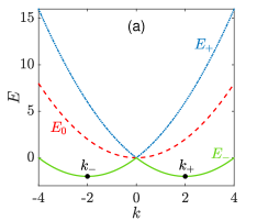
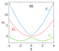
Figure 1: Three branches of the single-particle energy spectrum. (a) $p=0$. (b) $p=0.5$. Here $\gamma=2$ and $q=0$. $k_{\pm}$ are the momentum values corresponding to the two local minimums of $E_{-}$.

The two local minmums mean that the system has multiple stationary states. When all atoms in the BEC occupy a single momentum ($k_{+}$ or $k_{-}$), the system behaves as the PW phase. In particular, it behaves as the zero momentum phase when the single momentum is zero. Besides, when atoms occupy two momentums ($k_{+}$ and $k_{-}$), the state of system belongs to the SW phase.

Comparing Eqs. (3a) and (3b), $p$ and $q$ have similar effects on the modification of energy spectrum structure, and the influence of $p$ is shown in Fig. 1. As long as the strength of $p$ and $q$ is relatively not too strong, they only shift the phase boundary between these phases, and not affect the essence of the phases [8]. We only consider the case of $q=0$ because $q$ is generally much smaller than $p$.

IV Matter wave solitons and their existence and stability domains

IV.1 Without a Zeeman field

Matter wave solitons exist in every branch of the single-particle energy spectrum, but the stability of the solitons in the higher branches is relatively weak. We will mainly consider the solitons corresponding to the lowest branch $E_{-}$. At first, we discuss the solitons in a spin-1 BEC with SOC in the absence of Zeeman field $(p=0)$. In this case, Eq. (1) degenerate into the Nonlinear Schrödinger equation by some transformations [31], which is a integrable equation and has various exact solutions [48]. The Nonlinear Schrödinger equation is

$$i\frac{\partial u}{\partial t}+\frac{1}{2}\frac{\partial^{2}u}{\partial x^{2}}+\sigma|u|^{2}u=0,$$ (4)

where $u$ is the complex function of $x$ and $t$, and $\sigma=\pm 1$ represent attractive and repulsive interactions, respectively. The key transformations between Eqs. (1) and (4) are

$$\left(\begin{array}[]{c}\psi_{+1}\\ \psi_{0}\\ \psi_{-1}\end{array}\right) =\frac{e^{\frac{i}{2}\gamma^{2}t\pm i\gamma x}}{2\sqrt{g_{p}/\sigma}}u\left(\begin{gathered}1\\ \mp\sqrt{2}\\ 1\end{gathered}\right),$$ (5g)

$$\left(\begin{array}[]{c}\psi_{+1}\\ \psi_{0}\\ \psi_{-1}\end{array}\right) =\frac{e^{\frac{i}{2}\gamma^{2}t}}{2\sqrt{g_{s}/\sigma}}u\left(\begin{gathered}e^{i\gamma x}\pm e^{-i\gamma x}\\ -\sqrt{2}\left(e^{i\gamma x}\mp e^{-i\gamma x}\right)\\ e^{i\gamma x}\pm e^{-i\gamma x}\end{gathered}\right).$$ (5n)

Here, $g_{p}=-\left(c_{0}+c_{2}\right)$ and $g_{s}=-2c_{0}$. We notice that there are two PWs ($e^{\pm i\gamma x}$) in these transformations. In addition, the momentums $k_{\pm}$ corresponding to the local minimums of lowest branch are equal to $\pm\gamma$ in the absence of Zeeman field. It means Eqs. (5g) and (5n) represent the wave functions of the atoms occupying a single momentum and two momentums, respectively. Therefore, they correspond to the exact solutions of the PW phase and the SW phase of Eq. (1).

In the absence of Zeeman field, we can obtain a lot of exact analytical solutions. We are mainly concerned about the stationary-state solutions, especially the bright solitons. Thus we consider the attractive interaction ($\sigma=1$), and a bright soliton solution of Eq. (4) is

$$u=k_{1}{\rm sech}\left(k_{1}\left(x-vt\right)\right)e^{ivx+i\left(k_{1}^{2}-v^{2}\right)t/2},$$ (6)

where $k_{1}$ and $v$ are real parameters, which are the amplitude and velocity of the bright soliton, respectively. Substituting Eq. (6) into Eqs. (5g) and (5n), we derive four types of bright solitons which are the stationary states when $v=0$. Drawing the profiles at $t=0$, as shown in Fig. 2. We clearly observe their structures and differences. In Figs. 2 and 2, the PW solitons (PW1 and PW2, respectively) have bell-shaped structures and their component densities $n_{j}$ are the same. In addition, the SW solitons in Figs. 2 and 2 (SW1 and SW2, respectively) have stripe structure which is unique and concerned in systems with SOC. As we know, the functions of a stationary state about $x$ and $t$ can be separated, and the functions of $x$ and $t$ are $\varphi_{j}(x)$ and $e^{-i\mu t}$, respectively. Here, $\mu$ is the chemical potential, and we derive the chemical potentials of the four solitons $\mu=-\left(k_{1}^{2}+\gamma^{2}\right)/2$. Additionally, the local minimums of $E_{-}$ are all $-\gamma^{2}/2$. Therefore, we conclude that the widths and amplitudes of bright solitons are determined by the difference between the local minimum of energy spectrum and $\mu$. In fact, this is a universal law that holds true in other systems.

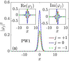
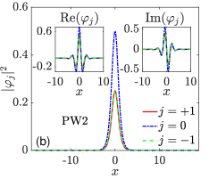
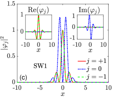
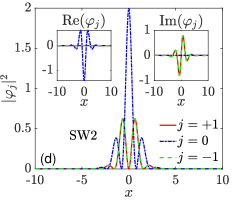
Figure 2: The four types of stationary bright solitons when $p=0$. The plane wave solitons (PW1, PW2) for $c_{0}=0.5$, $c_{2}=-1.5$ are in (a) and (b). The standing wave solitons (SW1, SW2) for $c_{0}=-0.5$, $c_{2}=1.5$ are in (c) and (d). The left and right subgraphs represent the real and imaginary parts of the solitons, respectively. Here, $k_{1}=1$ and $\gamma=2$.

With the exact solutions of PW1, PW2, SW1, and SW2 solitons, we can analyze conveniently their existence and stability domains. As we know, the attractive interaction is necessary for bright solitons. Therefore, $c_{0}+c_{2}<0$ and $c_{0}<0$ are the necessary conditions to form PW solitons and SW solitons, respectively. Of course, $k_{1}$ must be a real number, so $\mu<-\gamma^{2}/2$. For the stability of the stationary solitons $\varphi_{j}(x)$, there are two methods to analyze it, one is the evolution of the stationary solitons with small perturbations, and the other is the linear stability analysis. The latter is more suitable for analyzing the stability of a large number of stationary solitons. We consider adding small perturbations to the stationary solutions $\varphi_{j}(x)$ as follows:

$$\psi_{j}(x,t)=\left[\varphi_{j}(x)+a_{j}(x)e^{\lambda t}+b_{j}^{*}(x)e^{\lambda^{*}t}\right]e^{-i\mu t},$$ (7)

where $a_{j}$ and $b_{j}$ ($j=\pm 1,0$) are perturbation functions, $\lambda$ is the growth rate of the perturbations, and “$\ast$” denotes complex conjugation. Substituting the perturbed solutions into Eq. (1) and linearizing, we obtain an eigenvalue equation about perturbation functions $i\bm{L}\bm{\xi}=\lambda\bm{\xi}$, where $\bm{\xi}=[a_{+1},b_{+1},a_{0},b_{0},a_{-1},b_{-1}]^{T}$, and $T$ represents transposition. $\bm{L}$ is a matrix, and its matrix elements are given in Appendix A. By numerical calculations, we can obtain the eigenvalues of matrix $i\bm{L}$. When the real part maximum of $\lambda$ is greater than $10^{-3}$, we think that the stationary solutions are unstable because of the exponential growth of perturbations with time. Based on the linear stability analysis, we analyze the stability of PW and SW solitons in their existence domains, as shown in Fig. 3.

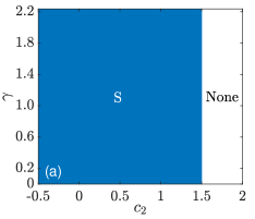
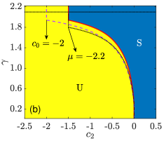
Figure 3: The stability domains of PW solitons (a) and SW solitons (b) about $c_{2}$ and $\gamma$. The blue (yellow) areas are stable (unstable) areas. PW solitons can not exist in white areas. Here, $\mu=-2.5$ and $c_{0}=-1.5$. The red solid line in (b) is the boundary between stable and unstable areas. Besides, the purple dashed line and the black dotted line represent the boundary when $c_{0}=-2$ and $\mu=-2.2$, respectively. In particular, the upper boundary of SW solitons becomes $\gamma=\sqrt{4.4}$ (the black horizontal line) when $\mu=-2.2$.

We find that the stability domains of PW1 and PW2 solitons are the same, as well as for SW1 and SW2 solitons. For PW solitons, they are all stable in the existence domain ($c_{2}<-c_{0}$ and $\gamma<\sqrt{-2\mu}$), as shown in Fig. 3. However, not all SW solitons are stable. Interestingly, $c_{2}$ does not affect the expressions of SW solitons solutions, but affects their stability, as shown in Fig. 3. According to the changes of the boundary between stable and unstable areas for different $c_{0}$ and $\mu$, we summarize some laws about the stability of SW solitons. When $c_{2}>0$ ($c_{2}<c_{0}$), the SW solitons are stable (unstable). In addition, there are stable and unstable SW solitons in the area of $c_{0}<c_{2}<0$, which is divided by a curve. The curve intersects with the straight line $c_{2}=c_{0}$. We find the abscissa and ordinate of the intersection point depend on $c_{0}$ and $\mu$, respectively. In short, SW (PW) solitons exist stably in all antiferromagnetic (ferromagnetic) and partial ferromagnetic (antiferromagnetic) areas. Decreasing the interaction $c_{0}$ results in a larger stable ferromagnetic (antiferromagnetic) area.

Next we discuss the moving solitons ($v\neq 0$) which are the stationary solutions in the moving frame. Although the Galilean invariance of Eq. (1) is broken by the SOC effect, we can get the moving solitons by coordinate transformations

$$x^{\prime}=x-vt,~{}~{}t^{\prime}=t,$$ (8)

$$\frac{\partial}{\partial x}=\frac{\partial}{\partial x^{\prime}},~{}~{}\frac{\partial}{\partial t}=\frac{\partial}{\partial t^{\prime}}-v\frac{\partial}{\partial x^{\prime}}.$$

Substituting Eq. (8) into Eq. (1), we obtain the equations in the moving frame. The details are in Appendix A. In the moving frame, the lowest branch becomes

$$E_{-}=\frac{k^{2}}{2}-vk-\sqrt{\gamma^{2}k^{2}}.$$ (9)

We find $v$ breaks the axial symmetry of energy spectrum, and the existence domains of PW and SW solitons are also changed. For PW solitons, the exact solutions obtained by Eqs. (5g) and (6) are still the stationary solutions in the moving frame. Similarly, we gain the chemical potentials $\mu_{1,2}=-\left(\gamma\pm v\right)^{2}/2-k_{1}^{2}/2$ corresponding to PW1 and PW2 solitons. When $\mu$ is fixed, the velocities of PW solitons are limited, the ranges of PW1 and PW2 solitons are $-\sqrt{-2\mu}\mp\gamma<v<\sqrt{-2\mu}\mp\gamma$, respectively. As shown in Fig. 4, the area is divided by four rays which are determined by $\mu$.

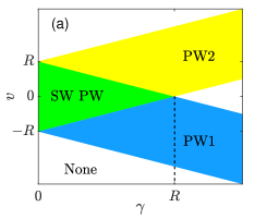
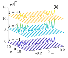
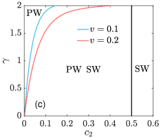
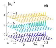
Figure 4: (a) The existence domains of moving PW and SW solitons about $\gamma$ and $v$. The bule (yellow) area is the existence domain of PW1 (PW2) solitons. All four types of bright solitons exist in the green area, but not in the white areas. Here, $R=\sqrt{-2\mu}$. (b) The three-component densities when $\mu=-2.5$, $\gamma=2.1$, $c_{0}=-0.5$, $c_{2}=0.3$, and $-0.3<v<0.3$. (c) The existence domains of moving PW and SW solitons about $\gamma$ and $c_{2}$ when $\mu=-2.5$ and $c_{0}=-0.5$. The blue solid (red dotted) line represents the dividing line when $v=0.1$ ($v=0.2$). The black solid line is the vanishing boundary of PW solitons. (d) The three-component densities corresponding to (c) for different $c_{2}$ when $\gamma=2$ and $v=0.1$. $|\varphi_{+1}|^{2}$ and $|\varphi_{0}|^{2}$ shown in (b) and (d) are translated.

PW1 and PW2 solitons exist in the blue and yellow areas, respectively. The green area is the common area of the blue and yellow areas, where both PW1 and PW2 solitons exist. For SW solitons, the exact solutions obtained by Eqs. (5n) and (6) is no longer applicable, we need to rely on numerical calculations (the squared-operator iteration method). We find SW solitons only exist in the green area, and the amplitudes of the SW solitons near the boundary of the green area are close to zero. Additionally, the limited range of the velocities of SW solitons is $-\sqrt{-2\mu}+\gamma<v<\sqrt{-2\mu}-\gamma$, which decreases as the increase of $\gamma$. Taking SW1 solitons as an example, selecting parameters $\mu=-2.5$, $c_{0}=-0.5$, and $c_{2}=0.3$, we show the three component densities when $\gamma=2.1$ in Fig. 4. We clearly observe that there are only PW solitons and no SW solitons when the absolute value of velocity is larger than $\sqrt{5}-2.1$.

In addition to $\gamma$ and $v$, $c_{0}$ and $c_{2}$ are also important parameters affecting the existence domains of moving solitons, as shown in Fig. 4. For PW solitons, $c_{2}+c_{0}<0$ is still the existence condition of moving PW solitons. But for SW solitons, $c_{2}$ can not be taken arbitrarily. SW solitons are limited to the right area of the blue solid (red dotted) curve on the plane ($c_{2},\gamma$) when $v=0.1$ ($v=0.2$). For example, noting the profiles of SW1 solitons when $\mu=-2.5$, $\gamma=2$, $c_{0}=-0.5$, and $v=0.1$, as shown in Fig. 4. We find the stripe contrast of the SW1 solitons become smaller as $c_{2}$ decreases, and the phase transition occurs when $c_{2}<0.155$. In a word, moving PW and SW solitons have a common area surrounded by the straight line $c_{2}=-c_{0}$ and a curve determined by $v$. In addition, moving PW and SW solitons also exist on the left and right of the common area, respectively. When $v<0$, the existence domain of SW solitons is consistent with that of $|v|$.

By discussing the stability of moving solitons in the existence domains, we find that the moving PW and SW solitons are all stable. Comparing Fig. 4 with Figs. 3 and 3, this is understandable because the moving solitons only exist in the stable area of the stationary solitons.

IV.2 With a Zeeman field

For the case that the Zeeman field exists ($p\neq 0$), $\psi_{+1}$ and $\psi_{-1}$ in Eq. (1) are no longer equivalent. It is difficult to obtain exact analytical solutions, so we choice the numerical method to find PW and SW solitons of Eq. (1), including moving and stationary solitons. In addition, we only consider the case of $p>0$ because it is symmetrical with the case of $p<0$.

We still analyze from the perspective of energy spectrum. In the moving frame, the lowest branch becomes

$$E_{-}=\frac{k^{2}}{2}-vk-\sqrt{\gamma^{2}k^{2}+p^{2}}.$$ (10)

$v$, $\gamma$ and $p$ affect the number of local minimums of $E_{-}$, which determines the types of solitons in the system. In addition, we know that $\gamma$ is the only reason why $E_{-}$ has a double-valley structure. Drawing $E_{-}$ for different $v$ and $p$, as shown in Fig. 5.

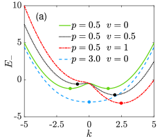
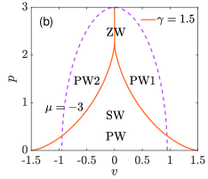
Figure 5: (a) The lowest branch $E_{-}$ of energy spectrum for different $v$ and $p$. The points represent the local minimums. Here, $\gamma=1.5$. (b) The existence domains of different types of solitons divided by the orange solid lines on the plane $(v,p)$ when $\gamma=1.5$. The purple dotted line represents the contour line with $\min(E_{-})=-3$. The existence condition of bright solitons is $\mu<\min(E_{-})$.

We find that the increase of $p$ causes $k_{+}$ and $k_{-}$ to approach each other, and the two local minimums to decrease. $v$ makes one of the local minimums increase and the other decrease. Whether $v$ or $p$ become large enough, the double-valley structure of $E_{-}$ is broken. In this case, there are only PW solitons and no SW solitons in the system. Basing on the number of local minimums of $E_{-}$, we obtain the existence domains of different types of solitons. As shown in Fig. 5, the orange solid lines determined by $\gamma$ divide the plane ($v,p$) into three areas when $\gamma=1.5$. Zero momentum solitons only exist in the case of $p>\gamma^{2}$ and $v=0$, except in this case, there are always PW solitons present. SW solitons exist in the area with small absolute values of $p$ and $v$. When $\mu$ is fixed, these bright solitons only exist in the semi-ellipse area surrounded by the purple dashed line. The larger $\mu$, the smaller the semi-ellipse area. Next, we mainly discuss PW and SW solitons.

Firstly, we obtain PW solitons in the existence domains and discuss their stability by numerical calculations. The necessary condition is $c_{0}+c_{2}<0$. when $v=0$, the stability domains of PW1 and PW2 solitons are completely consistent because of the symmetrical energy spectrum. By the control variable method, we systematically investigate the influence of various parameters on the stability of PW solitons, as shown in Figs. 6 and 6.

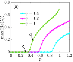
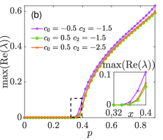
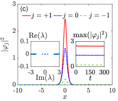
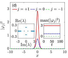
Figure 6: The influence of $p$ on the stability of PW solitons for different $\gamma$ (a) or for different $c_{0}$ and $c_{2}$ (b). (a) $c_{0}=0.5$ and $c_{2}=-1.5$. (b) $\gamma=1$. The subgraph in (b) is an enlarged view of the dashed frame. Here, $\mu=-2.5$ and $v=0$. (c) and (d) show the PW solitons in (a) when $p=0.3$ and $p=0.45$, respectively. Besides, the left and right subgraphs represent the linear stability analysis and the evolution of $\max(|\varphi_{j}|^{2})$ under 2% random-noise perturbations, respectively.

We find a commonality that the stable and unstable areas are separated by a critical value $p_{0}$. When $p$ is greater (small) than $p_{0}$, the corresponding PW soliton is unstable (stable). $p_{0}$ becomes larger with increasing $\gamma$. However, in the case of $c_{2}<0$, $p_{0}$ hardly changes when we adjust $c_{0}$ and $c_{2}$. It indicates that the stability of PW solitons is related to the single-particle energy spectrum. In addition, we give two examples to illustrate the correctness of the linear stability analysis, as shown in Figs. 6 and 6. We find $p$ makes the proportion of the three component densities change and affects the stability. During the real-time evolution of solitons with initial perturbations, the amplitudes of stable ($p=0.3$) and unstable ($p=0.45$) PW solitons remain unchanged and oscillate periodically, respectively, which is consistent with the results of the linear stability analysis.

We also discuss the influence of velocity on the stability of PW1 and PW2 solitons. As shown in Figs. 7 and 7, we find an interesting phenomenon that $v$ has opposite influence on the stability of PW1 and PW2 solitons. In other words, the critical values $p_{0}$ of the PW1 solitons ($v>0$) and the PW2 solitons ($v<0$) are all larger than that of the PW solitons ($v=0$). Besides, we find that the promoting effect of $v$ on stability is stronger than the inhibition effect.

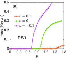
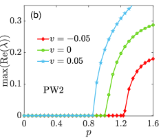
Figure 7: The influence of $p$ on the stability of PW1 solitons (a) and PW2 solitons (b) for different $v$. Here, $\mu=-2.5$, $\gamma=1.5$, $c_{0}=0.5$, and $c_{2}=-1.5$.

Combining the influence of $\gamma$, $c_{0}$, and $c_{2}$ on stability, we find the parameters which change the structure of $E_{-}$ significantly affect the stability of PW solitons, such as $\gamma$, $p$, and $v$. Further, when the curvature at the local minimum point of $E_{-}$ is small than one critical value, the corresponding PW soliton is unstable. The critical curvature is greatly impacted by $\gamma$, $v$, and $p$, but less impacted by $c_{0}$ and $c_{2}$ when $c_{2}<0$.

For the stability of SW solitons, we consider the case of $v=0$ firstly. In addition to the condition $p<\gamma^{2}$, $c_{0}<0$ is also a premise for the existence of SW solitons. From Fig. 3, we know that SW solitons are unstable in the absence of Zeeman field when $c_{2}<c_{0}$. Therefore, we focus on discussing the stability of SW solitons for $c_{2}>c_{0}$ when $p\neq 0$. In Fig. 8, the stable (blue) and unstable (yellow) areas of SW1 solitons are arranged alternately. When adjusting $c_{0}$ from $-0.5$ to $-1$, the dividing lines between stable and unstable areas change from the red solid lines to the black dashed lines.

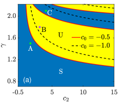
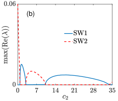
Figure 8: (a) The stability domains of SW1 solitons on the plane ($c_{2},\gamma$) for different $c_{0}$. The blue and yellow areas are stable and unstable areas of SW1 solitons, respectively, but for SW2 solitons, the opposite is true. The red solid lines are the dividing lines when $c_{0}=-0.5$. Besides, the dividing lines move to the black dashed lines when $c_{0}=-1$. The coordinates of three markers $\mathrm{A}$, $\mathrm{B}$, and $\mathrm{C}$ are $(1.5,1.5)$, $(3,1.8)$, and $(4,2.1)$, respectively. (b) The real part maximums of $\lambda$ for different $c_{2}$ when $\gamma=2.1$ and $c_{0}=-0.5$. The blue solid line and the red dashed line correspond to SW1 and SW2 solitons, respectively. Here, $\mu=-2.5$ and $p=0.5$.

Moreover, we find that SW1 solitons are all stable when $c_{0}<c_{2}<0$, which is caused by $p\neq 0$. It is different from the situation without a Zeeman field. The stability of SW2 solitons on the plane ($c_{2},\gamma$) is also analyzed. Coincidentally, the stability domains of SW1 and SW2 solitons are complementary. In other words, SW2 solitons are unstable in the stable areas of SW1 solitons. As shown in Fig. 8, we can clearly understand the complementarity, by observing the change of the real part maximum of $\lambda$ when $c_{2}$ increases. In addition, the alternating changes of the stability domains are not just twice. SW1 (SW2) solitons are stable (unstable) again when $c_{2}=34$. Thus, when $c_{2}$ continues to increase, there are still alternate stable and unstable areas. The instability of the unstable areas gradually weaken.

Selecting the parameters corresponding to $\mathrm{A}$, $\mathrm{B}$, and $\mathrm{C}$ in Fig. 8, we draw the profiles and stability of the corresponding SW1 and SW2 solitons, and show their evolutions, as shown in Fig. 9.

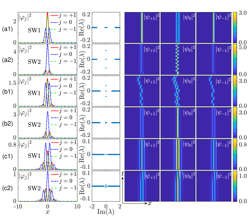
Figure 9: The profiles, stability, and evolution of the SW1 (odd rows), and SW2 solitons (even rows). The parameters of (a1) and (a2), (b1) and (b2), (c1) and (c2) correspond to $\mathrm{A}$, $\mathrm{B}$, $\mathrm{C}$ in Fig. 8, respectively. The first and second columns on the left represent the profile and stability of SW solitons, respectively. The three columns on the right represent the evolution of the three components under 2% random-noise perturbations, their transverse windows $x\in\left[-10,10\right]$ and longitudinal windows $t\in\left[0,1000\right]$. Besides, the colorbars for each row are shared.

We find the stability of the SW1 and SW2 solitons is indeed opposite, and the SW solitons with lower unstable growth rates can remain stable for longer time. However, the unstable SW solitons do not immediately disperse after deformation, they begin to change their profiles regularly. The reason is that the nonlinear terms in the Hamiltonian of Eq. (1) are equivalent to a time-dependent external potential when the SW solitons are unstable. The time-dependent external potential cause the quantum transport phenomena [49], which is similar to the unstable evolution in Fig. 9.

When $v\neq 0$, SW solitons are limited to the right area of the blue (red) curve in Fig. 10 when $v=0.1$ ($v=0.2$). Different from the situation without the Zeeman field, the linear Zeeman effect $p$ relax this restriction.

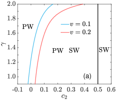
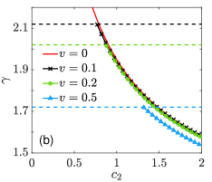
Figure 10: (a) The existence domains of moving PW and SW solitons for different $v$ when $p=0.5$. The blue solid (red dotted) line represents the dividing line when $v=0.1$ ($v=0.2$). The black solid line is the vanishing boundary of PW solitons. Here, $\mu=-2.5$ and $c_{0}=-0.5$. (b) The changes of the leftmost dividing line in Fig. 8 when $v\neq 0$. The dashed lines represent the upper boundaries of the existence domains of SW solitons at different velocities.

Comparing with Fig. 4, we find the existence domain of moving SW solitons expands slightly to the right when $p\neq 0$, and even contains a small portion of ferromagnetic area ($c_{2}<0$) when $v=0.1$. For the stability of moving SW solitons, $v$ only causes slight movement of the dividing lines of stability domain, especially when $v$ is small. As shown in Fig. 10, we only show the changes of the leftmost dividing line in Fig. 8 to observe clearly.

V Collision dynamics of stable solitons

The existence of stable moving solitons raises the question about their interactions. As we konw, when the relative velocity of two solitons is large, interference fringes are generated in the collision area [50]. Here, we only discuss the collisions between moving solitons with small velocities, and concentrate on the dynamics of the total particle density $n$ and $z$-component spin density $F_{z}=|\psi_{+1}|^{2}-|\psi_{-1}|^{2}$.

Selecting two solitons with opposite velocities in the stable areas and putting them in different positions, we find some interesting collision phenomena, as shown in Fig. 11.

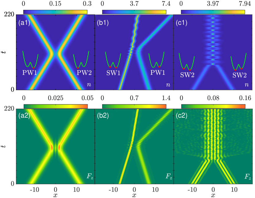
Figure 11: The collisions between different types of solitons. (a1-c1) and (a2-c2) display the evolution of the total particle density $n$ and the $z$-component spin density $F_{z}$, respectively. The subgraphs show the lowest branch $E_{-}$ and the corresponding local minimums of solitons. Here, $\mu=-2.5$, $\gamma=2$, $c_{0}=-0.5$, and $p=0.5$, but for the SW1 soliton in (b1) $\mu=-3.5$. The other parameters are $c_{2}=-1.5$, $v=\pm 0.1$ in (a1) and (a2), $c_{2}=0.2$, $v=\pm 0.05$ in (b1) and (b2), $c_{2}=3$, $v=\pm 0.1$ in (c1) and (c2).

In the two left figures, the PW1 and PW2 solitons bounce apart from each other after colliding, which occupy the minimums of their corresponding $E_{-}$ respectively. There are no transferred particles between the two solitons, but particles transfer between three components, as can be seen from the increase of $F_{z}$ after colliding. In addition, the collision between the PW2 and PW1 solitons which occupy the larger local minimums makes $F_{z}$ decrease, not shown here. Then noting the collision between the SW1 and PW1 solitons with different chemical potential $\mu$ in the two middle figures, we find the macroscopic tunneling effects [51, 52] near the collision area. After colliding, the SW1 soliton begins to oscillate periodically, and the velocity of the PW1 soliton changes. The $z$-component spin densities $F_{z}$ of the two solitons also begin to oscillate slightly. Furthermore, the most interesting phenomenon occurs in the collision between the two SW2 solitons in the right figures. The two SW2 solitons attract each other as they approach, leading to quasi-periodic collisions, during which a small portion of particles scatter and detach from the main body. $F_{z}$ still maintains a relatively good stripe shape after colliding. After more discussion, we find this phenomenon can also occur in the collision between two SW1 solitons with equal chemical potential $\mu$.

VI Conclusions

In summary, we investigated the stationary and moving bright solitons in spin-1 BECs with SOC in a Zeeman field. Combining the single-particle energy spectrum, exact solutions and numerical solutions, we systematically analyzed the existence and stability domains of four types of bright solitons (PW1, PW2, SW1, and SW2 solitons). Moreover, we briefly discussed the collision dynamics of different types of stable solitons, and found some interesting inelastic collision phenomena. We have summarized some laws about existence and stability of PW and SW solitons.

For the existence of PW and SW solitons, we find that the single-particle energy spectrum contains a lot of useful information. According to its local minimums, we can obtain the range of the chemical potential $\mu$ corresponding to solitons. By discussing the number of the local minimums, we can predict accurately the type of solitons which exist in the system. PW solitons exist when the energy spectrum has one or more local minimums. SW solitons only exist when the energy spectrum has two local minimums. We further find the interactions $c_{0}$ and $c_{2}$ are also key factors affecting the existence of solitons, and the necessary conditions for the existence of PW and SW solitons are $c_{0}+c_{2}<0$ and $c_{0}<0$, respectively. In particular, for moving SW solitons, $c_{2}$ is restricted and must be greater than zero. Fortunately, the linear Zeeman effect $p$ can relax this restriction and make the moving SW solitons exist in a small portion of antiferromagnetic areas ($c_{2}<0$).

For the stability of PW and SW solitons in the existence domains, we summarize the influence of various parameters on stability. In the absence of the Zeeman field, all stationary and moving PW solitons in the existence domain are stable. Stationary SW solitons stably exist in the ferromagnetic area ($c_{2}>0$) and a small portion of the antiferromagnetic area ($c_{2}<0$), but moving SW solitons are only stable in the ferromagnetic area because of the limitation of $c_{2}$. When $p\neq 0$, the stable areas vary greatly. For PW solitons, when $p>p_{0}$, the PW soliton are unstable. The parameters which change the curvature at the local minimum point significantly affect the stability of the corresponding PW soliton, such as $\gamma$, $p$, and $v$. Increasing the curvature at the local minimum point make the corresponding PW soliton more stable. Other parameters barely affect the stability of PW solitons, which do not change the curvature, such as $c_{0}$ and $c_{2}$. For SW solitons, the linear Zeeeman effect $p$ makes it impossible for both SW1 and SW2 solitons to exist stably under the same conditions. Their stable areas are complementary and staggered on the plane ($c_{2},\gamma$). SW1 solitons are even stable in the ferromagnetic area where SW1 solitons are unstable when $p=0$. Adjusting $c_{0}$ by the Feshbach resonance technology, we can change the stability of SW solitons. Moreover, we find $v$ slightly affects stability of SW solitons. The stable areas of the moving SW solitons with small velocity and the stationary SW solitons are almost the same.

Appendix A The equations and the linear stability analysis in the moving frame

By coordinate transformations Eq. (8), we obtain the equations describing a spin-orbit-coupled spin-1 BEC in the moving frame

$${i}\frac{\partial\psi_{+1}}{\partial{t}} =\left(-\frac{1}{2}\frac{\partial^{2}}{\partial{x}^{2}}+c_{0}n+c_{2}\left(n_{+1}+n_{0}-n_{-1}\right)\right)\psi_{+1}$$ (11)

$$+ c_{2}\psi_{0}^{2}\psi_{-1}^{*}-\frac{i\gamma}{\sqrt{2}}\frac{\partial\psi_{0}}{\partial x}+(q-p)\psi_{+1}+iv\frac{\partial\psi_{+1}}{\partial x},$$

$${i}\frac{\partial\psi_{0}}{\partial{t}} =\left(-\frac{1}{2}\frac{\partial^{2}}{\partial{x}^{2}}+c_{0}n+c_{2}\left(n_{+1}+n_{-1}\right)\right)\psi_{0}$$

$$+ 2c_{2}\psi_{0}^{*}\psi_{+1}\psi_{-1}-\frac{i\gamma}{\sqrt{2}}\left(\frac{\partial\psi_{+1}}{\partial x}+\frac{\partial\psi_{-1}}{\partial x}\right)+iv\frac{\partial\psi_{0}}{\partial x},$$

$${i}\frac{\partial\psi_{-1}}{\partial{t}} =\left(-\frac{1}{2}\frac{\partial^{2}}{\partial{x}^{2}}+c_{0}n+c_{2}\left(n_{-1}+n_{0}-n_{+1}\right)\right)\psi_{-1}$$

$$+ c_{2}\psi_{0}^{2}\psi_{+1}^{*}-\frac{i\gamma}{\sqrt{2}}\frac{\partial\psi_{0}}{\partial x}+(q+p)\psi_{-1}+iv\frac{\partial\psi_{-1}}{\partial x}.$$

Substituting $\psi_{j}(x,t)=\varphi_{j}(x)e^{-i\mu t}$ into Eq. (11), we obtain the stationary state equations,

$$\mu\varphi_{+1} =\left(-\frac{1}{2}\frac{\partial^{2}}{\partial{x}^{2}}+c_{0}n+c_{2}\left(n_{+1}+n_{0}-n_{-1}\right)\right)\varphi_{+1}$$ (12)

$$+ c_{2}\varphi_{0}^{2}\varphi_{-1}^{*}-\frac{i\gamma}{\sqrt{2}}\frac{\partial\varphi_{0}}{\partial x}+(q-p)\varphi_{+1}+iv\frac{\partial\varphi_{+1}}{\partial x},$$

$$\mu\varphi_{0} =\left(-\frac{1}{2}\frac{\partial^{2}}{\partial{x}^{2}}+c_{0}n+c_{2}\left(n_{+1}+n_{-1}\right)\right)\varphi_{0}$$

$$+ 2c_{2}\varphi_{0}^{*}\varphi_{+1}\varphi_{-1}-\frac{i\gamma}{\sqrt{2}}\left(\frac{\partial\varphi_{+1}}{\partial x}+\frac{\partial\varphi_{-1}}{\partial x}\right)+iv\frac{\partial\varphi_{0}}{\partial x},$$

$$\mu\varphi_{-1} =\left(-\frac{1}{2}\frac{\partial^{2}}{\partial{x}^{2}}+c_{0}n+c_{2}\left(n_{-1}+n_{0}-n_{+1}\right)\right)\varphi_{-1}$$

$$+ c_{2}\varphi_{0}^{2}\varphi_{+1}^{*}-\frac{i\gamma}{\sqrt{2}}\frac{\partial\varphi_{0}}{\partial x}+(q+p)\varphi_{-1}+iv\frac{\partial\varphi_{-1}}{\partial x}.$$

Both the stationary and moving solitons can be obtained by solving Eq. (12) numerically when the exact solutions are difficult to be obtained.

The following describes the steps of the linear stability analysis. Substituting the perturbed solutions Eq. (7) into Eq. (11) and linearizing, we obtain the equations about the perturbation functions

$$i\bm{L}\bm{\xi}=\lambda\bm{\xi},$$ (13)

where

$$\bm{L} =\left[\begin{array}[]{cccccc}L_{11}&L_{12}&L_{13}&L_{14}&L_{15}&L_{16}\\ L_{21}&L_{22}&L_{23}&L_{24}&L_{25}&L_{26}\\ L_{31}&L_{32}&L_{33}&L_{34}&L_{35}&L_{36}\\ L_{41}&L_{42}&L_{43}&L_{44}&L_{45}&L_{46}\\ L_{51}&L_{52}&L_{53}&L_{54}&L_{55}&L_{56}\\ L_{61}&L_{62}&L_{63}&L_{64}&L_{65}&L_{66}\end{array}\right],$$ (14)

$$\bm{\xi} =\left[a_{+1},b_{+1},a_{0},b_{0},a_{-1},b_{-1}\right]^{T}.$$

The matrix elements of $\bm{L}$ are

$$L_{11} =\frac{1}{2}\frac{\partial^{2}}{\partial x^{2}}+\mu+p-q-C_{+}\left(2n_{+1}+n_{0}\right)$$ (15)

$$- C_{-}n_{-1}-iv\frac{\partial}{\partial x},~{}L_{12}=-C_{+}\varphi_{+1}^{2},$$

$$L_{13} =\frac{i\gamma}{\sqrt{2}}\frac{\partial}{\partial x}-C_{+}\varphi_{0}^{*}\varphi_{+1}-2c_{2}\varphi_{-1}^{*}\varphi_{0},$$

$$L_{14} =-C_{+}\varphi_{0}\varphi_{+1},~{}L_{15}=-C_{-}\varphi_{-1}^{*}\varphi_{+1},$$

$$L_{16} =-C_{-}\varphi_{-1}\varphi_{+1}-c_{2}\varphi_{0}^{2},~{}L_{21}=C_{+}{\varphi_{+1}^{*}}^{2},$$

$$L_{22} =-\frac{1}{2}\frac{\partial^{2}}{\partial x^{2}}-\mu-p+q+C_{+}\left(2n_{+1}+n_{0}\right)$$

$$+ C_{-}n_{-1}-iv\frac{\partial}{\partial x},~{}L_{23}=C_{+}\varphi_{0}^{*}\varphi_{+1}^{*},$$

$$L_{24} =\frac{i\gamma}{\sqrt{2}}\frac{\partial}{\partial x}+C_{+}\varphi_{0}\varphi_{+1}^{*}+2c_{2}\varphi_{-1}\varphi_{0}^{*},$$

$$L_{25} =C_{-}\varphi_{-1}^{*}\varphi_{+1}^{*}+c_{2}{\varphi_{0}^{*}}^{2},~{}L_{26}=C_{-}\varphi_{-1}\varphi_{+1}^{*},$$

$$L_{31} =\frac{i\gamma}{\sqrt{2}}\frac{\partial}{\partial x}-C_{+}\varphi_{0}\varphi_{+1}^{*}-2c_{2}\varphi_{-1}\varphi_{0}^{*},$$

$$L_{32} =-C_{+}\varphi_{0}\varphi_{+1},$$

$$L_{33} =\frac{1}{2}\frac{\partial^{2}}{\partial x^{2}}+\mu-C_{+}\left(n_{+1}+n_{-1}\right)$$

$$- 2c_{0}n_{0}-iv\frac{\partial}{\partial x},~{}L_{34}=-2c_{2}\varphi_{-1}\varphi_{+1}-c_{0}\varphi_{0}^{2},$$

$$L_{35} =\frac{i\gamma}{\sqrt{2}}\frac{\partial}{\partial x}-C_{+}\varphi_{0}\varphi_{-1}^{*}-2c_{2}\varphi_{+1}\varphi_{0}^{*},$$

$$L_{36} =-C_{+}\varphi_{-1}\varphi_{0},~{}L_{41}=C_{+}\varphi_{+1}^{*}\varphi_{0}^{*},$$

$$L_{42} =\frac{i\gamma}{\sqrt{2}}\frac{\partial}{\partial x}+C_{+}\varphi_{+1}\varphi_{0}^{*}+2c_{2}\varphi_{0}\varphi_{-1}^{*},$$

$$L_{43} =2c_{2}\varphi_{-1}^{*}\varphi_{+1}^{*}+c_{0}{\varphi_{0}^{*}}^{2},$$

$$L_{44} =-\frac{1}{2}\frac{\partial^{2}}{\partial x^{2}}-\mu+C_{+}\left(n_{+1}+n_{-1}\right)$$

$$+ 2c_{0}n_{0}-iv\frac{\partial}{\partial x},~{}L_{45}=C_{+}\varphi_{-1}^{*}\varphi_{0}^{*},$$

$$L_{46} =\frac{i\gamma}{\sqrt{2}}\frac{\partial}{\partial x}+C_{+}\varphi_{-1}\varphi_{0}^{*}+2c_{2}\varphi_{0}\varphi_{+1}^{*},$$

$$L_{51} =-C_{-}\varphi_{+1}^{*}\varphi_{-1},~{}L_{52}=-C_{-}\varphi_{-1}\varphi_{+1}-c_{2}\varphi_{0}^{2},$$

$$L_{53} =\frac{i\gamma}{\sqrt{2}}\frac{\partial}{\partial x}-C_{+}\varphi_{0}^{*}\varphi_{-1}-2c_{2}\varphi_{+1}^{*}\varphi_{0},$$

$$L_{54} =-C_{+}\varphi_{0}\varphi_{-1},$$

$$L_{55} =\frac{1}{2}\frac{\partial^{2}}{\partial x^{2}}+\mu-p-q-C_{+}\left(2n_{-1}+n_{0}\right)$$

$$- C_{-}n_{+1}-iv\frac{\partial}{\partial x},~{}L_{56}=-C_{+}\varphi_{-1}^{2},$$

$$L_{61} =C_{-}\varphi_{-1}^{*}\varphi_{+1}^{*}+c_{2}{\varphi_{0}^{*}}^{2},$$

$$L_{62} =C_{-}\varphi_{+1}\varphi_{-1}^{*},~{}L_{63}=C_{+}\varphi_{0}^{*}\varphi_{-1}^{*},$$

$$L_{64} =\frac{i\gamma}{\sqrt{2}}\frac{\partial}{\partial x}+C_{+}\varphi_{0}\varphi_{-1}^{*}+2c_{2}\varphi_{+1}\varphi_{0}^{*},$$

$$L_{65} =C_{+}{\varphi_{-1}^{*}}^{2},~{}L_{66}=-\frac{1}{2}\frac{\partial^{2}}{\partial x^{2}}-\mu+p+q$$

$$+ C_{+}\left(2n_{-1}+n_{0}\right)+C_{-}n_{+1}-iv\frac{\partial}{\partial x}.$$

Here, $C_{+}=c_{0}+c_{2}$ and $C_{-}=c_{0}-c_{2}$. Then we transform the Eq. (14) into the momentum space, and solve the eigenvalues $\lambda$ numerically. We can judge the stability of solitons based on whether the real part maximum of $\lambda$ is greater than $10^{-3}$.

References

- [1] Y. J. Lin, K. J. García, and I. B. Spielman, Spin-orbit-coupled Bose-Einstein condensates, Nature 471, 83 (2011).
- [2] A. J. Leggett, Superfluidity, Rev. Mod. Phys. 71, S318 (1999).
- [3] Q.-J. Chena, J. Stajicb, S.-N. Tan, and K. Levin, BCS-BEC crossover: From high temperature superconductors to ultracold superfluids, Phys. Rep. 412, 1 (2005).
- [4] Y. A. Bychkov and E. I. Rashba, Oscillatory effects and the magnetic susceptibility of carriers in inversion layers, J. Phys. C 17, 6039 (1984).
- [5] G. Dresselhaus, Spin-orbit coupling effects in zinc blende structures, Phys. Rev. 100, 580 (1955).
- [6] X.-L. Qi and S.-C. Zhang, Topological insulators and superconductors, Rev. Mod. Phys. 83, 1057 (2011).
- [7] J. Sinova, S. O. Valenzuela, J. Wunderlich, C. H. Back, and T. Jungwirth, Spin Hall effects, Rev. Mod. Phys. 87, 1213 (2015).
- [8] C. J. Wang, C. Gao, C. M. Jian, and H. Zhai, Spin-Orbit Coupled Spinor Bose-Einstein Condensates, Phys. Rev. Lett. 105, 160403 (2010).
- [9] T.-L. Ho and S.-Z. Zhang, Bose-Einstein Condensates with Spin-Orbit Interaction, Phys. Rev. Lett. 107, 150403 (2011).
- [10] L. Wen, Q. Sun, H. Q. Wang, A. C. Ji, and W. M. Liu, Ground state of spin-1 Bose-Einstein condensates with spin-orbit coupling in a Zeeman field, Phys. Rev. A 86, 043602 (2012).
- [11] Z.-H. Lan and P. Öhberg, Raman-dressed spin-1 spin-orbit-coupled quantum gas, Phys. Rev. A 89, 023630 (2014).
- [12] S. S. Natu, X.-P. Li, and W. S. Cole, Striped ferronematic ground states in a spin-orbit-coupled Bose gas, Phys. Rev. A 91, 023608 (2015).
- [13] K.-E. Sun, C.-L. Qu, Y. Xu, Y.-P. Zhang, and C.-W. Zhang, Interacting spin-orbit-coupled spin-1 Bose-Einstein condensates, Phys. Rev. A 93, 023615 (2016).
- [14] D. L. Campbell, R. M. Price, A. Putra, A. Valdés-Curiel, D. Trypogeorgos, and I. B. Spielman, Magnetic phases of spin-1 spin–orbit-coupled Bose gases, Nat. Commun. 7, 10897 (2016).
- [15] Y. Li, L. P. Pitaevskii, and S. Stringari, Quantum Tricriticality and Phase Transitions in Spin-Orbit Coupled Bose-Einstein Condensates, Phys. Rev. Lett. 108, 225301 (2012).
- [16] L. Chen, H. Pu, and Y.-b. Zhang, Spin-orbit angular momentum coupling in a spin-1 Bose-Einstein condensate, Phys. Rev. A 93, 013629 (2016).
- [17] K. Mæland, A. T. G. Janssønn, J. H. Rygh, and A. Sudbø, Plane- and stripe-wave phases of a spin-orbit-coupled Bose-Einstein condensate in an optical lattice with a Zeeman field, Phys. Rev. A 102, 053318 (2020).
- [18] Y.-Y. Chen, H. Lyu, Y. Xu, and Y,-P. Zhang, Elementary excitations in a spin–orbit-coupled spin-1 Bose–Einstein condensate, New J. Phys. 24 073041 (2022).
- [19] J.-R. Li, J. Lee, W.-J. Huang, S. Burchesky, B. Shteynas, F. Ç. Top, A. O. Jamison, and W. Ketterle, A stripe phase with supersolid properties in spin–orbit-coupled Bose–Einstein condensates, Nature 543, 91 (2017).
- [20] L. Wen, Q. Sun, Y. Chen, D.-S. Wang, J. Hu, H. Chen, W.-M. Liu, G. Juzeliūnas, B. A. Malomed, and A.-C. Ji, Motion of solitons in one-dimensional spin-orbit-coupled Bose-Einstein condensates, Phys. Rev. A 94, 061602 (2016).
- [21] Y. V. Kartashov, V. V. Konotop, D. A. Zezyulin, and L. Torner, Bloch Oscillations in Optical and Zeeman Lattices in the Presence of Spin-Orbit Coupling, Phys. Rev. Lett. 117, 215301 (2016).
- [22] X. Chai, D. Lao, K. Fujimoto, R. Hamazaki, M. Ueda, and C. Raman, Magnetic Solitons in a Spin-1 Bose-Einstein Condensate, Phys. Rev. Lett. 125, 030402 (2020).
- [23] Y. V. Kartashov, V. V. Konotop, M. Modugno, and E. Ya. Sherman, Solitons in Inhomogeneous Gauge Potentials: Integrable and Nonintegrable Dynamics, Phys. Rev. Lett. 122, 064101 (2019).
- [24] X. Qiu, A.-Y. Hu, Y.-Y Cai, H. Saito, X.-F. Zhang, and L. Wen, Dynamics of spin-nematic bright solitary waves in spin-tensor-momentum coupled Bose-Einstein condensates, Phys. Rev. A 107, 033308 (2023).
- [25] S. K. Adhikari, Phase separation of vector solitons in spin-orbit-coupled spin-1 condensates, Phys. Rev. A 100, 063618 (2019).
- [26] S. Gautam and S. K. Adhikari, Vector solitons in a spin-orbit-coupled spin-2 Bose-Einstein condensate, Phys. Rev. A 91, 063617 (2015).
- [27] Y. Xu, Y.-P. Zhang, and C.-W. Zhang, Bright solitons in a two-dimensional spin-orbit-coupled dipolar Bose-Einstein condensate, Phys. Rev. A 92, 013633 (2015).
- [28] S. Gautam and S. K. Adhikari, Vortex-bright solitons in a spin-orbit-coupled spin-1 condensate, Phys. Rev. A 95, 013608 (2017).
- [29] S. K. Adhikari, Multiring, stripe, and superlattice solitons in a spin-orbit-coupled spin-1 condensate, Phys. Rev. A 103, L011301 (2021).
- [30] S. K. Adhikari, Symbiotic solitons in quasi-one- and quasi-two-dimensional spin-1 condensates, Phys. Rev. E 104, 024207 (2021).
- [31] J.-T. He, P.-P. Fang, and J. Lin, Multi-Type Solitons in Spin-Orbit Coupled Spin-1 Bose–Einstein Condensates, Chin. Phys. Lett. 39, 020301 (2022).
- [32] G. C. Katsimiga, S. I. Mistakidis, K. Mukherjee, P. G. Kevrekidis, and P. Schmelcher, Stability and dynamics across magnetic phases of vortex-bright type excitations in spinor Bose-Einstein condensates, Phys. Rev. A 107, 013313 (2023).
- [33] Y.-E Li and J.-K. Xue, Moving Matter-Wave Solitons in Spin–Orbit Coupled Bose–Einstein Condensates, Chin. Phys. Lett. 33, 100502 (2016).
- [34] Y.-E Li and J.-K. Xue, Stationary and moving solitons in spin–orbit-coupled spin-1 Bose–Einstein condensates, Front. Phys. 13, 130307 (2016).
- [35] X.-X. Li, R.-J. Cheng, J.-L. Ma, A.-X. Zhang, and J.-K. Xue, Solitary matter wave in spin-orbit-coupled Bose-Einstein condensates with helicoidal gauge potential, Phys. Rev. E 104, 034214 (2021).
- [36] N.-S. Wan, Y.-E Li, and J.-K. Xue, Solitons in spin-orbit-coupled spin-2 spinor Bose-Einstein condensates, Phys. Rev. E 99, 062220 (2019).
- [37] Y. Xu, Y.-P. Zhang, and B. Wu, Bright solitons in spin-orbit-coupled Bose-Einstein condensates, Phys. Rev. A 87, 013614 (2013).
- [38] V. Achilleos, D. J. Frantzeskakis, P. G. Kevrekidis, and D. E. Pelinovsky, Matter-Wave Bright Solitons in Spin-Orbit Coupled Bose-Einstein Condensates, Phys. Rev. Lett. 110, 264101 (2013).
- [39] Y. V. Kartashov, V. V. Konotop, and D. A. Zezyulin, Bose-Einstein condensates with localized spin-orbit coupling: Soliton complexes and spinor dynamics, Phys. Rev. A 90, 063621 (2014).
- [40] Y. V. Kartashov and V. V. Konotop, Solitons in Bose-Einstein Condensates with Helicoidal Spin-Orbit Coupling, Phys. Rev. Lett. 118, 190401 (2017).
- [41] H. Sakaguchi, E. Y. Sherman, and B. A. Malomed, Vortex solitons in two-dimensional spin-orbit coupled Bose-Einstein condensates: Effects of the Rashba-Dresselhaus coupling and Zeeman splitting, Phys. Rev. E 94, 032202 (2016).
- [42] V. Zapf, M. Jaime, and C. D.Batista, Bose-Einstein condensation in quantum magnets, Rev. Mod. Phys. 86, 563 (2014).
- [43] D. Zhao, S.-W. Song, L. Wen, Z.-D. Li, H.-G. Luo, and W.-M. Liu, Topological defects and inhomogeneous spin patterns induced by the quadratic Zeeman effect in spin-1 Bose-Einstein condensates, Phys. Rev. A 91, 013619 (2015).
- [44] R. Ravisankar, H. Fabrelli, A. Gammal, P. Muruganandam, and P. K. Mishra, Effect of Rashba spin-orbit and Rabi couplings on the excitation spectrum of binary Bose-Einstein condensates, Phys. Rev. A 104, 053315 (2021).
- [45] J. Sun, Y.-Y. Chen, X. Chen, and Y.-P. Zhang, Bright solitons in a spin-tensor-momentum-coupled Bose-Einstein condensate, Phys. Rev. A 101, 053621 (2020).
- [46] M. Ueda and Y. Kawaguchi, Spinor Bose–Einstein condensates, Phys. Rep. 520, 253 (2012).
- [47] D. J. Papoular, G. V. Shlyapnikov, and J. Dalibard, Microwave-induced Fano-Feshbach resonances, Phys. Rev. A 81, 041603 (2010).
- [48] T. Kanna and M. Lakshmanan, Exact soliton solutions of coupled nonlinear Schrödinger equations: Shape-changing collisions, logic gates, and partially coherent solitons, Phys. Rev. E 67, 046617 (2003).
- [49] Q.-D. Fu, P. Wang, Y. V. Kartashov, V. V. Konotop, and F.-W. Ye, Nonlinear Thouless Pumping: Solitons and Transport Breakdown, Phys. Rev. Lett. 128, 154101 (2022).
- [50] J. L. Helm, S. L. Cornish, and S. A. Gardiner, Sagnac Interferometry Using Bright Matter-Wave Solitons, Phys. Rev. Lett. 114, 134101 (2015).
- [51] L.-C. Zhao, L.-M. Ling, Z.-Y. Yang, and W.-L. Yang, Tunneling dynamics between atomic bright solitons, Nonlinear Dyn. 88, 2957 (2017).
- [52] Q. Jia, H.-B. Qiu, and A. M. Mateo, Soliton collisions in Bose-Einstein condensates with current-dependent interactions, Phys. Rev. A 106, 063314 (2022).