Quasinormal mode spectrum of the AdS black hole with the Robin boundary condition

Abstract

We study the quasinormal mode (QNM) spectrum of an asymptotically AdS black hole with the Robin boundary condition at infinity. We consider the Schwarzshild-AdS₄ with the flat event horizon as the background spacetime and study its scalar field perturbation. Denoting leading coefficients of slow- and fast-decay modes of the scalar field at infinity as $\phi_{1}$ and $\phi_{2}$, respectively, we assume a linear relation between them as $\phi_{2}=\cot(\theta/2)\phi_{1}$, where $\theta$ is a constant called the Robin parameter and periodic under $\theta\sim\theta+2\pi$. In a certain range of the Robin parameter, there is an instability driven by the boundary condition. We also find the holonomy in the QNM spectrum under the parametric cycle of the boundary condition: $\theta=0\to 2\pi$. After the one-cycle, $n$-th overtone of the QNM moves to $(n-1)$-th overtone. The fundamental tone of the QNM is swept out to the infinity in the complex plane.

1 Introduction

Asymptotically AdS spacetimes have time-like boundary at infinity and are not globally hyperbolic. To determine the dynamics of a field in the asymptotically AdS spacetime, it is necessary to specify a boundary condition at the boundary as well as the initial condition. What boundary conditions are allowed at infinity? For concreteness, let us consider a massive free scalar field $\Phi$ satisfying $\Box\Phi=\mu^{2}\Phi$ in four dimensions. When the metric asymptotes to that of the Poincare AdS₄ as $ds^{2}\simeq(-dt^{2}+dz^{2}+dx^{2}+dy^{2})/z^{2}$ in the unit of AdS radius, the scalar field behaves as

$$\Phi(t,z,x,y)=z^{\Delta_{-}}(\phi_{1}(t,x,y)+\cdots)+z^{\Delta_{+}}(\phi_{2}(t,x,y)+\cdots)\ \quad(z\sim 0),$$ (1)

where $\Delta_{\pm}=3/2\pm\sqrt{9/4+\mu^{2}}$ and dots represent subleading terms determined by solving the equation of motion. We will call the first and second terms as slow- and fast-decay modes, respectively. One of the simplest choice of the boundary condition is $\phi_{1}=0$, i.e, there is no slow-decay mode. However, this is not unique choice. In Refs. Breitenlohner:1982jf ; ishibashi:2004wx , it has been shown that a finite energy can be defined even when $\phi_{1}\neq 0$ if the mass square is in

$$-\frac{9}{4}<\mu^{2}<-\frac{5}{4}\ .$$ (2)

Then, we can consider the more general boundary condition as

$$\phi_{2}=\kappa\phi_{1}\ .$$ (3)

For $\kappa=0$ and $\kappa=\pm\infty$, we simply have $\phi_{2}=0$ and $\phi_{1}=0$, respectively. We will call them as the Neumann and Dirichlet boundary conditions, respectively. For $\kappa\neq 0,\pm\infty$, We will call the above condition as the Robin boundary condition.

In the AdS/CFT correspondence Maldacena:1997re ; Gubser:1998bc ; Witten:1998qj , changing the boundary condition of the scalar field from Neumann to Robin corresponds to the double-trace deformation of the dual field theory Witten:2001ua ; Berkooz:2002ug ; Mueck:2002gm ; Minces:2002wp ; Sever:2002fk ; Gubser:2002vv ; Aharony:2005sh ; Elitzur:2005kz ; Hartman:2006dy ; Diaz:2007an ; Papadimitriou:2007sj . Thus, study of dynamics of the scalar field with the Robin boundary condition will be important for understanding the dynamics of the deformed theory.

Dynamics of the scalar field in asymptotically AdS spacetimes with the Robin boundary condition has been studied in several previous works. In Ref. Araneda:2016ecy , it was shown that there is an unstable mode for a sufficiently large negative value of $\kappa$ for general asymptotically AdS spacetimes. In Refs. Dappiaggi:2017pbe ; Ferreira:2017tnc ; Katagiri:2020mvm , the effect of the Robin boundary condition on the superradiant instability of rotating and charged black holes in AdS was studied. A nonlinear solitonic solution was also explicitly constructed under the Robin condition as a candidate of the final fate of the instability of the global AdS Bizon:2020yqs . In Ref. Harada:2023cfl , hairy charged black holes and charged boson stars under the Robin conditions were constructed and their phase structure has been revealed.

In this paper, we will focus on the quasinormal mode spectrum of the scalar field in the Schwarzschild-AdS₄ spacetime with the Robin boundary condition. If a black hole is perturbed, the perturbation will be dissipated into the horizon. The relaxation process of the black hole perturbation is characterized by a complex-valued eigenfrequency called the quasinormal mode (QNM) frequency Chandrasekhar:1975zza . (See Kokkotas:1999bd ; Berti:2009kk ; Konoplya:2011qq for reviews.) In the view of the AdS/CFT, certain asymptotically AdS black holes are considered as gravitational duals of thermal states in dual field theories and quasinormal mode spectra of AdS black holes have information about the equilibration of the thermal states Horowitz:1999jd . It has also been proposed that the QNM spectrum corresponds to poles of the retarded Green function of the thermal quantum field theory Birmingham:2001pj ; Son:2002sd ; Kovtun:2005ev . Especially, if there is an unstable mode in the gravitational theory, (i.e., if a QNM frequency is in the upper half of the complex plane), it indicates the instability of the thermal state and existence of a new stable phase in the dual field theory.

This paper is organized as follows. In section 2, we consider the ordinary wave equation in $(1+1)$ dimension with the Robin boundary condition as a toy example. Studying the normal mode spectrum, we explicitly show that there is an unstable mode for a certain window of the Robin parameter $\kappa$. In section 3, we study the QNM spectrum of the scalar field with the Robin boundary condition. We take the Schwarzschild-AdS₄ spacetime with flat horizon as the background. Section 4 is devoted to the conclusion. In appendix, the detail of the numerical computation of the QNM is summarized.

2 Toy example: ($1+1$)-d wave equation with Robin boundary condition

2.1 Spectrum

To understand the effect of the Robin boundary condition, we consider the wave equation in ($1+1$)-dimensional flat spacetime:

$$\ddot{\phi}-\phi^{\prime\prime}=0\ ,$$ (4)

where ${}^{\cdot}\equiv\partial_{t}$ and ${}^{\prime}\equiv\partial_{x}$. We take the domain of the wave equation as $0\leq x\leq 1$. We impose the Robin boundary condition at $x=0$ and the Dirichlet one at $x=1$ as

$$\phi^{\prime}|_{x=0}=\kappa\phi|_{x=0}\ ,$$ (5)

$$\phi|_{x=1}=0\ ,$$ (6)

where $\kappa\in\mathbb{R}$ represents the Robin parameter: $\kappa=0$ and $\kappa=\pm\infty$ correspond to the Neumann and Dirichlet boundary conditions, respectively. For the following analysis, it is convenient to introduce a parameter $\theta$ as

$$\kappa=\cot\frac{\theta}{2}\ .$$ (7)

In terms of $\theta$, the Dirichlet and Neumann boundary conditions correspond to $\theta=0$ and $\theta=\pi$. The Robin boundary condition are specified by a point on the circle as in Fig. 1. For any value of $\theta$, we have a trivial solution $\phi=0$. We will study the spectrum of the scalar field $\phi$ with conditions (5) and (6). In Bizon:2020yqs , it has been shown that the Klein-Gordon equation for spherically symmetric scalar field in the global AdS₄ reduces to Eq. (4) and instability has been found for certain Robin boundary conditions. (See also  Araneda:2016ecy for the case of semi-infinite domain, $0\leq x<\infty$.)

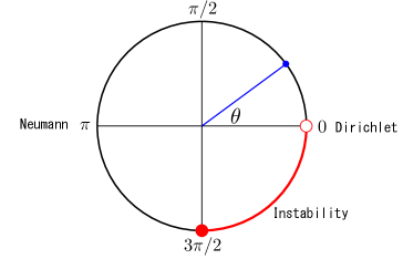
Figure 1: Visualization of parameter space for the Robin boundary conditions ($\kappa=\cot(\theta/2)$). The Dirichlet and Neumann boundary conditions are given by $\theta=0$ and $\theta=\pi$, respectively. On the portion of the circle shown by red, the trivial solution $\phi=0$ is unstable.

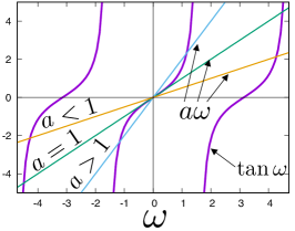
(a) $\omega\in\mathbb{R}$

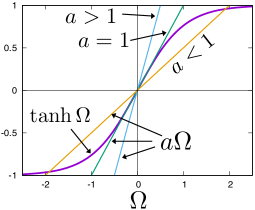
(b) $\omega\in i\mathbb{R}$  ($\omega\equiv i\Omega$)

Figure 2: Illustration for determining spectrum.

Let us consider a single mode whose frequency is $\omega$. By only imposing the boundary condition (6) at $x=1$, we have a solution of the wave equation as

$$\phi(t,x)=e^{-i\omega t}\sin\omega(1-x)\ .$$ (8)

Substituting the above expression into the Robin boundary condition (5) at $x=0$, we obtain an equation which determines the spectrum:

$$a\omega=\tan\omega\ ,\qquad(a\equiv-\tan\frac{\theta}{2})\ .$$ (9)

For the Dirichlet ($\theta=0$) and Neumann ($\theta=\pi$) conditions, the spectra are given by $\omega_{n}=n\pi$ $(n\in\mathbb{Z}\backslash\{0\})$ and $\omega_{n}=(n+1/2)\pi$ ($n\in\mathbb{Z}$), respectively. Although, for a general value of $\theta$, we cannot obtain analytical solutions, we can see the $\theta$-dependence of the spectrum graphically Bizon:2020yqs . Figure 2(a) shows each side of Eq. (9) as functions of $\omega\in\mathbb{R}$. The intersections correspond to the spectrum given by Eq. (9). In the region of $|\omega|<\pi/2$, the number of intersections depends on the slope of the linear function, $a=-\tan(\theta/2)$. Imagine that we start from $a>1$ and decrease the value of $a$. Initially, there are three intersections in $|\omega|<\pi/2$. For $a=1$, however, all the three intersections merge at $\omega=0$. For $a<1$, we only have single intersection at the origin. The critical case $a=1$ corresponds to $\theta=3\pi/2$. Where have lost two solutions gone to? They have gone to the complex plane. To see this, we assume that the frequency $\omega$ is pure imaginary and denote $\omega=i\Omega$. Then, Eq. (9) is rewritten as

$$a\Omega=\tanh\Omega\ .$$ (10)

Figure 2(b) shows each side of Eq. (10) as functions of $\Omega$. For $a<1$, we can find two pure imaginary solutions. The mode with $\textrm{Im}\,\omega>0$ grows exponentially in $t$ and implies instability of the trivial solution $\phi=0$. Figure 3 shows the motion of eigenfrequencies on the complex $\omega$-plane when we change the value of $\theta$ from $0$ to $2\pi$. For the Dirichlet condition $\theta=0$, all eigenfrequencies are located at the red points on the real axis. For the critical case $\theta=3\pi/2$, two of the eigenfrequencies merge at the origin. For $\theta>3\pi/2$, they split into the the imaginary axis and the unstable mode appears. For the Dirichlet condition after the one-cycle, $\theta=2\pi$, the two eigenfrequencies on the imaginary axis swept out to the infinity and this is consistent with the stability of the trivial solution for the Dirichlet condition. By the one-cycle $\theta=0\to 2\pi$, normal mode frequencies move as $\omega_{n+1}\to\omega_{n}$ $(n\geq 1)$ and $\omega_{n-1}\to\omega_{n}$ $(n\leq-1)$. The fundamental mode frequencies go to infinity $\omega_{\pm 1}\to\pm\infty i$ for $\theta\to 2\pi$. It follows that we have the same distributions of normal mode frequencies for $\theta=2\pi m$ ($m\in\mathbb{Z}$). When the eigenfrequency is pure imaginary $\omega=i\Omega$, the mode function becomes

$$\phi=ie^{\Omega t}\sinh\Omega(1-x)\ .$$ (11)

This function is localized at $x\sim 0$ for a sufficiently large $\Omega$. In the limit $\Omega\to\pm\infty$, this becomes singular eventually.

For the critical case $\theta=3\pi/2$, we can explicitly find the solution of the wave equation:

$$\phi(t,x)=Ct(1-x)\ ,$$ (12)

where $C$ is an arbitrary constant. This grows linearly in $t$. Thus, $\theta=3\pi/2$ is marginally unstable. In summary, the condition for instability of the trivial solution $\phi=0$ with the Robin boundary is given by

$$\frac{3}{2}{\pi}\leq\theta<2\pi\ \quad\left(\kappa\leq-1\right).$$ (13)

The unstable boundary conditions are illustrated in Fig. 1.

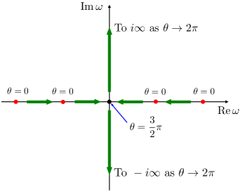
Figure 3: Motion of eigenfrequencies in the complex $\omega$-plane.

2.2 Origin of instability

We have seen that the ordinary wave equation is unstable when the inequality (13) is satisfied. The unstable mode grows exponentially and should have a larger energy at the late time comparing to that of the initial state. Where did the energy come from? We give an energetics of the instability in this subsection.

We can naively define the Hamiltonian of the current system as

$$H=\frac{1}{2}\int_{0}^{1}\!\!dx\,[\dot{\phi}^{2}(t,x)+\phi^{\prime 2}(t,x)].$$ (14)

Its time derivative is

$$\frac{dH}{dt} =\int_{0}^{1}\!\!dx\,[\dot{\phi}(t,x)\ddot{\phi}(t,x)+\phi^{\prime}(t,x)\dot{\phi}^{\prime}(t,x)]$$ (15)

$$=\int_{0}^{1}\!\!dx\,\frac{\partial}{\partial x}[\dot{\phi}(t,x)\phi^{\prime}(t,x)]$$

$$=-\dot{\phi}(t,0)\phi^{\prime}(t,0),$$

where we have imposed the Dirichlet condition $\phi=0$ at the other side $x=1$. This means that the energy cannot be always conserved due to a flux injected from the boundary depending on the boundary condition at $x=0$. Now, at $x=0$, we consider the Robin boundary condition: $\phi(t,0)\cos(\theta/2)-\phi^{\prime}(t,0)\sin(\theta/2)=0$. Then, we have

$$\frac{dH}{dt}=-\cot\frac{\theta}{2}\,\phi(t,0)\dot{\phi}(t,0)=-\frac{d}{dt}\left(\frac{\cot(\theta/2)}{2}\phi^{2}(t,0)\right)\ .$$ (16)

Thus, it turns out that the “modified” Hamiltonian

$$\tilde{H}=\frac{1}{2}\int_{0}^{1}\!\!dx\,[\dot{\phi}^{2}(t,x)+\phi^{\prime 2}(t,x)]+\frac{1}{2}\phi^{2}(t,0)\cot(\theta/2)$$ (17)

is conserved under the Robin condition. The integral of the above expression is clearly non-negative. On the other hand, the last term can be negative depending on the sign of $\cot(\theta/2)$. Only if the Robin parameter is negative, $\kappa=\cot(\theta/2)<0$ ($\pi<\theta<2\pi$), this system can be unstable in which $\phi(t,x)$ would be unbounded. This consideration is consistent with results in the previous subsection.

Let us now carefully consider the boundary term of the action. An action that provides the wave equation (4) is simply given by

$$S[\phi]=\int^{t_{2}}_{t_{1}}\!\!dt\int_{0}^{1}\!\!dx\,\frac{1}{2}[\dot{\phi}^{2}(t,x)-\phi^{\prime 2}(t,x)].$$ (18)

Its first variation for $\phi+\delta\phi$ becomes

$$\delta S =\int^{t_{2}}_{t_{1}}\!\!dt\int_{0}^{1}\!\!dx\,[\dot{\phi}\delta\dot{\phi}-\phi^{\prime}\delta\phi^{\prime}]$$ (19)

$$=\int^{t_{2}}_{t_{1}}\!\!dt\,\phi^{\prime}(t,0)\delta\phi(t,0),$$

where we have used the equation of motion. The first variation of the original action $S$ does not always vanish with respect to an arbitrary variation $\delta\phi$ at $x=0$. We define an action with a total derivative term as

$$\widetilde{S} \equiv S-\frac{\cot(\theta/2)}{2}\int^{t_{2}}_{t_{1}}\!\!dt\,\phi^{2}(t,0)$$ (20)

$$=S+\cot\frac{\theta}{2}\int^{t_{2}}_{t_{1}}\!\!dt\int_{0}^{1}\!\!dx\,\phi(t,x)\phi^{\prime}(t,x).$$

We note that this modified action $\widetilde{S}$ can satisfy $\delta\widetilde{S}=0$ with respect to an arbitrary variation $\delta\phi$ at $x=0$ imposing the Robin boundary condition. We consider the invariance of the action in terms of time translation $t\to t+\epsilon$. The Noether theorem states that a conserved charge exists on shell. What we emphasize is that it relies on use of the boundary conditions as well as the equations of motion. Under the Robin boundary condition, the variation of the modified action yield no boundary contribution, so that the Noether charge derived from $\widetilde{S}$ can be conserved without any flux on the boundary.

From the modified Lagrangian density:

$$\widetilde{\mathcal{L}}=\frac{1}{2}[\dot{\phi}^{2}-\phi^{\prime 2}]+\cot\frac{\theta}{2}\,\phi\phi^{\prime},$$ (21)

we have the Hamiltonian density:

$$\widetilde{\mathcal{H}}=\frac{1}{2}[\pi^{2}+\phi^{\prime 2}]-\cot\frac{\theta}{2}\,\phi\phi^{\prime}\quad\left(\pi\equiv\frac{\partial\widetilde{\mathcal{L}}}{\partial\dot{\phi}}=\dot{\phi}\right).$$ (22)

This provides a conserved energy in this system as

$$\tilde{H}=\int^{1}_{0}dx\widetilde{\mathcal{H}}=\frac{1}{2}\int^{1}_{0}dx[\dot{\phi}^{2}+\phi^{\prime 2}]+\frac{1}{2}\cot\frac{\theta}{2}\phi(t,0)^{2}.$$ (23)

Thus, we can reproduce Eq. (17) as the conserved quantity again.

In fact, the boundary condition at $x=0$ locally causes the two pure imaginary modes that we have seen previously. To understand it easily, let us consider the following one-dimensional Schödinger problem:

$$\left[-\frac{d^{2}}{dx^{2}}+2\kappa\delta(x)\right]\phi_{\omega}(x)=\omega^{2}\phi_{\omega}(x).$$ (24)

Integrating it within $-\epsilon\leq x\leq\epsilon$, we have

$$-\left.\frac{d}{dx}\phi_{\omega}(x)\right|^{\epsilon}_{-\epsilon}+2\kappa\phi_{\omega}(0)=0,$$ (25)

which provides the Robin boundary condition, $\phi^{\prime}_{\omega}(0)=\kappa\phi_{\omega}(0)$, at $x=0$. This means that imposing the Robin boundary condition at $x=0$ is equivalent to adding to the delta-function potential at $x=0$, whose coefficient is determined by $\kappa$.

Now, we will focus on local behavior near $x=0$ irrelevant to boundary condition at the other side. Imposing outgoing boundary conditions $\phi_{\omega}(x)\sim\exp(+i\omega x)$ for $x\to\infty$ and $\phi_{\omega}(x)\sim\exp(-i\omega x)$ for $x\to-\infty$, a solution is

$$\phi_{\omega}(x)=c\exp(\kappa|x|),\quad\omega=\pm i\kappa.$$ (26)

If $\kappa<0$, this solution describes a bound state with $\omega^{2}<0$ by the delta potential well. It turns out that the existence of the “bound state with delta potential” is origin of the instability under the Robin boundary condition with negative Robin parameters.

3 QNM spectrum of the scalar field with the Robin boundary condition

3.1 Setup

We consider the four-dimensional Schwarzschild-AdS spacetime (Sch-AdS₄) with the flat horizon as the background spacetime,

$$ds^{2}=\frac{l^{2}}{z^{2}}\quantity(-F(z)dt^{2}+\frac{1}{F(z)}dz^{2}+dx^{2}+dy^{2})\ ,\quad F(z)=1-\frac{z^{3}}{z_{h}^{3}},$$ (27)

where $l$ is the AdS radius and the event horizon is located at $z=z_{h}$. This metric satisfies the Einstein equation in vacuum: $G_{\mu\nu}-3l^{-2}{g_{\mu\nu}}=0$. From now on, we use the system of units with $l=z_{h}=1$. In the ingoing Eddington-Finkelstein (EF) coordinates $(v,z)$, the metric (27) can be rewritten as

$$ds^{2}=\frac{1}{z^{2}}(-F(z)dv^{2}-2dvdz+dx^{2}+dy^{2}),$$ (28)

where

$$v=t+r_{*},\quad r_{*}=-\int^{z}_{0}\frac{d\tilde{z}}{F(\tilde{z})}.$$ (29)

Note that the tortoise coordinate $r_{*}$ behaves as $r_{*}\simeq-z$ and $r_{*}\to-\infty$ near the AdS boundary ($z\sim 0$) and the horizon ($z=1$), respectively.

We consider the Klein-Gordon equation

$$\Box\Phi-\mu^{2}\Phi=0,$$ (30)

in the Sch-AdS₄ spacetime. The scalar field $\Phi$ can be expanded by Fourier modes as

$$\Phi(v,z,x,y)=\varphi(z)e^{-i\omega v+i\mathbf{k}\cdot\mathbf{x}}=\phi(z)e^{-i\omega t+i\mathbf{k}\cdot\mathbf{x}},$$ (31)

where $\varphi(z)$ and $\phi(z)$ are Fourier coefficients in $(v,z)$- and $(t,z)$-coordinates, respectively. Note that, since $\phi(z)=\varphi(z)e^{-i\omega r_{\ast}}$, we have

$$\phi(z)\simeq\varphi(z)(1+i\omega z)\quad(z\simeq 0).$$ (32)

Substituting Eq. (31) into the Klein-Gordon equation (30), we obtain the equation for $\varphi(z)$ as

$$-\mu^{2}\varphi+z\left[-(k^{2}z+2i\omega)\varphi+(2iz\omega-2F+zF^{\prime})\varphi^{\prime}+zF\varphi^{\prime\prime}\right]=0,$$ (33)

where ${}^{\prime}\equiv d/dz$.

Now, for simplicity, we consider that the mass square is

$$\mu^{2}=-2\ .$$ (34)

In this case, the asymptotic form of the solution of the equation (33) at $z\sim 0$ is given by

$$\varphi(z)\sim\varphi_{1}z+\varphi_{2}z^{2}\ ,\qquad\phi(z)\sim\phi_{1}z+\phi_{2}z^{2}.$$ (35)

Then, from Eq. (32), the above coefficients are related to each other as follows:

$$\phi_{1}=\varphi_{1}\ ,\quad\phi_{2}=\varphi_{2}+i\omega\varphi_{1}.$$ (36)

Imposing the Robin boundary condition (3) in the $(t,z)$-coordinates, we obtain

$$\varphi_{2}+i\omega\varphi_{1}=\kappa\varphi_{1},$$ (37)

in the ingoing EF coordinates. For later convenience, we introduce the rescaled variable as

$$f(z)\equiv\frac{\varphi(z)}{z}\sim\varphi_{1}+\varphi_{2}z.$$ (38)

From Eqs. (33), (34), and (38), in terms of $f(z)$ the field equation can be rewritten as

$$-(k^{2}+z)f(z)+(2\lambda-3z^{2})f^{\prime}(z)+(1-z^{3})f^{\prime\prime}(z)=0,$$ (39)

where $\omega=-i\lambda$. The Robin boundary condition (37) is also written as

$$f^{\prime}(0)+(\lambda-\kappa)f(0)=0.$$ (40)

Furthermore, in order to obtain QNMs, we should impose the ingoing boundary condition on the scalar field at the horizon. Because of formulating in the ingoing EF coordinates, we just have to require $f(z)$ to be regular at the future horizon $z=1$. Thus, if we obtain $\lambda$ and $f(z)$ that satisfy the above equations, the QNM spectrum and mode functions can be determined.

In later calculations, we mainly use the periodic parameter $\theta$ defined by equation (7) instead of $\kappa$ as the Robin parameter. We can take its domain as $0\leq\theta<2\pi$ without loss of generality. Note that $\theta=0$ ($\kappa=\pm\infty$) corresponds to the Dirichlet boundary condition, while $\theta=\pi$ ($\kappa=0$) corresponds to the Neumann boundary condition. For simplicity, we set the wave number $k=0$, that is, we will focus on homogeneous modes.

3.2 The results of QNM spectrum and mode functions

In this subsection, we will show our numerical results on QNM spectra with the Robin boundary condition. We have used the spectral method for the numerical calculations. See appendix A for details. Figures 4(a)-4(c) show the QNM spectra for $\theta=0$ (Dirichlet), $\pi$ (Neumann), and $7\pi/4$ (Robin). From these figures, we can see that the QNM spectra depends on the Robin parameter $\theta$ and, especially, an unstable mode appears for $\theta=7\pi/4$. Figure 4(d) shows the imaginary part of QNM frequencies as the function of the Robin parameter $\theta$.

Figure 5 shows the trajectory of the QNM frequencies in the complex plane for one cycle of the Robin parameter $\theta=0\to 2\pi$. The blue points show the QNM spectrum for the Dirichlet condition $\theta=0$. Let $n$ denote the tone number and its QNM frequency be $\omega_{n}$ (Re $\omega_{n}\geq 0)$. Note that $\omega^{\prime}_{n}\equiv-\omega_{n}^{\ast}$ is also a QNM frequency. First, we track the change of the fundamental frequencies $\omega_{0}$ and $\omega^{\prime}_{0}$ for $\theta=0\to 2\pi$. As the value of $\theta$ is gradually increasing from $0$, both $\omega_{0}$ and $\omega^{\prime}_{0}$ approach the imaginary axis. At $\theta\simeq 1.18\pi$, they merge at the point A on the imaginary axis. As $\theta$ is further increasing, they split into two modes on the imaginary axis, and in the limit of $\theta\to 2\pi$, each mode asymptotically approaches $\pm\infty i$. On the other hand, tracking overtones $\omega_{n}$ and $\omega^{\prime}_{n}$ ($n\geq 1$), we find that they move to the positions of the QNM frequencies with one lower overtone number: $\omega_{n}\to\omega_{n-1}$ and $\omega_{n}^{\prime}\to\omega^{\prime}_{n-1}$ for $\theta=0\to 2\pi$. After one cycle $\theta=0\to 2\pi$, the distribution of the QNM spectrum returns to its original one but, if we focus on tracking each QNM frequency, it never returns to its original position. In this sense, there is holonomy in the parametric cycle $\theta=0\to 2\pi$.

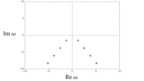
(a) QNM spectrum for $\theta=0$

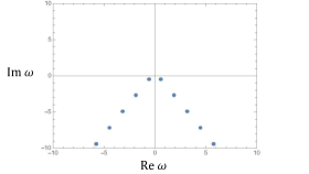
(b) QNM spectrum for $\theta=\pi$

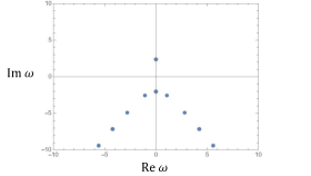
(c) QNM spectrum for $\theta=7\pi/4$

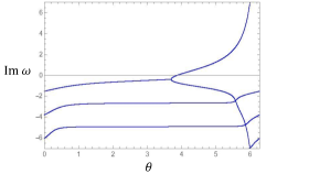
(d) Imaginary part of QNM frequencies

Figure 4: (a)-(c) QNM spectra for $0$ (Dirichlet), $\theta=\pi$ (Neumann), $7\pi/4$ (Robin). (d) $\theta$ dependence of the imaginary part of the QNM frequencies.

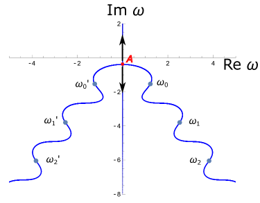
Figure 5: The trajectory of quasinormal frequencies with respect to the Robin parameter $\theta$.

Figure 6 shows the real and imaginary parts of mode functions with the fundamental tone for various Robin parameters $\theta=m\pi/3$ ($m=0,1,\ldots,5$). We have normalized the mode functions as $f(0)=1$ and $f^{\prime}(0)=1$ for $\theta\neq 0$ and $\theta=0$, respectively. Note that the mode function becomes a real function when $\omega$ is pure imaginary.

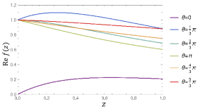
(a) Re$f(z)$

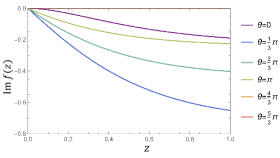
(b) Im$f(z)$

Figure 6: Mode functions of the fundamental tone for $\theta=\pi m/3$, ($m=0,1,2,\cdots 5$).

As in Figure 5, we find that the QNM frequencies of the fundamental tones have swept out to infinity as $\omega\to\pm\infty i$ $(\lambda\to\pm\infty)$ in the limit of $\theta\to 2\pi-0$. Thus, for $\theta\simeq 2\pi-0$, supposing $|\lambda|\gg 1$, the principal part of differential equation (39) can be approximately written as $\lambda f^{\prime}(z)\simeq 0$, and then its solution is given by $f(z)=\textrm{const.}$ In fact, the mode function approaches a constant as $\theta\to 2\pi-0$ as shown in Fig. 6(a).

3.3 Onset of the instability

As one can see in Figure 4(d), the unstable mode appears depending on the Robin parameter $\theta$. To consider the onset of instability, we substitute $\omega=0$ into Eq. (39) and solve the second-order differential equation. The general solution is given by

$$f(z)=c_{1}\ {}_{2}F_{1}\quantity(\frac{1}{3},\frac{1}{3};\frac{2}{3};z^{3})+c_{2}z\ _{2}F_{1}\quantity(\frac{2}{3},\frac{2}{3};\frac{4}{3};z^{3}),$$ (41)

where ${}_{2}F_{1}(a,b;c;z)$ is the Gaussian hypergeometric function. Each of the hypergeometric functions diverges logarithmically at $z\rightarrow 1$. In order for the solution to be regular at $z=1$, we will choose the coefficients $c_{1}$ and $c_{2}$ so as to cancel out the terms of $\log(1-z)$ in the two hypergeometric functions. As the result, we have

$$f(z)=f_{0}(z) \equiv{}_{2}F_{1}\quantity(\frac{1}{3},\frac{1}{3};\frac{2}{3};z^{3})-\frac{3\Gamma(2/3)^{3}}{\Gamma(1/3)^{3}}z\,{}_{2}F_{1}\quantity(\frac{2}{3},\frac{2}{3};\frac{4}{3};z^{3})$$ (42)

$$=\frac{\Gamma(2/3)^{2}}{\Gamma(1/3)}{}_{2}F_{1}\quantity(\frac{1}{3},\frac{1}{3};1;1-z^{3}),$$

where we have chosen an overall coefficient as $f(0)=1$. The above function is shown in Fig. 7. From Eq. (42), the Robin parameter at the onset of instability can be read out by (40) as

$$\kappa=\frac{f^{\prime}_{0}(0)}{f_{0}(0)}=-\frac{3\Gamma(2/3)^{3}}{\Gamma(1/3)^{3}}\simeq-0.3874.$$ (43)

Also, the value of $\theta=2\,\textrm{arccot}\,\kappa$ at the onset of instability is given by $\theta\simeq 1.235\pi\simeq 222.4^{\circ}$. Therefore, the range of $\theta$ where the instability occurs is

$$222.4^{\circ}\simeq 2\,\textrm{arccot}\left(-\frac{3\Gamma(2/3)^{3}}{\Gamma(1/3)^{3}}\right)\leq\theta<360^{\circ}.$$ (44)

At the onset of instability (43), we can find that $\Phi(t,z)=tzf_{0}(z)$ is an exact solution of the Klein-Gordon equation. It follows that the Sch-AdS₄ is marginally unstable at the onset.

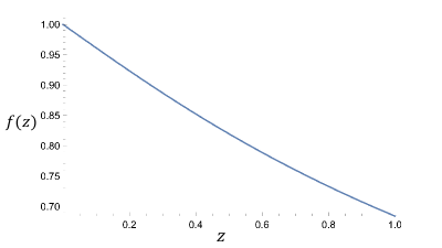
Figure 7: The mode function at the onset of the instability.

3.4 Origin of instability

In this subsection we argue origin of instability under the Robin boundary condition in asymptotically AdS spacetime as in Sec. 2.2. The renormalized action for a scalar field deHaro:2000vlm is given by

$$S[\Phi]=-\frac{1}{2}\int_{z\geq\epsilon}d^{4}x\sqrt{-g}\left(g^{\mu\nu}\nabla_{\mu}\Phi\nabla_{\nu}\Phi+\mu^{2}\Phi^{2}\right)-\frac{\Delta_{-}}{2l}\left.\int d^{3}x\sqrt{-h}\Phi^{2}\right|_{z=\epsilon},$$ (45)

where $h_{\mu\nu}$ denotes the induced metric on the AdS boundary $z=\epsilon$ for $\epsilon\to 0$. Note that the last term is a counter term for the action to regularize at the AdS boundary. In terms of $\Phi\to\Phi+\delta\Phi$, the variation of the action with imposing the field equation is

$$\delta S =\left.\int d^{3}x(\sqrt{-g}g^{zz}\Phi^{\prime}-l^{-1}\Delta_{-}\sqrt{-h}\Phi)\delta\Phi\right|_{z=\epsilon}$$ (46)

$$=\left.\int d^{3}x\sqrt{-h}(\sqrt{g^{zz}}\Phi^{\prime}-l^{-1}\Delta_{-}\Phi)\delta\Phi\right|_{z=\epsilon}$$

$$=l^{2}(\Delta_{+}-\Delta_{-})\left.\int d^{3}x\phi_{2}\delta\phi_{1}\right|_{z=\epsilon}.$$

Thus, the on-shell action depends on the boundary data of the scalar field $\phi_{1}$. To make the variation of the action vanish under the Robin boundary condition $\phi_{2}=\kappa\phi_{1}$, we should modify the action as

$$\widetilde{S}=S-l^{2}(\Delta_{+}-\Delta_{-})\int d^{3}x\frac{\kappa}{2}\phi_{1}^{2}.$$ (47)

The Hamiltonian derived from the action (45) is

$$H =\int dx^{2}\int dz\sqrt{-g}(-T^{0}{}_{0})+\frac{\Delta_{-}}{2l}\left.\int d^{2}x\sqrt{-h}\Phi^{2}\right|_{z=\epsilon},$$ (48)

where $T_{\mu\nu}$ is the minimal stress tensor for the scalar field given by

$$T_{\mu\nu}=\nabla_{\mu}\Phi\nabla_{\nu}\Phi-\frac{1}{2}g_{\mu\nu}\left(\nabla^{\rho}\Phi\nabla_{\rho}\Phi+\mu^{2}\Phi^{2}\right).$$ (49)

This is equivalent to the Killing energy with respect to the time-translational Killing vector $\xi^{\mu}$. The local conservation law for the stress tensor, $\nabla_{\mu}(T^{\mu\nu}\xi_{\nu})=0$, yields

$$\frac{d}{dt}H =\int d^{2}x\int_{0}^{z_{h}}dz\frac{\partial}{\partial t}(-\sqrt{-g}T^{0}{}_{0})+\frac{\Delta_{-}}{l}\left.\int d^{2}x\sqrt{-h}\Phi\dot{\Phi}\right|_{z=\epsilon}$$ (50)

$$=\left.\int d^{2}x\left(-\sqrt{-g}T^{z}{}_{0}+\frac{\Delta_{-}}{l}\sqrt{-h}\Phi\dot{\Phi}\right)\right|_{z=0}$$

$$=-\left.\int d^{2}x\sqrt{-h}\left(\sqrt{g^{zz}}\Phi^{\prime}-\frac{\Delta_{-}}{l}\Phi\right)\dot{\Phi}\right|_{z=0}$$

$$=-l^{2}(\Delta_{+}-\Delta_{-})\int d^{2}x\phi_{2}\dot{\phi}_{1}.$$

It turns out that the Hamiltonian is conserved if the Dirichlet condition $\phi_{1}=0$ or the Neumann condition $\phi_{2}=0$ satisfies, while it cannot be conserved otherwise. Indeed, when we impose the Robin boundary condition $\phi_{2}=\kappa\phi_{1}$, the energy flux appears at the AdS boundary.

Now, we define the modified energy, corresponding to the Noether charge derived from the modified action $\widetilde{S}$, as

$$E_{\text{mod}} \equiv H+l(\Delta_{+}-\Delta_{-})\frac{\kappa}{2}\int d^{2}x\phi_{1}^{2}$$ (51)

$$=\int dx^{2}\int dz\sqrt{-g}(-T^{0}{}_{0})+\frac{\Delta_{-}}{2l}\left.\int d^{2}x\sqrt{-h}\Phi^{2}\right|_{z=\epsilon}$$

$$\quad+l(\Delta_{+}-\Delta_{-})\frac{\kappa}{2}\int d^{2}x\phi_{1}^{2},$$

which can be conserved at the AdS boundary under the Robin boundary condition $\phi_{2}=\kappa\phi_{1}$. Since $\Delta_{+}-\Delta_{-}=\sqrt{9+\mu^{2}}>0$, if $\kappa<0$, $\Phi$ could be unbounded with the modified energy kept conserved. As in the case of the $(1+1)$-wave equation, the Robin boundary condition with negative $\kappa$ works as if infinite energy is stored at the AdS boundary.

It is worth noting that the modified action and energy discussed above is related to the double-trace deformation of the boundary CFT in the context of the AdS/CFT correspondence. In order for the variation problem of the bulk action to be well-defined, the action is chosen so that the contribution of the boundary term should vanish under the Robin boundary condition for the bulk field. Then, the energy defined by the Noether charge for that action will be conserved and such action and energy are identical to the ones discussed here on shell.

4 Conclusion

We investigated the QNM spectrum of scalar fields on Sch-AdS₄ imposing the Robin boundary condition. As a result, as can be seen from Figure 5 and Figure 4(d), after the parametric cycle of the Robin parameter, $\theta=0\to 2\pi$, while the spectrum itself does not change, the fundamental tone is swept out to the infinity in the complex plane and the $n$-th overtone moves to the $(n-1)$-th overtone for $n\geq 1$. In this sense, there is holonomy under the cycle $\theta=0\to 2\pi$. We also found the unstable mode for the scalar field perturbation under the Robin boundary condition with $222.4^{\circ}\leq\theta<360^{\circ}$. Furthermore, we numerically obtained the $\theta$ dependence of the mode function of the fundamental tone.

This instability arises from the Robin boundary condition with negative $\kappa$. The origin can be intuitively understood as follows. The Robin boundary condition with negative $\kappa$ corresponds to a delta-function potential well and can work as an infinite energy storage. Indeed, under the Robin boundary conditions, the conserved energy as Noether charge is modified by adding a boundary contribution, whose sign depends on the Robin parameter $\kappa$. As a result, when $\kappa$ is negative, the ordinary bulk energy of the scalar field could be unbounded while the modified energy remains constant. We can expect that this type of instability commonly exists for probe fields in asymptptically AdS spacetimes.

For $\theta=2\pi$ or $\theta=0$, the boundary condition is just Dirichlet and there is no instability. On the other hand, for $\theta=2\pi-\epsilon$ ($0<\epsilon\ll 1$), which corresponds to a Robin boundary condition with an extremely large negative $\kappa$, the growth rate of instability has an extremely large value, whereas the instability does not occur for $\theta=\epsilon$. (In terms of delta-function potentials, the Robin boundary condition for $\theta=2\pi-\epsilon$ corresponds to a very deep potential well and that for $\theta=\epsilon$ to a very high potential barrier. Thus, in real time dynamics of the scalar field, we might be able to think that the unstable mode dominates in an instant for $\theta=2\pi-\epsilon$. Does the tiny change of the boundary condition significantly change the real time dynamics of the scalar field? The study of the real time dynamics of the scalar field with the Robin boundary condition is an interesting future direction. We might have to take into account the “excitation factor” Berti:2006wq to understand dynamics of the scalar field under the Robin boundary condition.

We found the instability of the Sch-AdS₄ under the scalar field perturbation with the Robin boundary condition. At the onset of the instability, there is the static perturbation as in Eq. (42). We can expect that there is a family of nonlinear solutions branching off from the onset. Explicit construction of such hairy black hole solutions would be the other future direction.

Appendix A Detail of the numerical calculation of the QNM

We describe the detail of the numerical method to compute the QNM spectrum. This method is based on the Yaffe’s Mathematica notebook in the Mathematica Summer School on Theoretical Physics Yaffe . In the notebook, the spectral method is used to solve the eigenvalue problem for differential equations.

We introduce the Chebyshev polynomial as

$$T_{n}(x)\equiv\cos(n\arccos{x})\qquad(n=0,1,2,\ldots).$$ (52)

The Chebyshev polynomials form a complete orthogonal system of functions defined in $-1\leq x\leq 1$. We expand a mode function $f(z)$ by the Chebyshev polynomials. In actual calculations, we truncate the expansion at the $M+1$ order and write it as

$$f(z)={\sum_{n=0}^{M+1}}C{{}_{n}}T{{}_{n}}(2z-1),$$ (53)

where $0\leq z\leq 1$. We define Chebyshev collocation points $z_{i}$ as

$$z{{}_{i}}=\frac{1}{2}\left(1-\cos(\frac{i}{M}\pi)\right)\qquad(i=0,1,\ldots,M).$$ (54)

Figure 8 shows the collocation points $z_{i}$ on the $z$-axis for $M=40$.

Figure 8: Chebyshev collocation points $z_{i}$ for $M=40$. Intervals of collocation points become smaller around at $z=0,1$.

Substituting equation (53) into equation (39) and evaluating at $z=z_{i}$, we obtain a set of ($M+1$) equations:

$$\begin{split}\sum^{M+1}_{n=0}\{[-(k^{2}+z_{i})T_{n}(2z_{i}-1)+(2\lambda-3{z_{i}}^{2})(T_{n}(2z_{i}-1))^{\prime}\\ +(1-3{z_{i}}^{3})(T_{n}(2z_{i}-1))^{\prime\prime}]{C_{n}}\}=0\\ (i=0,1,\ldots,M),\end{split}$$ (55)

where ${}^{\prime}\equiv d/dz$. Equations (55) can be written in the matrix form as

$$\begin{pmatrix}a_{00}&\cdots&a_{n0}&\cdots&a_{M+1,0}\\ a_{01}&\cdots&a_{n1}&\cdots&a_{M+1,1}\\ \vdots&&\vdots&&\vdots\\ a_{0i}&\cdots&a_{ni}&\cdots&a_{M+1,i}\\ \vdots&&\vdots&&\vdots\\ a_{0M}&\cdots&a_{nM}&\cdots&a_{M+1,M}\end{pmatrix}\begin{pmatrix}C_{0}\\ C_{1}\\ \vdots\\ C_{n}\\ \vdots\\ C_{M+1}\end{pmatrix}=0.$$ (56)

The above matrix is not square but $(M+1)\times(M+2)$. We obtain the other equation from the Robin boundary condition at $z=0$. Plugging Eq. (53) into Eq. (40), we have

$$\left(\sum^{M+1}_{n=0}C_{n}T_{n}(2z-1)\right)^{\prime}\bigg{|}_{z=0}+(\lambda-\kappa)\left(\sum^{M+1}_{n=0}C_{n}T_{n}(2z-1)\right)\bigg{|}_{z=0}=0.$$ (57)

The above equation is written as

$$\begin{pmatrix}b_{0}&\cdots&b_{n}&\cdots&b_{M+1}\end{pmatrix}\begin{pmatrix}C_{0}\\ \vdots\\ C_{n}\\ \vdots\\ C_{M+1}\end{pmatrix}=0.$$ (58)

Combining Eq. (58) and Eq. (56), we obtain

$$\begin{pmatrix}a_{00}&\cdots&a_{n0}&\cdots&a_{M+1,0}\\ a_{01}&\cdots&a_{n1}&\cdots&a_{M+1,1}\\ \vdots&&\vdots&&\vdots\\ a_{0i}&\cdots&a_{ni}&\cdots&a_{M+1,i}\\ \vdots&&\vdots&&\vdots\\ a_{0M}&\cdots&a_{nM}&\cdots&a_{M+1,M}\\ b_{0}&\cdots&b_{n}&\cdots&b_{M+1}\end{pmatrix}\begin{pmatrix}C_{0}\\ C_{1}\\ \vdots\\ C_{n}\\ \vdots\\ C_{M}\\ C_{M+1}\end{pmatrix}\equiv A\vec{C}=0.$$ (59)

The matrix $A$ is now square. Since the components of the coefficient matrix $A$ is linear in the eigenvalue $\lambda=i\omega$, we can decompose the matrix $A$ into two matrices $\alpha$ and $\beta$ as

$$A=\alpha-\lambda\beta,$$ (60)

where $\alpha$ and $\beta$ do not depend on $\lambda$. Then, Eq. (59) takes the form of a generalized eigenvalue equation:

$$\alpha\vec{C}=\lambda\beta\vec{C}.$$ (61)

We obtain the spectrum of QNM as eigenvalues by solving this equation in Mathematica numerically. In the actual computation, we adopted $M=40$ and checked that results shown in this paper do not change much even if we increse $M$ to $80$.

References

- (1) P. Breitenlohner and D. Z. Freedman, Stability in Gauged Extended Supergravity, Annals Phys. 144 (1982) 249.
- (2) A. Ishibashi and R. M. Wald, Dynamics in nonglobally hyperbolic static space-times. 3. Anti-de Sitter space-time, Class. Quant. Grav. 21 (2004) 2981–3014, [hep-th/0402184].
- (3) J. M. Maldacena, The Large N limit of superconformal field theories and supergravity, Int. J. Theor. Phys. 38 (1999) 1113–1133, [hep-th/9711200]. [Adv. Theor. Math. Phys.2,231(1998)].
- (4) S. S. Gubser, I. R. Klebanov, and A. M. Polyakov, Gauge theory correlators from noncritical string theory, Phys. Lett. B428 (1998) 105–114, [hep-th/9802109].
- (5) E. Witten, Anti-de Sitter space and holography, Adv. Theor. Math. Phys. 2 (1998) 253–291, [hep-th/9802150].
- (6) E. Witten, Multitrace operators, boundary conditions, and AdS / CFT correspondence, hep-th/0112258.
- (7) M. Berkooz, A. Sever, and A. Shomer, ’Double trace’ deformations, boundary conditions and space-time singularities, JHEP 05 (2002) 034, [hep-th/0112264].
- (8) W. Mueck, An Improved correspondence formula for AdS / CFT with multitrace operators, Phys. Lett. B 531 (2002) 301–304, [hep-th/0201100].
- (9) P. Minces, Multitrace operators and the generalized AdS / CFT prescription, Phys. Rev. D 68 (2003) 024027, [hep-th/0201172].
- (10) A. Sever and A. Shomer, A Note on multitrace deformations and AdS/CFT, JHEP 07 (2002) 027, [hep-th/0203168].
- (11) S. S. Gubser and I. R. Klebanov, A Universal result on central charges in the presence of double trace deformations, Nucl. Phys. B 656 (2003) 23–36, [hep-th/0212138].
- (12) O. Aharony, M. Berkooz, and B. Katz, Non-local effects of multi-trace deformations in the AdS/CFT correspondence, JHEP 10 (2005) 097, [hep-th/0504177].
- (13) S. Elitzur, A. Giveon, M. Porrati, and E. Rabinovici, Multitrace deformations of vector and adjoint theories and their holographic duals, JHEP 02 (2006) 006, [hep-th/0511061].
- (14) T. Hartman and L. Rastelli, Double-trace deformations, mixed boundary conditions and functional determinants in AdS/CFT, JHEP 01 (2008) 019, [hep-th/0602106].
- (15) D. E. Diaz and H. Dorn, Partition functions and double-trace deformations in AdS/CFT, JHEP 05 (2007) 046, [hep-th/0702163].
- (16) I. Papadimitriou, Multi-Trace Deformations in AdS/CFT: Exploring the Vacuum Structure of the Deformed CFT, JHEP 05 (2007) 075, [hep-th/0703152].
- (17) B. Araneda and G. Dotti, Instability of asymptotically anti–de Sitter black holes under Robin conditions at the timelike boundary, Phys. Rev. D 96 (2017), no. 10 104020, [arXiv:1611.03534].
- (18) C. Dappiaggi, H. R. C. Ferreira, and C. A. R. Herdeiro, Superradiance in the BTZ black hole with Robin boundary conditions, Phys. Lett. B 778 (2018) 146–154, [arXiv:1710.08039].
- (19) H. R. C. Ferreira and C. A. R. Herdeiro, Superradiant instabilities in the Kerr-mirror and Kerr-AdS black holes with Robin boundary conditions, Phys. Rev. D 97 (2018), no. 8 084003, [arXiv:1712.03398].
- (20) T. Katagiri and T. Harada, Stability of small charged anti-de Sitter black holes in the Robin boundary, Class. Quant. Grav. 38 (2021), no. 13 135026, [arXiv:2006.10301].
- (21) P. Bizoń, D. Hunik-Kostyra, and M. Maliborski, AdS Robin solitons and their stability, Class. Quant. Grav. 37 (2020), no. 10 105010, [arXiv:2001.03980].
- (22) T. Harada, T. Ishii, T. Katagiri, and N. Tanahashi, Hairy black holes in AdS with Robin boundary conditions, arXiv:2304.02267.
- (23) S. Chandrasekhar and S. L. Detweiler, The quasi-normal modes of the Schwarzschild black hole, Proc. Roy. Soc. Lond. A 344 (1975) 441–452.
- (24) K. D. Kokkotas and B. G. Schmidt, Quasinormal modes of stars and black holes, Living Rev. Rel. 2 (1999) 2, [gr-qc/9909058].
- (25) E. Berti, V. Cardoso, and A. O. Starinets, Quasinormal modes of black holes and black branes, Class. Quant. Grav. 26 (2009) 163001, [arXiv:0905.2975].
- (26) R. A. Konoplya and A. Zhidenko, Quasinormal modes of black holes: From astrophysics to string theory, Rev. Mod. Phys. 83 (2011) 793–836, [arXiv:1102.4014].
- (27) G. T. Horowitz and V. E. Hubeny, Quasinormal modes of AdS black holes and the approach to thermal equilibrium, Phys. Rev. D 62 (2000) 024027, [hep-th/9909056].
- (28) D. Birmingham, I. Sachs, and S. N. Solodukhin, Conformal field theory interpretation of black hole quasinormal modes, Phys. Rev. Lett. 88 (2002) 151301, [hep-th/0112055].
- (29) D. T. Son and A. O. Starinets, Minkowski space correlators in AdS / CFT correspondence: Recipe and applications, JHEP 09 (2002) 042, [hep-th/0205051].
- (30) P. K. Kovtun and A. O. Starinets, Quasinormal modes and holography, Phys. Rev. D 72 (2005) 086009, [hep-th/0506184].
- (31) S. de Haro, S. N. Solodukhin, and K. Skenderis, Holographic reconstruction of space-time and renormalization in the AdS / CFT correspondence, Commun. Math. Phys. 217 (2001) 595–622, [hep-th/0002230].
- (32) E. Berti and V. Cardoso, Quasinormal ringing of Kerr black holes. I. The Excitation factors, Phys. Rev. D 74 (2006) 104020, [gr-qc/0605118].
- (33) L. G. Yaffe, Mathematica Summer School on Theoretical Physics ”Yaffe - Solutions (for day’s 1-2).nb”, http://msstp.org/?q=node/289.