Fourier Analysis on Robustness of Graph Convolutional Neural Networks for Skeleton-based Action Recognition

Abstract

Using Fourier analysis, we explore the robustness and vulnerability of graph convolutional neural networks (GCNs) for skeleton-based action recognition. We adopt a joint Fourier transform (JFT), a combination of the graph Fourier transform (GFT) and the discrete Fourier transform (DFT), to examine the robustness of adversarially-trained GCNs against adversarial attacks and common corruptions. Experimental results with the NTU RGB+D dataset reveal that adversarial training does not introduce a robustness trade-off between adversarial attacks and low-frequency perturbations, which typically occurs during image classification based on convolutional neural networks. This finding indicates that adversarial training is a practical approach to enhancing robustness against adversarial attacks and common corruptions in skeleton-based action recognition. Furthermore, we find that the Fourier approach cannot explain vulnerability against skeletal part occlusion corruption, which highlights its limitations. These findings extend our understanding of the robustness of GCNs, potentially guiding the development of more robust learning methods for skeleton-based action recognition.

Keywords Skeleton-based action recognition  $\cdot$ Graph convolutional neural network  $\cdot$ Adversarial robustness  $\cdot$ Fourier analysis

1 Introduction

In skeleton-based action recognition, graph convolutional neural networks (GCNs) exhibit remarkable performance due to their ability to represent skeletal motion inputs using topological graphs [1, 2, 3, 4, 5, 6]. However, recent studies have revealed that GCNs are vulnerable to adversarial attacks [7, 8, 9, 10] and common corruptions, such as Gaussian noise. This finding emphasizes the need to ensure robustness in real-world applications. To address these issues, other recent studies have proposed methods to improve the robustness of GCNs [11, 12, 13, 14, 15]. These vulnerabilities also imply that GCNs learn different features from humans, highlighting the need for a deeper understanding of their properties to develop robust models.

Recent studies in image classification have uncovered interesting properties of convolutional neural networks (CNNs) using Fourier analysis [16, 17, 18, 19, 20, 21, 22]. For example, [17] discovered that adversarial perturbations for standard-trained CNNs are concentrated in the high-frequency domain, whereas those for adversarially-trained CNNs are concentrated in the low-frequency domain. They also revealed that adversarial training encourages CNNs to capture low-frequency features of images, resulting in a trade-off between robustness to low-frequency and high-frequency perturbations. More specifically, adversarial training can enhance robustness to high-frequency corruptions, such as Gaussian noise, while degrading robustness to low-frequency corruptions, such as fog corruption. [23] leveraged the trade-off to improve robustness by combining separate models robust to low- and high-frequency perturbations. Furthermore, [22] observed that robust CNNs against common corruptions rely more on low-frequency features than standard-trained models. These studies demonstrated the effectiveness of Fourier analysis in understanding the robustness of CNNs.

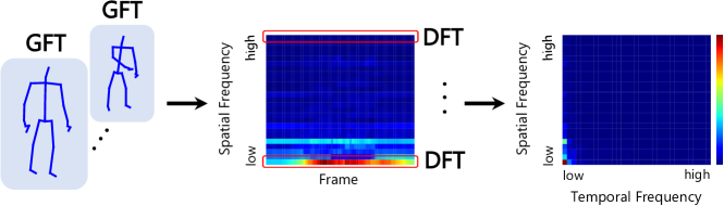
Figure 1: Flow of the joint Fourier transform (JFT) on skeletal sequence data, which encompasses both the graph Fourier transform (GFT) and the discrete Fourier transform (DFT). The GFT is first applied to the skeletal data at each frame, followed by the DFT.

Inspired by these prior efforts, we examine the robustness of skeleton-based action recognition using Fourier analysis. Unlike image classification, where the 2D discrete Fourier transform (DFT) can be used for Fourier analysis, skeleton-based action recognition requires an alternate approach owing to the graph-based representation of the skeletal data. Therefore, we adopt a joint Fourier transform (JFT) [24] that combines the graph Fourier transform (GFT) and DFT, as shown in Fig. 1. By applying the GFT to each frame of the skeletal sequence data and then using the DFT to each graph-frequency component, we analyze the frequencies of the skeletal sequence data along the spatial (graph-frequency) and temporal (time-frequency) directions. This method enables us to explore the difference between CNN-based image classification and GCN-based skeletal action recognition from a Fourier perspective. In experiments with the NTU RGB+D dataset [25], we apply Fourier analysis to compare standard-trained and adversarially-trained GCNs. Our observations reveal that there is no robustness trade-off between adversarial attacks and low-frequency perturbations for GCN-based skeletal action recognition. This finding is interesting because such a trade-off is typically observed in image classification [17, 21]. Furthermore, we explore the robustness against common corruptions, such as Gaussian noise and part occlusion, and find that an experimental result for the case of part occlusion cannot be explained by Fourier analysis alone.

The contributions of this study are as follows.

• A novel application of Fourier analysis is presented to GCN-based skeletal-based action recognition. Specifically, for the first time, we analyze the frequency characteristics of adversarially-trained GCNs against adversarial attacks and common corruptions using the joint Fourier transform.

• Experimental findings indicate that there is no robustness trade-off between adversarial attacks and low-frequency perturbations for skeleton-based action recognition, which is unique in CNN-based image classification.

• Challenges are revealed in comprehensively explaining the robustness of skeleton-based action recognition using Fourier analysis. Specifically, Fourier analysis cannot explain vulnerability against part occlusion corruptions.

The remainder of this paper is organized as follows. Section 2 presents related work on the robustness of skeleton-based action recognition and Fourier analysis approaches in deep learning. Section 3 describes a Fourier analysis method for GCNs. Section 4 presents the experimental results.

2 Related work

This section reviews related work on the robustness of skeleton-based action recognition and the Fourier analysis on robustness of deep models against adversarial attacks and common corruptions.

2.1 Robustness of Skeleton-based Action Recognition

Skeletal motion data offer several advantages over RGB videos, such as robustness to changes in clothing and background and superior computational efficiency [26, 27]. Due to the nature of the skeletal structure, GCNs have been extensively used for skeleton-based action recognition [1, 2, 3, 4, 5, 6].

Recent research has explored adversarial attacks [28, 29] on GCNs for skeleton-based action recognition and revealing the vulnerabilities of GCNs [7, 8, 9, 10]. [10] presented the first white-box adversarial attack on GCNs. Their method perturbs joint locations while preserving temporal coherence, spatial integrity, and anthropomorphic plausibility. [7] proposed a guided manifold walk method to search for adversarial examples in the black-box setting. They also considered the naturalness and imperceptibility of perturbed skeletons. [8] proposed an attack method in both white- and black-box settings and highlighted the importance of considering motion dynamics in analyzing imperceptible adversarial attacks on 3D skeletal motion. [9] indicated that an adversarial attack was possible by only changing the lengths of the bones. All of these studies demonstrate that GCNs are vulnerable to imperceptible adversarial perturbations.

Contrary to these studies on attack, research on defense against adversarial attacks for skeleton-based action recognition remains in its infancy. [14] proposed a Bayesian defense framework based on adversarial training, which is the most effective defense technique against adversarial attacks. Their study demonstrated that adversarial training is effective not only for CNN-based image classification, but also for GCN-based skeletal action recognition. Nevertheless, existing studies on adversarial robustness are limited and not sufficiently comprehensive.

Even so, vulnerability to common corruptions has been explored in several studies. For example, robustness against Gaussian noise [11], part occlusion [12, 13, 15], frame occlusions and jittering noises [13] have been explored. Further investigation into the robustness against both common corruptions and adversarial attacks are essential for enhancing the applicability of deep models in real-world scenarios.

2.2 Fourier analysis of CNN-based image classification

In image classification, recent studies have attempted to explain the robustness of CNNs using frequency analysis [16, 17, 18, 19, 20, 21, 22]. [16] discovered Frequency Principle (F-Principle) that CNNs initially capture dominant low-frequency components before slowly addressing high-frequency ones. [17] demonstrated that standard-trained CNNs predominantly depend on high-frequency components for image classification, while adversarial training encourages CNNs to capture low-frequency components of images. Their further investigation revealed that adversarial training enhances robustness against common high-frequency corruptions, such as Gaussian noise, while degrading robustness against common low-frequency corruptions, such as fog corruption. These findings indicate the existence of a trade-off between robustness against high-frequency and low-frequency perturbations. [19] observed that the frequency characteristics of adversarial robustness may depend on the dataset. [20] investigated the high-frequency biases of standard-trained CNNs. [21] explored these trade-offs by directly changing the frequency profile of the models. [22] identified harmful frequencies for robustness to common corruptions and proposed a method to ignore these harmful frequency components.

[18] explored the relationship between the frequency spectrum of image data and the generalization behavior of CNNs. Their findings emphasized that while CNNs efficiently capture the high-frequency components of images, this capability renders them vulnerable. Conversely, the robustness of CNNs can be enhanced by ignoring high-frequency components. These observations suggest that high-frequency and low-frequency components in images correspond to domain-specific and domain-invariant features, respectively. This insight has subsequently been leveraged in domain generalization [30, 31].

These studies indicate that it is beneficial to use Fourier analysis to understand the robustness of CNNs. However, the frequency analysis of GCN-based skeleton action recognition remains unexplored. Inspired by the Fourier analysis of CNNs by [17], we adapt their methodology to GCNs. This analysis allows us to explore the frequency features captured by GCNs and to assess their robustness across different frequency bands. Furthermore, using the Fourier analysis, we examine the robustness of skeleton-specific common corruptions such as frame loss. These investigations promise to shed light on developing robust GCN models for skeleton-based action recognition.

3 Fourier Analysis for Skeleton-based Action Recognition

Here, we investigate the frequency responses of GCNs for skeleton action recognition to reveal their robustness against adversarial attacks and common corruptions. Rather than using the 2D discrete Fourier transform (DFT), we employ the joint Fourier transform (JFT), which is a frequency analysis tool for time-varying graph signals [24], Furthermore, we use the Fourier heatmap [17] to visualize the sensitivity of deep models in the frequency domain.

3.1 Spatiotemporal Graph for Skeletal Sequence Data

A skeleton sequence for a single person is represented by an undirected graph $G=\quantity(V,E)$, where $V$ is a set of nodes and $E$ is a set of edges. The node set $V$ consists of all $N$ skeleton joints , i.e., $V$ includes $N\times T$ nodes, and the edge set $E$ indicates the intrabody connections of the skeleton. Each node $v_{i}(t)\in V$ is associated with a feature vector of the corresponding joint position $\bm{x}_{i}(t)=(x_{i}(t),y_{i}(t),z_{i}(t))^{\top}\in\mathbb{R}^{3}$ at frame $t$. For example, considering the joint positions themselves, the node feature is $\bm{x}_{i}(t)$. As with other features, joint motion $\bm{v}_{i}(t)=\bm{x}_{i}(t+1)-\bm{x}_{i}(t)$, bone $\bm{b}_{i}(t)=\bm{x}_{i}(t)-\bm{x}_{j}(t)$ ($v_{i}$ and $v_{j}$ is a pair of connected joints), and bone motion $\bm{v}_{i}^{\mathrm{b}}(t)=\bm{b}_{i}(t+1)-\bm{b}_{i}(t)$ have been used  [3, 4, 5]. The set of such feature vectors is represented by

$$\bm{X}=\begin{pmatrix}f_{1}(1)&f_{1}(2)&\ldots f_{1}(T)\\ f_{2}(1)&f_{2}(2)&\ldots f_{2}(T)\\ \vdots&\ddots&\vdots\\ f_{N}(1)&f_{N}(2)&\ldots f_{N}(T)\\ \end{pmatrix}\in\mathbb{R}^{N\times T},$$ (1)

where $f_{i}(t)$ is an $x$, $y$, or $z$ coordinate element of the feature vector associated with $v_{i}(t)$. We omit the dimension of the three-axis channels for simplicity, although the related skeleton sequence is represented by an $N\times T\times 3$ tensor. The skeleton sequence is processed independently for each channel.

To normalize the frame lengths of all skeletal data, linear interpolation along the temporal direction are usually used [4, 5, 6]. We denote the interpolated data for $\bm{X}$ by $I(\bm{X})\in\mathbb{R}^{N\times T^{\prime}}$, where $T^{\prime}$ is set to $64$ in our experiments.

3.2 Standard & Adversarial Training

Let $\mathcal{M}_{\theta}$ be a GCN parameterized by $\theta$. Standard training for $\mathcal{M}_{\theta}$ is performed by solving the following minimization problem

$$\min_{\theta}\mathbb{E}_{\quantity(\bm{X},y)\sim\mathcal{D}}\quantity[\mathcal{L}\quantity(\mathcal{M}_{\theta}\quantity(I(\bm{X}),y))],$$ (2)

where $\mathcal{L}(\cdot)$ is the cross-entropy loss function and $\mathcal{D}$ is an underlying data distribution over pairs of interpolated skeletal data $I(\bm{X})$ and action labels $y$.

Adversarial training in this study is based on the projected gradient descent (PGD) [29], which is a typical and strong attack method. The PGD uses a set of perturbations $S=\{\bm{\delta}\mid\norm{\bm{\delta}}_{p}\leq\epsilon\}$, where $\norm{\bm{\delta}}_{p}$ is the $l_{p}$ norm of $\bm{\delta}\in\mathbb{R}^{T\times N}$ ( we set $p$ as 2) and $\epsilon>0$ denote the supremum of the perturbation norm. Adversarial training for $\mathcal{M}_{\theta}$ with the PGD is performed by solving the following min-max optimization problem [29]

$$\min_{\theta}\mathbb{E}_{\quantity(\bm{X},y)\sim\mathcal{D}}\quantity[\max_{\bm{\delta}_{\mathrm{adv}}\in S}\mathcal{L}\quantity(\mathcal{M}_{\theta}\quantity(I(\bm{X}+\bm{\delta}_{\mathrm{adv}}),y))],$$ (3)

where linear interpolation $I(\cdot)$ is repeatedly applied to adversarially perturbed data $\bm{X}+\bm{\delta}_{\mathrm{adv}}$ in the optimization loop.

3.3 Discrete & Graph Fourier Transforms

DFT and GFT form the basis for the JFT on spatiotemporal graph $G$, as is discussed in the following subsection. Additionally, DFT and GFT are used to generate low-frequency or high-frequency Gaussian noise signals, which are used to validate the trade-off in robustness against low-frequency and high-frequency corruptions, as discussed in Section 4.2.3.

We let the GFT be defined first. The GFT on $\bm{X}$ is defined by

$$\text{GFT}\quantity(\bm{X})=\bm{U}^{\top}\bm{X},$$ (4)

where $\bm{U}\in\mathbb{R}^{N\times N}$ is the eigenvector matrix of the Laplacian matrix $\bm{L}$ of the spatial subgraph of $G$. The Laplacian matrix is defined by $\bm{L}=\bm{D}-\bm{A}\in\mathbb{R}^{N\times N}$, where $\bm{A}$ and $\bm{D}$ denote the adjacency and degree matrices of the spatial skeletal structure, respectively. Let $\lambda_{k}\in\mathbb{R}$ and $\bm{u}_{k}\in\mathbb{R}^{N}$ be the $k$-th eigenvalue and eigenvector of $\bm{L}$. The eigenvector matrix $\bm{U}$ is obtained by applying the eigen-decomposition to $\bm{L}$ as follows

$$\bm{L}=\bm{U}\bm{\Sigma}\bm{U}^{\top},$$ (5)

where $\bm{U}=\quantity[\bm{u}_{1},\ldots,\bm{u}_{N}]$ and $\bm{\Sigma}=\mathrm{diag}\quantity(\lambda_{1},\ldots,\lambda_{N})$. Here, the eigenvalues are sorted as $\lambda_{1}\geq\lambda_{2}\geq\cdots>\lambda_{N}=0$, where the larger the eigenvalue is, the higher the frequency.

The DFT on $\bm{X}$ is defined by

$$\text{DFT}\quantity(\bm{X})=\bm{X}\bm{W},$$ (6)

where $\bm{W}\in\mathbb{R}^{T\times T}$ is the DFT matrix, defined by

$$\bm{W}=\begin{pmatrix}1&1&1&\ldots&1\\ 1&\omega&\omega^{2}&\ldots&\omega^{T-1}\\ 1&\omega^{2}&\omega^{4}&\ldots&\omega^{2(T-1)}\\ \vdots&\vdots&\vdots&\ddots&\vdots\\ 1&\omega^{T-1}&\omega^{2(T-1)}&\ldots&\omega^{(T-1)(T-1)}\\ \end{pmatrix},$$ (7)

where $\omega=e^{-2\pi j/T}$ and $j^{2}=-1$.

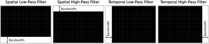
Figure 2: Spatial low-pass (leftmost) and high-pass (left second) filtering are performed by masking the Fourier spectrum along the spatial frequency axis. Temporal low-pass (right second) and high-pass (rightmost) are performed by masking the Fourier spectrum along the temporal frequency axis.

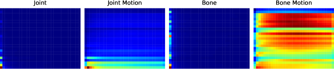
Figure 3: Average Fourier spectrum over all tests skeleton data for joint, joint motion, bone, and bone motion features. The vertical and horizontal axes represent spatial and temporal frequency, respectively. From these figures, for example, we can see the Fourier spectrum of the joint feature (leftmost) is concentrated at low frequencies in the spatiotemporal frequency domain.

We generate low-frequency or high-frequency Gaussian noises that is added to skeletal data $\bm{X}$ using the GFT and DFT. Let $\bm{V}$ be the Gaussian white noise on $\mathbb{R}^{N\times T}$, where each element of $\bm{V}$ is independently sampled from a zero-mean Gaussian distribution $\mathcal{N}(0,\sigma^{2})$. Spatial filtering or graph spectral filtering on $\bm{V}$ is defined by

$$\widetilde{\bm{V}_{\mathrm{s}}}=\bm{M}_{\mathrm{s}}\text{GFT}(\bm{V}),$$ (8)

where $\widetilde{\bm{V}_{\mathrm{s}}}$ is the filtering output in the spatial frequency domain and $\bm{M}_{\mathrm{s}}=\mathrm{diag}(m_{\mathrm{s},1},m_{\mathrm{s},2},\ldots,m_{\mathrm{s},N})$ is the $N\times N$ binary diagonal matrix for spatial filtering. For instance, if $\bm{M}_{\mathrm{s}}=\mathrm{diag}(0,0,\ldots,0,1,1)$, as shown in Fig. 2 (leftmost), a low-frequency Gaussian noise with a bandwidth of 2 is generated by applying the inverse GFT to $\widetilde{\bm{V}_{\mathrm{s}}}$. If $\bm{M}_{\mathrm{s}}=\mathrm{diag}(1,1,0,\ldots,0)$, as shown in Fig. 2 (left second), High-frequency Gaussian noise with a bandwidth of 2 is generated. Similarly, temporal filtering on $\bm{V}$ is defined by

$$\widetilde{\bm{V}_{\mathrm{t}}}=\text{DFT}(\bm{V})\bm{M}_{\mathrm{t}},$$ (9)

where $\widetilde{\bm{V}_{\mathrm{t}}}$ is the filtering output in the temporal frequency domain and $\bm{M}_{\mathrm{t}}=\mathrm{diag}(m_{\mathrm{t},1},m_{\mathrm{t},2},\ldots,m_{\mathrm{t},T})$ is the $T\times T$ binary diagonal matrix for temporal filtering. Similar to the GFT, $\bm{M}_{\mathrm{t}}=\mathrm{diag}(0,0,\ldots,0,1,1)$ and $\bm{M}_{\mathrm{t}}=\mathrm{diag}(1,1,0,\ldots,0)$ generate low-frequency and high-frequency Gaussian noises with a bandwidth of 2, as shown in Fig. 2 (right second) and (rightmost), respectively.

3.4 Joint Fourier Transform and Fourier Heatmap

We adopt the JFT [24] for Fourier analysis on spatiotemporal graph G, which encompasses both the GFT and DFT. Initially, the GFT is implemented on the spatial subgraph of $G$ for each frame to extract spatial frequency characteristics, followed by the application of the DFT to extract temporal frequency characteristics of $G$, as shown in Fig. 1.

The JFT on $\bm{X}$ is defined by combining the GFT and DFT as follows:

$$\text{JFT}\quantity(\bm{X})=\bm{U}^{\top}\bm{X}\bm{W}.$$ (10)

For Fourier analysis on skeletal data, we compute the average spectrum over all test data of $\bm{X}$ using the JFT, and visualize these values using the heatmaps shown in Fig. 3, where the horizontal and vertical axes represent temporal and spatial frequencies, respectively.

Additionally, we employ Fourier heatmaps [17] to visualize the sensitivity of the GCNs for specific frequency signals. A signal of spatial frequency $\lambda_{k}$ (the $k$-th eigenvalue of $\bm{L}$) and temporal frequency $l/T$, denoted by $\bm{F}_{k,l}\in\mathbb{R}^{N\times T}$, is generated by setting the JFT of $\bm{F}_{k,l}$ to

$$\text{JFT}(\bm{F}_{k,l})=\bordermatrix{&&&&l^{\text{th}}&&&\cr&0&&0&0&0&\ldots&0\cr&\vdots&\vdots&\vdots&\vdots&\vdots&\vdots&\vdots\cr k^{\text{th}}&0&\ldots&0&1&0&\ldots&0\cr&\vdots&\vdots&\vdots&\vdots&\vdots&\vdots&\vdots\cr&0&\ldots&0&0&0&\ldots&0\cr},$$ (11)

where the right-hand side matrix takes $1$ for only the $(k,l)$-element and $0$ otherwise. Using $\bm{F}_{k,l}$, a perturbed signal of a skeleton sequence $\bm{X}$ is generated by

$$\bm{X}^{\prime}=I(\bm{X})+rv\bm{F}_{k,l},$$ (12)

where $r$ is sampled uniformly at random from $\quantity{-1,1}$, $v>0$ is the norm of the perturbation, and $\bm{F}_{k,l}$ is supposed to be normalized as $||\bm{F}_{k,l}||_{2}=1$. The Fourier heatmap is generated by plotting the average error rate of 1000 randomly sampled test data for every frequency $k=1,2,\ldots,N$ and $l=1,2,\ldots,T$. The closer to red a region of the Fourier heatmap is, the more sensitive the GCNs at the corresponding frequency. In other words, to recognize human actions, GCNs capture skeletal signals that contain such sensitive frequencies. The high sensitivity brings vulnerability to the GCNs.

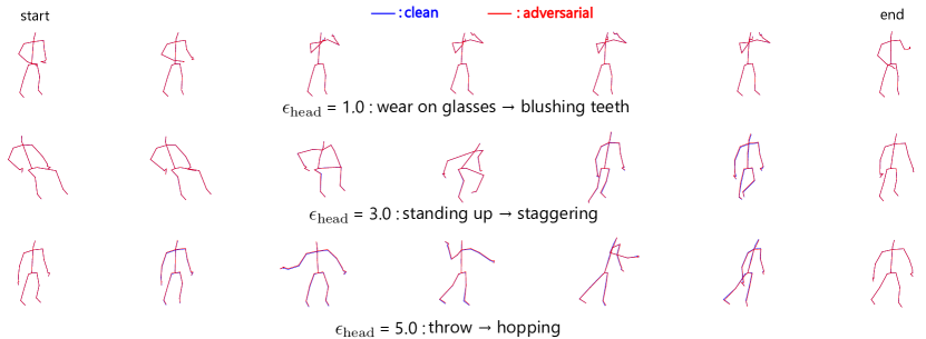
Figure 4: Adversarial examples generated by the $l_{2}$-PGD. Clean (blue) and adversarial (red) examples are superimposed for three example actions. These two almost overlap and are highly imperceptible. For each action, action labels before and after adversarial attacks are provided.

4 Experiment

Using frequency analysis, we conduct a comparative analysis of the robustness for the standard-trained and adversarially-trained GCNs. First, we investigate the robustness and vulnerability in the frequency domain using Fourier heatmaps. The visualization provides basic insights into the robustness of adversarial training. Next, we analyze the spectral distributions of adversarial perturbations to the GCNs. This analysis reveals the frequency characteristics of adversarial attacks. Furthermore, we explore whether the robustness trade-off that has been established in CNN-based image classification exists similarly in GCN-based skeletal action recognition. Finally, we evaluate the robustness of the GCNs against common corruptions.

4.1 Experimental Setting

4.1.1 Dataset

We conduct our experiments on NTU RGB+D [25], which contains 56,880 skeletal data with 60 action classes. We divide the whole data into training and test data according to the subjects (cross-subject setting). The training and test datasets comprise 40,320 and 16,560 samples, respectively. For the validation data, we randomly sample 5% from the training data.

4.1.2 Model

We chose ST-GCN [1] as a baseline GCN and TCA-GCN [5] as one of the state-of-the-art GCNs. We have not assessed robust models, as it is challenging to distinguish between GCN’s inherent robustness and potential vulnerabilities against adversarial attacks and common corruptions. Our primary focus is on evaluating the pure robustness of GCN-based action recognition. A comprehensive validation against robust models will be addressed in future work.

We train ST-GCN and TCA-GCN for joint $\bm{x}_{i}(t)$, joint motion $\bm{v}_{i}(t)$, bone $\bm{b}_{i}(t)$, and bone motion $\bm{v}_{i}^{\mathrm{b}}(t)$, respectively, using official codes provided by those authors. To guarantee convergence in training, we execute at least 80 epochs for the ST-GCN and 75 epochs for the TCA-GCN and adopt early stopping with patience 20 for both models. For the other hyperparameters, we use the same ones of the official codes.

Table 1: Comparison of clean accuracy between standard-trained (ST) and adversarially-trained (AT) models.

Model	Joint	Joint Motion	Bone	Bone Motion
ST-GCN (ST)	85.3%	84.8%	85.4%	84.4%
ST-GCN (AT)	79.8%	73.1%	79.7%	76.0%
TCA-GCN (ST)	89.4%	86.7%	89.2%	86.3%
TCA-GCN (AT)	82.1%	77.2%	82.2%	78.4%

Table 2: Comparison of adversarial accuracy between standard-trained (ST) and adversarially-trained (AT) models.

Model	$\epsilon_{\mathrm{head}}=1$	$\epsilon_{\mathrm{head}}=3$	$\epsilon_{\mathrm{head}}=5$
ST-GCN ST (Joint)	26.3%	6.00%	1.63%
ST-GCN AT (Joint)	74.6%	61.2%	47.7%
TCA-GCN ST (Joint)	16.7%	1.72%	0.19%
TCA-GCN AT (Joint)	76.8%	64.6%	52.4%
ST-GCN ST (Joint Motion)	9.30%	0.61%	0.06%
ST-GCN AT (Joint Motion)	64.2%	48.3%	35.8%
TCA-GCN ST (Joint Motion)	2.84%	0.04%	0.00%
TCA-GCN AT (Joint Motion)	69.0%	51.6%	36.5%
ST-GCN ST (Bone)	8.99%	0.35%	0.07%
ST-GCN AT (Bone)	71.5%	52.5%	32.9%
TCA-GCN ST (Bone)	8.35%	0.21%	0.01%
TCA-GCN AT (Bone)	76.1%	60.8%	44.5%
ST-GCN ST (Bone Motion)	0.87%	0.02%	0.00%
ST-GCN AT (Bone Motion)	62.2%	40.5%	24.5%
TCA-GCN ST (Bone Motion)	0.39%	0.03%	0.02%
TCA-GCN AT (Bone Motion)	61.3%	46.5%	31.8%

4.1.3 Adversarial Attack

To evaluate adversarial robustness, we use the $l_{2}$-PGD attack rather than skeleton-specific attacks such as SMART [8] and BASAR [7]. These skeleton-specific attacks are designed to be imperceptible by imposing additional constraints such as fixing bone length. These constraints complicate the direct control of the attack strength. In contrast, the PGD attack strength can be simply controlled by increasing a perturbation threshold $\epsilon$. Therefore, using the PGD attack, we can systematically assess the robustness of GCNs. Furthermore, we can compare GCN-based action recognition with CNN-based image classification, because the PGD attack is commonly used for CNNs (e.g., as seen in [17]).

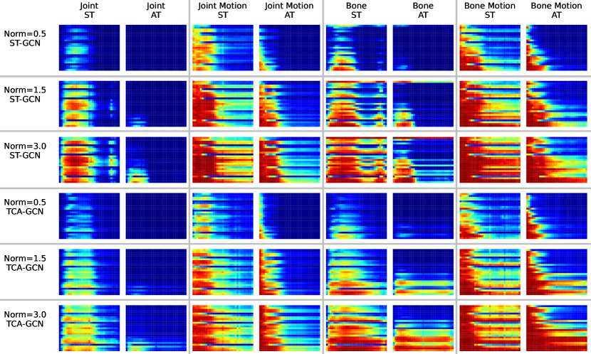
Figure 5: Fourier heatmaps of standard-trained (ST) and adversarially-trained (AT) GCNs. The top and bottom three rows display those of the ST-GCNs and TCA-GCNs, respectively, for each of the four features (joint, joint motion, bone, bone motion) and three perturbation norms $v\in\{0.5,1.5,3.0\}$.

To normalize the attack strength to each piece of skeletal data, we set the perturbation threshold $\epsilon$ as $\epsilon=l_{\mathrm{head}}\times\epsilon_{\mathrm{head}}$, where $l_{\mathrm{head}}$ is the head length of each skeletal datum. Fig. 4 displays adversarial examples when $\epsilon_{\mathrm{head}}=1.0,3.0,5.0$. We do not impose any naturalness constraints on the attacker, except for the perturbation norm. Nevertheless, we observe that adversarial attacks are highly imperceptible because linear interpolation in Section 3.1 suppresses large jittering.

4.1.4 Adversarial Training

Adversarial training [29] is an effective method for defending against adversarial attacks. We use Free [32] for adversarial training due to its computational efficiency. For Free, the number of hop steps is set to four, and the threshold is set to $\epsilon_{\mathrm{head}}=3$. Table 1 shows the accuracies of standard-trained and adversarially-trained models. As is well established, adversarial training performs less effectively than standard training for clean data. To verify that adversarial training enhances adversarial robustness, we conduct preliminary experiments on robustness of the standard-trained and adversarially-trained models with thresholds $\epsilon_{\mathrm{head}}\in\quantity{1.0,3.0,5.0}$ and 10 iterations. Then, we attack each model by perturbing clean data correctly classified by both models to take the difference in clean accuracy into consideration. In Table 2, we can see that adversarial training demonstrates higher adversarial robustness than standard training.

4.1.5 Evaluation Metric

As shown in Table 1, there is a difference in clean accuracy between standard-trained and adversarially-trained models. For a fair comparison of robustness, we remove a such difference. More specifically, when we evaluate the robustness, we perturb clean data correctly classified by both models and use accuracy for these perturbed data as an evaluation metric.

4.2 Results

4.2.1 Frequency Analysis of Adversarial Training

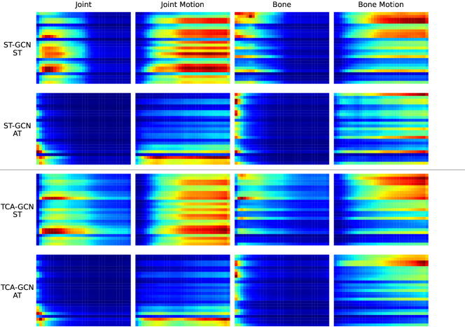
Figure 6: Average Fourier spectrum of adversarial perturbations in the spatiotemporal frequency domain. The heatmaps plot the estimation of $\mathbb{E}\quantity[|\mathrm{JFT}(I(\bm{X}+\bm{\delta}_{\mathrm{adv}})-I(\bm{X}))|]$, where $\bm{X}$ is the clean data and the expectation is chosen over the adversarial examples that successfully attack each model.

The Fourier heatmap examines the frequency characteristics of standard and adversarial training. Fig. 5 shows Fourier heatmaps plot the average error rates of 1000 randomly sampled test data points for every frequency. The top and bottom three rows display the Fourier heatmaps of the ST-GCNs and TCA-GCNs, respectively, for each of the four features (joint, joint motion, bone, bone motion) in Section 3.1 and three perturbation norms $v\in\{0.5,1.5,3.0\}$ in Eq. (12).

Fig. 5 reveals the following frequency characteristics. The standard-trained models are sensitive to temporal low-frequency perturbations (i.e., the left half of the maps). In other words, the models do not capture high-frequency signals in time, whereas they do capture signals from low to high frequencies in space. The adversarially-trained models become more insensitive, especially for high-frequency perturbations (i.e., the upper right of the maps), resulting in robustness to high-frequency perturbations. Joint motion and bone motion features introduce more vulnerability against high-frequency perturbations than the joint and bone features, respectively. This vulnerability is reasonably attributed to motion (differential) features generally being more sensitive to high-frequency perturbations than positional features. These frequency characteristics do not depend on the network architecture, and the two GCNs have similar characteristics.

Table 3: List of scaled norms for spatially or temporally filtered Gaussian noises.

Filter	Joint	Joint Motion	Bone	Bone Motion
Spatial Low	17.0	3.50	6.40	1.10
Spatial High	77.0	20.0	5.90	4.80
Temporal Low	31.0	2.0	9.90	0.60
Temporal High	77.0	19.0	24.0	14.0

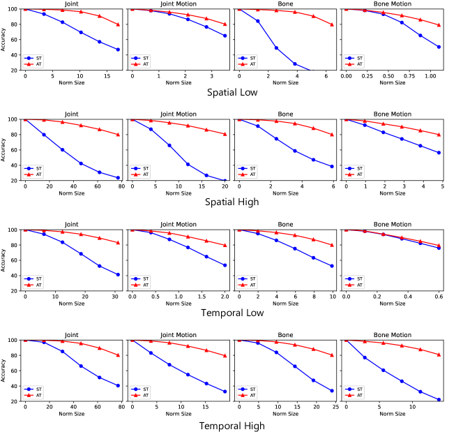
Figure 7: Accuracy comparison of standard-trained (blue) and adversarially-trained (red) GCNs for changes in the Gaussian noise norm with a fixed bandwidth of 2: (top) spatial low-pass filter, (second) spatial high-pass filter, (third) temporal low-pass filter, and (bottom) temporal high-pass filter.

These results prove that adversarial training can improve the robustness in the higher frequencies, and the improvement is also observable in CNN-based image classification [17, 18, 20]. In contrast, the lower frequency characteristics of the CNNs and GCNs are slightly different. In CNN-based image classification, adversarial training sacrifices the robustness of the standard-trained models in the lowest frequencies (i.e., the lower left of the maps), whereas this is not always the case in GCN-based action recognition. For example, the adversarially-trained models learned with the joint and bone features do not become more vulnerable than the standard-trained models at the lowest frequencies.

4.2.2 Frequency Analysis of Adversarial Attack

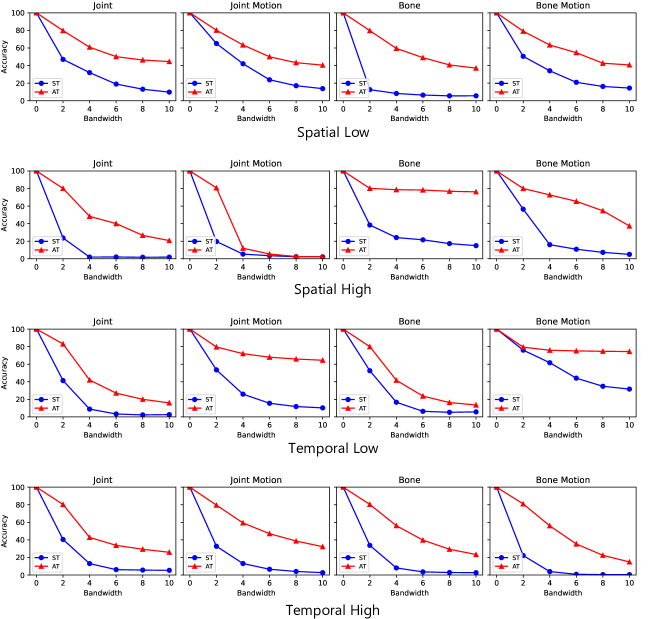
Figure 8: Accuracy comparison of standard-trained (blue) and adversarially-trained (red) GCNs for changes in the Gaussian noise bandwidth with the scaled norm in Table. 3. (top) spatial low-pass filter, (second) spatial high-pass filter, (third) temporal low-pass filter, and (bottom) temporal high-pass filter.

The frequency characteristics of adversarial attacks are examined using the spectral distribution of successful adversarial attacks. Fig. 6 shows the spectral distributions, which are obtained by estimating the average amplitude of successful adversarial examples, i.e., $\mathbb{E}\quantity[|\mathrm{JFT}(I(\bm{X}+\bm{\delta}_{\mathrm{adv}})-I(\bm{X}))|]$, where $\bm{X}$ is clean skeletal data and $\bm{\delta}_{\mathrm{adv}}$ is an adversarial perturbation that successfully attacks a given GCN. Here, $I(\cdot)$ is the linear interpolation operation in Section 3.1.

Fig. 6 shows that the spectral distributions of the adversarial attacks on the standard-trained models are broadly distributed, whereas those on the adversarially-trained models are concentrated in the lower frequencies. These frequency characteristics indicate that the adversarially-trained models capture the features from the lower frequency signals better than the standard-trained models. This observation supports the hypothesis that adversarial training provides robustness against high-frequency perturbations, as discussed in the previous subsection. However, the adversarially-trained models with the bone motion feature remain vulnerable in the high-frequency domain (i.e., the rightmost column in Fig. 6). This phenomenon reasonably leads us to conclude that the bone feature contains high-frequency signals [20] as shown in Fig. 3 (i.e., the rightmost column).

4.2.3 Robustness Trade-off between High-Frequency and Low-Frequency Perturbations

We examine whether a trade-off exists where adversarially-trained models are robust to high-frequency perturbations but highly vulnerable to low-frequency perturbations. This examination is motivated by the existence of the same trade-off as found in CNN-based image classification [17, 21]. The trade-off is evaluated by adding low- or high-frequency Gaussian noise, as described in Section 3.3, to the clean data that both models correctly classify. The norm of the Gaussian noise is adjusted such that the accuracy of either the standard-trained model or the adversarially-trained model is approximately 80%. This adjustment is required for a fair comparison because the appropriate norm differs between the four features. These norms are listed in Table 3 and denoted as scaled norms. In the following experiments, we use the ST-GCN because there is no significant difference in the frequency characteristics of the two architectures.

Table 4: List of scaled norms for spatiotemporally filtered Gaussian noises.

Filter	Joint	Joint Motion	Bone	Bone Motion
Spatial & Temporal Low	78.0	5.60	22.0	1.25
Spatial & Temporal High	355	220	35.0	130

First, we evaluate the accuracies of the standard-trained model (blue) and the adversarially-trained model (red), as shown in Fig. 7, for changes in the Gaussian noise norm while maintaining a fixed bandwidth of 2. The norm is changed at 20%, 40%, 60%, 80%, and 100% of the scaled norm. The top two and bottom two rows in Fig. 7 show the accuracies when perturbed with spatially or temporally filtered Gaussian noises, respectively. In all cases, the adversarially-trained model (red) is more robust than the standard-trained model (blue).

Next, we evaluate the accuracies of the two models upon changing the Gaussian noise bandwidth while keeping the norm fixed at the scaled norm. The results are shown in Fig. 8 and indicate that the adversarially-trained model (red) is also more robust than the standard model. Finally, we evaluate the accuracies for changes in the spatially and temporally filtered Gaussian noise norm while keeping the norm fixed. Table 4 lists the scaled norm for the experiment, and Fig.  9 also proves that the adversarially-trained model (red) is again more robust.

In summary, these results indicate that GCN-based skeletal action recognition does not suffer from the same robustness trade-offs as CNNs. In some exceptions, the accuracy of the adversarially-trained and standard-trained models are comparable, e.g., the bone motion feature labeled "Temporal Low" in Fig. 7. These results arise because the robustness of the two GCNs does not differ significantly within that frequency band, as evident from the corresponding frequency band of the Fourier heatmap in Fig. 5. Except for such frequency bands, adversarial training can improve the GCNs robustness to both low- and high-frequency perturbations, i.e., without sacrificing robustness in the low-frequency domain.

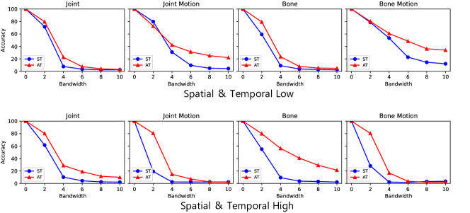
Figure 9: Accuracy comparison of standard-trained (blue) and adversarially-trained (red) GCNs for changes in the Gaussian noise bandwidth with the scaled norm in Table 4: (top) spatiotemporal low-pass filter, (bottom) spatiotemporal high-pass filter.

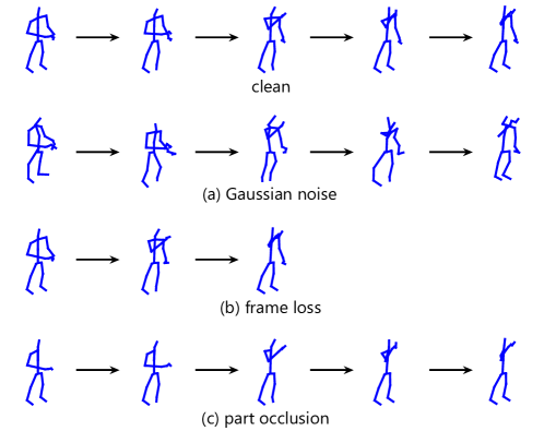
Figure 10: Examples of common corruptions in skeleton-based action recognition: (a) Gaussian noise, (b) frame loss, and (c) part occlusion.

4.2.4 Robustness to Common Corruptions

We evaluate the robustness to common corruptions. In image classification, common corruptions to image data include high-frequency corruptions, such as Gaussian noise and shot noise, and low-frequency corruptions, such as motion blur and fog [33]. The trade-off between accuracy and adversarial robustness makes CNN-based image classifiers robust to high-frequency corruptions but vulnerable to low-frequency corruptions. However, the experiment in the previous section demonstrates that such a trade-off does not exist for the GCNs. Therefore, adversarial training is expected to be more robust to common corruptions than standard training, regardless of its frequency spectra. We experimentally examine this conclusion based on the following three common corruptions for skeleton data, as shown in Fig. 10.

• Gaussian noise: the skeletal data are perturbed by adding a zero-mean Gaussian noise with standard deviation $\sigma=0.01,0.03,0.05$.

• Frame loss: Each frame of the skeletal sequence data is randomly lost. Loss rate $p$ is a uniform random number in the $[0,1]$ interval. The frame length is adjusted when input to the GCNs by linearly interpolating the lost frames.

• Part occlusion [12]: a part of the skeletal data is occluded. The skeletal data are divided into five parts: left arm (part 1), right arm (part 2), both hands (part 3), both legs (part 4), and torso (part 5), and either part coordinates are set to 0.

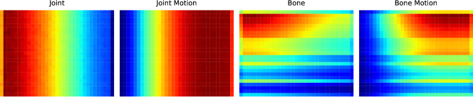
Figure 11: Average Fourier spectrum of Gaussian noise corruptions with standard deviation $\sigma=0.05$ in the spatiotemporal frequency domain.

To provide a Fourier analysis of the common corruptions, we compute their spectral distributions as shown in Figs. 11–13. These distributions are given by $\mathbb{E}\quantity[|\mathrm{JFT}(I(C(\bm{X}))-I(\bm{X}))|]$, where $\bm{X}$ is clean skeletal data and $C(\cdot)$ is one of the three corruptions.

Table 5: Comparison of accuracy against Gaussian noise corruptions with standard deviation $\sigma$ for standard-trained (ST) and adversarially-trained (AT) models.

	$\sigma=0.01$	$\sigma=0.03$	$\sigma=0.05$
ST-GCN ST (Joint)	94.3%	67.4%	42.5%
ST-GCN AT (Joint)	99.8%	99.5%	98.8%
TCA-GCN ST (Joint)	95.4%	82.7%	59.8%
TCA-GCN AT (Joint)	99.9%	99.0%	96.8%
ST-GCN ST (Joint Motion)	74.4%	34.1%	19.1%
ST-GCN AT (Joint Motion)	98.7%	87.9%	64.9%
TCA-GCN ST (Joint Motion)	74.8%	40.2%	20.7%
TCA-GCN AT (Joint Motion)	99.2%	87.6%	65.7%
ST-GCN ST (Bone)	87.7%	25.6%	10.9%
ST-GCN AT (Bone)	99.8%	99.0%	97.1%
TCA-GCN ST (Bone)	91.7%	50.7%	20.1%
TCA-GCN AT (Bone)	99.6%	97.4%	90.6%
ST-GCN ST (Bone Motion)	43.5%	6.2%	1.28%
ST-GCN AT (Bone Motion)	98.1%	84.0%	56.5%
TCA-GCN ST (Bone Motion)	59.6%	13.1%	2.7%
TCA-GCN AT (Bone Motion)	95.8%	88.7%	71.9%

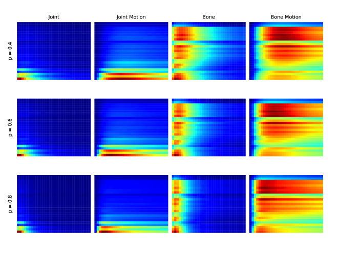
Figure 12: Average Fourier spectrum of frame loss corruptions with loss rates $p=0.4,0.6,0.8$ in the spatiotemporal frequency domain.

Table 6: Comparison of accuracy against frame loss corruptions with loss rate $p$ for standard-trained (ST) and adversarially-trained (AT) models.

	$p=0.4$	$p=0.6$	$p=0.8$
ST-GCN ST (Joint)	97.3%	94.8%	84.4%
ST-GCN AT (Joint)	97.4%	95.3%	88.8%
TCA-GCN ST (Joint)	96.2%	90.5%	80.6%
TCA-GCN AT (Joint)	97.7%	96.2%	91.1%
ST-GCN ST (Joint Motion)	92.6%	78.8%	55.3%
ST-GCN AT (Joint Motion)	94.9%	90.9%	77.9%
TCA-GCN ST (Joint Motion)	92.9%	81.0%	61.3%
TCA-GCN AT (Joint Motion)	95.5%	91.4%	80.3%
ST-GCN ST (Bone)	97.6%	95.9%	86.7%
ST-GCN AT (Bone)	97.5%	95.4%	89.2%
TCA-GCN ST (Bone)	96.1%	89.1%	78.3%
TCA-GCN AT (Bone)	97.7%	95.6%	90.7%
ST-GCN ST (Bone Motion)	93.1%	81.3%	55.7%
ST-GCN AT (Bone Motion)	95.9%	92.3%	80.1%
TCA-GCN ST (Bone Motion)	92.7%	79.7%	59.6%
TCA-GCN AT (Bone Motion)	87.9%	77.9%	68.8%

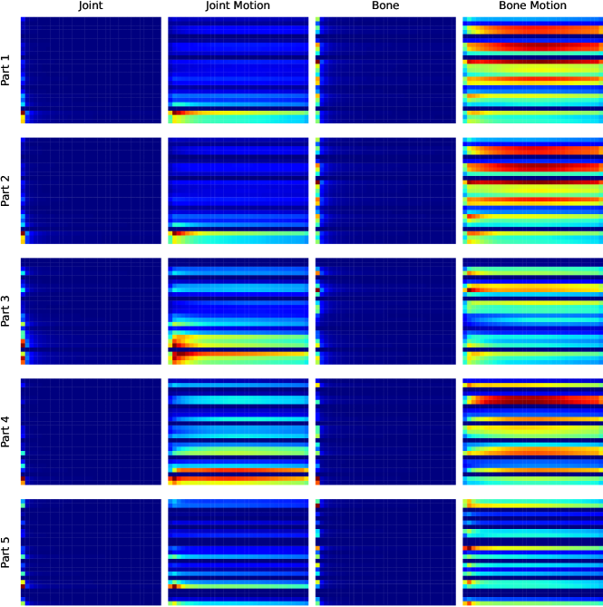
Figure 13: Spectral distributions of part occlusion corruptions in the spatiotemporal frequency domain.

Table 7: Comparison of accuracy against part occlusion corruptions for standard-trained (ST) and adversarially-trained (AT) models.

	part 1	part 2	part 3	part 4	part 5
ST-GCN ST (Joint)	86.7%	72.8%	80.5%	95.5%	69.3%
ST-GCN AT (Joint)	78.3%	61.3%	48.5%	87.5%	63.6%
TCA-GCN ST (Joint)	84.8%	69.6%	61.8%	90.4%	79.4%
TCA-GCN AT (Joint)	73.6%	58.5%	47.7%	72.8%	74.8%
ST-GCN ST (Joint Motion)	83.2%	67.2%	95.8%	92.0%	74.1%
ST-GCN AT (Joint Motion)	75.0%	57.6%	62.0%	88.2%	89.4%
TCA-GCN ST (Joint Motion)	83.5%	71.2%	84.1%	85.0%	82.7%
TCA-GCN AT (Joint Motion)	73.5%	56.6%	68.4%	87.0%	93.2%
ST-GCN ST (Bone)	82.0%	63.8%	49.4%	59.7%	46.9%
ST-GCN AT (Bone)	65.0%	52.0%	62.6%	75.0%	54.7%
TCA-GCN ST (Bone)	83.8%	66.0%	33.9%	67.6%	57.6%
TCA-GCN AT (Bone)	71.4%	52.3%	39.4%	62.9%	60.2%
ST-GCN ST (Bone Motion)	84.4%	67.9%	85.7%	88.9%	73.3%
ST-GCN AT (Bone Motion)	73.6%	56.8%	71.1%	87.0%	83.8%
TCA-GCN ST (Bone Motion)	84.8%	70.6%	85.8%	81.4%	83.6%
TCA-GCN AT (Bone Motion)	73.2%	54.3%	58.3%	85.2%	81.7%

Gaussian Noise

Fig. 11 shows the average Fourier spectrum distributions for the four features, and Table 5 lists the accuracies of the standard-trained and adversarially-trained two GCNs with standard deviation $\sigma=0.01,0.03,0.05$. As depicted in Fig. 11, the frequency characteristics of Gaussian noise corruption differ for the four features. For example, the joint feature largely includes temporal low-frequency signals (i.e., the left half of the map), whereas the joint motion feature includes temporal high-frequency signals (i.e., the right half of the map).

For such corruptions, we predict which frequency bands are vulnerable from the Fourier heatmap in Fig. 5. For example, the Fourier heatmap of the joint feature, as shown in Fig. 5 (i.e., leftmost column) indicates that the standard-trained models are vulnerable in the temporal low-frequency domain, but the adversarially-trained models are more robust in all frequency domains. Therefore, adversarially-trained models are expected to provide better accuracies in all cases. Table 5 supports this prediction. The same holds for the other three features. Hence, adversarial training yields robustness to Gaussian noise corruptions for GCN-based skeletal action recognition.

Frame Loss

Fig. 12 shows the average Fourier spectra of the frame loss corruptions for the four features, and Table 6 lists the accuracies of the standard-trained and adversarially-trained two GCNs with frame loss rate $p=0.4,0.6,0.8$. Table 6 shows that the adversarially-trained models achieve higher or comparable accuracy to the standard-trained models in most cases. The exception is the case of the TCA-GCN bone motion feature (bottom row of Table 6), where the standard-trained TCA-GCN provides better performance in accuracy at loss rates $p=0.4$ and $0.6$. This reversal is attributed to the fact that the frame losses at p=0.4 and 0.6 contain more frequencies in the spatial low-frequency and the temporal mid- to high-frequency bands, as shown in Fig. 12. In these frequency bands, the Fourier heatmap in Fig. 5 shows that the standard-trained TCA-GCN is more robust for the bone motion features. Except for such frequency bands, the adversarially-trained models are more robust over a wider frequency range than the standard-trained models, as with Gaussian corruption.

Part Occlusion

Finally, we examine the robustness against part occlusion corruptions. Fig. 13 shows the average Fourier spectrum distributions, and Table 7 lists the accuracies for each type of model. In contrast to the other corruptions, Table 7 indicates that the standard-trained models are more robust in most cases. In other words, these corruptions cannot be explained using the Fourier heatmaps. For example, the spectrum for the bone motion feature of part 1 (i.e., the top right in Fig. 13) includes high-frequency spatial signals, and therefore the adversarially-trained models should be more robust to the corruption. However, the results in Table 7 demonstrate that the standard-trained models are more robust to this scenario. A possible alternative explanation is that the part occlusion corruptions cause a portion of the skeletal signals to be missing, resulting in the loss of the features necessary for action recognition. The missing signal problem cannot be explained from the Fourier perspective, and other approaches need to be considered.

5 Conclusions

This study examines the robustness of the GCNs for skeleton-based action recognition against adversarial attacks and common corruptions. Fourier analysis of the robustness of GCNs is reported. We compute the average Fourier spectra of adversarial perturbations and common corruptions using the JFT, which is a combination of the GFT and DFT. Furthermore, the frequency effects of both standard and adversarial training are explored using the Fourier heatmap.

Our experiments reveal that the standard-trained models are sensitive to high-frequency perturbations, and adversarial training suppresses this sensitivity and enhances robustness to high-frequency perturbations. This robustness against high frequencies is also known in CNN-based image classification. Our interesting finding is that the GCNs for skeleton-based action recognition do not suffer from a robustness trade-off between adversarial robustness and low-frequency perturbations (as do CNNs). While the absence of the trade-off remains an open problem, our experiments lead to the following observations. As depicted in Fig. 3, all four skeletal features display distinct frequency characteristics, yet no trade-off is observed. This is true even for the joint feature, which exhibits a low-frequency concentration similar to natural images. Thus, our experimental results suggest that the discrepancy in robustness primarily stems from the inherent differences between CNNs and GCNs, rather than the frequency characteristics of the skeletal features. It will be necessary to explore this difference not only through Fourier analysis but also through other analysis methods and perspectives. Furthermore, given the transition from CNNs and GCNs to Transformer architectures in computer vision, frequency analysis of Transformers, as in [34], will be important research for robust computer vision.

References

- [1] Sijie Yan, Yuanjun Xiong, and Dahua Lin. Spatial temporal graph convolutional networks for skeleton-based action recognition. In AAAI Conference on Artificial Intelligence, volume 34, pages 7444–7452, 2018.
- [2] Pengfei Zhang, Cuiling Lan, Wenjun Zeng, Junliang Xing, Jianru Xue, and Nanning Zheng. Semantics-guided neural networks for efficient skeleton-based human action recognition. In Conference on Computer Vision and Pattern Recognition (CVPR), pages 1109–1118, 2020.
- [3] Ke Cheng, Yifan Zhang, Xiangyu He, Weihan Chen, Jian Cheng, and Hanqing Lu. Skeleton-based action recognition with shift graph convolutional network. In Conference on Computer Vision and Pattern Recognition (CVPR), pages 180–189, 2020.
- [4] Yuxin Chen, Ziqi Zhang, Chunfeng Yuan, Bing Li, Ying Deng, and Weiming Hu. Channel-wise topology refinement graph convolution for skeleton-based action recognition. In International Conference on Computer Vision (ICCV), pages 13339–13348, 2021.
- [5] Shengqin Wang, Yongji Zhang, Minghao Zhao, Hong Qi, Kai Wang, Fenglin Wei, and Yu Jiang. Skeleton-based action recognition via temporal-channel aggregation. arXiv:2205.15936, 2022.
- [6] Jungho Lee, Minhyeok Lee, Dogyoon Lee, and Sangyoun Lee. Hierarchically decomposed graph convolutional networks for skeleton-based action recognition. In International Conference on Computer Vision (ICCV), pages 10444–10453, October 2023.
- [7] Yunfeng Diao, Tianjia Shao, Yong-Liang Yang, Kun Zhou, and He Wang. Basar:black-box attack on skeletal action recognition. In Conference on Computer Vision and Pattern Recognition (CVPR), pages 7593–7603, 2021.
- [8] He Wang, Feixiang He, Zhexi Peng, Tianjia Shao, Yong-Liang Yang, Kun Zhou, and David Hogg. Understanding the robustness of skeleton-based action recognition under adversarial attack. In Conference on Computer Vision and Pattern Recognition (CVPR), pages 14651–14660, 2021.
- [9] Nariki Tanaka, Hiroshi Kera, and Kazuhiko Kawamoto. Adversarial bone length attack on action recognition. AAAI Conference on Artificial Intelligence, 36(2):2335–2343, 2022.
- [10] Jian Liu, Naveed Akhtar, and Ajmal Mian. Adversarial attack on skeleton-based human action recognition. IEEE Transactions on Neural Networks and Learning Systems, 33(4):1609–1622, 2022.
- [11] Zeshi Yang and Kangkang Yin. Improving skeleton-based action recognition with robust spatial and temporal features. arXiv:2008.00324, 2020.
- [12] Yi-Fan Song, Zhang Zhang, Caifeng Shan, and Liang Wang. Richly activated graph convolutional network for robust skeleton-based action recognition. IEEE Transactions on Circuits and Systems for Video Technology, 31(5):1915–1925, 2021.
- [13] Yuling Xing, Jia Zhu, Yu Li, Jin Huang, and Jinlong Song. An improved spatial temporal graph convolutional network for robust skeleton-based action recognition. Applied Intelligence, 53:4592–4608, 2022.
- [14] He Wang, Yunfeng Diao, Zichang Tan, and Guodong Guo. Defending black-box skeleton-based human activity classifiers. In AAAI Conference on Artificial Intelligence, volume 37, pages 2546–2554, 2023.
- [15] Wuzhen Shi, Dan Li, Yang Wen, and Wu Yang. Occlusion-aware graph neural networks for skeleton action recognition. IEEE Transactions on Industrial Informatics, 19(10):10288–10298, 2023.
- [16] Zhi-Qin John Xu, Yaoyu Zhang, and Yanyang Xiao. Training behavior of deep neural network in frequency domain. In International Conference on Neural Information Processing, pages 264–274, 2019.
- [17] Dong Yin, Raphael Gontijo Lopes, Jon Shlens, Ekin Dogus Cubuk, and Justin Gilmer. A fourier perspective on model robustness in computer vision. In Advances in Neural Information Processing Systems (NeueIPS), volume 32, pages 13276–13286, 2019.
- [18] Haohan Wang, Xindi Wu, Zeyi Huang, and Eric P. Xing. High-frequency component helps explain the generalization of convolutional neural networks. In Conference on Computer Vision and Pattern Recognition (CVPR), pages 8681–8691, 2020.
- [19] Rémi Bernhard, Pierre-Alain Moëllic, Martial Mermillod, Yannick Bourrier, Romain Cohendet, Miguel Solinas, and Marina Reyboz. Impact of spatial frequency based constraints on adversarial robustness. In International Joint Conference on Neural Networks (IJCNN), pages 1–8, 2021.
- [20] Antonio A. Abello, Roberto Hirata, and Zhangyang Wang. Dissecting the high-frequency bias in convolutional neural networks. In Conference on Computer Vision and Pattern Recognition Workshops (CVPRW), pages 863–871, 2021.
- [21] Alvin Chan, Yew Soon Ong, and Clement Tan. How does frequency bias affect the robustness of neural image classifiers against common corruption and adversarial perturbations? In International Joint Conference on Artificial Intelligence (IJCAI), pages 659–665, 2022.
- [22] Zhuang Zhang, Dejian Meng, Lijun Zhang, Wei Xiao, and Wei Tian. The range of harmful frequency for dnn corruption robustness. Neurocomputing, 481:294–309, 2022.
- [23] Tonmoy Saikia, Cordelia Schmid, and Thomas Brox. Improving robustness against common corruptions with frequency biased models. In International Conference on Computer Vision (ICCV), pages 10191–10200, 2021.
- [24] Andreas Loukas and Damien Foucard. Frequency analysis of time-varying graph signals. In Global Conference on Signal and Information Processing (GlobalSIP), pages 346–350, 2016.
- [25] Amir Shahroudy, Jun Liu, Tian-Tsong Ng, and Gang Wang. Ntu rgb+d: A large scale dataset for 3d human activity analysis. In Conference on Computer Vision and Pattern Recognition (CVPR), pages 1010–1019, 2016.
- [26] Liqi Feng, Yaqin Zhao, Wenxuan Zhao, and Jiaxi Tang. A comparative review of graph convolutional networks for human skeleton-based action recognition. Artificial Intelligence Review, 55:4275–4305, 2022.
- [27] Zehua Sun, Qiuhong Ke, Hossein Rahmani, Mohammed Bennamoun, Gang Wang, and Jun Liu. Human action recognition from various data modalities: A review. IEEE Transactions on Pattern Analysis and Machine Intelligence, 45(3):3200–3225, 2023.
- [28] Ian Goodfellow, Jonathon Shlens, and Christian Szegedy. Explaining and harnessing adversarial examples. In International Conference on Learning Representations (ICLR), 2015.
- [29] Aleksander Madry, Aleksandar Makelov, Ludwig Schmidt, Dimitris Tsipras, and Adrian Vladu. Towards deep learning models resistant to adversarial attacks. In International Conference on Learning Representations (ICLR), 2018.
- [30] Qinwei Xu, Ruipeng Zhang, Ya Zhang, Yanfeng Wang, and Qi Tian. A fourier-based framework for domain generalization. In IEEE/CVF Conference on Computer Vision and Pattern Recognition (CVPR), pages 14378–14387, 2021.
- [31] Shiqi Lin, Zhizheng Zhang, Zhipeng Huang, Yan Lu, Cuiling Lan, Peng Chu, Quanzeng You, Jiang Wang, Zicheng Liu, Amey Parulkar, Viraj Navkal, and Zhibo Chen. Deep frequency filtering for domain generalization. In IEEE/CVF Conference on Computer Vision and Pattern Recognition (CVPR), pages 11797–11807, 2023.
- [32] Ali Shafahi, Mahyar Najibi, Mohammad Amin Ghiasi, Zheng Xu, John Dickerson, Christoph Studer, Larry S Davis, Gavin Taylor, and Tom Goldstein. Adversarial training for free! In Advances in Neural Information Processing Systems (NeurIPS), volume 32, page 3358–3369, 2019.
- [33] Dan Hendrycks and Thomas Dietterich. Benchmarking neural network robustness to common corruptions and perturbations. In International Conference on Learning Representations (ICLR), 2019.
- [34] Matthew Tancik, Pratul Srinivasan, Ben Mildenhall, Sara Fridovich-Keil, Nithin Raghavan, Utkarsh Singhal, Ravi Ramamoorthi, Jonathan Barron, and Ren Ng. Fourier features let networks learn high frequency functions in low dimensional domains. In Advances in Neural Information Processing Systems (NeueIPS), volume 33, pages 7537–7547, 2020.