Combining monte carlo and tensor-network methods for partial differential equations by sketching

Abstract.

In this paper, we propose a general framework for solving high-dimensional partial differential equations with tensor networks. Our approach uses Monte-Carlo simulations to update the solution and re-estimates the new solution from samples as a tensor-network using a recently proposed tensor train sketching technique. We showcase the versatility and flexibility of our approach by applying it to two specific scenarios: simulating the Fokker-Planck equation through Langevin dynamics and quantum imaginary time evolution via auxiliary-field quantum Monte Carlo. We also provide convergence guarantees and numerical experiments to demonstrate the efficacy of the proposed method.

1. Introduction

High-dimensional partial differential equations (PDEs) describe a wide range of phenomena in various fields, including physics, engineering, biology, and finance. However, the traditional finite difference and finite element methods scale exponentially with the number of dimensions. To circumvent the curse of dimensionality, researchers propose to pose various low-complexity ansatz on the solution to control the growth of parameters. For example, [han2018solving, yu2018deep, zhai2022deep] propose to parametrize the unknown PDE solution with deep neural networks and optimize their variational problems instead. [ambartsumyan2020hierarchical, chen2021scalable, chen2023scalable, ho2016hierarchical] approximates the differential operators with data-sparse low-rank and hierarchical matrices. [cao2018stochastic] considers a low-rank matrix approximation to the solution of time-evolving PDE.

The matrix product state (MPS), also known as the tensor train (TT), has emerged as a popular ansatz for representing solutions to many-body Schrödinger equations [white1992density, chan2011density]. Recently, it has also been applied to study statistical mechanics systems where one needs to characterize the evolution of a many-particle system via Fokker-Planck type PDEs [dolgov2011fast, chertkov2021solution, tt_committor]. Despite the inherent high-dimensionality of these PDEs, the MPS/TT representation mitigates the curse-of-dimensionality challenge by representing a $d$-dimensional solution through the contraction of $d$ tensor components. Consequently, it achieves a storage complexity of $O(d)$.

To fully harness the potential of MPS/TT in solving high-dimensional PDEs, it is crucial to efficiently perform the following operations:

1. Fast applications of the time-evolution operator $P$ to an MPS/TT represented solution $\phi$.

2. Compression of the MPS/TT rank after applying $P$ to $\phi$, as the rank of $P\phi$ can be larger than that of $\phi$.

While these operations can be executed with high numerical precision and $O(d)$ time complexity when the PDE problem exhibits a specialized structure (particularly in 1D-like interacting many-body systems), general problems may necessitate exponential running time in dimension $d$ to perform these tasks.

On the other hand, Monte-Carlo methods employ a representation of $\phi$ as a collection of random walkers. The application of a time-evolution operator $P$ to such a particle representation of $\phi$ can be achieved inexpensively through short-time Monte Carlo simulations. As time progresses, the variance of the particles, or random walkers, may increase, accompanied by a growth in the number of walkers. To manage both the variance and computational cost of the random walkers, it is common to use importance sampling strategies or sparsification of random walkers [greene2019beyond, lim2017fast]. Furthermore, quantum Monte-Carlo methods [Ceperley1995] suffer from an exponentially large variance, resulting from having negative or complex sample weights (a problem commonly known as “sign problem”). Most quantum Monte Carlo methods require adding certain constraints to restrict the space of the random walks, reducing the variance at the expense of introducing a bias. This gives rise to another challenge: how to unbias quantum Monte-Carlo to systematically improve the results [qin2016coupling]?

Our contribution is to combine the best of both worlds. Specifically, we adopt the MPS/TT representation as an ansatz to represent the solution, and we conduct its time evolution by incorporating short-time Monte Carlo simulations. This integration of methodologies allows us to capitalize on the advantages offered by both approaches, leading to improved performance and broader applicability in solving high-dimensional PDEs. The improvement is two-folds,

1. From the viewpoint of improving tensor network methods, we simplify the application of a semigroup $P$ to an MPS/TT $P\phi$ via Monte Carlo simulations. While the application of $P$ using Monte Carlo is efficient, one needs a fast and accurate method to estimate an underlying MPS/TT from the random walkers. To address this requirement, we employ a recently developed parallel MPS/TT sketching technique, proposed by one of the authors, which enables estimation of the MPS/TT from the random walkers without the need for any optimization procedures.

2. From the viewpoint of improving Monte Carlo methods, we propose a novel approach to perform walker population control, by reducing the sum of random walkers into a low-rank MPS/TT. In the context of quantum Monte Carlo, we observe a reduced variance in simulations. Furthermore, when it comes to probabilistic modeling, the MPS/TT structure possesses the capability to function as a generative model [ruthotto2021introduction], enabling the generation of fresh samples and conditional samples from the solution.

We demonstrate the success of our algorithm in both statistical and quantum mechanical scenarios for determining the transient solution of parabolic type PDE. In particular, we use our method to perform Langevin dynamics and auxiliary-field quantum Monte Carlo for systems that do not exhibit 1D orderings of the variables, for example, 2D lattice systems. We further provide convergence analysis in the case of solving the Fokker-Planck equation, which demonstrates variance error that does not suffer from the curse-of-dimensionality.

The rest of the paper is organized as follows. First, we introduce some preliminaries for tensor networks, in Section 2. We discuss the proposed framework that combines Monte Carlo and MPS/TT in Section 3. In Section 4, we demonstrate the applications of our proposed framework on two specific evolution systems: the ground state energy problem for quantum many-body system and the density evolution problem by solving the Fokker-Planck equation. In Section 5, we prove the convergence of the proposed method for solving the Fokker-Planck equation. The corresponding numerical experiments for the two applications are provided in Section 6. We conclude the paper with discussions in Section 7.

2. Background and Preliminaries

In order to combine particle-based simulations and tensor-network-based approaches, we need to describe a few basic tools regarding tensor-network.

2.1. Tensor Networks and Notations

Our primary objective in this paper is to obtain an MPS/TT representation of the solution of the initial value problem (3.1) at any time $t\geq 0$. Since the technique works for $u(x,t)$ at any given $t\geq 0$, we omit $t$ from the expression and use $u(x)$ to denote an arbitrary $d$-dimensional function:

(2.1) $$u:\ X_{1}\times X_{2}\times\cdots\times X_{d}\rightarrow\mathbb{R},\ \text{where }x_{1}\in X_{1},\ x_{2}\in X_{2},\cdots,x_{d}\in X_{d}.$$

And the state spaces $X_{1},\cdots,X_{d}\subseteq\mathbb{R}$.

Definition 1.

We say function $u$ admits an MPS/TT representation with ranks or bond dimensions $(r_{1},\dots,r_{d-1})$, if one can write

(2.2) $$u(x_{1},x_{2},\dots,x_{d})\ = \ \ \sum_{\alpha_{1}=1}^{r_{1}}\sum_{\alpha_{2}=1}^{r_{2}}\cdots\sum_{\alpha_{d-1}=1}^{r_{d-1}}\mathcal{G}_{1}(x_{1},\alpha_{1})\mathcal{G}_{2}(\alpha_{1},x_{2},\alpha_{2})\dots\mathcal{G}_{d}(\alpha_{d-1},x_{d})$$

for all $(x_{1},x_{2},\dots,x_{d})\in X_{1}\times\cdots\times X_{d}$. We call the $3$-tensor $\mathcal{G}_{k}$ the $k$-th tensor core for the MPS/TT.

We present the tensor diagram depicting the MPS/TT representation in Fig. 1(a). In this diagram, each tensor core is represented by a node, and it possesses one exposed leg that represents the degree of freedom associated with the corresponding dimension.

Definition 2.

$O$ admits a matrix product operator (MPO) representation with ranks or bond dimensions $(r_{1},\dots,r_{d-1})$, if one can write

(2.3) $$O(x_{1},\dots,x_{d};x_{1}^{\prime},\dots,x_{d}^{\prime})\ = \ \ \sum_{\alpha_{1}=1}^{r_{1}}\sum_{\alpha_{2}=1}^{r_{2}}\cdots\sum_{\alpha_{d-1}=1}^{r_{d-1}}\mathcal{G}_{1}(x_{1},x_{1}^{\prime},\alpha_{1})\mathcal{G}_{2}(\alpha_{1},x_{2},x_{2}^{\prime},\alpha_{2})\dots\mathcal{G}_{d}(\alpha_{d-1},x_{d},x_{d}^{\prime})$$

for all $(x_{1},x_{2},\dots,x_{d})\in X_{1}\times\cdots\times X_{d}$, $(x_{1}^{\prime},x_{2}^{\prime},\dots,x_{d}^{\prime})\in X_{1}^{\prime}\times\cdots\times X_{d}^{\prime}$. We call the $4$-tensor $\mathcal{G}_{k}$ the $k$-th tensor core for the MPO.

The tensor network diagram corresponding to the MPO representation is depicted in Fig. 1(b). For more comprehensive discussions on tensor networks and tensor diagrams, we refer interested readers to [tt_committor].

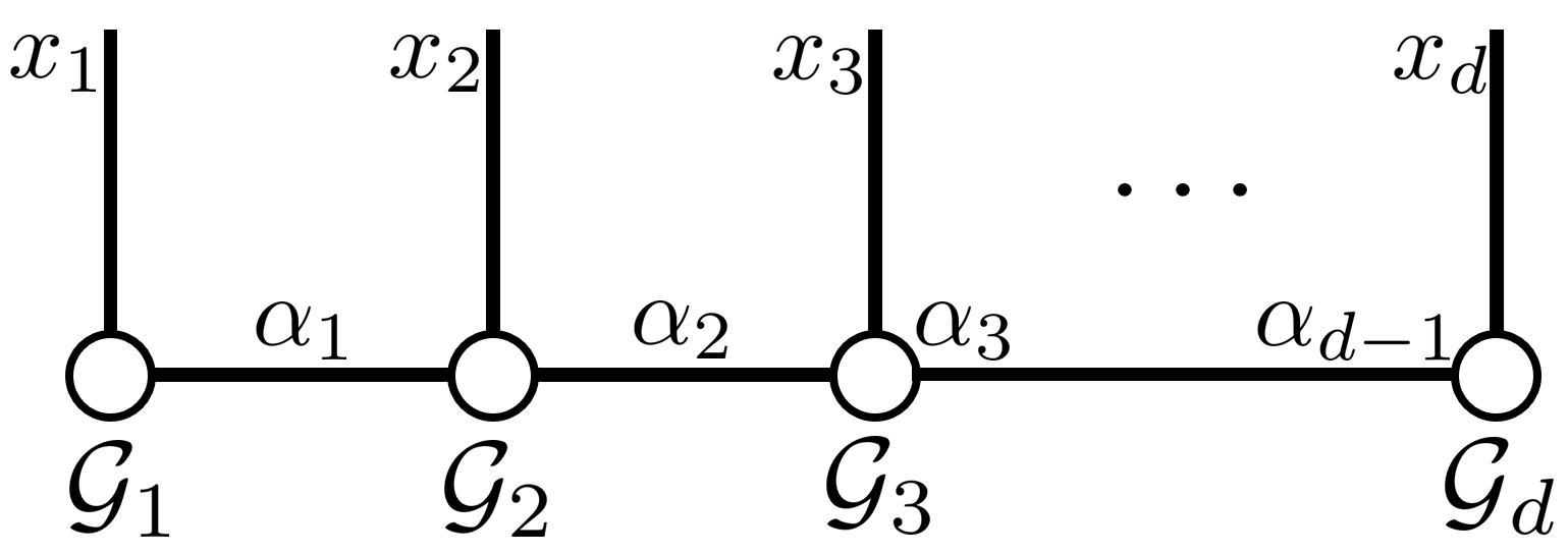
(a) MPS/TT

(b) MPO

Figure 2.1. Tensor diagram for a $d$-dimensional MPS/TT and MPO. (a): An MPS/TT representing $u$ in Definition 1. The exposed legs indicates the MPS/TT takes $x_{1},\ldots,x_{d}$ as inputs, and the connected legs indicate the summation over $\alpha_{1},\ldots,\alpha_{d-1}$. (b) An MPO representing $O$. Each tensor core has two exposed legs pointing upwards and downwards, respectively, indicating two free dimensions.

Finally, we introduce some indexing conventions. For two integers $m,n\in\mathbb{N}$ where $n>m$, we use the MATLAB notation $m:n$ to denote the set $\{m,m+1,\cdots,n\}$. When working with high-dimensional functions, it is often convenient to group the variables into two subsets and think of the resulting object as a matrix. We call these matrices unfolding matrices. In particular, for $k=1,\cdots,d-1$, we define the $k$-th unfolding matrix by $u(x_{1},\cdots,x_{k};x_{k+1},\cdots,x_{d})$ or $u(x_{1:k};x_{k+1:d})$, which is obtained by grouping the first $k$ and last $d-k$ variables to form rows and columns, respectively.

2.2. Tensor Network Operations

In this subsection, we introduce several tensor network operations of high importance in our applications using the example of MPS/TT. Similar operators can be extended to more general tensor networks.

2.2.1. Marginalization

To marginalize the MPS/TT representation of $u$ defined in Definition 1, one can perform direct operations on each node $\mathcal{G}_{k}$. For instance, if the goal is to integrate out a specific variable $x_{k}$, the operation can be achieved by taking the summation:

(2.4) $$\sum_{x_{k}}\mathcal{G}_{k}(\alpha_{k-1},x_{k},\alpha_{k}).$$

The overall computational cost of the marginalization process is at most $O(d)$, depending on the number of variables that need to be integrated out.

2.2.2. Normalization

Often, one needs to compute the norm

$$\|u\|_{2}^{2}=\sum_{x_{1},\ldots,x_{d}}u(x_{1},\ldots,x_{d})^{2},$$

for a MPS/TT. One can again accomplish this via operations on each node. In particular, one can first form the Hadamard product $u\odot u$ in terms of two MPS/TTs, and then integrate out all variables $x_{1},\ldots,x_{d}$ of $u\odot u$ to get $\|u\|_{2}^{2}$ using marginalization of MPS/TT as described in Section 2.2.1. The complexity of forming the Hadamard product of two MPS/TTs is $O(d)$, as mentioned in [oseledets2011tensor]. Therefore, the overall complexity of computing $\|u\|_{2}^{2}$ using the described approach is also $O(d)$.

2.2.3. Sampling From MPS/TT Parametrized Probability Density

If given a density function $u(x_{1},x_{2},\dots,x_{d})$ in MPS/TT format, it is possible to exploit the linear algebra structure to draw independent and identically distributed (i.i.d.) samples in $O(d)$ time [dolgov2020approximation], thereby obtaining a sample $(y_{1},y_{2},\dots,y_{d})\sim u$. This approach is derived from the following identity:

(2.5) $$u(x_{1},x_{2},\dots,x_{d})=u(x_{1})u(x_{2}|x_{1})u(x_{3}|x_{2},x_{1})\dots u(x_{d}|x_{d-1},\dots,x_{1}),$$

where each

$$u(x_{i}|x_{i-1},\dots,x_{1})=\frac{u(x_{1:i})}{u(x_{1:i-1})},$$

is a conditional distribution of $u$. We note that it is easy to obtain the marginals $u(x_{1}),\ldots u(x_{1:d-1})$ (hence the conditionals) in $O(d)$ time. If we have such a decomposition (2.5), we can draw a sample $y$ in $O(d)$ complexity as follows. We first draw component $y_{1}\sim u(x_{1})$. Then we move on and draw $y_{2}\sim u(x_{2}|x_{1}=y_{1})$. We continue this procedure until we draw $y_{d}\sim u_{d}(x_{d}|x_{1:d-1}=y_{1:d-1})$.

2.3. Tensor-network sketching

In this subsection, we present a parallel method for obtaining the tensor cores for representing a $d$-dimensional function $u(x)$ that is discretely valued, i.e. each $x_{j}$ takes on finite values in a set $X_{j}$, as an MPS/TT. This is done via an MPS/TT sketching technique proposed in [hur2022generative] where the key idea is to solve a sequence of core determining equations. Let $u_{k}:X_{1}\times\cdots\times X_{k-1}\times\Gamma_{k-1}\rightarrow\mathbb{R},k=2,\ldots,d$ be a set of functions such that $\text{Range}(u_{k}(x_{1:k};\gamma_{k}))=\text{Range}(p(x_{1:k};x_{k+1:d}))$. In this case, a representation of $u$ as Definition 1 can be obtained via solving $\mathcal{G}_{k}$ from the following set of equations

(2.6) $$u_{1}(x_{1},\gamma_{1}) =\mathcal{G}_{1}(x_{1},\gamma_{1}),$$

(2.7) $$u_{k}(x_{1:k},\gamma_{k}) =\sum_{\gamma_{k-1}\in\Gamma_{k-1}}u_{k-1}(x_{1:k-1},\gamma_{k-1})\mathcal{G}_{k}(\gamma_{k-1},x_{k},\gamma_{k}),$$

$$u(x) =\sum_{\gamma_{d-1}\in\Gamma_{d-1}}u_{d-1}(x_{1:d-1},\gamma_{d-1})\mathcal{G}_{k}(\gamma_{d-1},x_{d}),$$

based on knowledge of $u_{k}$’s.

However (2.6) is still inefficient to solve since each $u_{k}$ is exponentially sized, moreover, such a size prohibits it to be obtained/estimated in practice. Notice that (2.6) is over-determined, we further reduce the row dimensions by applying a left sketching function to (2.6),

(2.8) $$\sum_{x_{1}}\cdots\sum_{x_{k-1}}S_{k-1}(x_{1:k-1},\xi_{k-1})u_{k}(x_{1:k},\gamma_{k})$$

$$= \sum_{\gamma_{k-1}\in\Gamma_{k-1}}\left(\sum_{x_{1:k-1}}S_{k-1}(x_{1:k-1},\xi_{k-1})u_{k-1}(x_{1:k-1},\gamma_{k-1})\right)\mathcal{G}_{k}(\gamma_{k-1},x_{k},\gamma_{k}),$$

where $S_{k-1}:X_{1}\times\cdots\times X_{k-1}\times\Xi_{k-1}\rightarrow\mathbb{R}$ is the left sketching function which compresses over variables $x_{1},\cdots,x_{k-1}$.

Now to obtain $u_{k}$ where $\text{Range}(u_{k}(x_{1:k};\gamma_{k}))=\text{Range}(u(x_{1:k};x_{k+1:d}))$, we use a right-sketching by sketching the dimensions $x_{k+1:d}$, i.e.

(2.9) $$u_{k}(x_{1:k},\gamma_{k})=\sum_{x_{k+1:d}}u(x_{1:k},x_{k+1:d})T_{k+1}(x_{k+1:d},\gamma_{k}),$$

where $T_{k+1}:X_{k+1}\times\cdots\times X_{d}\times\Gamma_{k}\rightarrow\mathbb{R}$ is the right sketching function which compresses $u$ by contracting out variables $x_{k+1},\cdots,x_{d}$. Plugging such a $u_{k}$ into (2.6), we get

(2.10) $$B_{k}[u](\xi_{k-1},x_{k},\gamma_{k})=\sum_{\gamma_{k-1}\in\Gamma_{k-1}}A_{k}[u](\xi_{k-1},\gamma_{k-1}){\mathcal{G}_{k}}(\gamma_{k-1},x_{k},\gamma_{k}),$$

where

(2.11) $$A_{k}[u](\xi_{k-1},\gamma_{k-1}) =\sum_{x_{1:k-1}}\sum_{x_{k:d}}S_{k-1}(x_{1:k-1},\xi_{k-1})u(x_{1:k-1},x_{k:d})T_{k}(x_{k:d},\gamma_{k-1}),$$

(2.12) $$B_{k}[u](\xi_{k-1},x_{k},\gamma_{k}) =\sum_{x_{1:k-1}}\sum_{x_{k+1:d}}S_{k-1}(x_{1:k-1},\xi_{k-1})u(x_{1:k-1},x_{k},x_{k+1:d})T_{k+1},(x_{k+1:d},\gamma_{k}),$$

and we can readily solve for $\mathcal{G}_{k}$.

Many different types of sketch functions can be used, e.g. random tensor sketches or cluster basis sketches [ahle2019almost, wang2015fast]. Take a single $S_{k}(x_{1:k},\xi_{k})$ as an example, we choose a separable form $S_{k}(x_{1:k},\xi_{k})=h_{1}(x_{1})\cdots h_{k}(x_{k})$ for some $h_{1},\ldots,h_{k}$ (and similarly for $T_{k}$’s) in order to perform fast tensor operations. When the state space is discrete, random tensor sketch amounts to taking $h_{1},\cdots,h_{k}$ to be random vectors of size $|X_{1}|,\ldots,|X_{k}|$.

We give special focus to cluster basis sketch, defined as the following:

Definition 3.

Let $\{b_{l}\}_{l=1}^{n}$ be a set of single variable basis. A cluster basis sketch with $c$-cluster consists of choosing $S_{k}(x_{1:k},\xi_{k})\in\left\{b_{l_{1}}(x_{i_{1}})\cdots b_{l_{c}}(x_{i_{c}})\ |\ (l_{1},\ldots,l_{c})\in[n]^{c},\ \{x_{i_{1}},\ldots,x_{i_{c}}\}\subseteq\{x_{1},\ldots,x_{k}\}\right\}$, and also $T_{k}(x_{k:d},\gamma_{k-1})\in\left\{b_{l_{1}}(x_{i_{1}})\cdots b_{l_{c}}(x_{i_{c}})\ |\ (l_{1},\ldots,l_{c})\in[n]^{c},\ \{x_{i_{1}},\ldots,x_{i_{c}}\}\subseteq\{x_{k},\ldots,x_{d}\}\right\}$. For convenience, $S_{k},T_{k}$’s are chosen to be orthogonal basis.

A similar construct is used in [peng2023generative]. In this case, $A_{k}$ is of size estimate ${k-1\choose c}n^{c}\times{d-k+1\choose c}n^{c}$, and $B_{k}$ is of size ${k-1\choose c}n^{c}\times|X_{k}|\times{d-k+2\choose c}n^{c}$. In principle, we only need ${d-k+2\choose c}n^{c}>r$ for determining a rank-$r$ MPS/TT, therefore in practice $c\leq 2$ meets the need. The most important property we look for is that the variance $A_{k}[\hat{u}],B_{k}[\hat{u}]$ is small, if $\hat{u}$ is an unbiased estimator of $u$. As we shall see in Section 5, when $u$ is a density and $\hat{u}$ is an empirical distribution with $N$ samples approximating $u$, the choice of such a cluster basis results in the standard deviation of $A_{k}[\hat{u}],B_{k}[\hat{u}]$ being $O\left(\frac{n^{2c+1}}{\sqrt{N}}\right)$. In contrast, if one chooses a randomized function that involves all $d$ variables as a sketch, the variance would be $O(n^{d}/\sqrt{N})$.

Remark 1 (Rank of the MPS/TT representation).

The rank of the MPS/TT may be too large due to oversketching. For instance, when using a cluster basis sketch with a fixed cluster size, the core determining matrices can grow polynomially with the total number of dimensions. However, the intrinsic rank of the MPS/TT may be small. To address this issue, we can utilize truncated singular value decompositions (SVD) of the matrices $\{A_{k}[u]\}_{k=2}^{d}$ to define projectors that reduce the rank of the MPS/TT representation. Let

(2.13) $$A_{k}[u](\xi_{k-1},\gamma_{k-1})=\sum_{\alpha_{A,k-1}=1}^{r_{A,k-1}}U_{A,k}(\xi_{k-1},\alpha_{A,k-1})S_{A,k}(\alpha_{A,k-1},\alpha_{A,k-1})V_{A,k}^{T}(\alpha_{A,k-1},\gamma_{k-1}),\ \ k=2,\dots,d$$

be the truncated SVD with rank $r_{A,k-1}$ for $A_{k}[u]$. By solving (2.10) with such a truncation, we obtain an MPS/TT with tensor cores $\{\mathcal{G}_{k}\}_{k=1}^{d}$ (see Fig. 2(a)). We can further insert projectors $\{V_{A,k}V_{A,k}^{T}\}_{k=2}^{d}$ between all cores to get the “trimmed” MPS/TT, as shown in Fig. 2(b). We use thick legs to denote dimensions with a large number of indices ($\gamma_{k}$’s) and thin legs to denote dimensions with a small number of indices ($\alpha_{A,k}$’s). Then we can redefine the reduced tensor cores by grouping the tensor nodes

$$\bar{\mathcal{G}}_{k}\coloneqq\sum_{\gamma_{k-1}}\sum_{\gamma_{k}}V_{A,k}^{T}(\alpha_{A,k-1},\gamma_{k-1})\mathcal{G}_{k}(\gamma_{k-1},x_{k},\gamma_{k})V_{A,k+1}(\gamma_{k},\alpha_{A,k}),\ \ k=2,\dots,d-1,$$

(2.14) $$\text{and}\ \bar{\mathcal{G}}_{1}\coloneqq\sum_{\gamma_{1}}\mathcal{G}_{1}(x_{1},\gamma_{1})V_{A,2}(\gamma_{1},\alpha_{A,1}),\ \bar{\mathcal{G}}_{d}\coloneqq\sum_{\gamma_{d-1}}V_{A,d}^{T}(\alpha_{A,d},\gamma_{d})\mathcal{G}_{d}(x_{d},\gamma_{d-1}).$$

The regrouping operations are highlighted with red dashed boxes in Fig. 2(b). Now the new tensor core $\bar{\mathcal{G}}_{k}$ is of shape $r_{A,k-1}\times|X_{k}|\times r_{A,k}$ (Fig. 2(c)). We reduce the bond dimensions of the original MPS/TT $(|\Gamma_{1}|,\dots,|\Gamma_{d-1}|)$ to $(r_{A,1},\dots,r_{A,{d-1}})$.

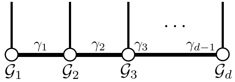
(a) Original MPS/TT

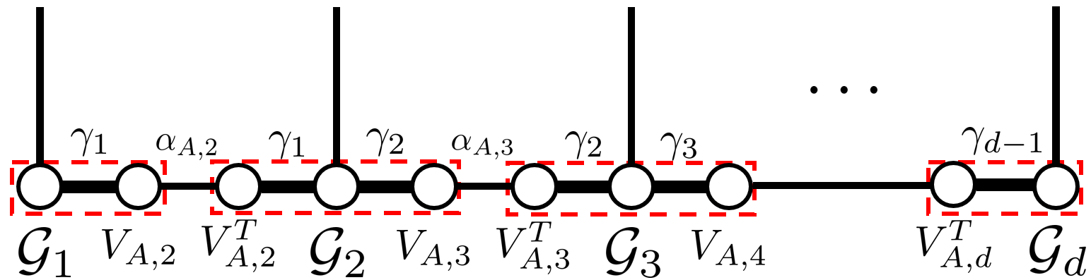
(b) Insert projectors and regrouping

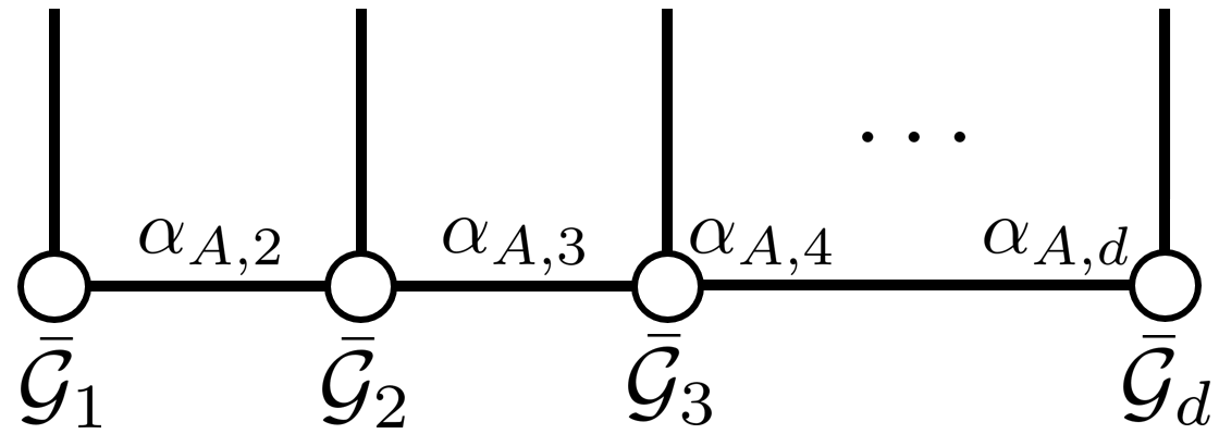
(c) Reduced MPS/TT

Figure 2.2. Tensor diagrams to reduce the bond dimensions of MPS/TT via truncated SVD. The regrouping operation for each reduced tensor $\bar{\mathcal{G}}_{k}$ is highlighted by red dashed boxes.

3. Proposed Framework

In this section, we present a framework for solving time-evolving systems that arise in both statistical and quantum mechanical systems. In many applications, the evolution of a $d$-dimensional physical system in time is described by a PDE of the form,

(3.1) $$\frac{\partial\phi(x,t)}{\partial t}=-A\phi(x,t),\ t\geq 0,\ \phi(x,0)=\phi_{0}(x),$$

where $A$ is a positive-semidefinite operator and has a semigroup $\{\exp{(-At)}\}_{t}$ [clifford1961algebraic, hollings2009early, howie1995fundamentals]. $x=(x_{1},x_{2},\cdots,x_{d})$ is a $d$-dimensional spatial point. Depending on the problem, $\phi(x,t)$ might be constrained to some sets. The solution of (3.1) can be obtained by applying the semigroup operator $\exp{(-At)}$ to the initial function, i.e. $\phi(x,t)=\exp(-At)\phi_{0}(x)$ for all $t\in\mathbb{R}$. We are especially interested in obtaining the stationary solution $\phi^{*}=\phi(\cdot,t),t\rightarrow\infty$. When (3.1) is a Fokker-Planck equation, $\phi^{*}$ corresponds to the equilibrium distribution of Langevin dynamics. When (3.1) is the imaginary time evolution of a Schrödinger equation, $\phi^{*}$ is the lowest energy state wavefunction.

Our method alternates between the two steps detailed in Alg. 1. Notice that we introduce three versions of the state $\phi$: $\phi_{t}$ is the ground truth state function at time $t$; $\hat{\phi}_{t}$ is a particle approximation of $\phi_{t}$; $\phi_{\theta_{t}}$ is a tensor-network representation of $\phi_{t}$. The significance of these two operations can be described as follows. In the first step, we use a particle-based simulation to bypass the need of applying $\exp(-A\delta t)\phi_{\theta_{t}}$ exactly, which may have a computational cost that scales unfavorably with respect to the dimensionality. In particular, we generate $f(x;x^{i})$ that can be represented easily as a low-rank TT. In the second step, the use of the sketching algorithm [hur2022generative] bypasses a direct application of recursive SVD-based compression scheme [oseledets2011tensor], which may run into $O(dN^{2})$ complexity. From a statistical complexity point of view, the variance of an empirical distribution $\text{Var}(\hat{\phi}_{t+1})$ scales exponentially in $d$, therefore one cannot apply a standard tensor compression scheme to $\hat{\phi}_{t+1}$ directly since it preserves the exponential statistical variance. Hence it is crucial to use the techniques proposed in [hur2022generative], which is designed to control the variance of the sketching procedure.

The method to obtain a Monte-Carlo representation of the time-evolution in Step 1 of Alg. 1 is dependent on the applications, and we present different schemes for many-body Schrödinger and Fokker-Planck equation in Section 4. In this section, we focus on the details of the second step.

Algorithm 1 Combining tensor-network and Monte-Carlo method by sketching

1:Apply the semigroup operator $\exp(-A\delta t)$ to the tensor-network approximation of the solution $\phi_{\theta_{t}}(x)$ using particle simulations for $\delta t>0$, i.e.

(3.2) $$\phi_{t+1}(x)=\exp{(-A\delta t)}\ \phi_{\theta_{t}}(x)=\mathbb{E}_{y\sim\mu}[f(x;y)]\approx\frac{1}{N}\sum_{i=1}^{N}f(x;x^{i})=:\hat{\phi}_{t+1}(x),$$

where $\{x^{i}\}_{i=1}^{N}\subset\mathbb{R}^{d}$ is a collection of $N$ i.i.d. samples according to a distribution $\mu$ (depending on the application, see Section 4 and $f(x;x^{i})$ is a $d$-dimensional function with parameters $x^{i}$. In the traditional Monte Carlo simulation, $f$ is simply the Dirac delta function at the given sample point, i.e. $f(x;x^{i})=\delta(x-x^{i})$.

2:Estimate $\phi_{t+1}(x)$ as a tensor-network $\phi_{\theta_{t+1}}(x)$ from its particle approximations $\hat{\phi}_{t+1}(x)$ via the parallel TT-sketching method with linear time complexity with respect to the number of samples and constant time with respect to the dimension if distributed computing is used (Section 2.3). Often certain normalization constraints (with respect to a certain norm $\|\cdot\|$) need to be enforced for $\phi_{\theta_{t+1}}$. In this case one simply adds an extra step, letting $\phi_{\theta_{t+1}}\leftarrow\frac{\phi_{\theta_{t+1}}}{\|\phi_{\theta_{t+1}}\|_{2}}$, which can be done with $O(d)$ complexity (Section 2.2.2).

3.1. MPS/TT Sketching for random walkers represented as a sum of TT

The concept of MPS/TT sketching or general tensor network sketching for density estimations has been extensively explored in [hur2022generative, ren2022high, tang2022generative]. The choice of tensor network representation in practice depends on the problem’s structure. In this work, we demonstrate the workflow using MPS/TT, but the framework can be readily extended to other tensor networks.

A crucial assumption underlying our approach is that each particle $f(x;x^{i})$ exhibits a simple structure and can be efficiently represented or approximated in MPS/TT format. For instance, in the case of a vanilla Markov Chain Monte Carlo (MCMC), we have $f(x;x^{i})=\delta(x-x^{i})=\prod_{j=1}^{d}\delta(x_{j}-x_{j}^{i})$, which can be expressed as a rank-1 MPS/TT. Consequently, the right-hand side of (3.2) becomes a summation of $N$ MPS/TTs. The tensor diagram illustrating this general particle approximation is shown in Fig. 1(a). A naive approach for representing this sum as an MPS/TT consists of directly adding these MPS/TTs, which yields an MPS/TT with a rank of $N$ [oseledets2011tensor]. This growth in rank with the number of samples can lead to a high computational complexity of $O(\text{poly}(N))$ when performing tensor operations.

On the other hand, depending on the problem, if we know that the intrinsic MPS/TT rank of the solution is small, it should be possible to represent the MPS/TT with a smaller size. To achieve this, we apply the method described in Section 2.3 to estimate a low-rank tensor directly from the sum of $N$ particles. Specifically, we construct $A_{k}[\hat{\phi}_{t+1}]$ and $B_{k}[\hat{\phi}_{t+1}]$ from the empirical samples $\hat{\phi}_{t+1}$ and use them to solve for the tensor cores through (2.10), resulting in $\phi_{\theta_{t+1}}$. This process is illustrated in Fig. 1(b), Fig. 1(c), and Fig. 1(d). It is important to note that we approximate the ground truth $\phi_{t+1}$ using stochastic samples $\hat{\phi}_{t+1}$. The estimated tensor cores form an MPS/TT representation of $\phi_{t+1}$, denoted as $\phi_{\theta_{t+1}}$.

3.2. Complexity Analysis

In this section, we assume we are given $\hat{\phi}_{t+1}$ in (3.1) as $N$ constant rank MPS/TT. In terms of samples, forming $A_{k}[\hat{\phi}_{t+1}])$ and $B_{k}[\hat{\phi}_{t+1}]$ in (2.11) and (2.12) can be done as

(3.3) $$A_{k}[\hat{\phi}_{t+1}](\xi_{k-1},\gamma_{k-1})$$

$$= \frac{1}{N}\sum_{i=1}^{N}\left[\sum_{x_{1:k-1}}\sum_{x_{k:d}}S_{k-1}(x_{1:k-1},\xi_{k-1})f(x_{1:k-1},x_{k:d};x^{i})T_{k}(x_{k:d},\gamma_{k-1})\right],$$

$$B_{k}[\hat{\phi}_{t+1}](\xi_{k-1},x_{k},\gamma_{k})$$

$$= \frac{1}{N}\sum_{i=1}^{N}\left(\sum_{x_{1:k-1}}\sum_{x_{k+1:d}}S_{k-1}(x_{1:k-1},\xi_{k-1})f(x_{1:k-1},x_{k},x_{k+1:d};x^{i})T_{k+1}(x_{k+1:d},\gamma_{k})\right).$$

$B_{k}$ is a $3$-tensor of shape $|\Xi_{k-1}|\times|X_{k}|\times|\Gamma_{k}|$. $A_{k}$ is a matrix of shape $|\Xi_{k-1}|\times|\Gamma_{k}|$. The size of the linear system is independent of the number of dimensions $d$ and the total number of particles $N$. The number of sketch functions $|\Xi_{k}|$ and $|\Gamma_{k}|$ are hyperparameters we can control. Let $n=\max_{k}|X_{k}|$, $\tilde{r}=\max_{k}\{|\Xi_{k}|,|\Gamma_{k}|\}$. First we consider the complexity of forming the core determining equations, i.e. evaluating $A_{k}$ and $B_{k}$. We note that the complexity is dominated by evaluating the tensor contractions between sketch functions $S_{k}$’s, right sketch functions $T_{k}$’s and samples $f(\cdot;x^{i})$’s. If the sample $f(\cdot;x^{i})$ and sketch functions $S_{k}(\cdot,\xi_{k})$, $T_{k}(\cdot,\gamma_{k-1})$ are in low rank MPS/TT representations, then the tensor contractions in the square bracket in (3.3) can be evaluated in $O(d)$ time. Each term in the summation $\sum_{i=1}^{N}$ can be done independently, potentially even in parallel, giving our final $A_{k}$’s and $B_{k}$’s. Taking all $d$ dimensions into account, the total complexity of evaluating $A_{k}$’s and $B_{k}$’s is $O(n\tilde{r}^{2}Nd)$.

Next, the complexity of solving the linear system (2.10) is $O(n\tilde{r}^{3})$. For all $d$ dimensions, the total complexity for solving the core determining equations is $O(n\tilde{r}^{3}d)$. Combing everything together, the total computational complexity for MPS/TT sketching for a discrete particle system is

(3.4) $$O(n\tilde{r}^{2}Nd)+O(n\tilde{r}^{3}d).$$

Remark 2.

MPS/TT sketching is a method to control the complexity of the solution via estimating an MPS/TT representation in terms of the particles. Another more conventional approach to reduce the rank of MPS/TT is TT-round [tt-decomposition]. With this approach, one can first compute the summation in Fig. 1(a) to form a rank $O(N)$ MPS/TT and round the resulting MPS/TT to a constant rank. There are two main drawbacks of this approach. Firstly, the QR decomposition in TT-round has complexity $O(N^{2})$. Secondly, TT-round tries to make $\phi_{\theta_{t+1}}\approx\hat{\phi}_{t+1}$, which at the same time makes $\text{Var}(\phi_{\theta_{t+1}}))\approx\text{Var}(\hat{\phi}_{t+1})$, and such an error can scale exponentially.

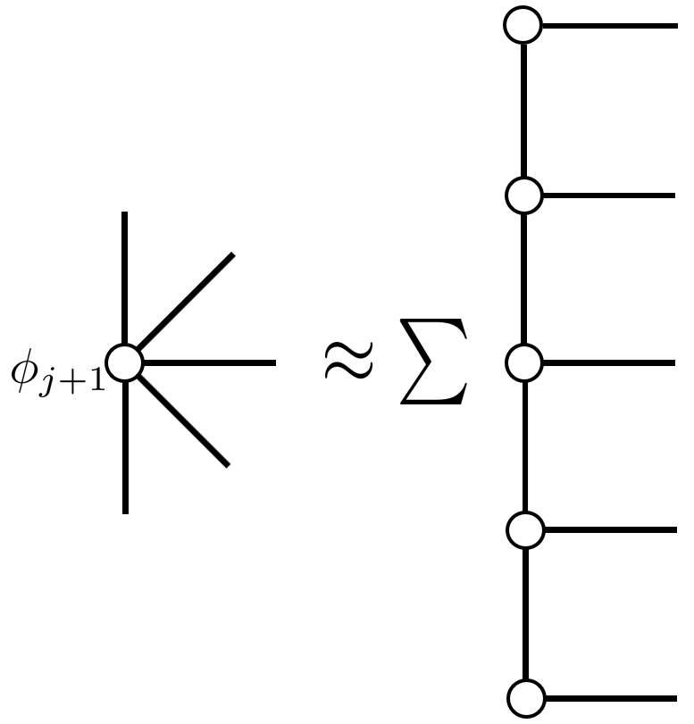
(a) Particle approximation of $\phi_{t+1}$

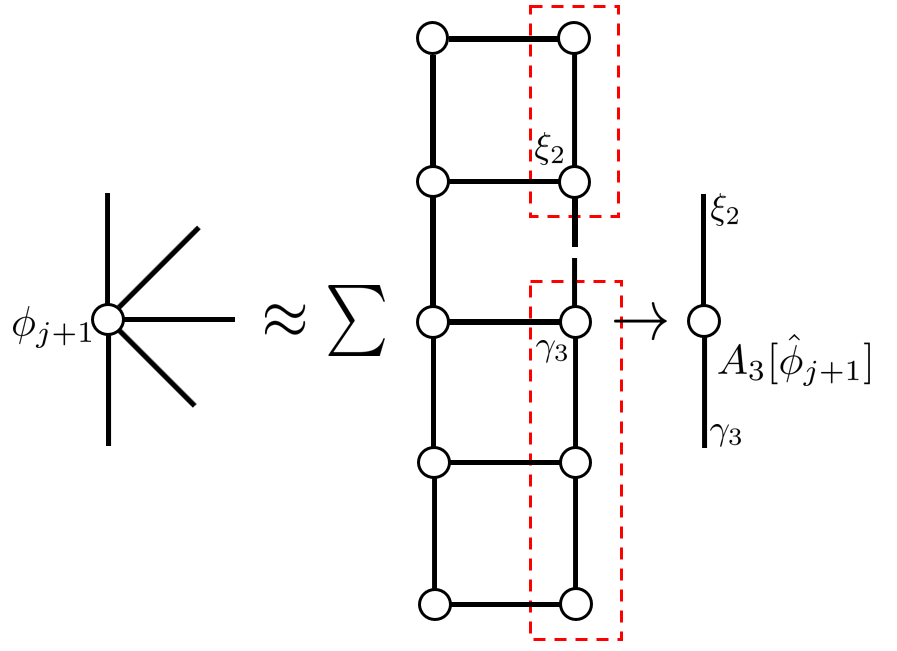
(b) Form $\{A_{k}\}_{k=1}^{d}$.

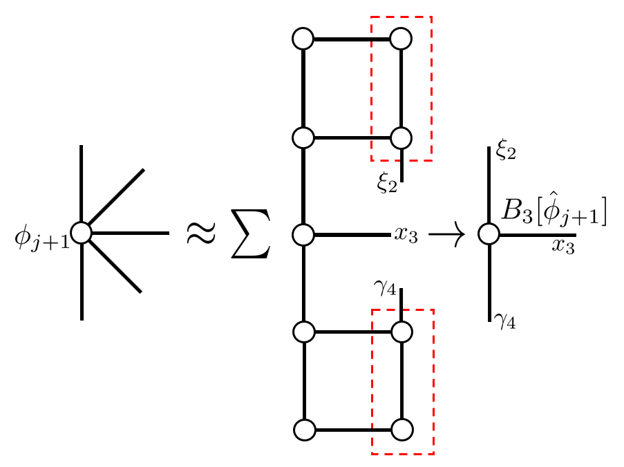
(c) Form $\{B_{k}\}_{k=1}^{d}$.

        

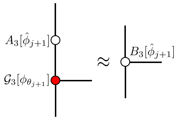
(d) Solving core determining equations

Figure 3.1. Tensor diagram for the workflow of estimating an MPS/TT from particles. Step (a) shows how $\phi_{t}$ is represented as empirical distribution $\hat{\phi}_{t+1}$. Step (b), (c), (d) shows how to form $A_{k}[\hat{\phi}_{t+1}],B_{k}[\hat{\phi}_{t+1}]$ in (3.3) and use them to solve for $\mathcal{G}_{k}$. Here we use the determination of $\mathcal{G}_{k}$ where $k=3$ as an example.

4. Applications

In this section, to demonstrate the generality of the proposed method, we show how it can be used in two applications: quantum Monte Carlo (Section 4.1) and solving Fokker-Planck equation (Section 4.2). For these applications, we focus on discussing how to approximate $\exp(-\beta A)\phi_{\theta_{t}}$ as a sum of MPS/TT, when $\phi_{\theta_{t}}$ is already in an MPS/TT representation, as required in (3.1).

4.1. Quantum Imaginary Time Evolutions

In this subsection, we apply the proposed framework to ground state energy estimation problems in quantum mechanics for the spin system. Statistical sampling-based approaches have been widely applied to these types of problems, see e.g. [lee2022unbiasing]. In this problem, we want to solve

(4.1) $$\frac{\partial\phi(x,t)}{\partial t}=-H\phi(x,t),\quad\|\phi(\cdot,t)\|_{2}=1$$

where $\phi(\cdot,t):\{\pm 1\}^{d}\rightarrow\mathbb{C}$, and $H$ is the Hamiltonian operator. Let $O:=[O_{i}]^{d}_{i=1}$, where

(4.2) $$O_{i}=I_{2}\otimes I_{2}\otimes\cdots\otimes\underbrace{\tilde{O}}_{\text{$i$-th term}}\otimes\cdots\otimes I_{2},$$

for some $\tilde{O}\in\mathbb{C}^{2\times 2}$, $O_{i}^{2}=I_{2^{d}}$, usually $H$ takes the form of $H_{1}[O]=\sum_{i=1}^{d}O_{i}$ or $H_{2}[O]=\sum_{i,j=1}^{d}J_{ij}O_{i}O_{j}$ or both. When $t\rightarrow\infty$, $\phi(\cdot,t)=\frac{\exp(-Ht)\phi_{0}}{\|\exp(-Ht)\phi_{0}\|_{2}}$ gives the lowest eigenvector of $H$. This can be done with the framework detailed in Section 3 with $A=H$. In what follows, we detail how $\exp(-\delta tH)\phi_{\theta_{t}}$ can be approximated as a sum of $N$ functions $f(x;x^{i})$ via a specific version of quantum Monte Carlo, the auxiliary-field quantum Monte Carlo (AFQMC). The AFQMC method [afqmc1, afmc2] is a powerful numerical technique that has been developed to overcome some of the limitations of traditional Monte Carlo simulations. AFQMC is based on the idea of introducing auxiliary fields to decouple the correlations between particles by means of the application of the Hubbard–Stratonovich transformation [hubbard1959calculation]. This reduces the many-body problem to the calculation of a sum or integral over all possible auxiliary-field configurations. The method has been successfully applied to a wide range of problems in statistical mechanics, including lattice field theory, quantum chromodynamics, and condensed matter physics [zhang2013auxiliary, carlson2011auxiliary, shi2021some, qin2016benchmark, lee2022twenty]. However, an issue of AFQMC is that the random walkers are biased towards a mean-field solution [qin2016coupling] in order to reduce the variance caused by the “sign problem”, giving rise to bias when determining the ground state energy. To solve this issue, [qin2016coupling] alternates between running AFQMC and determining a new mean-field solution in order to remove such a bias. Our approach can be regarded as a generalization to the philosophy in [qin2016coupling], where the mean-field is now replaced by a more general MPS/TT representation.

We first focus on how to apply $\exp(-\delta tH_{2}[O])$ where $H_{2}[O]=\sum^{d}_{i,j=1}J_{ij}O_{i}O_{j}$. We assume $J$ is positive semi-definite, which can be easily achieved by adding a diagonal to $J$ since $O_{i}^{2}=I_{2^{d}}$. To decouple the interactions through orthogonal transformations, we first perform an eigenvalue decomposition $J=U\text{diag}(\lambda)U^{T}$ and compute

(4.3) $$\exp{(-\delta tH_{2}[O])} =\exp\left(-\delta t\sum_{j=1}^{d}\lambda_{j}(u_{j}\cdot O)^{2}\right)=\prod^{d}_{j=1}\exp(-\delta t\lambda_{j}(u_{j}\cdot O)^{2})+O(\delta t^{2}),$$

where $U=[u_{1},\ldots,u_{j}],u_{j}\cdot O:=\sum_{i=1}^{d}u_{ji}O_{i}$. The approximation follows from Trotter-decomposition [hatano2005finding]. Using the identity

(4.4) $$\exp(-ax^{2})=\sqrt{\frac{1}{2\pi a}}\int^{\infty}_{-\infty}\exp\left(-\frac{k^{2}}{2a}\right)\exp(-ikx)dk,$$

we can write (4.3) as

(4.5) $$\exp(-\delta tH_{2}[O])= \int_{-\infty}^{\infty}\cdots\int_{-\infty}^{\infty}(2\pi)^{-d/2}\left(\prod_{j=1}^{d}\exp\left(-k_{j}^{2}/2\right)\right)$$

$$\left(\prod_{j=1}^{d}\exp\left(\sqrt{-2\delta t\lambda_{i}}k_{j}(u_{j}\cdot O)\right)\right)dk_{1}\cdots dk_{d}+O(\delta t^{2}).$$

Instead of sampling directly from the spin space, AFQMC approximates the $d$-dimensional integration in (4.5) by a Monte Carlo integration in the $k$-space. Replacing the integration with Monte Carlo samples, we get the following approximation,

(4.6) $$\exp(-\delta tH_{2}[O]) \approx\frac{1}{N}\sum_{i=1}^{N}\left(\prod_{j=1}^{d}\exp\left(\sqrt{-2\delta t\lambda_{j}}k^{i}_{j}(u_{j}\cdot O)\right)\right)+O(\delta t^{2})$$

$$\approx\frac{1}{N}\sum_{i=1}^{N}\exp(\sqrt{-1}(\tilde{k}^{i}\cdot O))+O(\delta t^{2})$$

where $N$ is the total number of Monte Carlo samples, $k^{i}_{j}$ is the $i$-th sample for the frequency variable of the $j$-th dimension, and $\tilde{k}^{i}=\sum^{d}_{j=1}\sqrt{2\delta t\lambda_{j}}k^{i}_{j}u_{j}$. All samples $\{k^{i}_{j}\}_{j=1,\cdots,d,\ i=1,\cdots,N}$ are drawn from i.i.d. standard normal distribution. The structure of such an approximation to $\exp(-\delta tH_{2}[O])$ is illustrated in Fig. 1(a), which is a sum of rank-1 MPO. The application of $\exp(-\delta tH_{2}[O])$ to a function $u$ that is already represented as an MPS/TT in the form of Def. 1 can written as

(4.7) $$\exp(-\delta tH_{2}[O])\phi_{t} \approx\frac{1}{N}\sum_{i=1}^{N}\left[\exp(\sqrt{-1}(\tilde{k}^{i}\cdot O))\phi_{t}\right].$$

Notably, since each $\exp(\sqrt{-1}(\tilde{k}^{i}\cdot O))$ is a rank-1 MPO, $\exp(\sqrt{-1}(\tilde{k}^{i}\cdot O))\phi_{t}$ has the same rank as $\phi_{t}$. Lastly, the application of $\exp(-\delta tH_{1}[O])$ to some $\phi_{t}$ that is represented as an MPS can be done easily, since $\exp(-\delta tH_{1}[O])=\prod_{i=1}^{d}\exp(-\delta tO_{i})$ is a rank-1 MPO.

To summarize, we can approximate the imaginary time propagator $\exp(-\delta t(H_{1}[O]+H_{2}[O]))$ with a summation of $N$ rank-$1$ MPOs. Applying the propagator to many-body wavefunction $\phi_{t}$ reduces to MPO-MPS contractions. The corresponding tensor diagram is shown in Fig. 1(b).

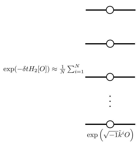
(a) MPO approximation of $\exp(-\delta tH_{2}[O])$

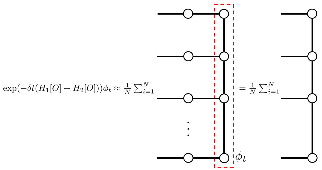
(b) MPS approximation of $\exp(-\delta t(H_{1}[O]+H_{2}[O]))\phi_{t}$

Figure 4.1. Tensor diagram for (a) approximating the imaginary time propagator $\exp(-\delta tH_{2}[O])$ as a summation of rank-$1$ MPO’s and (b) approximating evolution equation as MPO-MPS products. We remove the internal legs connecting the tensor cores in MPO to indicate the MPO has rank $1$.

4.2. Fokker-Planck equation

In this subsection, we demonstrate the application of the proposed framework to numerical simulations of parabolic PDEs, specifically focusing on the overdamped Langevin process and its corresponding Fokker-Planck equations. We consider a particle system governed by the following overdamped Langevin process,

(4.8) $$dx_{t}=-\nabla V(x_{t})\,dt+\sqrt{2\beta^{-1}}\,dW_{t},$$

where $x_{t}\in\Omega\subseteq\mathbb{R}^{d}$ is the state of the system, $V:\Omega\subset\mathbb{R}^{d}\rightarrow\mathbb{R}$ is a smooth potential energy function, $\beta=1/T$ is the inverse of the temperature $T$, and $W_{t}$ is a $d$-dimensional Wiener processs. If the potential energy function $V$ is confining for $\Omega$ (see, e.g., [bhattacharya2009stochastic, Definition 4.2]), it can be shown that the equilibrium probability distribution of the Langevin dynamics (4.8) is the Boltzmann-Gibbs distribution,

(4.9) $${\phi^{*}}(x)=\frac{1}{Z_{\beta}}\exp(-\beta V(x))$$

where $Z_{\beta}=\int_{\Omega}\exp(-\beta V(x))\,dx$ is the partition function. Moreover, the evolution of the distribution of the particle system can be described by the corresponding time-dependent Fokker-Planck equation,

(4.10) $$\frac{\partial\phi}{\partial t}=\beta^{-1}\Delta\phi+\nabla\cdot(\nabla V\phi)=:-A\phi,\quad\phi(x,0)=\phi_{0}(x),\quad\|\phi(\cdot,t)\|_{1}=1$$

where $\phi_{0}$ is the initial distribution. $\|\phi(\cdot,t)\|_{1}=1$ ensures that the $\int|\phi(x,t)|dx=1$. Therefore, (4.10) is the counterpart of (3.1) in our framework.

Now we need to be able to approximate $\exp(-A\delta t)\phi_{t}$ as particle systems. Assuming the current density $\phi_{t}$ is a MPS/TT, we use the following procedures to generate a particle approximation $\hat{\phi}_{t+1}$:

1. We apply conditional sampling on the current density estimate $\phi_{\theta_{t}}$ (Section 2.2.3) to generate $N$ i.i.d. samples $x^{1},\ldots,x^{N}\sim\phi_{\theta_{t}}$.

2. Then, we simulate the overdamped Langevin dynamics (4.8) using Euler-Maruyama method over time interval $\delta t$ for each of the $N$ initial stochastic samples $x^{1},\ldots x^{N}\sim\phi_{\theta_{t}}$. By the end of $\delta t$ we have final particle positions $x^{1},\ldots,x^{N}\sim\phi_{t+1}$, and

   (4.11) $$\hat{\phi}_{t+1}(x) =\frac{1}{N}\sum_{i=1}^{N}\delta(x-x^{i}),$$

by standard Monte Carlo approximation. Note that the only difference between this application and the quantum ground state problem is the conversion of the empirical distribution into an MPS/TT $\phi_{\theta_{t+1}}(x)$. Here, we employ a version of sketching for continuous distributions instead of discrete distributions as used in quantum ground state energy estimation (Section 4.1). For more detailed information on MPS/TT sketching for continuous distributions, we refer readers to Appendix C of [hur2022generative].

5. Convergence Analysis

In this section, we provide the convergence analysis for the proposed method. We look at the case for the Fokker-Planck equation, in a simplified discretized setting. Let $P_{\delta t}\in\mathbb{R}^{n^{d}\times n^{d}}$ be a Markov-transition kernel of a stochastic process on a discrete state space $[n]^{d}$. Denote the stationary distribution as $\phi^{\star}$, which satisfies $P_{\delta t}\phi^{\star}=\phi^{\star}$. We want to show that Alg. 1 converges to $\phi^{\star}$. To facilitate the discussion, we define a few new notations. For a $d$-tensor $u$ of size $n^{d}$, we define its “Frobenius norm” to be

(5.1) $$\|u\|_{F}:=\sqrt{\sum_{i_{1},\cdots,i_{d}}u(i_{1},\cdots,i_{d})^{2}}.$$

Furthermore, when representing $u$ as an MPS/TT with cores $\mathcal{G}_{1},\cdots,\mathcal{G}_{d}$, we use the notation

(5.2) $$u=\mathcal{G}_{1}\circ\mathcal{G}_{2}\cdots\circ\mathcal{G}_{d}.$$

We are also going to use a standard perturbation theory result for the solution of a linear system.

Lemma 1 (Theorem 3.48, [wendland2017numerical]).

Suppose $Ax^{\star}=b$, $A\in\mathbb{R}^{n\times n},b\in\mathbb{R}^{n\times 1}$. Further $(A+\Delta A)x=(b+\Delta b)$. Then with $\|A^{\dagger}\|_{2}\|\Delta A\|_{2}\leq 1$, we have

(5.3) $$\frac{\|x-x^{\star}\|}{\|x^{\star}\|}\leq\frac{\|A^{\dagger}\|_{2}}{1-\|A^{\dagger}\|_{2}\|\Delta A\|_{2}}(\|\Delta A\|_{2}+\|\Delta b\|_{2}/\|x^{\star}\|).$$

Our main theorem is stated in Theorem 1, which shows that the iterates in Alg. 1 are contracting towards the true solution, perturbed by some error. To prove it, we make the following assumption.

Assumption 1.

Let $P_{\delta t}\in\mathbb{R}^{n^{d}\times n^{d}}$ be a Markov-transition kernel of a stochastic process on a discrete state space $[n]^{d}$. We assume that it has eigenvalues $1=\lambda_{1}^{\delta t}>\lambda_{2}^{\delta t}\geq\lambda_{3}^{\delta t}\cdots$, and therefore has a unique top eigenvector $P_{\delta t}\phi^{\star}=\phi^{\star}$. Furthermore, $\min(\phi^{\star})>0$.

Such an assumption is important to characterize the contraction rate towards $\phi^{\star}$ in Alg 1:

Lemma 2.

Suppose in Alg. 1, $\|\phi_{\theta_{t}}-\phi_{t}\|_{F}\leq\tilde{\nu}$, then

(5.4) $$\|\phi_{\theta_{t}}-\phi^{\star}\|_{F}\leq a^{t}\|\phi_{\theta_{0}}-\phi^{\star}\|_{F}+\tilde{\nu}$$

where $a:=\frac{\max{\phi^{\star}}}{\min{\phi^{\star}}}\lambda_{2}^{\delta t}$ for $\delta t$ large enough such that $a<1$.

Proof.

We first recall several definitions in Alg. 1. Let $\phi_{t+1}=P_{\delta t}\phi_{\theta_{t}}$, $\hat{\phi}_{t+1}$ be an empirical distribution of $\phi_{t+1}$ with $N$ samples, which satisfies $\mathbb{E}(\hat{\phi}_{t+1})=\phi_{t+1}$. Let $\phi_{\theta_{t+1}}$ be an MPS/TT approximation of $\phi_{t+1}$, obtained from plugging $\hat{\phi}_{t+1}$ into (3.3).

First, under Assumption 1, standard results in Markov process (see for example [chen2000equivalence]) give

(5.5) $$\|\phi_{t+1}-\phi^{\star}\|_{2,{\phi^{\star}}^{-1}}=\|P_{\delta t}\phi_{\theta_{t}}-\phi^{\star}\|_{2,{\phi^{\star}}^{-1}}\leq\lambda_{2}^{\delta t}\|\phi_{\theta_{t}}-\phi^{\star}\|_{2,{\phi^{\star}}^{-1}}.$$

This further gives

(5.6) $$\|\phi_{t+1}-\phi^{\star}\|_{2}\leq\lambda_{2}^{\delta t}\frac{\max{\phi^{\star}}}{\min{\phi^{\star}}}\|\phi_{\theta_{t}}-\phi^{\star}\|_{2}.$$

Using (5.6) together with assuming $\|\phi_{\theta_{t}}-\phi_{t}\|_{F}\leq\tilde{\nu}$, we have

(5.7) $$\|\phi_{\theta_{t+1}}-\phi^{\star}\|_{2}\leq\lambda_{2}^{\delta t}\frac{\max{\phi^{\star}}}{\min{\phi^{\star}}}\|\phi_{\theta_{t}}-\phi^{\star}\|_{2}+\tilde{\nu}.$$

By applying induction to (5.7) we have the desired conclusion. ∎

In Lemma 2, the error $\tilde{\nu}$ is caused by approximation and variance error associated with representing the iterates of Alg. 1 as MPS/TT. To provide estimates to these errors, we define a notion that characterizes the nearness between a function $u$ and an MPS/TT:

Definition 4.

For $u:[n]^{d}\rightarrow\mathbb{R}$, we say it is $\epsilon$-identifiable with a rank-$r$ MPS/TT $u^{\star}$ if each of the associated $A_{k}[u]$ (defined in (2.13)) can be approximated by $\|A_{k}[u]-A_{k}[u^{\star}]\|_{2}\leq\epsilon\|A_{k}[u^{\star}]\|_{2},\|B_{k}[u]-B_{k}[u^{\star}]\|_{F}\leq\epsilon\|B_{k}[u^{\star}]\|_{F}$. Furthermore, $\|A_{k}[u^{\star}]^{\dagger}\|_{2}\|A_{k}[u^{\star}]\|_{2}\leq 1$.

This notion of nearness between a function and an MPS/TT can be turned into a $\|\cdot\|_{F}$ bound between them.

Lemma 3.

Let $u^{\star}$ be a rank-$r$ MPS/TT, represented by cores $\mathcal{G}_{1}^{\star},\cdots,\mathcal{G}_{d}^{\star}$. Let $\hat{u}$ be $\epsilon$-identifiable with $u^{\star}$ as defined in Def. 4, then solving (2.10) with $A_{k}[\hat{u}],B_{k}[\hat{u}]$ gives

(5.8) $$\|\mathcal{G}_{k}-\mathcal{G}^{\star}_{k}\|_{F}\leq\|\mathcal{G}^{\star}_{k}\|_{F}\nu(\epsilon),\quad\|u-u^{\star}\|_{F}\leq d\nu(\epsilon)(1+\nu(\epsilon))^{d}\prod_{k=1}^{d}\|\mathcal{G}_{k}^{\star}\|_{F}.$$

where $\nu(\epsilon):=\frac{2\epsilon}{1-\epsilon}$

Proof.

First,

$$\|\mathcal{G}_{k}-\mathcal{G}^{\star}_{k}\|_{F}$$

$$\leq \frac{\|A_{k}[u^{\star}]^{\dagger}\|_{2}}{1-\|A_{k}[u^{\star}]^{\dagger}\|_{2}\|A_{k}[u^{\star}]-A_{k}[\hat{u}]\|_{2}}2\|\mathcal{G}^{\star}_{k}\|_{F}\max\{\|A_{k}[u^{\star}]^{\dagger}-A_{k}[\hat{u}]^{\dagger}\|_{2},\|B_{k}[u^{\star}]-B_{k}[\hat{u}]\|_{F}/\|\mathcal{G}^{\star}_{k}\|_{F}\}$$

$$\leq \frac{\|A_{k}[u^{\star}]^{\dagger}\|_{2}}{1-\|A_{k}[u^{\star}]^{\dagger}\|_{2}\|A_{k}[u^{\star}]-A_{k}[\hat{u}]\|_{2}}2\|\mathcal{G}^{\star}_{k}\|_{F}\max\{\|A_{k}[u^{\star}]\|_{2},\|B_{k}[u^{\star}]\|_{F}/\|\mathcal{G}^{\star}_{k}\|_{F}\}\epsilon$$

$$\leq \frac{\|A_{k}[u^{\star}]^{\dagger}\|_{2}}{1-\|A_{k}[u^{\star}]^{\dagger}\|_{2}\|A_{k}[u^{\star}]-A_{k}[\hat{u}]\|_{2}}2\|\mathcal{G}^{\star}_{k}\|_{F}\max\{\|A_{k}[u^{\star}]\|_{2},\frac{\|A_{k}[u^{\star}]\|_{2}\|\mathcal{G}^{\star}_{k}\|_{F}}{\|\mathcal{G}^{\star}_{k}\|_{F}}\}\epsilon$$

$$\leq \frac{2\epsilon}{1-\epsilon}\|\mathcal{G}_{k}^{\star}\|_{F}$$

The first inequality is due to Lemma 1. The second inequality is due to the assumption of the lemma and Def 4. The last inequality is due to the Definition 4 where $\|A_{k}[u^{\star}]^{\dagger}\|_{2}\|A_{k}[u^{\star}]\|_{2}\leq 1$. Then using a telescoping sum, we have

$$\|u-u^{\star}\|_{F}$$

$$= \|\mathcal{G}_{1}\circ\mathcal{G}_{2}\circ\cdots\circ\mathcal{G}_{d}-\mathcal{G}^{\star}_{1}\circ\mathcal{G}^{\star}_{2}\cdots\circ\mathcal{G}^{\star}_{d}\|_{F}$$

$$= \|(\mathcal{G}_{1}-\mathcal{G}^{\star}_{1})\circ\mathcal{G}^{\star}_{2}\cdots\circ\mathcal{G}^{\star}_{d}\|_{F}+\|\mathcal{G}_{1}\circ(\mathcal{G}_{2}-\mathcal{G}_{2}^{\star})\circ\mathcal{G}^{\star}_{3}\circ\cdots\mathcal{G}^{\star}_{d}\|_{F}\cdots+\|\mathcal{G}_{1}\circ\cdots\mathcal{G}_{d-1}\circ(\mathcal{G}_{d}-\mathcal{G}^{\star}_{d})\|_{F}$$

$$\leq \|\mathcal{G}_{1}-\mathcal{G}^{\star}_{1}\|_{F}\|\mathcal{G}^{\star}_{2}\cdots\circ\mathcal{G}^{\star}_{d}\|_{F}+\|\mathcal{G}_{1}\|_{F}\|\mathcal{G}_{2}-\mathcal{G}_{2}^{\star}\|_{F}\|\mathcal{G}^{\star}_{3}\circ\cdots\mathcal{G}^{\star}_{d}\|_{F}\cdots+\|\mathcal{G}_{1}\circ\cdots\mathcal{G}_{d-1}\|_{F}\|\mathcal{G}_{d}-\mathcal{G}^{\star}_{d}\|_{F}$$

$$\leq \nu(\epsilon)\|\mathcal{G}_{1}^{\star}\|_{F}\|\mathcal{G}^{\star}_{2}\circ\cdots\circ\mathcal{G}^{\star}_{d}\|_{F}+\nu(\epsilon)\|\mathcal{G}_{1}\|_{F}\|\mathcal{G}_{2}^{\star}\|_{F}\|\mathcal{G}^{\star}_{3}\circ\cdots\circ\mathcal{G}^{\star}_{d}\|_{F}\cdots+\nu(\epsilon)\|\mathcal{G}_{1}\circ\cdots\circ\mathcal{G}_{d-1}\|_{F}\|G_{d}^{\star}\|_{F}$$

$$\leq d\nu(\epsilon)(1+\nu(\epsilon))^{d}\prod_{k=1}^{d}\|\mathcal{G}_{k}^{\star}\|_{F}.$$

∎

We are now ready to provide a proof of convergence for Alg 1:

Theorem 1.

Let the sketch $S_{k},T_{k}$’s in (2.11) (2.12) be coming from cluster basis (Def. 3). In Alg. 1, we assume for all $t$, $\phi_{t}$ is $\epsilon_{1}$-identifiable with $\phi^{\star}_{\theta_{t}}=\mathcal{G}_{1,t}^{\star}\circ\cdots\circ\mathcal{G}_{d,t}^{\star}$ that is rank-$r$. Then for $t\in[0,T]$, we have

(5.9) $$\|\phi_{\theta_{t}}-\phi^{\star}\|_{F}\leq a^{t}\|\phi_{\theta_{0}}-\phi^{\star}\|_{F}+2d\nu(\epsilon_{1}+\epsilon_{2})(1+\nu(\epsilon_{1}+\epsilon_{2}))^{d}c_{G}$$

with probability $1-\delta$ where

• $a:=\frac{\max{\phi^{\star}}}{\min{\phi^{\star}}}\lambda_{2}^{\delta t}$ for $\delta t$ large enough such that $a<1$.

• $\nu(\epsilon)=\frac{2\epsilon}{1-\epsilon}$.

• $\epsilon_{2}=O\left(\sqrt{\frac{n^{2c+1}\log\left(T{d\choose 2c+1}n^{2c+1}\right)}{N}}\right).$

• $c_{G}=\max_{t}\prod_{k=1}^{d}\|\mathcal{G}_{k,t}^{\star}\|_{F}.$

• $\delta=O(1/T{d\choose 2c+1}n^{2c+1}).$

Proof.

Assuming $\phi_{t}$ is $\epsilon_{1}$-identifiable with some $\phi_{\theta_{t}}^{\star}=\mathcal{G}^{\star}_{1,t}\circ\cdots\circ\mathcal{G}^{\star}_{d,t}$ that is of rank-$r$. By Lemma 3, this gives $\|\phi_{t}-\phi_{\theta_{t}}^{\star}\|_{2}\leq d\nu(\epsilon_{1})(1+\nu(\epsilon_{1}))^{d}c_{G}$. Suppose for now, the empirical distribution $\hat{\phi}_{t}$ of $\phi_{t}$ satisfies $\|A_{k}[\hat{\phi}_{t}]-A_{k}[\phi_{t}]\|_{F},\|B_{k}[\hat{\phi}_{t}]-B_{k}[\phi_{t}]\|_{F}\leq\epsilon_{2},\forall k\in[d]$. Then $\|A_{k}[\hat{\phi}_{t}]-A_{k}[\phi_{\theta_{t}}^{\star}]\|_{F}\leq\|A_{k}[\phi_{t}]-A_{k}[\phi_{\theta_{t}}^{\star}]\|_{F}+\|A_{k}[\hat{\phi}_{t}]-A_{k}[\phi_{t}]\|_{F}\leq\epsilon_{1}+\epsilon_{2}$ (and also $\|B_{k}[\hat{\phi}_{t}]-B_{k}[\phi_{\theta_{t}}^{\star}]\|_{F}\leq\epsilon_{1}+\epsilon_{2}$). This means $\hat{\phi}_{t}$ is $(\epsilon_{1}+\epsilon_{2})$-identifiable with $\phi_{\theta_{t}}^{\star}$. Since $\phi_{\theta_{t}}$ is the MPS/TT obtained from $A_{k}[\hat{\phi}_{t}],B_{k}[\hat{\phi}_{t}],k\in[d]$, by Lemma 3, we have $\|\phi_{\theta_{t}}-\phi_{\theta_{t}}^{\star}\|_{2}\leq d\nu(\epsilon_{1}+\epsilon_{2})(1+\nu(\epsilon_{1}+\epsilon_{2}))^{d}c_{G}$. By triangle inequality, $\|\phi_{\theta_{t}}-\phi_{t}\|_{2}\leq\|\phi_{\theta_{t}}-\phi_{\theta_{t}}^{\star}\|_{2}+\|\phi_{\theta_{t}}^{\star}-\phi_{t}\|_{2}\leq 2d\nu(\epsilon_{1}+\epsilon_{2})(1+\nu(\epsilon_{1}+\epsilon_{2}))^{d}c_{G}$.

In order to complete the proof, we now give the expression of $\epsilon_{2}$, which is due to the variance of $A_{k}[\hat{\phi}_{t}]$ and $B_{k}[\hat{\phi}_{t}]$. We first look at $B_{k}[\hat{\phi}_{t}]$ of the form (2.12). Notice that each pair of $S_{k-1}(\cdot,\xi_{k-1}),T_{k+1}(\cdot,\gamma_{k})$ involves at most $n^{2c}$ variables due to the choice of cluster basis. Therefore, the variance of a single entry $B_{k}[\hat{\phi}_{t}][\xi_{k-1},x_{k},\gamma_{k}]$ comes from a $(2c+1)$-marginal distribution ${\hat{\phi}}_{t,\mathcal{S}}(x_{\mathcal{S}})$ of ${\hat{\phi}}$ for a subset $\mathcal{S}\in[d]$ where $|\mathcal{S}|=2c+1$. Each samples in the empirical distribution ${\hat{\phi}}_{t,\mathcal{S}}$ is a Bernoulli random variable with probability ${\phi}_{t,\mathcal{S}}(x_{\mathcal{S}})$. Therefore, by Hoeffding’s inequality, for a fixed $x_{\mathcal{S}}$,

(5.10) $$\text{Pr}(|{\hat{\phi}}_{t,\mathcal{S}}(x_{\mathcal{S}})-{\phi}_{t,\mathcal{S}}(x_{\mathcal{S}})|\geq\epsilon)\leq\exp(-N\epsilon^{2}).$$

Now we want to bound $|{\hat{\phi}}_{t,\mathcal{S}}(x_{\mathcal{S}})-{\phi}_{t,\mathcal{S}}(x_{\mathcal{S}})|$ for every $x_{\mathcal{S}}\in[n]^{2c+1}$. With a union bound over $n^{2c+1}$ entries of ${\hat{\phi}}_{t,\mathcal{S}}$, this implies

(5.11) $$\frac{\|{\hat{\phi}}_{t,\mathcal{S}}-{\phi}_{t,\mathcal{S}}\|_{F}}{\|{\phi}_{t,\mathcal{S}}\|_{F}}\leq\frac{\|{\hat{\phi}}_{t,\mathcal{S}}-{\phi}_{t,\mathcal{S}}\|_{\infty}}{\|{\phi}_{t,\mathcal{S}}\|_{F}}\leq\sqrt{n^{2c+1}}\epsilon\quad\text{with probability}\ 1-n^{2c+1}\exp(-N\epsilon^{2}).$$

Now since $B_{k}[\hat{\phi}_{t}]$ consists of applying an orthogonal change of basis to $\hat{\phi}_{t,S}$ for an $\mathcal{S}\in[d]$ (due to our choice of cluster basis in Def. 3), we also have

(5.12) $$\frac{\|B_{k}[\hat{\phi}_{t}]-B_{k}[\phi_{t}]\|_{F}}{\|B_{k}[\phi_{t}]\|_{F}}\leq\sqrt{n^{2c+1}}\epsilon\quad\text{with probability}\ 1-n^{2c+1}\exp(-N\epsilon^{2}).$$

A similar bound on $\frac{\|A_{k}[\hat{\phi}_{t}]-A_{k}[\phi_{t}]\|_{F}}{\|A_{k}[\phi_{t}]\|_{F}}$ can be obtained likewise. Using (5.12) and applying a union bound over all subsets $\mathcal{S}\in[d]$ that contributes to the construction of $A_{k}[\hat{\phi}_{t}],B_{k}[\hat{\phi}_{t}]$, and for all time $t$, we get

(5.13) $$\frac{\|B_{k}[\hat{\phi}_{t}]-B_{k}[\phi_{t}]\|_{F}}{\|B_{k}[\phi_{t}]\|_{F}},\frac{\|A_{k}[\hat{\phi}_{t}]-A_{k}[\phi_{t}]\|_{F}}{\|A_{k}[\phi_{t}]\|_{F}}\leq\sqrt{n^{2c+1}}\epsilon,\quad k\in[d],t\in[T]$$

with probability $1-T{d\choose 2c+1}n^{2c+1}\exp(-N\epsilon^{2})$. Letting $\epsilon=O\sqrt{\frac{\log\left(T{d\choose 2c+1}n^{2c+1}\right)}{N}}$ and identifying $\epsilon_{2}=\sqrt{n^{2c+1}}\epsilon$ completes the proof. ∎

Remark 3.

A few remarks are in order. $\epsilon_{1}$ is the bias error committed by approximating the “true” solution $\phi_{t}$ by an MPS/TT (in terms of the notion defined in Def 4), which depends on the underlying physics of the problem. $\epsilon_{2}$ is the variance error of determining an MPS/TT from empirical distribution $\hat{\phi}_{t}$. From (5.9), it seems like we have surmounted the curse of dimensionality for solving a (discretized) high-dimensional Fokker-Planck equation, since the error of determining the true solution only grows linearly in $d$ for $\epsilon_{1}+\epsilon_{2}=o(1/d)$. However, while the variance error $\epsilon_{2}$ can be reduced by increasing the number of samples (and we only need samples $N\sim O(n^{4c+2})$ to have a good approximation), in practice when solving a high-dimensional PDE, the bias (approximation) error $\epsilon_{1}$ could be difficult to reduce. This is where the curse-of-dimensionality could enter.

6. Numerical Experiments

6.1. Quantum Ground State Energy Estimations

In this subsection, we consider the ground state energy estimation problem using the transverse-field Ising model of the following quantum Hamiltonian,

(6.1) $$H=-\sum_{i,j=1}^{d}J_{ij}S^{z}_{i}S^{z}_{j}-h\sum_{i}S^{x}_{i},$$

where $S^{z}_{j}$, $S^{x}_{j}$ are the Pauli matrices [gull1993imaginary],

(6.2) $$S^{z}_{j}=I_{2}\otimes I_{2}\otimes\cdots\otimes\underbrace{\begin{pmatrix}1&0\\ 0&-1\end{pmatrix}}_{\text{j-th dimension}}\otimes\cdots\otimes I_{2},$$

(6.3) $$S^{x}_{j}=I_{2}\otimes I_{2}\otimes\cdots\otimes\underbrace{\begin{pmatrix}0&1\\ 1&0\end{pmatrix}}_{\text{j-th dimension}}\otimes\cdots\otimes I_{2},$$

and $I_{2}$ is the $2\times 2$ identity matrix. When $h=1$, and $J$ is the adjacency matrix of a 1D cycle graph, the system undergoes a quantum phase transition. We consider three models under this category: (a) $d=16$ sites, (b) $d=32$ sites, and (c) $d=64$ sites. We also consider a 2D Ising system which is configured as (d) $d=16$ sites with $h=1$, and $J$ the adjacency matrix of a 2D periodic square lattice. For the 1D model, the dimensions of the MPS/TT are naturally ordered according to the sites on the 1D chain. In the 2D Ising model case, we use a space-filling curve [sagan2012space] to order the dimensions. For example, we show the space-filling curve and the ordering of MPS/TT dimensions in a $4\times 4$ lattices in Fig. 6.1.

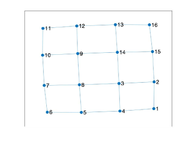
Figure 6.1. Example of $2$D space-filling curve for Ising model of $4\times 4$ lattices.

We set the infinitesimal time step $\delta t$ to be $0.01$, and use $2000$ samples in each power method iteration to approximate the propagator $\exp(-\delta tH)$. The rest of the parameters are set as follows: we use a $\tilde{r}=60$ (size of $|\Gamma_{k}|,|\Xi_{k}|$) random tensor sketches (Section 2.3) for sketching and we use $10^{-3}$ as the singular value threshold to solve the core determining equations (2.10). We initialize the initial wavefunction $\phi_{0}$ as a random MPS/TT. The imaginary time evolution energy is shown in Fig. 6.2. Here we use the symmetric energy estimator given by

(6.4) $$E_{\text{symmetric}}=\frac{\langle\phi_{t},H,\phi_{t}\rangle}{\langle\phi_{t},\phi_{t}\rangle},$$

where $\phi_{t}$ is the wavefunction of the $t$-th iteration. Theoretically, the energy given by the symmetric estimator can only be larger than the ground state energy. Often in quantum Monte-Carlo, mixed estimators

(6.5) $$E_{\text{mixed}}=\frac{\langle\phi,H,\phi_{t}\rangle}{\langle\phi,\phi_{t}\rangle},$$

where $\phi$ is a fixed reference wavefunction is used to reduce the bias error originating from the variance in $\phi_{t}$ [zhang2013auxiliary, shi2021some]. The variance can be further reduced by taking the average of the mixed energy estimators over several iterations.

(a) $d=16$ 1D transverse-field Ising symmetric estimator

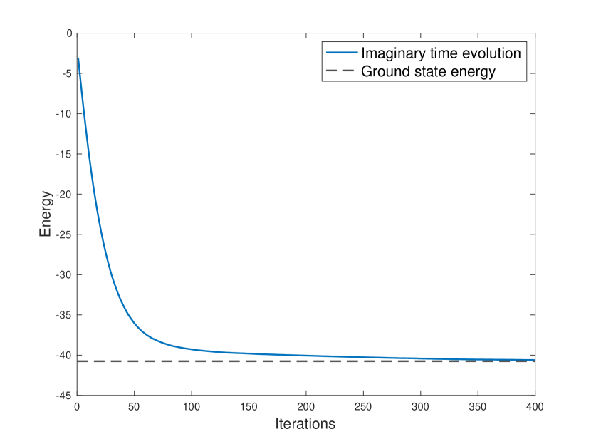
(b) $d=32$ 1D transverse-field Ising symmetric estimator

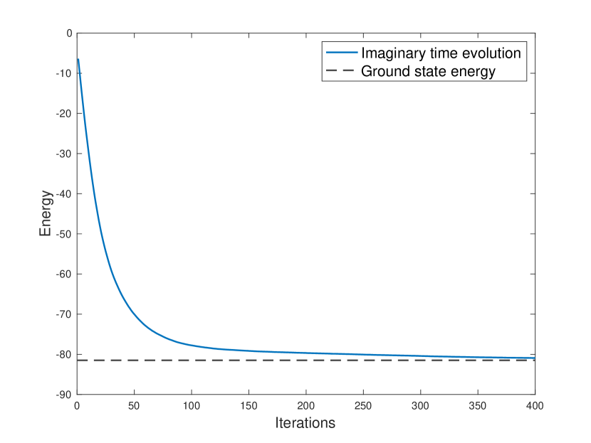
(c) $d=64$ 1D transverse-field Ising symmetric estimator

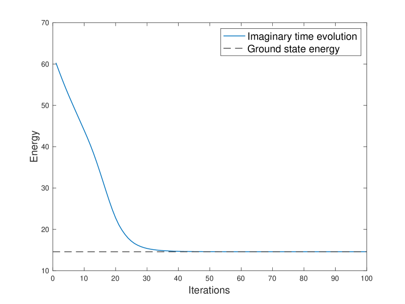
(d) $4\times 4$ 2D transverse-field Ising symmetric estimator

Figure 6.2. Imaginary time evolution energy plots. The ground state energy is shown as horizontal dashed lines.

We report the energies based on the symmetric estimator in Fig. 6.2 and compare with the ground truth energy for the quantum Hamiltonian. The ground state energy in 1D Ising model with $16$, $32$, and $64$ sites is reported in [sandvik2007variational]. For the $4\times 4$ 2D Ising model, we are still able to store the Hamiltonian exactly in memory so we solve the ground state energy by exact eigendecomposition.

For the 1D Ising model with $16$ sites, the ground-state energy per spin is $-1.2753$ and our approach converges to energy $-1.2751$, with a relative error of $1.86\times 10^{-4}$. For the 1D Ising model with $32$ sites, the ground-state energy per spin is $-1.2738$ and our approach converges to energy $-1.2726$, with a relative error of $9.10\times 10^{-4}$. For the 1D Ising model with $64$ sites, the ground-state energy per spin is $-1.2734$ and our approach converges to energy $-1.2712$, with a relative error of $1.67\times 10^{-3}$. In the 2D case, the ground-state energy per spin is $-0.6788$ and our approach converges to energy $-0.6744$, with a relative error of $6.5\times 10^{-3}$. Our approach has already achieved stable convergence and very accurate ground state energy estimation with only the symmetric estimators.

Next, we fix $J$ and test the performance of our proposed algorithm with a range of magnetic fields $h$. The results for $1D$ Ising model with $d=32$, $d=64$ sites and $2D$ Ising model with $d=16$ sites are summarized in Table 1, Table 2 and Table 3, respectively. The ground-state energy for 1D models can be exactly computed following [burkhardt1985finite, lieb1961two] and the energy for the 2D Ising model is computed by exact eigendecomposition. For all magnetic fields, our algorithm achieves stable convergence (not shown) and relative error in energy of order $\leq O(10^{-3})$.

	$h=0.2$	$h=0.6$	$h=1.0$	$h=1.4$	$h=1.8$
Ground-state energy per site	-1.0100	-1.0922	-1.2738	-1.5852	-1.9418
AFQMC+TT	-1.0100	-1.0921	-1.2726	-1.5846	-1.9411
Relative error	$7.51\times 10^{-6}$	$8.35\times 10^{-5}$	$9.10\times 10^{-4}$	$3.85\times 10^{-4}$	$3.44\times 10^{-4}$

Table 1. Estimation of ground-state energy per site for our proposed algorithm. In this table, we use 1D periodic boundary Ising model with $d=32$ sites for a range of magnetic field parameters $h$.

	$h=0.2$	$h=0.6$	$h=1.0$	$h=1.4$	$h=1.8$
Ground-state energy per site	-1.0100	-1.0922	-1.2734	-1.5852	-1.9418
AFQMC+TT	-1.0100	-1.0918	-1.2712	-1.5797	-1.9404
Relative error	$2.71\times 10^{-5}$	$3.78\times 10^{-4}$	$1.67\times 10^{-3}$	$3.44\times 10^{-3}$	$7.35\times 10^{-4}$

Table 2. Estimation of ground-state energy per site for our proposed algorithm. In this table, we use 1D periodic boundary Ising model with $d=64$ sites for a range of magnetic field parameters $h$.

	h=0.2	h=0.6	h=1.0	h=1.4	h=1.8
Ground-state energy per site	-1.5071	-1.5640	-1.6788	-1.8537	-2.0954
AFQMC+TT	-1.5071	-1.5639	-1.6786	-1.8531	-2.0945
Relative error	$6.62\times 10^{-6}$	$7.86\times 10^{-5}$	$1.25\times 10^{-4}$	$3.30\times 10^{-4}$	$3.88\times 10^{-4}$

Table 3. Estimation of ground-state energy per site for our proposed algorithm. In this table, we use $4\times 4$ 2D Ising model with $d=16$ sites for a range of magnetic field parameters $h$. The ground truth energy per site is computed by the exact eigendecomposition of the quantum Hamiltonian.

Tensor network sketching makes it possible to work with large number of samples while maintaining an algorithm with memory complexity that is independent of the number of samples. To demonstrate the advantage of tensor network sketching over other recompression methods, we consider a natural alternative that has constant memory usage. One can first add up the samples by performing addition in terms of MPS/TT into a high-rank tensor and truncate the rank. While doing addition, as the rank increases, if the rank hits 100 we apply the SVD-based TT-rounding procedure [oseledets2011tensor] to reduce the rank. The energy (computed by both the symmetric and mixed estimators) for $d=16$ 1D model and $4\times 4$ 2D Ising model are shown in Fig. 6.3. We can clearly observe that the energy convergence is more stable with the proposed sketching method.

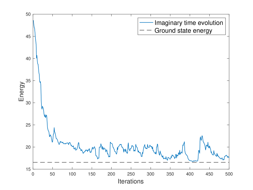
(a) $d=16$ 1D transverse-field Ising symmetric estimator

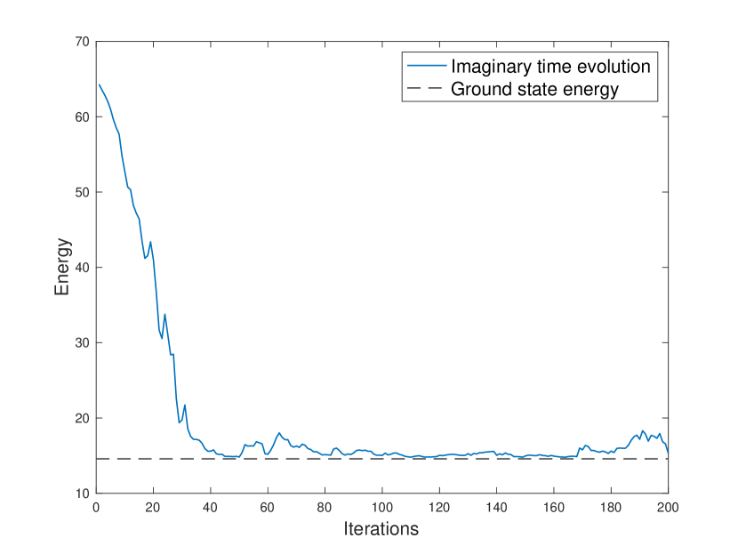
(b) $4\times 4$ 2D transverse-field Ising symmetric estimator

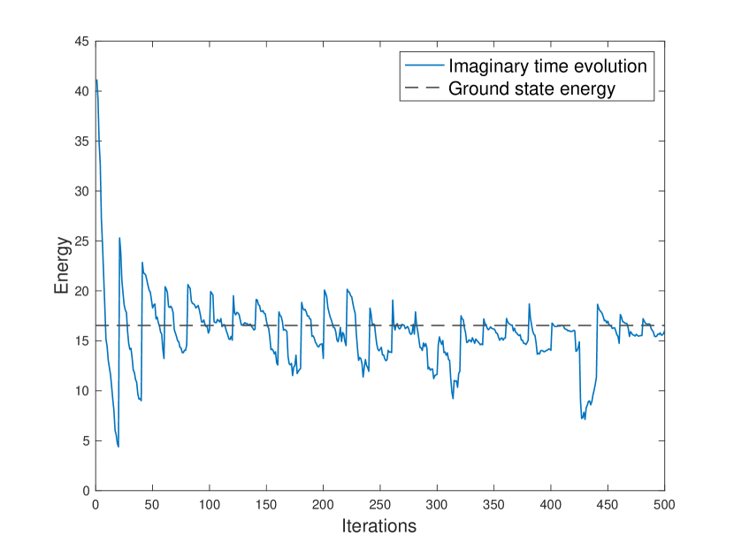
(c) $d=16$ 1D transverse-field Ising mixed estimator

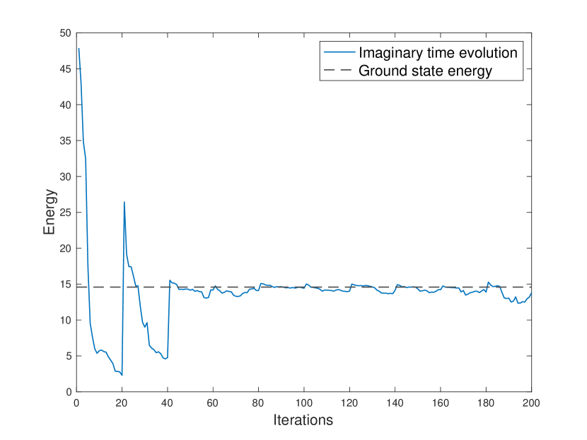
(d) $4\times 4$ 2D transverse-field Ising mixed estimator

Figure 6.3. Imaginary time evolution energy plots when iteratively adding and rounding the MPS/TT to constant rank.

6.2. Fokker-Planck Equation

In this numerical experiment, we solve the Fokker-Planck equation by parameterizing the density with MPS/TT. We consider two systems in this subsection, one with a simple double-well potential that takes a separable form, which is intrinsically a 1D potential, and the other one being the Ginzburg-Landau potential, where we only compare the obtained marginals with the ground truth marginals since the true density is exponentially sized.

6.2.1. Double-well Potential

We consider the following double-well potential

(6.6) $$V(x)=(x_{1}^{2}-1)^{2}+0.3\sum_{j=2}^{d}x_{j}^{2},$$

and the particle dynamics governed by overdamped Langevin equation (4.8). Since the potential function is easily separable, the equilibrium Boltzmann density is a product of univariate densities for each dimension, i.e.

(6.7) $$\frac{1}{Z_{\beta}}\exp(-\beta V(\bm{x}))=\frac{1}{Z_{\beta}}\exp\left(-\beta(x_{1}^{2}-1)^{2}\right)\prod_{j=2}^{d}\exp\left(-0.3\beta x_{j}^{2}\right).$$

In this example, we use $\beta=1$ and $d=10$. The support of the domain is a hypercube $[-M,M]^{d}$ where $M=2.5$. To obtain a continuous MPS/TT approximation, we use the Gaussian kernel function as univariate basis functions $\{b_{l}\}_{l=1}^{20}$, where

(6.8) $$b_{l}(\cdot)=\exp\left(-\frac{(\ \cdot\ +M-(l-1)\Delta x)^{2}}{2\Delta x^{2}}\right),\ l=1,\dots,20,$$

$\Delta x=5/18$ to form cluster basis for spanning the PDE solution, as mentioned in Section 2.3. In terms of the sketching function, we use cluster basis functions with $c=1,2$ as mentioned in 3. This results in $\tilde{r}=100$ tensor sketches. After sketching, we obtain a continuous analog of (2.10) (where each $\mathcal{G}_{k}$ is a set of continuous univariate functions), and we solve this linear least-squares in function space using the same set of univariate basis functions. We visualize all the basis functions in Fig. 6.4.

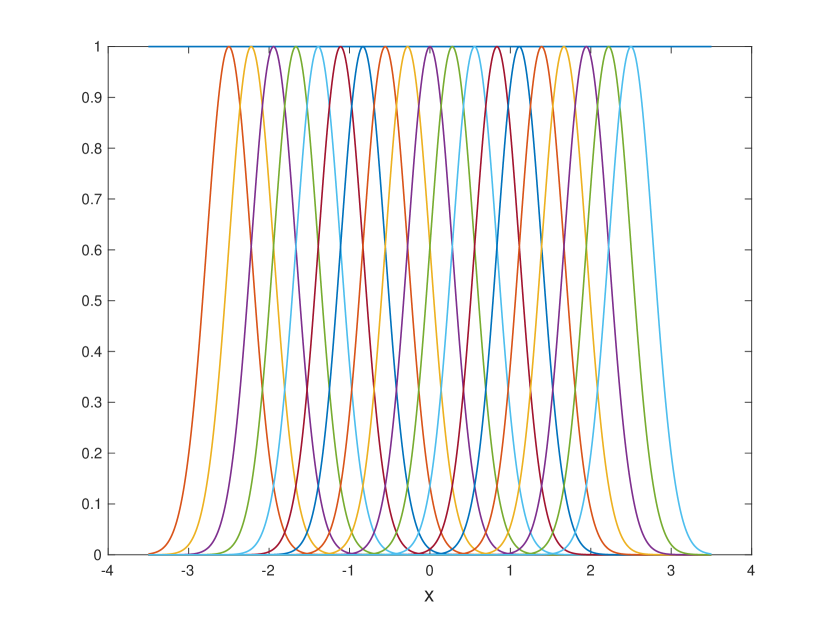
Figure 6.4. Visualization of univariate basis functions for each dimension. Here we use univariate Gaussian kernel functions as our basis functions.

We start from the uniform distribution over the hypercube $[-M,M]^{d}$ and evolve the distribution towards equilibrium. To approximate the given solution at each time $\phi_{\theta_{t}}$ as an MPS/TT, we first sample from this distribution via a conditional sampling Section 2.2.3. Then we simulate the overdamped Langevin process forward for the sampled particles up to time $\delta t$, as detailed in Section 4.2. Then we estimate a new MPS/TT representation $\phi_{\theta_{t+1}}$. We choose $\delta t=0.02$ time and we use $N=10^{4}$ samples for all iterations.

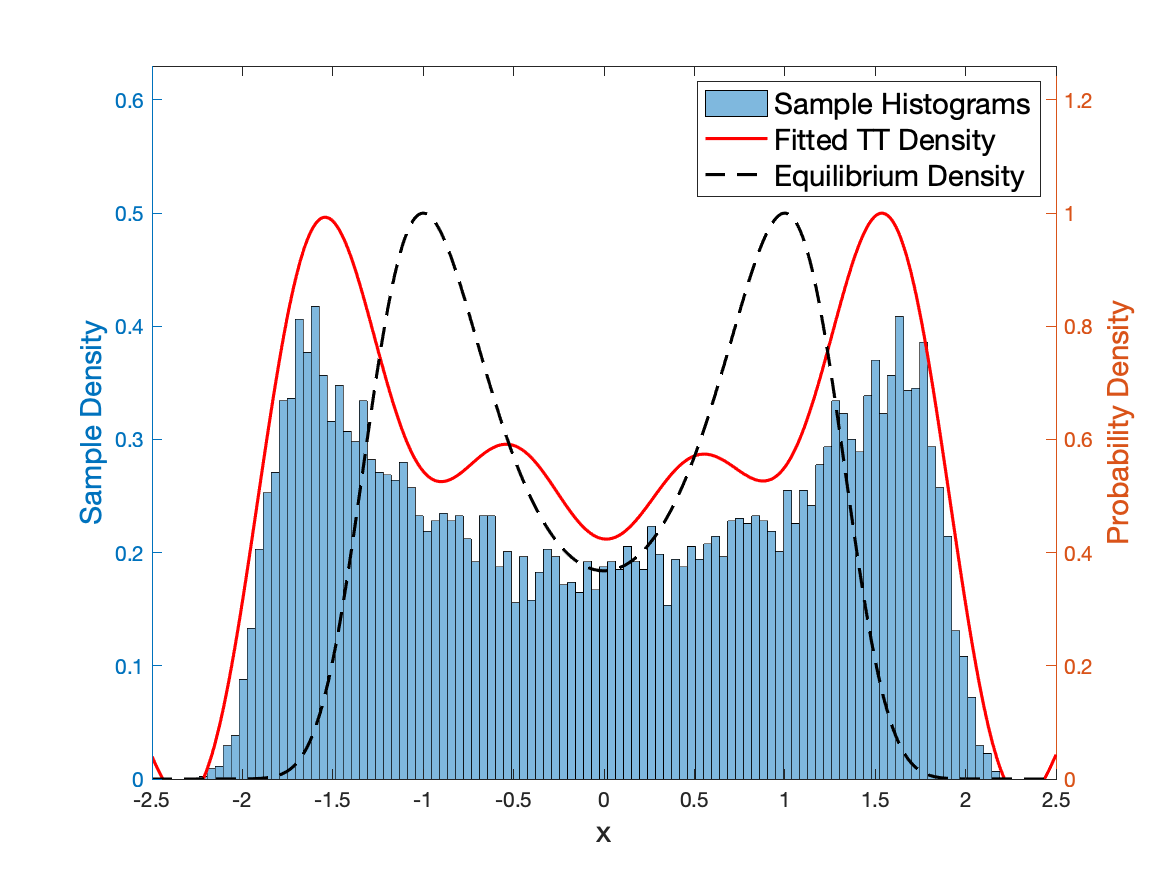
(a) Iteration 1

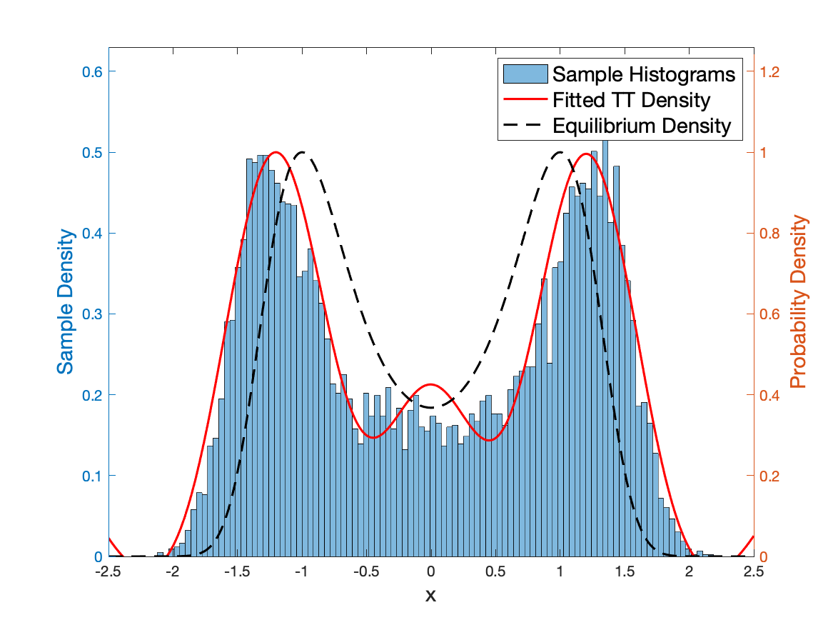
(b) Iteration 3

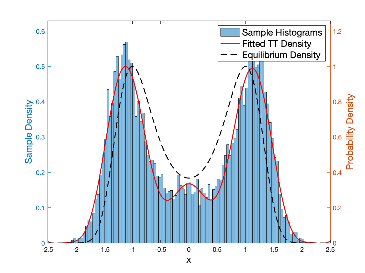
(c) Iteration 5

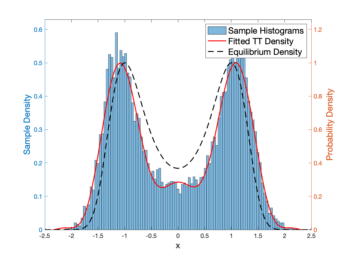
(d) Iteration 7

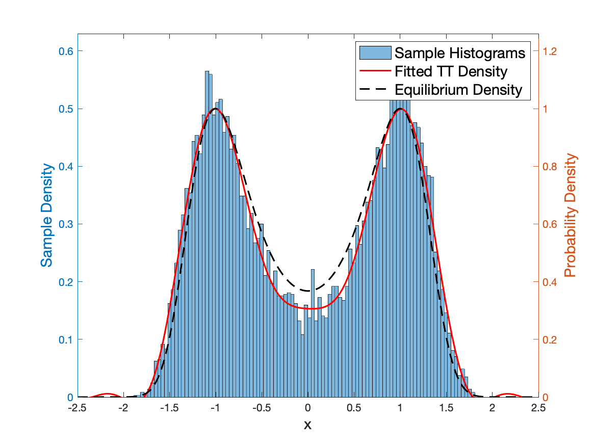
(e) Iteration 20

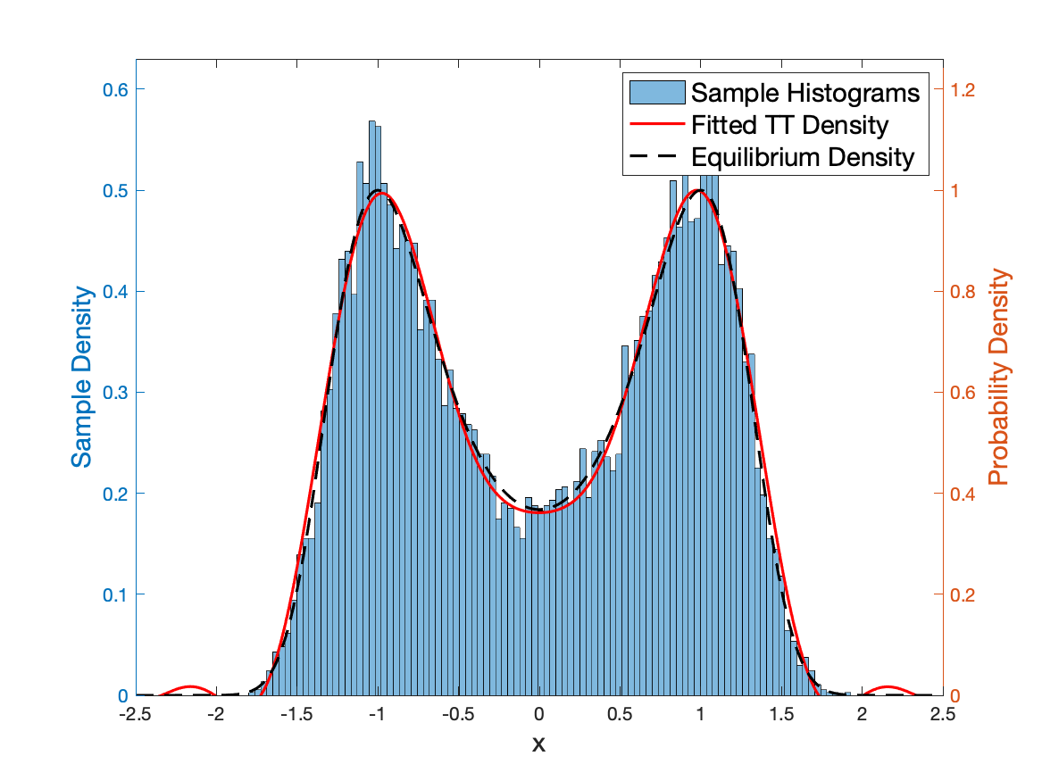
(f) Iteration 30

Figure 6.5. Visualization of the evolution of first marginal for the double-well potential. The blue histograms correspond to the sample histograms after Langevin simulations at each iteration ($\hat{\phi}_{t+1}$ in (3.1)). The estimated continuous MPS/TT density $\hat{\phi}_{\theta_{t+1}}$ in (3.1) and the target equilibrium density $\phi^{*}$ are represented with red solid lines and black dashed lines, respectively.

In Fig. 6.5 we visualize the simulated Langevin particles, the fitted continuous MPS/TT density and the target equilibrium density for the first dimension at iteration $1,3,5,7,20$ and $30$. We can observe that the particle distribution gets evolved effectively by the Langevin dynamics and the fitted continuous MPS/TT density accurately captures the histograms of the particle samples. The low-complexity continuous MPS/TT format also serves as an extra regularization and as a result, is not prone to overfitting. To quantify the performance of our algorithm, we evaluate the relative error metric $E=\|{\phi_{1}}^{*}-{\phi_{1}}_{\theta_{j}}\|/\|{\phi_{1}}^{*}\|$ where ${\phi_{1}}^{*}$ and ${\phi_{1}}_{\theta_{j}}$ are the first marginal distribution of the ground truth and MPS/TT represented distribution, respectively. At iteration $30$, the relative error $E=3.8\times 10^{-2}$. We can further improve the performance of the algorithm by choosing more basis functions and generating more stochastic samples.

6.2.2. 1D Ginzburg-Landau Potential

The Ginzburg-Landau theory was developed to provide a mathematical description of phase transition [GL-model]. In this numerical example, we consider a simplified Ginzburg-Landau model, in which the potential energy is defined as

(6.9) $$V(U):=\sum_{i=1}^{d+1}\frac{\lambda}{2}\left(\frac{U_{i}-U_{i-1}}{h}\right)^{2}+\frac{1}{4\lambda}(1-U_{i}^{2})^{2},$$

where $h=1/(d+1)$, $U_{0}=U_{d+1}=0$. We fix $d=16$, $\lambda=0.03$ and the temperature $\beta=1/8$. We use the same set of $20$ basis function for all dimensions as shown in Fig. 6.4. We use the cluster basis with $c=1,2$ as sketching tensor, which results in a tensor rank $\tilde{r}=240$. For this example, we solve the Fokker-Planck equation starting from the initial uniform distribution over the hypercube $[-M,M]^{d}$ and evolve the distribution with $\delta t=0.002$ time and $N=10^{4}$ samples.

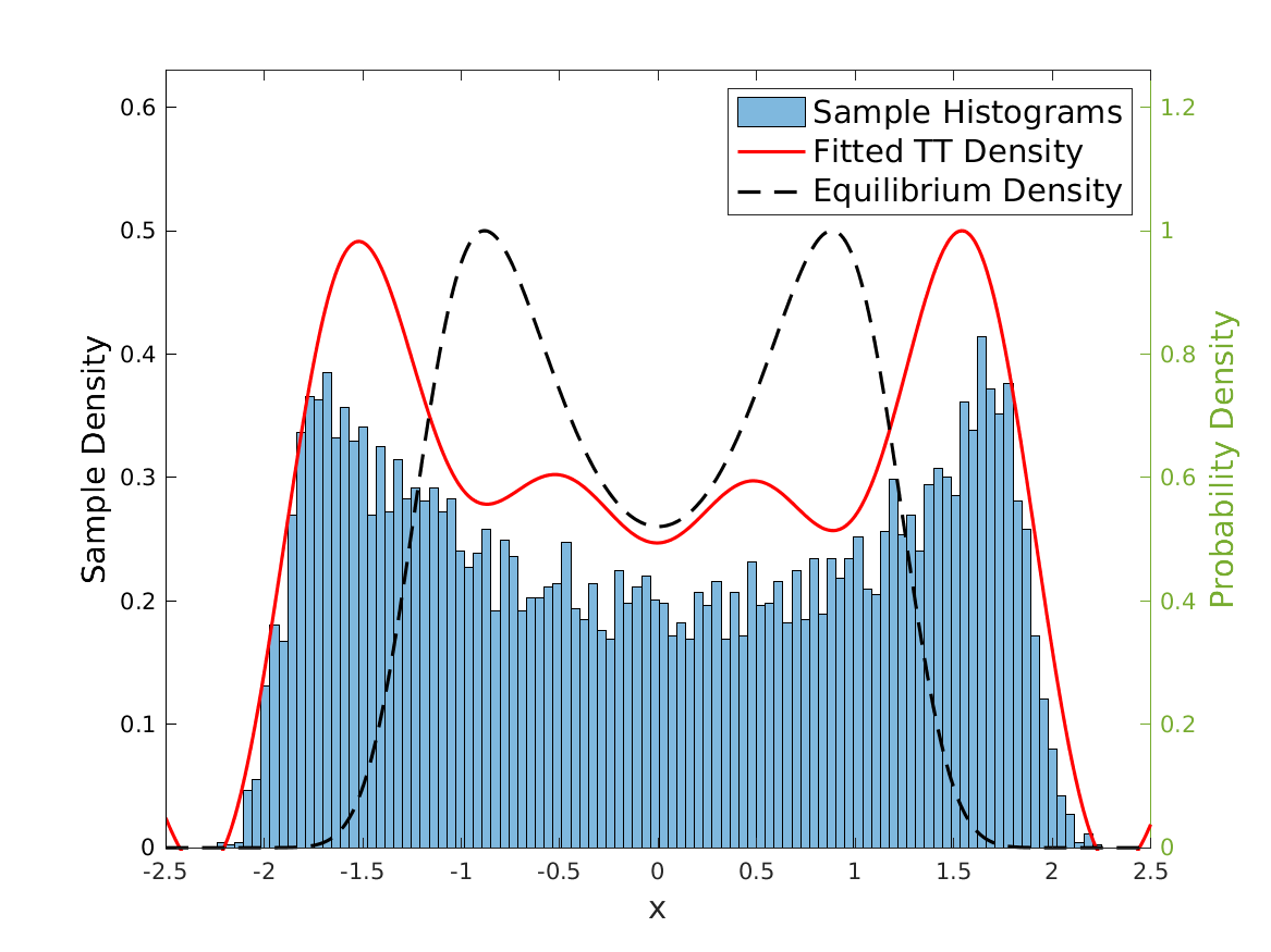
(a) Iteration 1

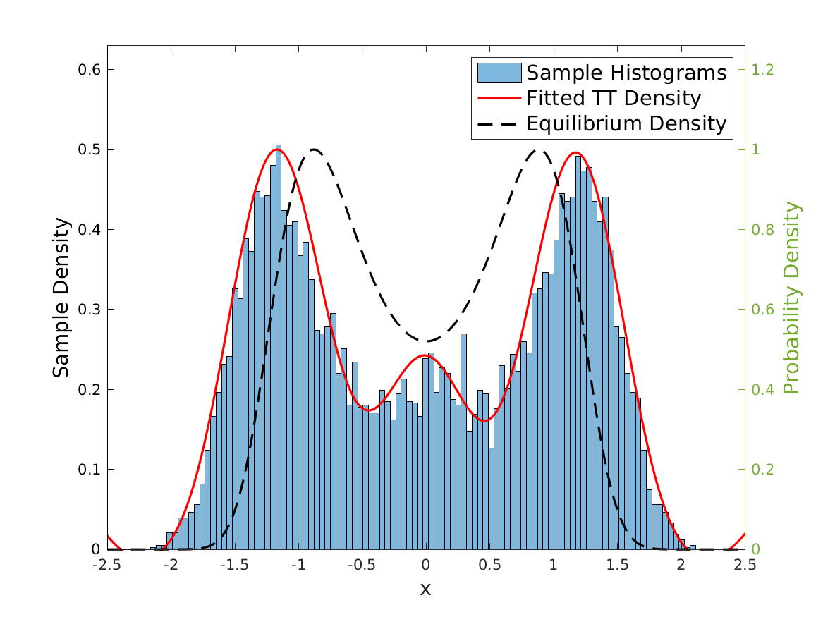
(b) Iteration 3

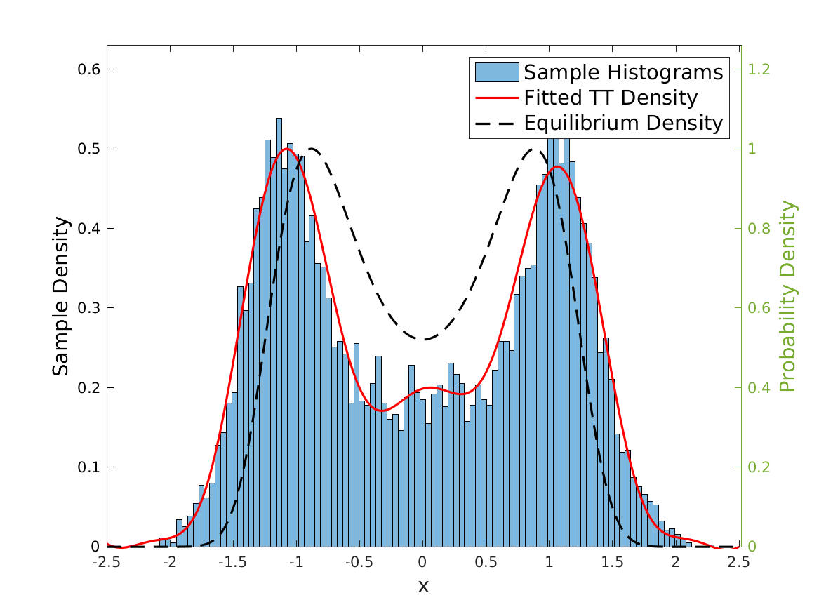
(c) Iteration 5

(d) Iteration 7

(e) Iteration 20

(f) Iteration 100

Figure 6.6. Visualization of the evolution of the 8-th marginal distribution for the 1D Ginzburg-Landau potential. The blue histograms correspond to the sample histograms after Langevin simulations at each iteration ($\hat{\phi}_{t+1}$. in (3.1)) The estimated continuous MPS/TT density $\hat{\phi}_{\theta_{t+1}}$ in (3.1) and the target equilibrium density $\phi^{*}$ are represented with red solid lines and black dashed lines, respectively.

In Fig. 6.6 we visualize the 8-th marginal distribution of the particle dynamics, the MPS/TT density, and the equilibrium density, at iteration $1,3,5,7,20$ and $100$. At iteration $100$, the relative error of the 8-th marginal distribution is $E=9.8\times 10^{-2}$.

6.2.3. 2D Ginzburg-Landau Potential

In this section, we consider an analogous Ginzburg-Landau-type model on a two-dimensional $(\tilde{d}+2,\tilde{d}+2)$ square lattice space. The 2D Ginzburg-Landau example cannot be easily done with the traditional tensor-network method, which requires the compression of the semigroup operator into an MPO. Such a compression is difficult when the variables cannot be ordered along a 1D line. This, however, is not an issue for us, since we never compress any operator in our framework. Similarly, we define the value of the scalar field at lattice points as $U_{i,j}$, $i,j=0,\dots,\tilde{d}+1$, and define the potential energy,

(6.10) $$V(U):=\frac{\lambda}{2}\sum_{i=1}^{\tilde{d}+1}\sum_{j=1}^{\tilde{d}+1}\left[\left(\frac{U_{i,j}-U_{i-1,j}}{h}\right)^{2}+\left(\frac{U_{i,j}-U_{i,j-1}}{h}\right)^{2}\right]+\sum_{i=1}^{\tilde{d}}\sum_{j=1}^{\tilde{d}}\frac{1}{4\lambda}(1-U_{i,j}^{2})^{2},$$

with boundary conditions

(6.11) $$U_{0,:}=U_{\tilde{d}+1,:}=\mathbf{1},\ U_{:,0}=U_{:,\tilde{d}+1}=-\mathbf{1}.$$

Here the total number of dimensionality is $d=\tilde{d}^{2}$. We set $\tilde{d}=4$, $h=1/(d+1)$, $\lambda=0.03$ and the inverse temperature $\beta=1/10$ for this example. All other settings remain the same as in the 1D case (Section 6.2.3). We use the same set of $20$ basis functions for all dimensions as shown in Fig. 6.4 and we use the same cluster basis with $\tilde{r}=240$ as in the previous section. We solve the Fokker-Planck equation starting from the initial uniform distribution over the hypercube $[-M,M]^{d}$ and evolve the distribution with $\delta t=0.002$ time and $N=10^{4}$ samples. To order the dimensions in a 2D lattice into a chain-like structure, we use the $d=16$ space-filling curve (Fig. 6.1).

(a) Iteration 1

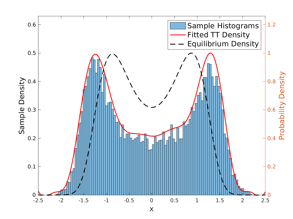
(b) Iteration 3

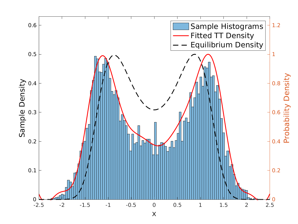
(c) Iteration 5

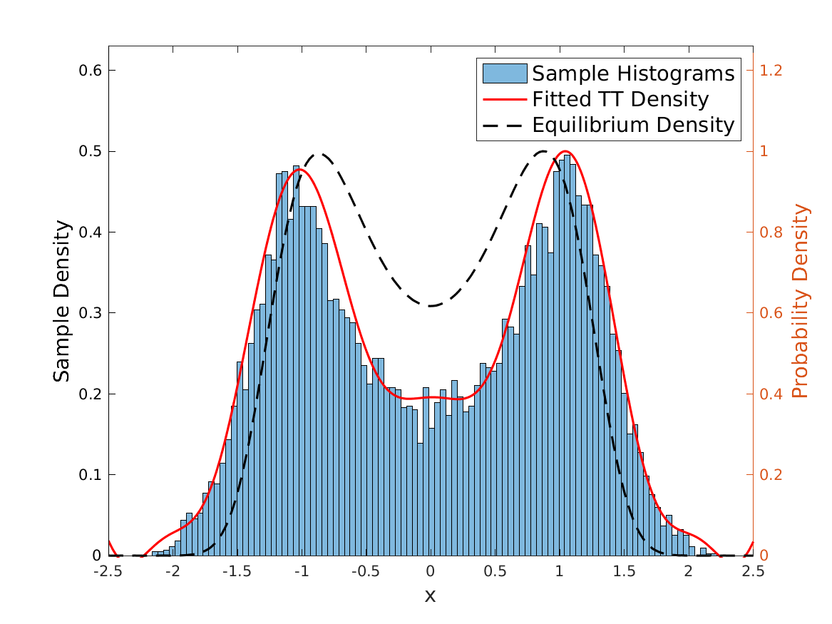
(d) Iteration 7

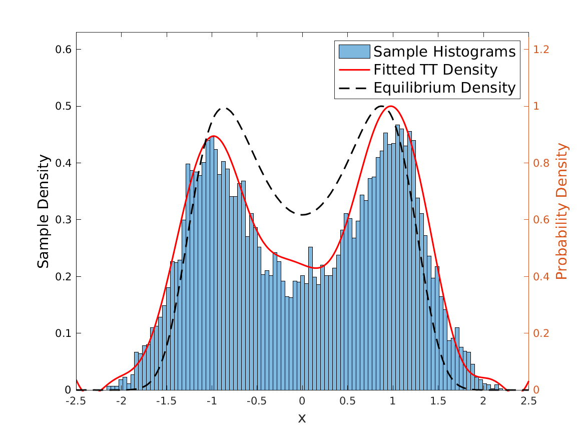
(e) Iteration 20

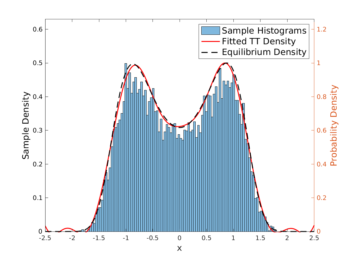
(f) Iteration 100

Figure 6.7. Visualization of the evolution of the 8-th marginal distribution for the 2D Ginzburg-Landau potential. The blue histograms correspond to the sample histograms after Langevin simulations at each iteration ($\hat{\phi}_{t+1}$ in (3.1)). The estimated continuous MPS/TT density $\hat{\phi}_{\theta_{t+1}}$ in (3.1) and the target equilibrium density $\phi^{*}$ are represented with red solid lines and black dashed lines, respectively.

In Fig. 6.7 we visualize the 8-th marginal distribution of the particle dynamics, the MPS/TT density, and the equilibrium density, at iteration $1,3,5,7,20$ and $100$. At iteration $100$, the relative error of the 8-th marginal distribution is $E=2.9\times 10^{-2}$.

7. Conclusion

In this paper, we propose a novel and general framework that combines Monte-Carlo simulation with an MPS/TT ansatz. By leveraging the advantages of both approaches, our method offers an efficient way to apply the semigroup/time-evolution operator and control the variance and population of random walkers using tensor-sketching techniques.

The performance of our algorithm is determined by two factors: the number of randomized sketches and the number of samples used. Our algorithm is expected to succeed when we can employ samples to determine a low-rank MPS/TT representation based on estimating certain low-order moments. Hence, it is crucial to investigate the function space under time evolution and understand how the MPS/TT representation of the solution can be efficiently determined using Monte-Carlo method in a statistically optimal manner.

8. Acknowledgements

Y.C. and Y.K. acknowledge partial support from NSF Award No. DMS-211563 and DOE Award No. DE-SC0022232. The authors also thank Michael Lindsey and Shiwei Zhang regarding discussions on potential improvements for the proposed method.