Fractal uncertainty in higher dimensions:
notes on Cohen’s paper

Abstract.

In [Coh23], Cohen proved a higher dimensional fractal uncertainty principle for line porous sets. The purpose of this expository note is to provide a different point of view on some parts of Cohen’s proof, particularly suited to readers familiar with the theory of distributions. It is meant to be complementary to Cohen’s paper.

In the recent paper [Coh23, Theorem 1.2], Cohen proved the following remarkable

Theorem 1.

Assume that $\mathbf{X},\mathbf{Y}\subset\mathbb{R}^{d}$ are two sets such that for some $h\in(0,{1\over 100})$ and $\nu\in(0,{1\over 10})$

• $\mathbf{X}\subset B(0,1)$ is $\nu$-porous on balls on scales $h$ to 1, and

• $\mathbf{Y}\subset B(0,h^{-1})$ is $\nu$-porous on lines on scales 1 to $h^{-1}$.

Then we have the following estimate for all $f\in L^{2}(\mathbb{R}^{d})$

$$\operatorname{supp}\widehat{f}\subset\mathbf{Y}\quad\Longrightarrow\quad\|\operatorname{1\hskip-2.75ptl}_{\mathbf{X}}f\|_{L^{2}(\mathbb{R}^{d})}\leq Ch^{\beta}\|f\|_{L^{2}(\mathbb{R}^{d})}$$ (1.1)

where the constants $C,\beta>0$ depend only on $\nu,d$ but not on $h$.

Here $B(\mathbf{x},r)$ denotes the $r$-ball centered at $\mathbf{x}$ and the notion of porosity is given by

Definition 1.1.

Assume that $0<\rho_{0}\leq\rho_{1}$, $\nu\in(0,{1\over 10})$, and $\mathbf{X}\subset\mathbb{R}^{d}$.

• We say that $\mathbf{X}$ is $\nu$-porous on balls on scales $\rho_{0}$ to $\rho_{1}$ if for each ball $B$ of diameter $R\in[\rho_{0},\rho_{1}]$ there exists $\mathbf{x}\in B$ such that $\mathbf{X}\cap B(\mathbf{x},\nu R)=\emptyset$.

• We say that $\mathbf{X}$ is $\nu$-porous on lines on scales $\rho_{0}$ to $\rho_{1}$ if for each line segment $\tau$ of length $R\in[\rho_{0},\rho_{1}]$ there exists $\mathbf{x}\in\tau$ such that $\mathbf{X}\cap B(\mathbf{x},\nu R)=\emptyset$.

Note that porosity on lines implies porosity on balls but the converse is not true when $d\geq 2$: any line in $\mathbb{R}^{d}$ is $\frac{1}{10}$-porous on balls on all scales but not porous on lines.

Our statement of Theorem 1 (as well as the statements of various results below) differs from the one in [Coh23] in minor details, in particular we use the following normalization of the Fourier transform following [Hör03]:

$$\widehat{f}(\xi)=\int_{\mathbb{R}^{d}}e^{-i\mathbf{x}\cdot\xi}f(\mathbf{x})\,d\mathbf{x}.$$

This expository note gives a different point of view on some parts of Cohen’s proof of Theorem 1. We will freely use the theory of distributions presented for example in [Hör03], which is not necessary (as it is not used in [Coh23]) but is convenient in particular because of the distributional characterization of plurisubharmonicity (Proposition 2.6 below).

This note is meant to be complementary to Cohen’s paper and in particular contains no discussion of applications of fractal uncertainty principle or previous results; the latter can be found for instance in [Dya19]. We also only present the proof of a part of the argument, namely Theorems 3 and 5 below (it is possible that a future version of this note will contain other parts as well).

We restrict to the case of dimension $d=2$. This is only for the purpose of notational convenience, shortening various formulas along the way. For the case of dimension $d=1$, Theorem 1 was proved by Bourgain–Dyatlov [BD18] and Cohen’s result [Coh23] is a far-reaching generalization of this result to all dimensions.

1.1. Existence of special compactly supported functions

Theorem 1 is deduced in [Coh23] from the result of Han–Schlag [HS20] and a novel construction of compactly supported functions with Fourier transforms decaying on line porous sets [Coh23, Proposition 1.7]. We state a slightly weaker version of the latter construction as Theorem 2 below. (Comparing to [BD18], the paper [HS20] generalizes [BD18, §§3.2–3.4] and Theorem 2 generalizes [BD18, Lemma 3.1].) We denote $\langle\mathbf{x}\rangle:=\sqrt{1+|\mathbf{x}|^{2}}$.

Theorem 2.

Assume that $\mathbf{Y}\subset B(0,h^{-1})$ is $\nu$-porous on lines on scales 1 to $h^{-1}$. Then for each $c_{\operatorname{supp}}>0$ there exist $c_{2},c_{3}>0$ and $\alpha\in(0,1)$ depending only on $\nu,c_{\operatorname{supp}}$ and there exists a function $g\in L^{2}(\mathbb{R}^{2})$ satisfying the following conditions:

$$\operatorname{supp}\widehat{g} \subset B(0,c_{\operatorname{supp}}),$$ (1.2)

$$\|g\|_{L^{2}(B(0,1))} \geq c_{2},$$ (1.3)

$$|g(\mathbf{x})| \leq 1\quad\text{for all }\mathbf{x}\in\mathbb{R}^{2},$$ (1.4)

$$|g(\mathbf{x})| \leq\exp\bigg{(}-c_{3}{|\mathbf{x}|\over(\log|\mathbf{x}|)^{\alpha}}\bigg{)}\quad\text{ for all }\mathbf{x}\in\mathbf{Y}\setminus B(0,10).$$ (1.5)

We note that for $\alpha>1$, one can construct a function satisfying conditions (1.2)–(1.5) with $\mathbf{Y}=\mathbb{R}^{2}$. However, this is impossible for $\alpha<1$, in fact if $g$ satisfies the condition (1.5) on the entire $\mathbb{R}^{2}$ then $\widehat{g}$ satisfies a unique continuation principle and thus cannot be compactly supported. The argument of [HS20] uses this unique continuation principle and induction on scales to show that Theorem 2 implies Theorem 1.

In [BD18], the analog of Theorem 2 in the case of dimension $d=1$ was proved by constructing a weight $\omega\leq 0$ which behaves like $-|x|/(\log|x|)^{\alpha}$ for $x\in\mathbf{Y}\setminus B(0,10)$ but also satisfies $\int_{\mathbb{R}}\langle x\rangle^{-2}\omega(x)\,dx>-\infty$; this was possible due to the porosity of $\mathbf{Y}$. Then one used the Beurling–Malliavin Theorem to construct a function $g$ satisfying (1.2)–(1.4) and $|g|\leq\exp(c_{3}\omega)$, which implies (1.5).

In [Coh23] Cohen also constructs a weight $\omega$ with the right kind of behavior on $\mathbf{Y}$ (stated as Theorem 3 below) and satisfying the right conditions so that one can construct a function $g$ satisfying (1.2)–(1.4) and $|g|\leq\exp(c_{3}\omega)$ (stated as Theorem 4 below). We now describe these ‘right conditions’, or rather their slight modification making the split into dyadic pieces explicit. For that we need a few definitions:

• Define the Kohn–Nirenberg symbolic norm of order 1 with 3 derivatives on the space of smooth compactly supported functions $C^{\infty}_{\mathrm{c}}(\mathbb{R}^{2})$ as follows:

  $$\|\psi\|_{S^{1}_{3}}:=\max_{|\gamma|\leq 3}\sup_{\mathbf{x}\in\mathbb{R}^{2}}|\langle\mathbf{x}\rangle^{|\gamma|-1}\partial_{\mathbf{x}}^{\gamma}\psi(\mathbf{x})|.$$ (1.6)

• For a function $\psi\in C^{\infty}_{\mathrm{c}}(\mathbb{R}^{2})$, define its X-ray transform as the function $T\psi\in C^{\infty}_{\mathrm{c}}(\mathbb{R}_{s}\times\mathbb{S}^{1}_{\theta})$, where $\mathbb{S}^{1}=\mathbb{R}/2\pi\mathbb{Z}$, given by the formula

  $$T\psi(s,\theta):=\int_{\mathbb{R}}\psi(t\cos\theta-s\sin\theta,t\sin\theta+s\cos\theta)\,dt.$$ (1.7)

  Note that $T\psi(s,\theta)$ is the integral of $\psi$ over a line in the direction given by the angle $\theta$ which is distance $|s|$ from the origin – see Figure 1. In particular, $T\psi(0,\theta)$ is the integral of $\psi$ over a line passing through the origin.

Figure 1. An illustration of the X-ray transform: $T\psi(s,\theta)$ is the integral of $\psi$ over the thick line.

The weight $\omega$ will have the form

$$\omega=\sum_{k\geq 1}\omega_{k}\quad\text{where }\omega_{k}\in C^{\infty}_{\mathrm{c}}(\mathbb{R}^{2};(-\infty,0]),\quad k\in\mathbb{N}.$$ (1.8)

Here the summands $\omega_{k}$ satisfy the following conditions for some constants $C_{\mathrm{reg}},C_{\mathrm{gr}}\geq 0$:

$$\omega_{k} =0\quad\text{for $k$ large enough},$$ (1.9)

$$\operatorname{supp}\omega_{k} \subset\{2^{k-1}\leq|\mathbf{x}|\leq 2^{k+1}\},$$ (1.10)

$$\|\omega_{k}\|_{S^{1}_{3}} \leq C_{\mathrm{reg}},$$ (1.11)

$$\sum_{k=1}^{\infty}q_{k} \leq C_{\mathrm{gr}}\quad\text{where }q_{k}:=-\inf_{\theta\in\mathbb{S}^{1}}T(|\mathbf{x}|^{-2}\omega_{k})(0,\theta).$$ (1.12)

We give a few comments on the above conditions:

• (1.9) ensures that $\omega\in C^{\infty}_{\mathrm{c}}(\mathbb{R}^{2})$. It is made for technical convenience. Note that the constants in the results below do not depend on how many of the functions $\omega_{k}$ are nonzero.

• (1.10) requires that each $\omega_{k}$ is supported in a dyadic annulus.

• (1.11) is a Kohn–Nirenberg type regularity condition on each $\omega_{k}$, in particular ensuring that the total weight $\omega$ is bounded in $S^{1}_{3}$. Given (1.10), we can rewrite it in the following form:

  $$\sup|\partial^{\gamma}_{\mathbf{x}}\omega_{k}|\leq\widetilde{C}_{\mathrm{reg}}2^{(1-|\gamma|)k}\quad\text{for }|\gamma|\leq 3.$$ (1.13)

• (1.12) is a condition on the growth of $\omega_{k}$ along lines passing through the origin. It implies in particular that $T(|\mathbf{x}|^{-2}\omega)(0,\theta)\geq-C_{\mathrm{gr}}$ for all $\theta$ but it is stronger due to the infimum in the definition of $q_{k}$. Note also that each $q_{k}$ is bounded in terms of the regularity constant $C_{\mathrm{reg}}$ alone, more precisely we have

  $$0\leq q_{k}\leq 10C_{\mathrm{reg}}.$$ (1.14)

  The role of the growth constant $C_{\mathrm{gr}}$ is to control the sum of $q_{k}$ over the dyadic scales.

We now state two theorems which together give Theorem 2. The first one (similar to the result of [Coh23, §6.1] and proved in §3 below) is the existence of a weight satisfying the above conditions and also sufficiently negative on a line porous set:

Theorem 3.

Assume that $\mathbf{Y}\subset B(0,h^{-1})$ is $\nu$-porous on lines on scales $1$ to $h^{-1}$. Then there exists a weight $\omega$ of the form (1.8) such that:

• the summands $\omega_{k}$ satisfy the conditions (1.9)–(1.12) for some constants $C_{\mathrm{reg}},C_{\mathrm{gr}}$ depending only on the porosity constant $\nu$, and

• there exists $\alpha\in(0,1)$ depending only on $\nu$ such that

  $$\omega(\mathbf{x})\leq-{|\mathbf{x}|\over(\log|\mathbf{x}|)^{\alpha}}\quad\text{for all }\mathbf{x}\in\mathbf{Y}\setminus B(0,10).$$ (1.15)

The second one, which is perhaps the main novelty of Cohen’s paper and is a result of independent interest, is the following higher dimensional version of the Beurling–Malliavin Theorem, see [Coh23, Theorem 1.4]:

Theorem 4.

Assume that $\omega$ is given by (1.8) where $\omega_{k}$ satisfy the conditions (1.9)–(1.12) for some constants $C_{\mathrm{reg}},C_{\mathrm{gr}}$. Fix also $c_{\operatorname{supp}}>0$. Then there exist $c_{2},c_{3}>0$ depending only on $C_{\mathrm{reg}},C_{\mathrm{gr}},c_{\operatorname{supp}}$ and there exists $g\in L^{2}(\mathbb{R}^{2})$ which satisfies the conditions (1.2)–(1.3) and

$$|g(\mathbf{x})|\leq\exp(c_{3}\omega(\mathbf{x}))\quad\text{for all }\mathbf{x}\in\mathbb{R}^{2}.$$ (1.16)

We note that the analog of Theorem 4 in dimension $d=1$ is weaker than the Beurling–Malliavin Theorem due to the regularity assumption (1.11), but it suffices for the purposes of proving a Fractal Uncertainty Principle as shown by Theorem 3.

1.2. Constructing plurisubharmonic functions on $\mathbb{C}^{2}$

We now discuss the proof of Theorem 4. By the Paley–Wiener Theorem, the compact Fourier support condition (1.2) is essentially equivalent to the function $g$ having a holomorphic extension $G:\mathbb{C}^{2}\to\mathbb{C}$ which satisfies the bound for some $C\geq 0$

$$\log|G(\mathbf{x}+i\mathbf{y})|\leq c_{\operatorname{supp}}|\mathbf{y}|+C\quad\text{for all }\mathbf{x},\mathbf{y}\in\mathbb{R}^{2}.$$ (1.17)

In terms of the function $G$, the condition (1.16) becomes

$$\log|G(\mathbf{x})|\leq c_{3}\omega(\mathbf{x})\quad\text{for all }\mathbf{x}\in\mathbb{R}^{2}.$$ (1.18)

Note that (1.18) is stronger than (1.17) on $\mathbb{R}^{2}$ (since $\omega\leq 0$) but (1.17) needs to hold on the entire $\mathbb{C}^{2}$.

Since $G$ is holomorphic, the function $\log|G|$ is plurisubharmonic on $\mathbb{C}^{2}$. Thus the existence of a nonzero function $g$ satisfying (1.2) and (1.16) implies that there exists a plurisubharmonic function $\widetilde{u}:\mathbb{C}^{2}\to[-\infty,\infty)$ satisfying

$$\widetilde{u}(\mathbf{x}+i\mathbf{y}) \leq c_{3}^{-1}c_{\operatorname{supp}}|\mathbf{y}|\quad\text{for all }\mathbf{x},\mathbf{y}\in\mathbb{R}^{2},$$ (1.19)

$$\widetilde{u}(\mathbf{x}) \leq\omega(\mathbf{x})\quad\text{for all }\mathbf{x}\in\mathbb{R}^{2}.$$ (1.20)

Namely, one can take $\widetilde{u}:=c_{3}^{-1}(\log|G|-C)$.

Following an unpublished note by Bourgain, Cohen uses Hörmander’s $\bar{\partial}$-theorem to show the converse statement: starting from a plurisubharmonic function $\widetilde{u}$ satisfying the bounds (1.19)–(1.20) one can construct a holomorphic function $G$ satisfying (1.17)–(1.18) and obtain Theorem 4. This is described in [Coh23, §5] and we do not give the details here (hopefully this part of the argument will be in the next version of this note).

Thus Theorem 4 is reduced to constructing a plurisubharmonic function $\widetilde{u}$ satisfying (1.19)–(1.20). To do the latter, Cohen introduces the extension operator

$$E:C^{\infty}_{\mathrm{c}}(\mathbb{R}^{2})\to C^{0}(\mathbb{C}^{2})$$ (1.21)

defined as follows: for $\omega\in C^{\infty}_{\mathrm{c}}(\mathbb{R}^{2})$,

$$E\omega(\mathbf{x}+i\mathbf{y}):={1\over\pi}\int_{\mathbb{R}}{\omega(\mathbf{x}+t\mathbf{y})\over 1+t^{2}}\,dt,\quad\mathbf{x},\mathbf{y}\in\mathbb{R}^{2}.$$ (1.22)

Here continuity of $E\omega$ follows from the Dominated Convergence Theorem; in fact, differentiating under the integral sign, we also have $E\omega\in C^{\infty}(\mathbb{C}^{2}\setminus\mathbb{R}^{2})$. Moreover, $E\omega$ is an extension of $\omega$, namely

$$E\omega(\mathbf{x})=\omega(\mathbf{x})\quad\text{for all }\mathbf{x}\in\mathbb{R}^{2}.$$ (1.23)

Now, the needed function $\widetilde{u}$ will have the form

$$\widetilde{u}(\mathbf{x}+i\mathbf{y}):=E\widetilde{\omega}(\mathbf{x}+i\mathbf{y})+\sigma|\mathbf{y}|,\quad\mathbf{x},\mathbf{y}\in\mathbb{R}^{2}$$ (1.24)

where $\widetilde{\omega}\in C^{\infty}_{\mathrm{c}}(\mathbb{R}^{2})$ is an auxiliary weight which satisfies $\widetilde{\omega}\leq\omega\leq 0$ and $\sigma\geq 0$ is a constant. We have $E\widetilde{\omega}\leq 0$, so $\widetilde{u}$ satisfies (1.19) if we put $c_{3}:=c_{\operatorname{supp}}/\sigma$. It also satisfies (1.20) as follows from (1.23).

Thus we need to show that when the weight $\omega$ satisfies the conditions of Theorem 4 and $\sigma$ is large enough, the function $\widetilde{u}$ is plurisubharmonic. This is done in the following

Theorem 5.

Assume that $\omega$ is given by (1.8) where $\omega_{k}$ satisfy the conditions (1.9)–(1.12) for some constants $C_{\mathrm{reg}},C_{\mathrm{gr}}$. Then there exists $\widetilde{\omega}\in C^{\infty}_{\mathrm{c}}(\mathbb{R}^{2})$ such that $\widetilde{\omega}\leq\omega$ everywhere and for $\sigma\geq 0$ large enough depending only on $C_{\mathrm{reg}},C_{\mathrm{gr}}$ the function $\widetilde{u}$ defined by (1.24) is plurisubharmonic on $\mathbb{C}^{2}$.

The proof of Theorem 5 is presented in this note in §§4–5. It largely follows Cohen’s original proof in [Coh23], with a few changes:

• we specialize to the case of dimension 2;

• we use the distributional criterion for plurisubharmonicity, which eliminates Cohen’s condition on Hilbert transforms on lines (see Remark 4.2 below);

• we explicitly write the weight $\omega$ as a dyadic sum (1.8), which makes the conditions of Theorem 5 more complicated but shortens the proof a bit, and is acceptable for applications to FUP since the weight in Theorem 3 is constructed as a dyadic sum as well.

2. Preliminaries

2.1. X-ray transform

We first state several basic properties of the X-ray transform defined in (1.7). Throughout this section we assume that $\psi\in C^{\infty}_{\mathrm{c}}(\mathbb{R}^{2})$. First of all, we have the discrete symmetry

$$T\psi(-s,\theta)=T\psi(s,\theta+\pi).$$ (2.1)

We also have equivariance under rotations: if $\mathcal{R}_{\gamma}:\mathbb{R}^{2}\to\mathbb{R}^{2}$ is the linear map given by

$$\mathcal{R}_{\gamma}(x_{1},x_{2})=(x_{1}\cos\gamma-x_{2}\sin\gamma,x_{1}\sin\gamma+x_{2}\cos\gamma)$$ (2.2)

then we have

$$T(\psi\circ\mathcal{R}_{\gamma})(s,\theta)=T\psi(s,\theta+\gamma).$$ (2.3)

We next prove two identities featuring the X-ray transform and the Laplace operator $\Delta=\partial_{x_{1}}^{2}+\partial_{x_{2}}^{2}$ on $\mathbb{R}^{2}$. First of all, for $\gamma\in\mathbb{S}^{1}$ define the constant vector field on $\mathbb{R}^{2}$

$$V_{\gamma}:=(\cos\gamma)\partial_{x_{1}}+(\sin\gamma)\partial_{x_{2}}.$$

We treat $V_{\gamma}$ as a first order differential operator.

Our first identity is used in §4.3.

Lemma 2.1.

We have for all $\gamma\in\mathbb{S}^{1}$

$$T(V_{\gamma}^{2}\psi)(s,\theta)=\sin^{2}(\theta-\gamma)T(\Delta\psi)(s,\theta).$$ (2.4)

Proof.

By the rotational equivariance (2.3) and the identity $(V_{\gamma}\psi)\circ R_{\theta}=V_{\gamma-\theta}(\psi\circ R_{\theta})$ it suffices to consider the case $\theta=0$. Integrating by parts in $x_{1}$ and using the fact that $\psi$ is compactly supported, we get

$$T(V_{\gamma}^{2}\psi)(s,0) =\int_{\mathbb{R}}V_{\gamma}^{2}\psi(x_{1},s)\,dx_{1}=\sin^{2}\gamma\int_{\mathbb{R}}\partial_{x_{2}}^{2}\psi(x_{1},s)\,dx_{1},$$ (2.5)

$$T(\Delta\psi)(s,0) =\int_{\mathbb{R}}\Delta\psi(x_{1},s)\,dx_{1}=\int_{\mathbb{R}}\partial_{x_{2}}^{2}\psi(x_{1},s)\,dx_{1}$$ (2.6)

which together give (2.4). ∎

The next identity is used in §5.1.

Lemma 2.2.

Assume that $\psi\in C^{\infty}_{\mathrm{c}}(\mathbb{R}^{2}\setminus\{0\})$. Then we have for all $\theta\in\mathbb{S}^{1}$

$$T(\Delta\psi)(0,\theta)=(\partial_{\theta}^{2}+1)T(|\mathbf{x}|^{-2}\psi)(0,\theta).$$ (2.7)

Proof.

By rotational equivariance (2.3) it suffices to show (2.7) when $\theta=0$. For all $\theta\in\mathbb{S}^{1}$ we have

$$T(|\mathbf{x}|^{-2}\psi)(0,\theta)=\int_{\mathbb{R}}t^{-2}\psi(t\cos\theta,t\sin\theta)\,dt.$$

Differentiating this twice at $\theta=0$ we get

$$(\partial_{\theta}^{2}+1)T(|\mathbf{x}|^{-2}\psi)(0,0) =\int_{\mathbb{R}}\partial_{x_{2}}^{2}\psi(t,0)-t^{-1}\partial_{x_{1}}\psi(t,0)+t^{-2}\psi(t,0)\,dt$$

$$=\int_{\mathbb{R}}(\Delta\psi)(t,0)\,dt=T(\Delta\psi)(0,0)$$

where in the last line we used that

$$\int_{\mathbb{R}}\partial_{t}\big{(}\partial_{x_{1}}\psi(t,0)+t^{-1}\psi(t,0)\big{)}\,dt=0.$$

∎

2.2. X-ray transform and Hilbert transform

We next explain how the X-ray transform is related to the Hilbert transform. This is only used in Remark 4.2 rather than in the main proof.

The Hilbert transform is defined as the following convolution:

$$\mathcal{H}:C^{\infty}_{\mathrm{c}}(\mathbb{R})\to C^{\infty}(\mathbb{R})\cap L^{\infty}(\mathbb{R}),\quad\mathcal{H}f={1\over\pi}\Big{(}\mathrm{p.v.}{1\over x}\Big{)}*f$$

where the principal value distribution $\mathrm{p.v.}{1\over x}\in\mathscr{S}^{\prime}(\mathbb{R})$ is the (distributional) derivative of $\log|x|\in L^{1}_{\operatorname{loc}}(\mathbb{R})$. Denote by $\mathcal{H}f^{\prime}$ the derivative of $\mathcal{H}f$.

We show that if $\psi\in C^{\infty}_{\mathrm{c}}(\mathbb{R}^{2})$ and $\ell$ is a line in $\mathbb{R}^{2}$ passing through a point $\mathbf{x}_{0}$, then the Hilbert transform of the restriction $\psi|_{\ell}$ at $\mathbf{x}_{0}$ can be expressed as a weighted integral of the X-ray transform $T(\Delta\psi)$ over the lines passing through $\mathbf{x}_{0}$. For simplicity we restrict to the case when $\mathbf{x}_{0}=0$ and the line $\ell$ is horizontal:

Lemma 2.3.

Let $\psi\in C^{\infty}_{\mathrm{c}}(\mathbb{R}^{2})$ and $\varphi\in C^{\infty}_{\mathrm{c}}(\mathbb{R})$ be defined by $\varphi(x_{1}):=\psi(x_{1},0)$. Then

$$\mathcal{H}\varphi^{\prime}(0)=-{1\over 4\pi}\int_{\mathbb{S}^{1}}|\sin\theta|\,T(\Delta\psi)(0,\theta)\,d\theta.$$ (2.8)

Remark 2.4.

In case $\operatorname{supp}\psi\subset\mathbb{R}^{2}\setminus\{0\}$, (2.8) follows from (2.7), integration by parts in $\theta$, and (2.1) since $(\partial_{\theta}^{2}+1)|\sin\theta|=2(\delta(\theta)+\delta(\theta-\pi))$ and

$$\mathcal{H}\varphi^{\prime}(0)=-{1\over\pi}\int_{\mathbb{R}}x_{1}^{-2}\psi(x_{1},0)\,dx_{1}=-{1\over\pi}T(|\mathbf{x}|^{-2}\psi)(0,0).$$

Proof.

We express both sides of (2.8) in terms of the Fourier transform $\widehat{\psi}$.

1. First of all, by the Fourier Inversion Formula we have

$$\widehat{\varphi}(\xi_{1})={1\over 2\pi}\int_{\mathbb{R}}\widehat{\psi}(\xi_{1},\xi_{2})\,d\xi_{2}.$$

The Hilbert transform is a Fourier multiplier, more precisely

$$\widehat{\mathcal{H}\varphi}(\xi_{1})=-i(\operatorname{sgn}\xi_{1})\widehat{\varphi}(\xi_{1}).$$

Using the Fourier Inversion Formula again, we get a formula for the left-hand side of (2.8):

$$\mathcal{H}\varphi^{\prime}(0) ={1\over 2\pi}\int_{\mathbb{R}}\widehat{\mathcal{H}\varphi^{\prime}}(\xi_{1})\,d\xi_{1}={1\over 2\pi}\int_{\mathbb{R}}|\xi_{1}|\,\widehat{\varphi}(\xi_{1})\,d\xi_{1}$$ (2.9)

$$={1\over 4\pi^{2}}\int_{\mathbb{R}^{2}}|\xi_{1}|\,\widehat{\psi}(\xi_{1},\xi_{2})\,d\xi_{1}d\xi_{2}.$$

2. For a fixed $\theta\in\mathbb{S}^{1}$, the Fourier transform of $T(\Delta\psi)$ in the $s$ variable is given by

$$\int_{\mathbb{R}}e^{-i\eta s}T(\Delta\psi)(s,\theta)\,ds =\int_{\mathbb{R}^{2}}e^{-i\eta s}\Delta\psi(t\cos\theta-s\sin\theta,t\sin\theta+s\cos\theta)\,dtds$$

$$=\int_{\mathbb{R}^{2}}e^{-i\eta(x_{2}\cos\theta-x_{1}\sin\theta)}\Delta\psi(x_{1},x_{2})\,dx_{1}dx_{2}$$

$$=-\eta^{2}\widehat{\psi}(-\eta\sin\theta,\eta\cos\theta).$$

Here in the second line we make the linear change of variables $(x_{1},x_{2})=\mathcal{R}_{\theta}(t,s)$ where $\mathcal{R}_{\theta}$ is the rotation defined in (2.2).

By the Fourier Inversion Formula, we get the following expression of the X-ray transform $T(\Delta\psi)(0,\theta)$ in terms of the Fourier transform of $\psi$:

$$T(\Delta\psi)(0,\theta)=-{1\over 2\pi}\int_{\mathbb{R}}\eta^{2}\,\widehat{\psi}(-\eta\sin\theta,\eta\cos\theta)\,d\eta.$$ (2.10)

3. We now write the integral (2.9) in polar coordinates $(\xi_{1},\xi_{2})=(-\eta\sin\theta,\eta\cos\theta)$:

$$\mathcal{H}\varphi^{\prime}(0) ={1\over 4\pi^{2}}\int_{0}^{\infty}\eta^{2}\int_{\mathbb{S}^{1}}|\sin\theta|\,\widehat{\psi}(-\eta\sin\theta,\eta\cos\theta)\,d\theta d\eta$$

$$={1\over 8\pi^{2}}\int_{\mathbb{R}\times\mathbb{S}^{1}}\eta^{2}|\sin\theta|\,\widehat{\psi}(-\eta\sin\theta,\eta\cos\theta)\,d\theta d\eta$$

$$=-{1\over 4\pi}\int_{\mathbb{S}^{1}}|\sin\theta|\,T(\Delta\psi)(0,\theta)\,d\theta$$

which gives (2.8). Here in the second line we use that the inner integral $d\theta$ is an even function of $\eta\in\mathbb{R}$ and in the last line we use (2.10). ∎

2.3. Plurisubharmonic functions

We review the concept of plurisubharmonicity on $\mathbb{C}^{2}$. We first give the classical definition:

Definition 2.5.

Let $u:\mathbb{C}^{2}\to[-\infty,\infty)$ be an upper semicontinuous function not identically equal to $-\infty$. We say $u$ is plurisubharmonic if for each $\mathbf{z},\mathbf{v}\in\mathbb{C}^{2}$ we have the sub-mean value property

$$u(\mathbf{z})\leq{1\over 2\pi}\int_{\mathbb{S}^{1}}u(\mathbf{z}+e^{i\theta}\mathbf{v})\,d\theta.$$ (2.11)

In this paper we will instead use the alternative definition in terms of partial derivatives defined using the operators (where we write points in $\mathbb{C}^{2}$ as $\mathbf{z}=(x_{1}+iy_{1},x_{2}+iy_{2})$)

$$\partial_{z_{j}}=\tfrac{1}{2}(\partial_{x_{j}}-i\partial_{y_{j}}),\quad\partial_{\bar{z}_{j}}=\tfrac{1}{2}(\partial_{x_{j}}+i\partial_{y_{j}}).$$

For $u\in C^{2}(\mathbb{C}^{2};\mathbb{R})$ we define the Hermitian matrix

$$\partial_{\bar{\mathbf{z}}\mathbf{z}}u:=\begin{pmatrix}\partial_{\bar{z}_{1}}\partial_{z_{1}}u&\partial_{\bar{z}_{1}}\partial_{z_{2}}u\\ \partial_{\bar{z}_{2}}\partial_{z_{1}}u&\partial_{\bar{z}_{2}}\partial_{z_{2}}u\end{pmatrix}.$$ (2.12)

In terms of real derivatives $\partial_{x_{j}},\partial_{y_{j}}$ the entries of this matrix take the form

$$\partial_{\bar{z}_{1}}\partial_{z_{1}}u =\tfrac{1}{4}(\partial_{x_{1}}^{2}+\partial_{y_{1}}^{2})u,$$ (2.13)

$$\partial_{\bar{z}_{1}}\partial_{z_{2}}u =\tfrac{1}{4}\big{(}(\partial_{x_{1}}\partial_{x_{2}}+\partial_{y_{1}}\partial_{y_{2}})u+i(\partial_{y_{1}}\partial_{x_{2}}-\partial_{x_{1}}\partial_{y_{2}})u\big{)},$$

$$\partial_{\bar{z}_{2}}\partial_{z_{1}}u =\tfrac{1}{4}\big{(}(\partial_{x_{1}}\partial_{x_{2}}+\partial_{y_{1}}\partial_{y_{2}})u+i(\partial_{x_{1}}\partial_{y_{2}}-\partial_{y_{1}}\partial_{x_{2}})u\big{)},$$

$$\partial_{\bar{z}_{2}}\partial_{z_{2}}u =\tfrac{1}{4}(\partial_{x_{2}}^{2}+\partial_{y_{2}}^{2})u.$$

Then the $C^{2}$ function $u$ is plurisubharmonic if and only if the matrix $\partial_{\bar{\mathbf{z}}\mathbf{z}}u(\mathbf{z})$ is nonnegative for each $\mathbf{z}\in\mathbb{C}^{2}$, namely

$$\langle\partial_{\bar{\mathbf{z}}\mathbf{z}}u(\mathbf{z})\mathbf{v},\mathbf{v}\rangle_{\mathbb{C}^{2}}\geq 0\quad\text{for all }\mathbf{z},\mathbf{v}\in\mathbb{C}^{2},$$

where $\langle\mathbf{z},\mathbf{w}\rangle_{\mathbb{C}^{2}}:=z_{1}\overline{w_{1}}+z_{2}\overline{w_{2}}$ is the standard Hermitian inner product on $\mathbb{C}^{2}$.

The functions we use later will not be in $C^{2}$. However, for general functions there is still a second derivative criterion for plurisubharmonicity if one uses distributional derivatives [Hör03, Theorem 4.1.11]. In the special case of continuous functions it takes the following form:

Proposition 2.6.

Let $u\in C^{0}(\mathbb{C}^{2};\mathbb{R})$. Then $u$ is plurisubharmonic if and only if for each $\mathbf{v}\in\mathbb{C}^{2}$ we have

$$\langle\partial_{\bar{\mathbf{z}}\mathbf{z}}u(\mathbf{z})\mathbf{v},\mathbf{v}\rangle_{\mathbb{C}^{2}}\geq 0$$ (2.14)

where the left-hand side of (2.14) is considered as a distribution in $\mathcal{D}^{\prime}(\mathbb{C}^{2})$.

Here for a distribution $v\in\mathcal{D}^{\prime}(\mathbb{C}^{2})$ we say that $v\geq 0$ if $(v,\varphi)\geq 0$ for all test functions $\varphi\in C^{\infty}_{\mathrm{c}}(\mathbb{C}^{2})$ such that $\varphi\geq 0$, where the distributional pairing $(v,\varphi)=v(\varphi)$ is defined in the usual way, in particular if $v\in L^{1}_{\operatorname{loc}}(\mathbb{C}^{2})$ then

$$(v,\varphi):=\int_{\mathbb{C}^{2}}v(\mathbf{z})\varphi(\mathbf{z})\,dx_{1}dx_{2}dy_{1}dy_{2}.$$

2.4. Kohn–Nirenberg norms

Here we prove some basic estimates featuring the Kohn–Nirenberg norm $\|\bullet\|_{S^{1}_{3}}$ defined in (1.6); these are used in §5.2 below. We denote by $K$ a global constant whose precise value may change from place to place.

Let $k\geq 1$ and define the rescaling map

$$\Lambda_{k}:\mathbb{R}^{2}\to\mathbb{R}^{2},\quad\Lambda_{k}(\mathbf{x}):=2^{k}\mathbf{x}.$$

Assume that

$$\psi\in C^{\infty}_{\mathrm{c}}(\mathbb{R}^{2}),\quad\operatorname{supp}\psi\subset\{2^{k-1}\leq|\mathbf{x}|\leq 2^{k+1}\}.$$

Then the pullback $\Lambda_{k}^{*}\psi:=\psi\circ\Lambda_{k}$ is supported in $\{\tfrac{1}{2}\leq|\mathbf{x}|\leq 2\}$, and we have

$$K^{-1}2^{k}\|\psi\|_{S^{1}_{3}}\leq\|\Lambda_{k}^{*}\psi\|_{C^{3}(\mathbb{R}^{2})}\leq K2^{k}\|\psi\|_{S^{1}_{3}}.$$ (2.15)

Since $T(|\mathbf{x}|^{-2}\psi)(0,\theta)=2^{-k}T(|\mathbf{x}|^{-2}\Lambda_{k}^{*}\psi)(0,\theta)$, we get the following bound on the X-ray transform of $|\mathbf{x}|^{-2}\psi$ on lines through the origin:

$$\|T(|\mathbf{x}|^{-2}\psi)(0,\theta)\|_{C^{3}(\mathbb{S}^{1})}\leq K\|\psi\|_{S^{1}_{3}}.$$ (2.16)

We also have the following bound: if $\chi\in C^{\infty}_{\mathrm{c}}((\tfrac{1}{2},2))$, $F\in C^{\infty}(\mathbb{S}^{1})$, and we use polar coordinates $\mathbf{x}=(r\cos\theta,r\sin\theta)$ with $r\geq 0$, $\theta\in\mathbb{S}^{1}$, then

$$\|\chi(2^{-k}r)F(\theta)\|_{S^{1}_{3}}\leq K2^{-k}\|\chi\|_{C^{3}(\mathbb{R})}\|F\|_{C^{3}(\mathbb{S}^{1})}.$$ (2.17)

2.5. Line porous sets

We finally prove several statements about line porous sets. We start with a result about porous subsets of $\mathbb{R}$; note that porosity on lines is equivalent to porosity on balls in dimension $d=1$.

Lemma 2.7.

Assume that $Y\subset\mathbb{R}$ is $\nu$-porous on scales $\rho_{0}$ to $\rho_{1}$ and $I\subset\mathbb{R}$ is an interval of length $|I|\leq\rho_{1}$. Then the Lebesgue measure of $Y\cap I$ satisfies the bound

$$|Y\cap I|\leq|I|^{\delta}\rho_{0}^{1-\delta}$$ (2.18)

for some constant $\delta\in(0,1)$ depending only on $\nu$.

Proof.

We show that (2.18) holds with

$$\delta:={\log 2\over\log 2-\log(1-\nu)}.$$ (2.19)

We use induction on scales. First of all, if $|I|\leq\rho_{0}$ then (2.18) holds since

$$|Y\cap I|\leq|I|\leq|I|^{\delta}\rho_{0}^{1-\delta}.$$

Now it is enough to show that if $|I|=R\in[\rho_{0},\rho_{1}]$, and (2.18) holds for all intervals of length $\leq(1-\nu)R$, then it holds for $I$.

Since $Y$ is $\nu$-porous on scales $\rho_{0}$ to $\rho_{1}$, there exists a subinterval $J\subset I$ such that $|J|=\nu|I|$ and $Y\cap J=\emptyset$. We write $I$ as the union of three nonoverlapping intervals

$$I=I_{1}\cup J\cup I_{2},\quad|I_{1}|+|I_{2}|=(1-\nu)|I|$$

and estimate

$$|Y\cap I| \leq|Y\cap I_{1}|+|Y\cap I_{2}|$$

$$\leq\big{(}|I_{1}|^{\delta}+|I_{2}|^{\delta}\big{)}\rho_{0}^{1-\delta}$$

$$\leq 2^{1-\delta}(1-\nu)^{\delta}|I|^{\delta}\rho_{0}^{1-\delta}$$

$$\leq|I|^{\delta}\rho_{0}^{1-\delta}$$

which gives (2.18) for the interval $I$. Here in the first inequality we use that $Y\cap J=\emptyset$, in the second inequality we use (2.18) for the intervals $I_{1},I_{2}$, in the third inequality we use the elementary statement

$$s^{\delta}+(1-s)^{\delta}\leq 2^{1-\delta}\quad\text{for all }s\in[0,1]$$

with $s:=|I_{1}|/((1-\nu)|I|)$, and in the last inequality we use the definition of $\delta$. ∎

The next lemma shows that small neighborhoods of line porous sets are line porous:

Lemma 2.8.

Assume that $\mathbf{Y}\subset\mathbb{R}^{d}$ is $\nu$-porous on lines on scales $\rho_{0}$ to $\rho_{1}$ and $0\leq\rho<\nu\rho_{0}$. Then the $\rho$-neighborhood $\mathbf{Y}+B(0,\rho)$ is $\nu^{\prime}$-porous on lines on scales $\rho_{0}$ to $\rho_{1}$, where $\nu^{\prime}:=\nu-\rho/\rho_{0}$.

Proof.

Let $\tau\subset\mathbb{R}^{d}$ be a line segment of length $R\in[\rho_{0},\rho_{1}]$. From line porosity of $\mathbf{Y}$ we see that there exists $\mathbf{x}\in\tau$ such that $\mathbf{Y}\cap B(\mathbf{x},\nu R)=\emptyset$. We have $\nu^{\prime}R+\rho\leq\nu R$, thus $(\mathbf{Y}+B(0,\rho))\cap B(\mathbf{x},\nu^{\prime}R)=\emptyset$, showing line porosity of $\mathbf{Y}+B(0,\rho)$. ∎

Combining the above two lemmas, we get the following counting statement, used in §3 below:

Lemma 2.9.

Assume that $\mathbf{Y}\subset\mathbb{R}^{2}$ is $\nu$-porous on lines on scales $\rho_{0}$ to $\rho_{1}$, and let $\rho_{0}\leq r_{0}\leq r_{1}\leq\rho_{1}$. Let $\tau\subset\mathbb{R}^{2}$ be a line segment of length $r_{1}$. Let $S\subset\mathbf{Y}$ be an $r_{0}$-separated set, that is $|\mathbf{x}-\mathbf{x}^{\prime}|>r_{0}$ for all $\mathbf{x},\mathbf{x}^{\prime}\in S$, $\mathbf{x}\neq\mathbf{x}^{\prime}$. Then

$$\#\big{(}S\cap(\tau+B(0,2r_{0}))\big{)}\leq C\Big{(}{r_{1}\over r_{0}}\Big{)}^{\delta},$$ (2.20)

for some constants $C>0$, $\delta<1$ depending only on $\nu$. See Figure 2.

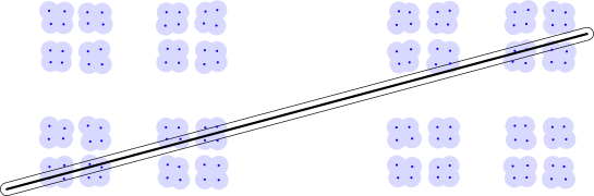
Figure 2. An illustration of Lemma 2.9 for $S=\mathbf{Y}$. The dots are the elements of the $r_{0}$-separated set $S$. The thick line is the segment $\tau$, which has length $r_{1}$. The oval shape is the neighborhood $\tau+B(0,2r_{0})$, and the blue shape is the neighborhood $\mathbf{Y}+B(0,3r_{0})$.

Proof.

1. Consider the set

$$\widetilde{Y}:=(\mathbf{Y}+B(0,3r_{0}))\cap\tau.$$

By Lemma 2.8, the set $\widetilde{Y}$ is $\nu\over 2$-porous on lines on scales $\widetilde{r}_{0}$ to $\rho_{1}$, where

$$\widetilde{r}_{0}:={6\over\nu}r_{0}.$$

Taking a unit speed parametrization of the line segment $\tau$, we can consider $\widetilde{Y}$ as a subset of $[0,r_{1}]\subset\mathbb{R}$. This set is $\nu\over 2$-porous on scales $\widetilde{r}_{0}$ to $\rho_{1}$. Thus by Lemma 2.7 with $I:=[0,r_{1}]$, we have, with $\delta$ given by (2.19) with $\nu$ replaced by $\nu\over 2$, and $|\bullet|$ denoting the one-dimensional Lebesgue measure on $\tau$,

$$|\widetilde{Y}|\leq r_{1}^{\delta}{\widetilde{r}_{0}}^{\,1-\delta}.$$ (2.21)

(Strictly speaking the above argument does not apply when $\widetilde{r}_{0}>\rho_{1}$, but in the latter case we have $\widetilde{r}_{0}>r_{1}$ and (2.21) is immediate since $|\widetilde{Y}|\leq|\tau|=r_{1}$.)

2. Denote $\widetilde{S}:=S\cap(\tau+B(0,2r_{0}))$. For each $\mathbf{x}\in\widetilde{S}$, the set

$$I_{\mathbf{x}}:=B(\mathbf{x},3r_{0})\cap\tau$$

is a line segment of length $\geq r_{0}$ inside $\tau$. Since $\widetilde{S}\subset S\subset\mathbf{Y}$, we have $I_{\mathbf{x}}\subset\widetilde{Y}$. Moreover, for any given $\mathbf{y}\in\tau$, if $\mathbf{y}\in I_{\mathbf{x}}$ then $\mathbf{x}\in B(\mathbf{y},3r_{0})$. Since $\widetilde{S}$ is an $r_{0}$-separated set, the ball $B(\mathbf{y},3r_{0})$ contains at most $100$ points in the set $\widetilde{S}$ (since the $r_{0}\over 2$-balls centered at these points are nonintersecting and contained in the ball $B(\mathbf{y},4r_{0})$). It follows that each point $\mathbf{y}\in\tau$ is contained in at most 100 intervals $I_{\mathbf{x}}$. We now estimate

$$r_{0}\#(\widetilde{S})\leq\sum_{\mathbf{x}\in\widetilde{S}}|I_{\mathbf{x}}|\leq 100\bigg{|}\bigcup_{\mathbf{x}\in\widetilde{S}}I_{\mathbf{x}}\bigg{|}\leq 100|\widetilde{Y}|.$$

Using (2.21), we get

$$\#(\widetilde{S})\leq{600\over\nu}\Big{(}{r_{1}\over r_{0}}\Big{)}^{\delta},$$

giving (2.20). ∎

3. Construction of a weight adapted to a line porous set

In this section we prove Theorem 3 following [Coh23, §6.1].

Let $\nu$ be the line porosity constant of the set $\mathbf{Y}$ and let $\delta\in(0,1)$ be the constant in Lemma 2.9. Fix constants $\eta,\alpha$ such that

$$0<\eta<\tfrac{1}{3},\quad 3\eta\leq\alpha<1,\quad\alpha>1-\eta(1-\delta).$$ (3.1)

To construct the weight $\omega_{k}$, take $k\geq 1$, put

$$r_{k}:={2^{k}\over k^{\eta}}$$

and let

$$S_{k}\ \subset\ \mathbf{Y}\cap\{2^{k-1}\leq|\mathbf{x}|\leq 2^{k+1}\}$$

be a maximal $r_{k}$-separated subset.

Fix cutoff functions

$$\begin{gathered}\chi,\psi\in C^{\infty}_{\mathrm{c}}(\mathbb{R}^{2};[0,1]),\quad\operatorname{supp}\chi\subset B(0,2),\quad\chi=1\text{ on }B(0,1);\\ \operatorname{supp}\psi\subset\{\tfrac{1}{2}<|\mathbf{x}|<2\},\quad\psi=1\text{ on }\{\tfrac{1}{\sqrt{2}}\leq|\mathbf{x}|\leq\sqrt{2}\}\end{gathered}$$

and put

$$\omega_{k}(\mathbf{x}):=-10\psi(2^{-k}\mathbf{x})\sum_{\mathbf{y}\in S_{k}}{2^{k}\over k^{\alpha}}\,\chi\Big{(}{\mathbf{x}-\mathbf{y}\over r_{k}}\Big{)}.$$ (3.2)

We show that $\omega_{k}$ satisfy all the conclusions of Theorem 3. Below $K$ denotes a global constant whose value may change from place to place.

• (1.9) holds since if $2^{k-1}>h^{-1}$, then $S_{k}=\emptyset$ and thus $\omega_{k}=0$.

• (1.10) follows immediately from the definition of $\omega_{k}$.

• To show the regularity property (1.11), we estimate for $|\gamma|\leq 3$ and all $\mathbf{x}\in\mathbb{R}^{2}$

  $$|\partial^{\gamma}_{\mathbf{x}}\omega_{k}(\mathbf{x})|\leq K{2^{k}\over k^{\alpha}}r_{k}^{-|\gamma|}\#(S_{k}\cap B(\mathbf{x},2r_{k}))\leq K2^{(1-|\gamma|)k}k^{|\gamma|\eta-\alpha}$$

  where in the last inequality we use that $S_{k}$ is an $r_{k}$-separated set and thus the ball $B(\mathbf{x},2r_{k})$ contains no more than 100 points in $S_{k}$. Since $|\gamma|\eta-\alpha\leq 3\eta-\alpha\leq 0$, we see that $\|\omega_{k}\|_{S^{1}_{3}}\leq K$, giving (1.11).

• To show the growth property (1.12), assume for now that $k$ satisfies $2^{k+2}\leq h^{-1}$. For $\theta\in\mathbb{S}^{1}$ consider the line segment

  $$\tau_{k,\theta}:=\{(t\cos\theta,t\sin\theta)\mid-2^{k+1}\leq t\leq 2^{k+1}\}\ \subset\ \mathbb{R}^{2}.$$

  For each $\mathbf{y}\in S_{k}$, if the support of $\chi\big{(}{\mathbf{x}-\mathbf{y}\over r_{k}}\big{)}$ intersects $\tau_{k,\theta}$, then $\mathbf{y}$ lies in the set

  $$\widetilde{S}_{k,\theta}:=S_{k}\cap(\tau_{k,\theta}+B(0,2r_{k})).$$

  By Lemma 2.9 with $\rho_{0}:=1$, $\rho_{1}:=h^{-1}$, $r_{0}:=r_{k}\geq 1$, $r_{1}:=2^{k+2}$, and the fact that $\mathbf{Y}$ is porous on lines, we have

  $$\#(\widetilde{S}_{k,\theta})\leq Ck^{\delta\eta}$$

  where the constant $C$ depends only on $\nu$. We now estimate (where $ds$ stands for arc length element)

  $$-T(|\mathbf{x}|^{-2}\omega_{k})(0,\theta) \leq-2^{2-2k}\int_{\tau_{k,\theta}}\omega_{k}(\mathbf{x})\,ds(\mathbf{x})$$

  $$\leq K\cdot 2^{-2k}\cdot\#(\widetilde{S}_{k,\theta})\cdot{2^{k}\over k^{\alpha}}\cdot r_{k}$$

  $$\leq KCk^{(\delta-1)\eta-\alpha}.$$

  This implies that, with $q_{k}:=-\inf_{\theta\in\mathbb{S}^{1}}T(|\mathbf{x}|^{-2}\omega_{k})(0,\theta)$, we have

  $$q_{k}\leq KCk^{(\delta-1)\eta-\alpha}\quad\text{when }2^{k+2}\leq h^{-1}.$$ (3.3)

  By the proof of (1.9) above, we know that $q_{k}=0$ when $2^{k-1}>h^{-1}$. Thus (3.3) is satisfied for all but 3 values of $k$. Since each $q_{k}$ is bounded by (1.14) and $(\delta-1)\eta-\alpha<-1$, we get

  $$\sum_{k=1}^{\infty}q_{k}\leq KC\sum_{k=1}^{\infty}k^{(\delta-1)\eta-\alpha}\leq KC,$$

  which gives (1.12).

• It remains to show the property (1.15). Take arbitrary $\mathbf{x}\in\mathbf{Y}\setminus B(0,10)$. Choose $k\geq 1$ such that

  $$2^{k-\frac{1}{2}}\leq|\mathbf{x}|\leq 2^{k+\frac{1}{2}}.$$ (3.4)

  Then $\psi(2^{-k}\mathbf{x})=1$. Since $S_{k}$ is a maximal $r_{k}$-separated subset of $\mathbf{Y}\cap\{2^{k-1}\leq|\mathbf{x}|\leq 2^{k+1}\}$, there exists $\mathbf{y}\in S_{k}$ such that $|\mathbf{x}-\mathbf{y}|\leq r_{k}$. We have $\chi\big{(}{\mathbf{x}-\mathbf{y}\over r_{k}}\big{)}=1$, thus from the definition (3.2) of $\omega_{k}$ we see that

  $$\omega(\mathbf{x})\leq\omega_{k}(\mathbf{x})\leq-10{2^{k}\over k^{\alpha}}\leq-{|\mathbf{x}|\over(\log|\mathbf{x}|)^{\alpha}}$$

  where in the last inequality we use (3.4). This finishes the proof of (1.15).

4. Plurisubharmonicity of the extended weight

This section (following [Coh23, §3]) gives a criterion for plurisubharmonicity of functions of the form (1.24) in terms of the X-ray transform. This is the first ingredient in the proof of Theorem 5.

Proposition 4.1.

Assume that $\omega\in C^{\infty}_{\mathrm{c}}(\mathbb{R}^{2};\mathbb{R})$ and $\sigma\in\mathbb{R}$. Define the function $u\in C^{0}(\mathbb{C}^{2};\mathbb{R})$ by

$$u(\mathbf{x}+i\mathbf{y})=E\omega(\mathbf{x}+i\mathbf{y})+\sigma|\mathbf{y}|,\quad\mathbf{x},\mathbf{y}\in\mathbb{R}^{2}.$$ (4.1)

Then $u$ is plurisubharmonic on $\mathbb{C}^{2}$ if and only if

$$T(\Delta\omega)(s,\theta)+\pi\sigma\geq 0\quad\text{for all }s\in\mathbb{R},\ \theta\in\mathbb{S}^{1}.$$ (4.2)

Remark 4.2.

In [Coh23, (3.5)] there is an extra condition needed for plurisubharmonicity, in terms of the derivative of the Hilbert transform of restrictions of $\omega$ to lines in $\mathbb{R}^{2}$. More precisely, one requires that for any $\mathbf{z}_{0},\mathbf{v}_{0}\in\mathbb{R}^{2}$ with $|\mathbf{v}_{0}|=1$, if we define $\omega_{0}(t):=\omega(\mathbf{z}_{0}+t\mathbf{v}_{0})$, then

$$\mathcal{H}\omega_{0}^{\prime}(0)\leq\sigma.$$ (4.3)

This condition corresponds to subharmonicity of the restriction of $u$ to the complex line $\{\mathbf{z}_{0}+w\mathbf{v}_{0}\mid w\in\mathbb{C}\}$. Our proof uses the distributional criterion for plurisubharmonicity, Proposition 2.6, and does not explicitly need the condition (4.3).

However, the extra condition (4.3) can be derived from (4.2) as follows. Since (4.2) is invariant under composition of $\omega$ with rotations and translations, we may assume that $\mathbf{z}_{0}=(0,0)$ and $\mathbf{v}_{0}=(1,0)$, that is $\omega_{0}(t)=\omega(t,0)$. By Lemma 2.3 we have

$$\mathcal{H}\omega_{0}^{\prime}(0)=-{1\over 4\pi}\int_{\mathbb{S}^{1}}|\sin\theta|\,T(\Delta\omega)(0,\theta)\,d\theta.$$

Assume that $\omega$ satisfies (4.2). Since $\int_{\mathbb{S}^{1}}|\sin\theta|\,d\theta=4$, we get the condition (4.3).

4.1. An auxiliary distribution

For each $t\in\mathbb{R}$, define the distribution

$$Z_{t}(x_{1}+iy_{1},x_{2}+iy_{2}):=\delta(x_{1}-ty_{1})\delta(x_{2}-ty_{2})\ \in\ \mathcal{D}^{\prime}(\mathbb{C}^{2}).$$

This family of distributions is integrable in $t$, more precisely we have the following

Lemma 4.3.

If $\varphi\in C^{\infty}_{\mathrm{c}}(\mathbb{C}^{2})$ and $\operatorname{supp}\varphi\subset B(0,R)$ for some $R\geq 0$, then

$$|(Z_{t},\varphi)|\leq\pi R^{2}\|\varphi\|_{C^{0}}\,\langle t\rangle^{-2}.$$ (4.4)

Proof.

We have

$$(Z_{t},\varphi)=\int_{\mathbb{R}^{2}}\varphi(ty_{1}+iy_{1},ty_{2}+iy_{2})\,dy_{1}dy_{2}.$$ (4.5)

The expression under the integral is supported in the ball $B(0,R/\langle t\rangle)$ and is bounded in absolute value by $\|\varphi\|_{C^{0}}$, which gives (4.4). ∎

We also have the following identity featuring the matrix $\partial_{\bar{\mathbf{z}}\mathbf{z}}Z_{t}$:

$$\partial_{\bar{\mathbf{z}}\mathbf{z}}Z_{t}={1+t^{2}\over 4}\,\partial_{\mathbf{x}}^{2}Z_{t},\qquad\partial_{\mathbf{x}}^{2}:=\begin{pmatrix}\partial_{x_{1}}^{2}&\partial_{x_{1}x_{2}}\\ \partial_{x_{1}x_{2}}&\partial_{x_{2}}^{2}\end{pmatrix}.$$ (4.6)

4.2. The extension operator as a convolution

We now write $E\omega$ as a distributional convolution. For $\psi\in C^{\infty}_{\mathrm{c}}(\mathbb{R}^{2})$, define the distribution

$$(\psi\otimes\delta)(x_{1}+iy_{1},x_{2}+iy_{2}):=\psi(x_{1},x_{2})\delta(y_{1})\delta(y_{2})\ \in\ \mathcal{E}^{\prime}(\mathbb{C}^{2}).$$

Then for each $t\in\mathbb{R}$ we have

$$(Z_{t}*(\psi\otimes\delta))(\mathbf{x}+i\mathbf{y})=\psi(\mathbf{x}-t\mathbf{y}).$$ (4.7)

By Lemma 4.3, the pairing of (4.7) with any test function $\varphi\in C^{\infty}_{\mathrm{c}}(\mathbb{C}^{2})$ is $\mathcal{O}(\langle t\rangle^{-2})$. In fact, we have the following bound on this distribution in $L^{1}_{\operatorname{loc}}(\mathbb{C}^{2})$:

Lemma 4.4.

Let $R>0$ and assume that $\operatorname{supp}\psi\subset B(0,R)$. Then we have

$$\|Z_{t}*(\psi\otimes\delta)\|_{L^{1}(B(0,R))}\leq 50R^{4}\|\psi\|_{C^{0}}\,\langle t\rangle^{-2}.$$ (4.8)

Proof.

By (4.7), the left-hand side of (4.8) is equal to

$$\int_{B(0,R)}|\psi(\mathbf{x}-t\mathbf{y})|\,d\mathbf{x}d\mathbf{y}.$$ (4.9)

If $(\mathbf{x},\mathbf{y})\in B(0,R)$ and $\psi(\mathbf{x}-t\mathbf{y})\neq 0$, then

$$|\mathbf{x}|,|\mathbf{y}|,|\mathbf{x}-t\mathbf{y}|\leq R,$$

which in turn implies that $|t\mathbf{y}|\leq 2R$ and thus $|\mathbf{y}|\leq\sqrt{5}R\langle t\rangle^{-1}$. Thus we can bound the integral in (4.9) by the integral over $\{|\mathbf{x}|\leq R,\ |\mathbf{y}|\leq\sqrt{5}R\langle t\rangle^{-1}\}$, which is a set of volume $5\pi^{2}R^{4}\langle t\rangle^{-2}\leq 50R^{4}\langle t\rangle^{-2}$. This gives (4.8). ∎

By Lemma 4.4, the function $Z_{t}*(\psi\otimes\delta)$ is integrable in $t$ with values in $L^{1}_{\operatorname{loc}}(\mathbb{C}^{2})$, which by Fubini’s Theorem is equivalent to $Z_{t}*(\psi\otimes\delta)$ being integrable on $\mathbb{R}_{t}\times B(0,R)_{(\mathbf{x},\mathbf{y})}$ for each $R$. The next lemma computes the integral of $Z_{t}*(\psi\otimes\delta)$ in $t$ in terms of the X-ray transform of $\psi$:

Lemma 4.5.

For any $\psi\in C^{\infty}_{\mathrm{c}}(\mathbb{R}^{2})$, we have

$$\int_{\mathbb{R}}(Z_{t}*(\psi\otimes\delta))(\mathbf{x}+i\mathbf{y})\,dt={1\over r}\,T\psi(x_{2}\cos\theta-x_{1}\sin\theta,\theta)$$ (4.10)

where we write $\mathbf{x}=(x_{1},x_{2})$, $\mathbf{y}=(r\cos\theta,r\sin\theta)$ with $r>0$, $\theta\in\mathbb{S}^{1}$, and the integral is understood in $L^{1}_{\operatorname{loc}}(\mathbb{C}^{2})$.

Proof.

It suffices to check that the formula (4.10) holds pointwise for each $\mathbf{x}\in\mathbb{R}^{2}$, $\mathbf{y}\in\mathbb{R}^{2}\setminus\{0\}$. Using (4.7) we compute

$$\begin{gathered}\int_{\mathbb{R}}(Z_{t}*(\psi\otimes\delta))(\mathbf{x}+i\mathbf{y})\,dt=\int_{\mathbb{R}}\psi(x_{1}-rt\cos\theta,x_{2}-rt\sin\theta)\,dt\\ ={1\over r}\int_{\mathbb{R}}\psi(\tilde{t}\cos\theta-(x_{2}\cos\theta-x_{1}\sin\theta)\sin\theta,\tilde{t}\sin\theta+(x_{2}\cos\theta-x_{1}\sin\theta)\cos\theta)\,d\tilde{t}\\ ={1\over r}\,T\psi(x_{2}\cos\theta-x_{1}\sin\theta,\theta)\end{gathered}$$

giving (4.10). Here in the second line we make the change of variables $\tilde{t}=-rt+x_{1}\cos\theta+x_{2}\sin\theta$. ∎

Using the above lemmas, we now compute the matrix of distributional derivatives $\partial_{\bar{\mathbf{z}}\mathbf{z}}E\omega$:

Lemma 4.6.

Let $\omega\in C^{\infty}_{\mathrm{c}}(\mathbb{R}^{2})$. Then the entries of the matrix $\partial_{\bar{\mathbf{z}}\mathbf{z}}E\omega$ lie in $L^{1}_{\operatorname{loc}}(\mathbb{C}^{2})$ and we have

$$\partial_{\bar{\mathbf{z}}\mathbf{z}}E\omega(\mathbf{x}+i\mathbf{y})={1\over 4\pi r}\,T(\partial_{\mathbf{x}}^{2}\omega)(x_{2}\cos\theta-x_{1}\sin\theta,\theta)$$ (4.11)

where we write $\mathbf{x}=(x_{1},x_{2})$, $\mathbf{y}=(r\cos\theta,r\sin\theta)$ with $r>0$, $\theta\in\mathbb{S}^{1}$.

Proof.

Comparing (1.22) with (4.7), we express $E\omega$ as a distributional convolution: for each $\omega\in C^{\infty}_{\mathrm{c}}(\mathbb{R}^{2})$

$$E\omega={1\over\pi}\int_{\mathbb{R}}{Z_{t}*(\omega\otimes\delta)\over 1+t^{2}}\,dt.$$

Using (4.6) and the properties of convolution under differentiation we compute

$$\partial_{\bar{\mathbf{z}}\mathbf{z}}E\omega ={1\over\pi}\int_{\mathbb{R}}{(\partial_{\bar{\mathbf{z}}\mathbf{z}}Z_{t})*(\omega\otimes\delta)\over 1+t^{2}}\,dt$$

$$={1\over 4\pi}\int_{\mathbb{R}}(\partial_{\mathbf{x}}^{2}Z_{t})*(\omega\otimes\delta)\,dt$$

$$={1\over 4\pi}\int_{\mathbb{R}}{Z_{t}*(\partial_{\mathbf{x}}^{2}\omega\otimes\delta)}\,dt.$$

Here by Lemma 4.4 the integrals above converge in $L^{1}_{\operatorname{loc}}(\mathbb{C}^{2})$. It remains to use Lemma 4.5 for the functions $\psi:=\partial_{x_{j}}\partial_{x_{k}}\omega$. ∎

4.3. End of the proof

We are now ready to give

Proof of Proposition 4.1.

1. We first compute

$$\partial_{\bar{\mathbf{z}}\mathbf{z}}|\mathbf{y}|={1\over 4r}A_{\theta},\quad A_{\theta}:=\begin{pmatrix}\sin^{2}\theta&-\sin\theta\cos\theta\\ -\sin\theta\cos\theta&\cos^{2}\theta\end{pmatrix}.$$ (4.12)

Here we write $\mathbf{y}=(r\cos\theta,r\sin\theta)$ with $r>0$ and $\theta\in\mathbb{S}^{1}$, differentiation is understood in the sense of distributions on $\mathbb{C}^{2}$, and (4.12) has entries in $L^{1}_{\operatorname{loc}}(\mathbb{C}^{2})$. To see (4.12) we first note that both sides only depend on $\mathbf{y}=\operatorname{Im}\mathbf{z}$ and thus can be considered as distributions on $\mathbb{R}^{2}$. Now (4.12) can be verified by direct computation on $\mathbb{R}^{2}\setminus\{0\}$, where the function $|\mathbf{y}|$ is smooth, and extends to an identity in the sense of distributions on the entire $\mathbb{R}^{2}$ by homogeneity, see for example [Hör03, Theorem 3.2.3].

2. Recall that $u=E\omega+\sigma|\mathbf{y}|$. Combining Lemma 4.6 and (4.12) we see that

$$4\pi\partial_{\bar{\mathbf{z}}\mathbf{z}}u(\mathbf{x}+i\mathbf{y})={1\over r}\big{(}T(\partial_{\mathbf{x}}^{2}\omega)(x_{2}\cos\theta-x_{1}\sin\theta,\theta)+\pi\sigma A_{\theta}\big{)}.$$ (4.13)

Here derivatives are understood in the sense of distributions on $\mathbb{C}^{2}$ and (4.13) has entries in $L^{1}_{\operatorname{loc}}(\mathbb{C}^{2})$.

By Proposition 2.6, we see that $u$ is plurisubharmonic if and only if

$$\big{\langle}\big{(}T(\partial_{\mathbf{x}}^{2}\omega)(s,\theta)+\pi\sigma A_{\theta}\big{)}\mathbf{v},\mathbf{v}\big{\rangle}_{\mathbb{C}^{2}}\geq 0\quad\text{for all }s\in\mathbb{R},\ \theta\in\mathbb{S}^{1},\ \mathbf{v}\in\mathbb{C}^{2}.$$ (4.14)

Since $\omega$ is real-valued, the matrix on the left-hand side has real entries. Therefore, it suffices to verify (4.14) for all vectors of the form $\mathbf{v}_{\gamma}=(\cos\gamma,\sin\gamma)$ where $\gamma\in\mathbb{S}^{1}$. Using Lemma 2.1 we compute

$$\big{\langle}\big{(}T(\partial_{\mathbf{x}}^{2}\omega)(s,\theta)+\pi\sigma A_{\theta}\big{)}\mathbf{v}_{\gamma},\mathbf{v}_{\gamma}\big{\rangle}_{\mathbb{C}^{2}} =T(V_{\gamma}^{2}\omega)(s,\theta)+\pi\sigma\sin^{2}(\theta-\gamma)$$

$$=\big{(}T(\Delta\omega)(s,\theta)+\pi\sigma\big{)}\sin^{2}(\theta-\gamma).$$

It follows that (4.14) is equivalent to

$$T(\Delta\omega)(s,\theta)+\pi\sigma\geq 0\quad\text{for all }s\in\mathbb{R},\ \theta\in\mathbb{S}^{1}$$

which finishes the proof. ∎

5. Proof of Theorem 5

In this section we finish the proof of Theorem 5 by constructing a weight $\widetilde{\omega}\leq\omega$ which satisfies the X-ray transform condition (4.2). We follow [Coh23, §4].

5.1. Weights with constant radial integrals

We start with the special case when for each $k$, the integral of $|\mathbf{x}|^{-2}\omega_{k}$ on lines through the origin is constant (i.e. does not depend on the choice of the line). In this case the $\partial_{\theta}^{2}$ term in Lemma 2.2 disappears and we can take $\widetilde{\omega}:=\omega$ in Theorem 5.

Proposition 5.1.

Assume that $\omega$ is given by (1.8) where $\omega_{k}$ satisfy the conditions (1.9)–(1.12) for some constants $C_{\mathrm{reg}},C_{\mathrm{gr}}$. Assume moreover that for all $k\geq 1$ and $\theta\in\mathbb{S}^{1}$

$$T(|\mathbf{x}|^{-2}\omega_{k})(0,\theta)=-q_{k}$$ (5.1)

where $q_{k}$ depends on $k$ but does not depend on $\theta$. Then for $\sigma\geq 0$ large enough depending only on $C_{\mathrm{reg}},C_{\mathrm{gr}}$ the function $u$ defined by (4.1) is plurisubharmonic on $\mathbb{C}^{2}$.

Proof.

Throughout the proof the letter $K$ denotes a global constant whose value may change from place to place.

1. By Proposition 4.1, it suffices to show that for $\sigma$ large enough depending only on $C_{\mathrm{reg}},C_{\mathrm{gr}}$ we have

$$T(\Delta\omega)(s,\theta)+\pi\sigma\geq 0\quad\text{for all }s\in\mathbb{R},\ \theta\in\mathbb{S}^{1}.$$ (5.2)

We first consider the special case $s=0$. In this case by Lemma 2.2 and (5.1) we compute

$$T(\Delta\omega_{k})(0,\theta)=-q_{k}\quad\text{for all }k\geq 1,\ \theta\in\mathbb{S}^{1}.$$ (5.3)

Together with (1.12) this shows that (5.2) holds for $s=0$ as long as $\pi\sigma\geq C_{\mathrm{gr}}$.

To handle the case of general $s$, we will show the following estimate which only needs the conditions (1.9)–(1.11):

$$\bigg{|}T(\Delta\omega)(s,\theta)-\sum_{k\geq 1\atop 2^{k+1}\geq|s|}T(\Delta\omega_{k})(0,\theta)\bigg{|}\leq KC_{\mathrm{reg}}.$$ (5.4)

Together with (5.3), (1.12), and the fact that $q_{k}\geq 0$ this shows that (5.2) holds as long as $\pi\sigma\geq C_{\mathrm{gr}}+KC_{\mathrm{reg}}$.

2. It remains to show (5.4). By the discrete symmetry (2.1) and equivariance under rotations (2.3) we reduce to the case when $\theta=0$ and $s\geq 0$, that is it suffices to show that

$$\bigg{|}T(\Delta\omega)(s,0)-\sum_{k\geq 1\atop 2^{k+1}\geq s}T(\Delta\omega_{k})(0,0)\bigg{|}\leq KC_{\mathrm{reg}}.$$ (5.5)

Fix $s\geq 0$. If $k$ is such that $2^{k+1}<s$, then by (1.10) the support of $\Delta\omega_{k}$ lies in the ball $B(0,s)$ and thus $T(\Delta\omega_{k})(s,0)=0$. Thus (5.5) becomes

$$\bigg{|}\sum_{k\geq 1\atop 2^{k+1}\geq s}\int_{\mathbb{R}}\big{(}\Delta\omega_{k}(x_{1},s)-\Delta\omega_{k}(x_{1},0)\big{)}\,dx_{1}\bigg{|}\leq KC_{\mathrm{reg}}.$$ (5.6)

By the triangle inequality and the fundamental theorem of calculus in the $x_{2}$ variable, the left-hand side of (5.6) is bounded by

$$\sum_{k\geq 1\atop 2^{k+1}\geq s}\int_{\mathbb{R}\times[0,s]}\big{|}\partial_{x_{2}}\Delta\omega_{k}(x_{1},x_{2})\big{|}\,dx_{1}dx_{2}.$$

By (1.11) and (1.10) we have $\sup|\partial_{x_{2}}\Delta\omega_{k}|\leq KC_{\mathrm{reg}}2^{-{2k}}$. On the other hand, by (1.10) the intersection of $\mathbb{R}\times[0,s]$ with $\operatorname{supp}\partial_{x_{2}}\Delta\omega_{k}$ is contained in $[-2^{k+1},2^{k+1}]\times[0,s]$, which has area $2^{k+2}s$. It follows that the left-hand side of (5.6) is bounded by

$$KC_{\mathrm{reg}}\,s\sum_{k\geq 1\atop 2^{k+1}\geq s}2^{-k}\leq KC_{\mathrm{reg}},$$

finishing the proof of (5.4). ∎

5.2. Modifying a general weight

We now give

Proof of Theorem 5.

1. Assume that $\omega$ is given by (1.8) where $\omega_{k}$ satisfy the conditions (1.9)–(1.12) for some constants $C_{\mathrm{reg}},C_{\mathrm{gr}}$. We subtract a function from each $\omega_{k}$ to obtain a weight $\widetilde{\omega}_{k}$ satisfying the additional condition (5.1). To do this, fix a cutoff function

$$\chi\in C^{\infty}_{\mathrm{c}}\big{(}(-2,-\tfrac{1}{2})\cup(\tfrac{1}{2},2);[0,\infty)\big{)},\quad\chi(-t)=\chi(t),\quad\int_{\mathbb{R}}t^{-2}\chi(t)\,dt=1.$$

For each $k\geq 1$, define the function $\psi_{k}\in C^{\infty}_{\mathrm{c}}(\mathbb{R}^{2}\setminus\{0\})$ in polar coordinates: for $t\in\mathbb{R}$ and $\theta\in\mathbb{S}^{1}$ put

$$\psi_{k}(t\cos\theta,t\sin\theta):=2^{k}\chi(2^{-k}t)\big{(}T(|\mathbf{x}|^{-2}\omega_{k})(0,\theta)+q_{k}\big{)}.$$

Now, define the modified weight

$$\widetilde{\omega}:=\sum_{k\geq 1}\widetilde{\omega}_{k}\quad\text{where }\widetilde{\omega}_{k}:=\omega_{k}-\psi_{k}.$$

2. We show several properties of $\widetilde{\omega}_{k}$. Recall from (1.12) that

$$q_{k}:=-\inf_{\theta\in\mathbb{S}^{1}}T(|\mathbf{x}|^{-2}\omega_{k})(0,\theta).$$

It follows that $\psi_{k}\geq 0$ and thus $\widetilde{\omega}_{k}\leq\omega_{k}$. This shows that $\widetilde{\omega}\leq\omega$.

It is easy to see that $\widetilde{\omega}_{k}$ satisfy the conditions (1.9)–(1.10). Moreover, by (2.16) and (2.17) we see that $\|\widetilde{\omega}_{k}\|_{S^{1}_{3}}\leq K\|\omega_{k}\|_{S^{1}_{3}}$ for some global constant $K$. Therefore $\widetilde{\omega}_{k}$ satisfy the Kohn–Nirenberg regularity condition (1.11) with constant $KC_{\mathrm{reg}}$ where $C_{\mathrm{reg}}$ is the constant in the regularity condition (1.11) for $\omega_{k}$.

Finally, we compute for each $\theta\in\mathbb{S}^{1}$

$$T(|\mathbf{x}|^{-2}\widetilde{\omega}_{k})(0,\theta)=T(|\mathbf{x}|^{-2}\omega_{k})(0,\theta)-\int_{\mathbb{R}}t^{-2}\,\psi_{k}(t\cos\theta,t\sin\theta)\,dt=-q_{k}.$$

Therefore, $\widetilde{\omega}_{k}$ satisfy the additional condition (5.1) and thus also the growth condition (1.12) (with the same values of $q_{k}$ as for $\omega_{k}$).

3. It remains to apply Proposition 5.1 with $\omega_{k}$ replaced by $\widetilde{\omega}_{k}$ to see that for $\sigma$ large enough depending only on $C_{\mathrm{reg}},C_{\mathrm{gr}}$, the function $\widetilde{u}$ defined by (1.24) is plurisubharmonic on $\mathbb{C}^{2}$. ∎

Acknowledgements. I am grateful to Alex Cohen for sharing the early versions of [Coh23] with me and many discussions. I was supported by NSF CAREER grant DMS-1749858.

References

- [BD18] Jean Bourgain and Semyon Dyatlov. Spectral gaps without the pressure condition. Ann. of Math. (2), 187(3):825–867, 2018.
- [Coh23] Alex Cohen. Fractal uncertainty in higher dimensions, 2023. arXiv:2305.05022v1.
- [Dya19] Semyon Dyatlov. An introduction to fractal uncertainty principle. J. Math. Phys., 60(8):081505, 31, 2019.
- [Hör03] Lars Hörmander. The analysis of linear partial differential operators. I. Classics in Mathematics. Springer-Verlag, Berlin, 2003. Distribution theory and Fourier analysis, Reprint of the second (1990) edition [Springer, Berlin; MR1065993 (91m:35001a)].
- [HS20] Rui Han and Wilhelm Schlag. A higher-dimensional Bourgain-Dyatlov fractal uncertainty principle. Anal. PDE, 13(3):813–863, 2020.