Unsupervised machine learning for identifying phase transition using two-times clustering

Abstract

In recent years, developing unsupervised machine learning for identifying phase transition is a research direction. In this paper, we introduce a two-times clustering method that can help select perfect configurations from a set of degenerate samples and assign the configuration with labels in a manner of unsupervised machine learning. These perfect configurations can then be used to train a neural network to classify phases. The derivatives of the predicted classification in the phase diagram, show peaks at the phase transition points. The effectiveness of our method is tested for the Ising, Potts, and Blume-Capel models. By using the ordered configuration from two-times clustering, our method can provide a useful way to obtain phase diagrams.

Figure 1: The main idea of the two-times clustering method. (a) In the plane $(D,h)$, the parameter intervals are gridded in preparation for sampling. (b) For each parameter point, 100 configurations are sampled. (c) The first-time clustering determines the cluster centers for 100 samples at each parameter point. (d) The configurations with the same cluster center are given the same labels. (e) The second-time clustering determines the cluster centers of all samples in the whole parameter space. (f) and (g) The clusters are compared in pairs and similarity is judged based on the indexes of the clusters. (h) Groups with high similarity are considered to be in the same phase and given the same labels.

I Introduction

Since the pioneering work of J. Carrasquilla and R. G. Melko on applying machine learning (ML) methods to study spin systems [1], predicting the phase diagrams of interacting spin systems using ML has become an area of research interest [2]. Unsupervised ML methods are particularly useful in predicting phase diagrams as they do not require prior knowledge of the data labels. Common unsupervised ML methods include principal component analysis [3, 4, 5], t-distributed stochastic neighbor embedding [6, 7], diffusion maps [8, 9, 10, 11], the confusion method [12], the active contour model (snake model) [13, 14], Calinski-Harabaz index[15, 16], and many others. Various indicators always signal at the phase transition point.

Sometimes, unsupervised methods incorporate certain steps of supervised learning. For example, the confusion method [12] determines labels to train the neural network (NN) based on guessed phase transition points. The best-guessed transition point is then determined based on the performance (accuracy) of the NN. In the NN-based snake model [13, 14], the learning network in the NN also needs to be trained by data and dynamical labels while cooperating with the other guessing network.

In contrast, Refs. [17] applied theoretical ground state configurations in the ordered phase as the training set to train the neural network without using real data, and the method was found to be effective for the Potts model. D.-R. Tan and F.-J. Jiang [18] even used datasets with only 0’s and 1’s to train the network and predict the critical points of the XY model and the $O(3)$ model. Indeed, the identification of ordered phases is crucial for predicting phase transitions accurately.

In this paper, we propose a two-times clustering method to identify ordered configurations and their corresponding labels from numerical simulations. In the first clustering step, we select representative configurations from each physical parameter point. In the second clustering step, we obtain perfect configurations and their corresponding labels. These selected perfected configurations and labels are then used to train the neural network, and the neural network is tested with real simulated data and mapped to a phase diagram.

The reason for performing the second clustering step is to prevent the neural network from misidentifying degenerate states as belonging to different phases. For example, this step of clustering avoids treating the ordered state configurations of the four lattice sites Ising model $\uparrow\uparrow\uparrow\uparrow$, $\downarrow\downarrow\downarrow\downarrow$ as two different phases. The first step of classification involves selecting the perfect configurations from the data obtained through a real Monte Carlo (MC) simulation.

Our approach is essentially unsupervised despite utilizing neural networks for training and testing, as we do not know beforehand how many phases are included in the phase diagram. The $K$-means clustering algorithm [19] is employed for clustering, which provides us with a group center or configuration. The number of perfect configurations is selected based on the criterion that the center of the cluster corresponds to the lowest energy configuration. In the second clustering step, the perfect configurations obtained from the first clustering step under all phase diagram parameter points are merged and clustered again.

We mainly choose the BC model [20] to test our method. The BC model on the square lattice is defined by the following Hamiltonian:

$$H=-J_{x}\sum_{<i,j>_{x}}S_{i}S_{j}-J_{y}\sum_{<i,j>_{y}}S_{i}S_{j}+D\sum_{i}S_{i}^{2}-h\sum_{i}S_{i}$$ (1)

where $S_{i}=\pm 1,0,i=1,2\cdots N$, $N$ represents the total number of sites and $J_{x(y)}$ is the exchange interaction between sites along the two directions. $D$ is a single-spin anisotropy parameter and $h$ is an external magnetic field. The stripe-like pattern corresponds to the states $\begin{smallmatrix}+-\\ +-\end{smallmatrix}$, or $\begin{smallmatrix}+0\\ +0\end{smallmatrix}$. The uniform pattern corresponds to the states $\begin{smallmatrix}++\\ ++\end{smallmatrix}$, and $\begin{smallmatrix}00\\ 00\end{smallmatrix}$, respectively. The symbols “+”, “-”, and “0” correspond to the values taken by the spins. The phase diagram has been tested by the snake-net model [14].

By testing, we obtain two-dimensional planar phase diagrams of the BC model in an unsupervised manner, and even three-dimensional phase diagrams can be obtained. In order to understand the method, we have also illustrated the two-dimensional Ising model and Potts model [21] as examples.

The outline of this paper is as follows. In Sec. II, we present the methods including the two-times clustering, total procedure, and network structure. The first time clustering obtains the perfect configuration at the cluster center with each parameter point and the second time clustering obtains configurations and labels at the cluster centers with all parameter points. And then the similarity test is performed to merge the similar configuration and assign them the same labels.

In Sec. III, the method is applied to the two-dimensional Ising, Potts, and BC models. For the Ising and Potts models, instead of using two-time clustering, we directly use the 2*2 perfect configuration as the kernel matrix and thus calculate the similarity. For the BC model, the perfect configuration and labels are used from the two-times clustering. With them, the similarity degree is obtained by the neural networks. Both the 2D and 3D phase diagrams are obtained. The conclusion and discussion are presented in Sec. IV.

II Methods

II.1 Two-times of clustering

II.1.1 The first clustering

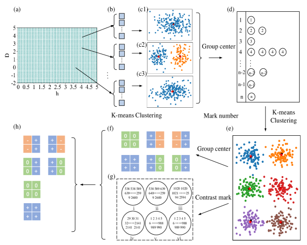
In Figs. 1 (a)-(b), a two-dimensional parameter space is constructed with $D$-$h$ variables, where $D$ is chosen to belong to the range [-2,5] and $h$ to belong to [0,5]. The two dimensions are discretized by 51 points each, resulting in a total of $51\times 51$ parameter points. Monte Carlo simulations are then conducted for each parameter point ($D_{i}$, $h_{i}$), generating 100 spin configurations with a size of 16 $\times$ 16.

In Fig. 1 (c), K-means clustering is performed on the 100 spin configurations generated at each parameter point. K-means clustering is an iterative unsupervised learning algorithm used for partitioning data into $n_{c}$ clusters. Given an input dataset ${\boldsymbol{D}}$ and the number of clusters, the algorithm outputs the classification centers and the corresponding cluster labels for each sample. The resulting clusters are typically presented in two-dimensional or high-dimensional plots, and the challenge is to determine the optimal number of clusters.

Here, some physical factors need to be considered. We try the number of clusters in turn, say $n_{c}=1,2,3,4,\cdots$, and then compare the average energy $E_{i},i\in[1,n_{c}]$ corresponding to the samples at the center of the clusters. The number of categories $n_{c}^{min}$ with the lowest energy is selected. Usually the clustering center ${\mathbf{X}}_{c}$ given by Kmeans is not a real sample, marked by the red points in the scatter plot in Figs. 1 (c). We choose the true sample ${\mathbf{X}^{\prime}}_{c}$ with the closest Euclidean distance to be the cluster center.

The purpose of selecting the cluster centers is to pick out ordered ground states, such as $\begin{smallmatrix}++\\ ++\end{smallmatrix}$, and $\begin{smallmatrix}00\\ 00\end{smallmatrix}$, respectively. In Figs. 1 (c1) and (c2), only one sample (represented by a red dot) and two samples (represented by red dots) are selected and passed on to the data sets in Fig. 1 (d). In actual simulations or real experimental data, the data has thermodynamic or quantum fluctuations. Or some possible meta-stable states where the system does not reach thermal equilibrium due to algorithmic limitations.

II.1.2 The second clustering

In the second-time clustering, we Perform clustering on the samples in Fig. 1 (d), and six clusters are obtained in Fig. 1 (e) via K-means lustering and Calinski-Harabaz index[15], which has been used for detecting topological phases[16]. The configuration at the center of each cluster is shown in Fig. 1 (f), and each configuration can be identified by its corresponding identity number.

Figure 2: Overlap degree versus classification

Figure 3: The structure of the neural network. The input data size is 16*16. C: convolution layer, generating 16 feature maps of 15*15. S: pooling layer, generating 16 feature maps of 5*5. N1: The first fully connected layer with 16 neurons. N2: The output layer with 4 neurons. The output similarity degree $P$ is the average probability of the four categories.

In Fig. 1 (g), there are six clusters represented by circles, with each circle containing numerous ID numbers of the samples within the cluster. To measure the similarity between two clusters, we perform a similarity test separately for the ID numbers in each circle. The similarity measure used here is a commonly employed method in machine learning and statistics.

We first select a cluster $G_{i}$, and then search for all ID numbers in any of the groups $G_{j}=1,\cdots,6$. We count the number of overlapping ID numbers found and define the overlap degree $O_{d}(i,j)$ as the number of overlapping ID numbers between $G_{i}$ and $G_{j}$ divided by the total number of ID numbers in $G_{i}$. For example, if $G_{i}={1,2,3}$ and $G_{j}={2,3,4,5}$, then $O_{d}(i,j)=2/3$.

In Fig. 2, we observe the overlap degree between different categories calculated using the similarity measure as described earlier. For example, the overlap degree for a category with itself, $O_{d}(a,a)$, is marked by green color and has a value of 1. Additionally, we can see several small values for $O_{d}(a,j),j\neq a$, which represents the degree of overlap between the different categories. Furthermore, categories $c$ and $d$ exhibit a high overlap degree of over 85$\%$, indicating that they are essentially the same category and should be grouped together.

II.2 Total steps

To obtain the phase diagram, we follow a three-step process:

(a) Input data engineering. Firstly, we use the Monte Carlo algorithm to generate spin configurations for the BC model on a two-dimensional 16 $\times$ 16 square lattice. These configurations are then assigned labels using the two-step clustering method illustrated in Fig. 1. The resulting labeled configurations $C_{i}$ are used in the subsequent steps.

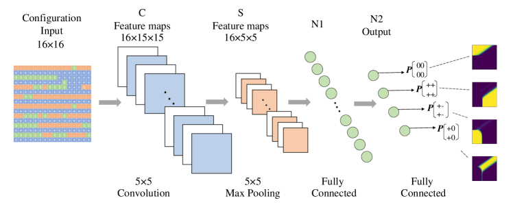
(b) Training and testing the neural network. As shown in Fig. 3, we use a convolutional neural network to classify the input configurations. The network is trained using the perfect configurations and labels from two-times clustering, and the entire data set is then input to the network for classification. The resulting classifications $P_{i}$ are recorded for each configuration.

(c) Mapping out the phase diagram. For each point $(x,y)$ in the parameter space, we calculate the gradients of the similarities $P_{i}$ with respect to $x$ and $y$ using the formulas:

$$E_{i}(x,y) =-|\nabla_{x}P_{i}|^{2}-|\nabla_{y}P_{i}|^{2},$$ (2)

$$E(x,y) =\sum_{i=1}^{N_{p}}E_{i}(x,y),$$ (3)

where $N_{p}$ is the number of possible phases. The sum of the negative gradients provides information at each point in the parameter space. At the phase transition boundary, the change in similarity $P$ is the most significant, and consequently, the gradient is the largest. To extract the phase boundaries, we utilize a method inspired by the active contours model called the snake model [22, 13, 14].

The snake model employs energy minimization to identify contour or boundary lines in an image. Using this model, we define the energy of the image in Eq. 3. This energy function enables us to trace and extract the phase boundaries in the parameter space.

III Results

III.1 2D Ising and Potts models

Figure 4: (a) Schematic diagram of the XNOR operation. Comparing the input configuration and the kernel matrix element, the same is assigned a value of 1, while the difference gets a value of 0 and then local similarity $p_{i,j}$ is obtained. (b) A possible configuration of the 4-state Potts model and their kernels. The results $P(T)$ and $-|\frac{\partial P(T)}{\partial T}|^{2}$ from (c) the Ising model and (d) the Potts model. The red dashed line marks the location of the predicted phase transition point.

The phase transition points of the 2D Ising model and the Potts model [21] are used as examples to explain the meaning of similarity $P_{i}(x,y)$ and its image energy $E(x,y)$. Because only the temperature parameter is varied, the phase diagram is one-dimensional. At low temperatures, the ground state of the ferromagnetic system is very readily available. Instead of choosing the perfect configurations by clustering twice, they are given here directly.

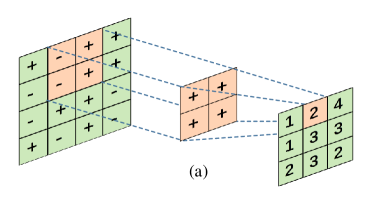
As shown in Fig. 4 (a), $P_{i}$ is obtained in a similar to 2D convolution. For the Ising model, one first defines a kernel matrix as

$$w^{+}=\begin{pmatrix}1&1\\ 1&1\end{pmatrix},\hskip 8.5359ptw^{-}=\begin{pmatrix}-1&-1\\ -1&-1\end{pmatrix}$$ (4)

and the kernel matrix element is all 1, representing a ground state a perfect configuration of the two-dimensional ferromagnetic Ising model. It is also feasible to use another perfect configuration that is all -1. Here, we use two kernel matrices in Eq. 4.

The XNOR operation calculates the similarity degree of the kernel and the lattice by sliding the kernel through the entire lattice. The similarity for the Ising model is defined as follows:

$$p_{i,j}^{+,-}=\sum_{m=1}^{kx}\sum_{n=1}^{ky}XNOR(w_{m,n}^{+,-},S_{i+m-1,j+n-1}).$$ (5)

In this equation, $S_{i+m-1,j+n-1}$ represents the spin of the $(i+m-1)$-th row and $(j+n-1)$-th column of the input configuration. Additionally, $kx$ and $ky$ represent the width and height of the convolutional-like XNOR kernel, respectively. The function $XNOR(A,B)$ returns 1 if $A==B$ and 0 if $A\neq B$. The variable $p_{i,j}$ represents the local similarity degree of the $(i,j)$-th element of the lattice after the operation.

To calculate the total similarity, we first compare the local similarity $p_{i,j}^{+}$ and $p_{i,j}^{-}$ obtained from different kernels, take their maximum values and finally sum up to get the total similarity $P$, defined as

$$P_{Ising} =\sum_{i,j}max(p_{i,j}^{+},p_{i,j}^{-}),$$ (6)

$$P_{q=4,Potts} =\sum_{i,j}max(p_{i,j}^{1},p_{i,j}^{2},p_{i,j}^{3},p_{i,j}^{4}).$$ (7)

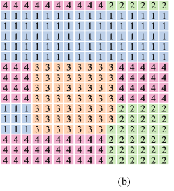
At temperature $T<T_{c}$, the 4-state Potts model is likely to have the configuration shown in Fig. 4 (b). In the lattice, there are several blocks, and the spins are the same within each block. There are domain walls between the blocks, caused by thermal excitation. This configuration is not the most perfectly ordered phase, e.g., all $1$, but it can still be ordered. For this purpose, we compare the similarity of $p_{i,j}^{i}$, $i=1,\cdots,4$, and take the maximum value as defined in Eq. 7 rather than take the average, which can not reflect the property of the phase very well.

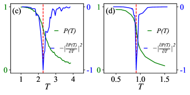
The results are shown in Fig. 4 (c) and (d). For the Ising and Potts models, the similarity degree $P$ measures the similarity between the spin configurations. $P(T)$ is marked by two green lines, and $P(T)$ is high at low temperatures ordered phase and decreases at high temperatures disordered phase.

To get the critical points, one has to measure the image energy defined by

$$E(T)=-\sum_{i}|\frac{\partial P_{i}(T)}{\partial T}|^{2}.$$ (8)

Actually, for the Ising model, $T_{c}^{Ising}$ can be determined analytically as:

$$T_{c}^{Ising}/J=2/\ln(1+\sqrt{2})\approx 2.269,$$ (9)

where $J$ is the coupling constant between neighboring spins. The critical behavior is reflected in the gradient of $P(T)$ with respect to temperature $T$, which exhibits a peak at $T_{c}^{Ising}$. The critical temperature of the Potts model can be computed by:

$$T_{c}^{Potts}/J=1/{\ln(1+\sqrt{4})}=0.9102.$$ (10)

Similar to the Ising model, the critical temperature is marked by a peak in the gradient of $P(T)$. The positions of the peak are located at 2.27 and 0.915, equal to the exact values within the intervals 0.01 respectively. In summary, the similarity degree $P(T)$ and its derivatives enable us to identify the phase transition points.

III.2 The Blume-Capel Model

Figure 5: (a) Two-dimensional BC model, the image energy $E$ from the gradient of similarity degree $P$ in the plane ($D-h)$. (b) Real data corresponds to the results in Fig. 1 (e). Six colors represent six clusters, pending a similarity test. The corresponding relation between each cluster and configuration are: a $\begin{smallmatrix}++\\ ++\end{smallmatrix}$, b $\begin{smallmatrix}--\\ --\end{smallmatrix}$, c $\begin{smallmatrix}-+\\ -+\end{smallmatrix}$, d $\begin{smallmatrix}0+\\ 0+\end{smallmatrix}$, e $\begin{smallmatrix}+-\\ +-\end{smallmatrix}$ and f $\begin{smallmatrix}+0\\ +0\end{smallmatrix}$.

III.2.1 Two-dimensional phase diagram of the BC model

The phase diagram of the BC model is known to be very rich [20]. It has been shown to be a convenient model for testing machine learning algorithms [14]. We use the proposed method illustrated in Fig. 1. Firstly, we generate input data in the parameter space $D-h$ using the Monte Carlo method. Then, we carefully select the perfect configurations using our developed two-times clustering approach.

Finally, we train a convolution neural network (CNN) with the selected perfect configurations as input data and their corresponding labels and test the neural network to obtain predicted classifications.

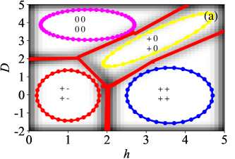
According to Refs. [20, 14], in the low-temperature regime, the BC model exhibits four distinct phases. These phases have been classified based on their similarity degree, given by $P_{1}(\begin{smallmatrix}+-\\ +-\end{smallmatrix})$, $P_{2}(\begin{smallmatrix}+0\\ +0\end{smallmatrix})$, $P_{3}(\begin{smallmatrix}++\\ ++\end{smallmatrix})$, and $P_{4}(\begin{smallmatrix}00\\ 00\end{smallmatrix})$, which are shown on the rightmost column of Fig. 3.

In Fig. 5 (a), the image energy (gray color) is obtained as

$$E(D,h)=-\sum_{i}|\frac{\partial P_{i}(D,h)}{\partial D}|^{2}-|\frac{\partial P_{i}(D,h)}{\partial h}|^{2}.$$ (11)

The four circular or elliptical contours denote the initial active contours, which move towards the boundary marked by the red solid lines under the influence of both image forces and internal forces [22, 14].

The scattering plot of the two-times clustering is also shown in Fig. 5 (b). The corresponding relations between each cluster and configuration are as follows, i.e., a $\begin{smallmatrix}++\\ ++\end{smallmatrix}$, b $\begin{smallmatrix}--\\ --\end{smallmatrix}$, c $\begin{smallmatrix}-+\\ -+\end{smallmatrix}$, d $\begin{smallmatrix}0+\\ 0+\end{smallmatrix}$, e $\begin{smallmatrix}+-\\ +-\end{smallmatrix}$ and f $\begin{smallmatrix}+0\\ +0\end{smallmatrix}$. Finally, by the similarity test as explained in Fig. 2, the cluster c $\begin{smallmatrix}-+\\ -+\end{smallmatrix}$ and e $\begin{smallmatrix}+-\\ +-\end{smallmatrix}$ are overlapped and assigned with the same label. Similarly, d $\begin{smallmatrix}0+\\ 0+\end{smallmatrix}$ and f $\begin{smallmatrix}+0\\ +0\end{smallmatrix}$ are assigned with the same labels.

Looking closely at Fig. 5 (b), the scatter plot is symmetric about the $\lambda_{1}=0$ axis due to the degenerate states. These symmetrical patterns appear in diagrams in the Ref. [3, 16], where the scattering of the generated ordered states ++++ and - - - - of the Ising model are also distributed symmetrically. Here we use the similarity test to consider them as the same phase although they are separated in the scattering plot.

In principle, the phase behavior of the BC model can be obtained using the XNOR kernel method, where the 2*2 small blocks are in the perfect configuration as kernels. In the neural network approach, the perfect configurations and their labels are used to train the kernel matrix. The common goal is to obtain the similarity, but the XNOR method is simpler and easier to understand, and the neural network method is easier to extract the features of a large amount of data. It is important to emphasize that in the neural network approach, the ”labels” are obtained through secondary clustering, and they are unknown in advance. The method proposed in this paper is an unsupervised machine learning method.

III.2.2 Three-dimensional phase diagram

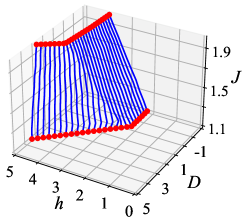
In the Blume-Capel model, $J$ is a new variable introduced to form a three-dimensional phase diagram with $D$-$h$-$J$ as the three variables. However, to train the neural network, the 3D phase diagram is technically cut into 10 two-dimensional phase diagrams, $D$-$h$-$J_{i}$, where $J_{i}$ ranges between 1 and 2 in intervals of 0.1. As shown in Fig. 6, the phase boundary of the $\begin{smallmatrix}++++\end{smallmatrix}$ state shifts as $J$ varies.

Despite training with only one two-dimensional phase diagram, the neural network is able to generalize and accurately predict and classify all of the phase diagram data in the 10 two-dimensional plots. This is likely due to the fact that the patterns and structures of the phase diagram are similar across all values of $J$.

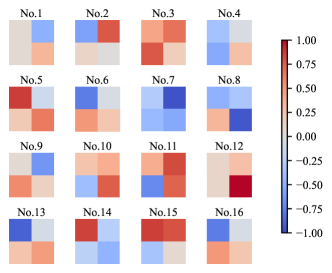
The neural network trained using the perfect configuration obtained by two-times clustering can predict the phase diagrams corresponding to different $J$, and this is related to the fitting ability of the neural network. Fig. 7 shows the convolution kernels. The various pattern is rich and exceeds the artificially defined ones. Unfortunately, clear interpretability is missing. The data range of the kernel is almost symmetric, varying from -1 to 1, perhaps related to the potential symmetry of the Hamiltonian or the spin variables of the BC model.

Figure 6: The three-dimensional phase transition boundary of the phase $\begin{smallmatrix}++\\ ++\end{smallmatrix}$.

Figure 7: Convolution kernels learned in the neural network.

IV Conclusion and Discussion

In this paper, we propose a two-times clustering method to select perfect configurations from a range of degenerate samples. We use these configurations to train a neural network for the classification of two-dimensional phase diagram data and for identifying phase boundaries. If we don’t use our two-times clustering method, some dimensionality reduction algorithms may consider ++++ and - - - - ordered configurations as two separate phases and label them differently.

We provide an example of the nearest-neighbor interaction Ising model or Potts model, where the temperature induces a phase transition from a ferromagnetic to a paramagnetic phase. Here, no two-times clustering is necessary to determine the phase transition point. However, for more complex systems like the BC model containing rich phases, we need a two-times clustering method to select the perfect configurations and assign them the labels.

While similar to using the Hamming distance to locate phase transition points in the literature [23], this paper’s primary focus is on two-times clustering to identify perfect configurations and assign the correct labels. Prior studies, such as Refs. [17], used theoretical ground state configurations in ordered phases as a training set for neural networks. For more complex systems, employing methods such as two-times clustering to identify perfect configurations is an alternative. Notably, we incorporate physics in the clustering center selection process, whereby the samples in the clustering centers correspond to the lowest energy.

In the future, we plan to test the robustness of the two-times clustering method by including examples such as frustrated lattices [24], quantum interacting bose-Hubbard systems [25, 26], topological systems [18], and real material experiments.

Acknowledgements: We thank Lan Xinfei, Wang Xinzhu, Wang Yulin, Sun Xiaodong, and Ma Heyang for their assistance in this research. We gratefully acknowledge the support of the Hefei National Research Center for Physical Sciences at the Microscale (KF2021002) for this work.

References

- Carrasquilla and Melko [2017] J. Carrasquilla and R. G. Melko, Machine learning phases of matter, Nat. Phys. 13, 431 (2017).
- Carleo et al. [2019] G. Carleo, I. Cirac, K. Cranmer, L. Daudet, M. Schuld, N. Tishby, L. Vogt-Maranto, and L. Zdeborová, Machine learning and the physical sciences, Rev. Mod. Phys. 91, 045002 (2019).
- Wang [2016] L. Wang, Discovering phase transitions with unsupervised learning, Phys. Rev. B 94, 195105 (2016).
- Wetzel [2017] S. J. Wetzel, Unsupervised learning of phase transitions: From principal component analysis to variational autoencoders, Phys. Rev. E 96, 022140 (2017).
- Hu et al. [2017] W. Hu, R. R. P. Singh, and R. T. Scalettar, Discovering phases, phase transitions, and crossovers through unsupervised machine learning: A critical examination, Phys. Rev. E 95, 062122 (2017).
- Ch’ng et al. [2018] K. Ch’ng, N. Vazquez, and E. Khatami, Unsupervised machine learning account of magnetic transitions in the hubbard model, Phys. Rev. E 97, 013306 (2018).
- Yang et al. [2021] Y. Yang, Z.-Z. Sun, S.-J. Ran, and G. Su, Visualizing quantum phases and identifying quantum phase transitions by nonlinear dimensional reduction, Phys. Rev. B 103, 075106 (2021).
- Rodriguez-Nieva and Scheurer [2019] J. F. Rodriguez-Nieva and M. S. Scheurer, Identifying topological order through unsupervised machine learning, Nat. Phys. 15, 790 (2019).
- Scheurer and Slager [2020] M. S. Scheurer and R.-J. Slager, Unsupervised machine learning and band topology, Phys. Rev. Lett. 124, 226401 (2020).
- Lidiak and Gong [2020] A. Lidiak and Z. Gong, Unsupervised machine learning of quantum phase transitions using diffusion maps, Phys. Rev. Lett. 125, 225701 (2020).
- Wang et al. [2021a] J. Wang, W. Zhang, T. Hua, and T.-C. Wei, Unsupervised learning of topological phase transitions using the calinski-harabaz index, Phys. Rev. Research 3, 013074 (2021a).
- Van Nieuwenburg et al. [2017] E. P. L. Van Nieuwenburg, Y.-H. Liu, and S. D. Huber, Learning phase transitions by confusion, Nat. Phys. 13, 435 (2017).
- Liu and van Nieuwenburg [2018] Y.-H. Liu and E. P. L. van Nieuwenburg, Discriminative cooperative networks for detecting phase transitions, Phys. Rev. Lett. 120, 176401 (2018).
- Sun et al. [2023] X. Sun, H. Yang, N. Wu, T. C. Scott, J. Zhang, and W. Zhang, Snake net and balloon force with a neural network for detecting multiple phases (2023), arXiv:2205.09699 [cond-mat.stat-mech] .
- Caliński and Harabasz [1974] T. Caliński and J. Harabasz, A dendrite method for cluster analysis, Communications in Statistics 3, 1 (1974).
- Wang et al. [2021b] J. Wang, W. Zhang, T. Hua, and T.-C. Wei, Unsupervised learning of topological phase transitions using the calinski-harabaz index, Phys. Rev. Res. 3, 013074 (2021b).
- Li et al. [2018] C.-D. Li, D.-R. Tan, and F.-J. Jiang, Applications of neural networks to the studies of phase transitions of two-dimensional potts models, Annals of Physics 391, 312 (2018).
- Tan and Jiang [2020] D.-R. Tan and F.-J. Jiang, Machine learning phases and criticalities without using real data for training, Phys. Rev. B 102, 224434 (2020).
- Jin and Han [2010] X. Jin and J. Han, K-Means Clustering, in Encyclopedia of Machine Learning, edited by C. Sammut and G. I. Webb (Springer US, Boston, MA, 2010) pp. 563–564.
- Guerrero and Stariolo [2019] A. I. Guerrero and D. A. Stariolo, The blume-capel model in a square lattice with jx=-jy interactions in an external field, Physica A: Statistical Mechanics and its Applications 532, 121839 (2019).
- Wu [1982] F. Y. Wu, The Potts model, Rev. Mod. Phys. 54, 235 (1982).
- Kass et al. [1988] M. Kass, A. P. Witkin, and D. Terzopoulos, Snakes: Active contour models, International Journal of Computer Vision 1, 321 (1988).
- Yi et al. [2022] T.-C. Yi, R. T. Scalettar, and R. Mondaini, Hamming distance and the onset of quantum criticality, Phys. Rev. B 106, 205113 (2022).
- Ce Wang [2018] H. Z. Ce Wang, Machine learning of frustrated classical spin models (ii): Kernel principal component analysis, Frontiers of Physics 13, 130507 (2018).
- Jaksch et al. [1998] D. Jaksch, C. Bruder, J. I. Cirac, C. W. Gardiner, and P. Zoller, Cold bosonic atoms in optical lattices, Phys. Rev. Lett. 81, 3108 (1998).
- Wei et al. [2021] H. Wei, J. Zhang, S. Greschner, T. C. Scott, and W. Zhang, Quantum monte carlo study of superradiant supersolid of light in the extended jaynes-cummings-hubbard model, Phys. Rev. B 103, 184501 (2021).