General treatment of Gaussian trusted noise
in continuous variable quantum key distribution

Abstract

Continuous Variable (CV) quantum key distribution (QKD) is a promising candidate for practical implementations due to its compatibility with the existing communication technology. A trusted device scenario assuming that an adversary has no access to imperfections such as electronic noises in the detector is expected to provide significant improvement in the key rate, but such an endeavor so far was made separately for specific protocols and for specific proof techniques. Here, we develop a simple and general treatment that can incorporate the effects of Gaussian trusted noises for any protocol that uses homodyne/heterodyne measurements. In our method, a rescaling of the outcome of a noisy homodyne/heterodyne detector renders it equivalent to the outcome of a noiseless detector with a tiny additional loss, thanks to a noise-loss equivalence well-known in quantum optics. Since this method is independent of protocols and security proofs, it is applicable to Gaussian-modulation and discrete-modulation protocols, to the finite-size regime, and to any proof techniques developed so far and yet to be discovered as well.

I Introduction

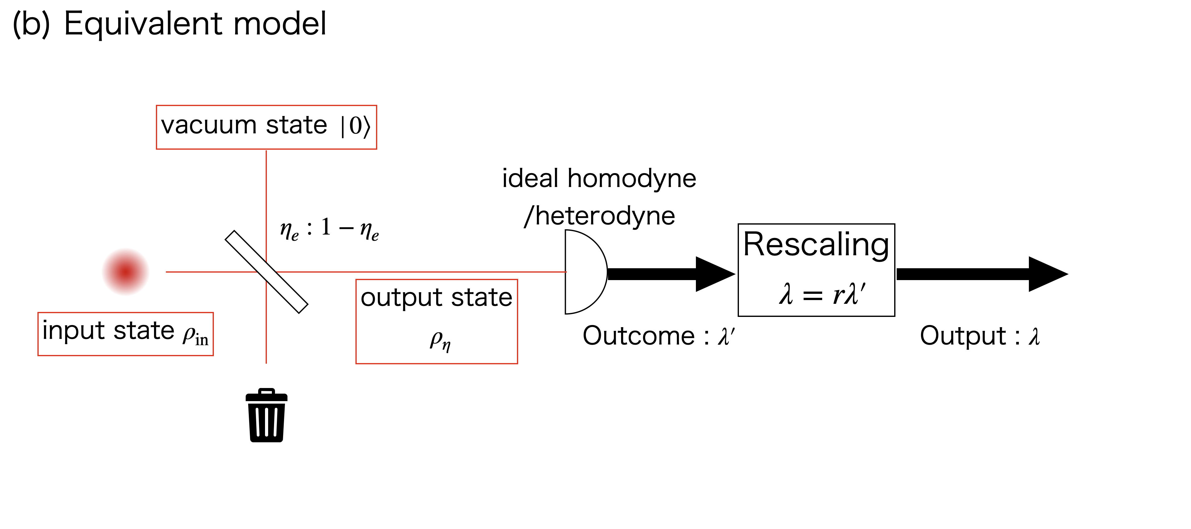
Figure 1: (a) Trusted device model of a noisy measurement in CV QKD. (b) Measurement model equivalent to (a).

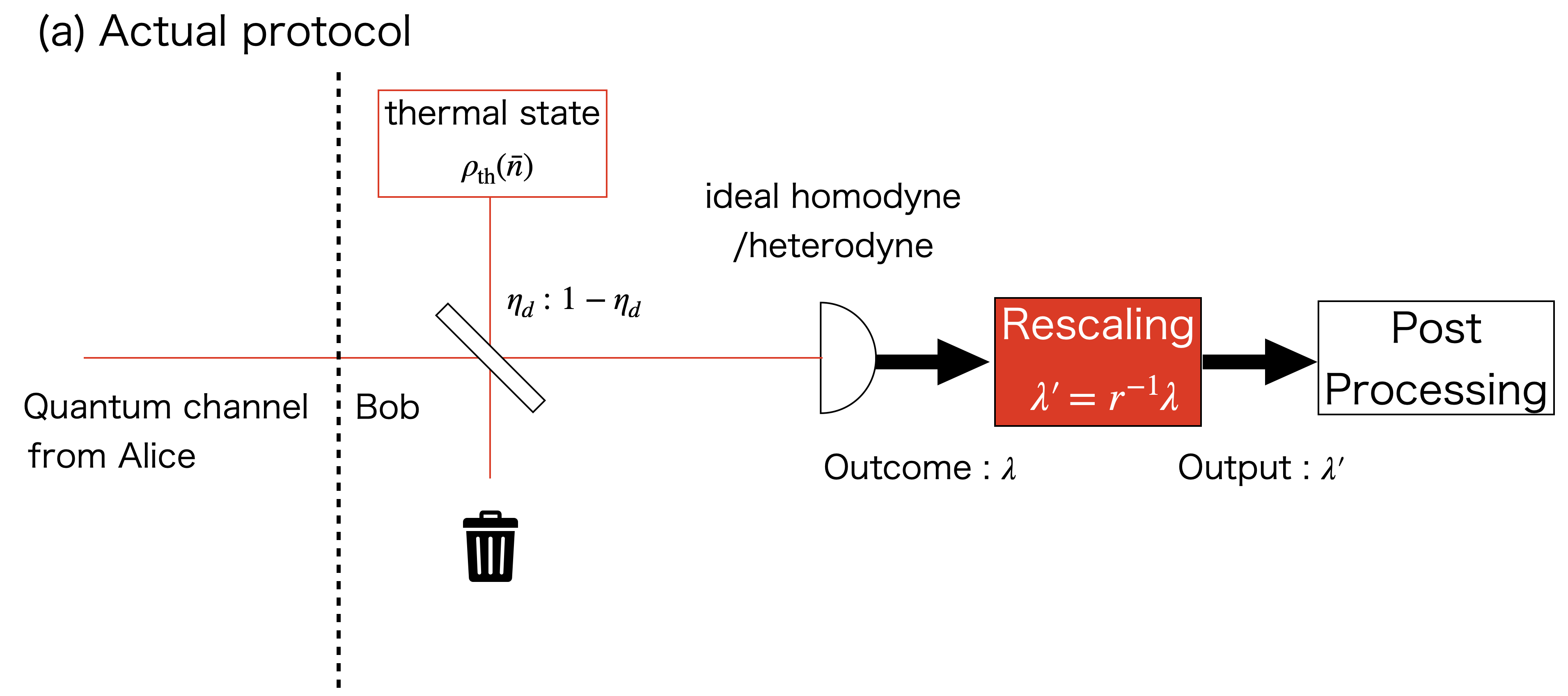
Figure 2: (a) Actual protocol with a noisy measurement followed by rescaling. (b) Equivalent protocol with a noiseless measurement.

Quantum key distribution (QKD) is the technology that enables information-theoretically secure communication between two separate parties. QKD is classified into discrete-variable (DV) QKD and continuous-variable (CV) QKD. It is customary to make the classification according to detection methods in the receiver, regardless of encoding methods in the transmitter. DV-QKD protocols use photon detectors to read out the encoded information. The early proposals [1, 2] of QKD belong to this type, and much knowledge about finite-key analysis and how to handle imperfections of actual devices has been accumulated. On the other hand, CV-QKD protocols use homodyne or heterodyne detection [3, 4], which is highly compatible with the coherent optical communication technology currently widespread in the industry [5, 6, 7, 8, 9, 10, 11, 12].

In actual experiments, the state sent by the sender Alice is not directly transmitted to the receiver Bob, but the state is affected by noises and losses in the quantum channel and their devices. As for the noises and losses that occurred in the quantum channel, Alice and Bob cannot distinguish whether they are caused by the eavesdropper Eve’s attack. One must then assume that they are all caused by Eve in calculating an appropriate amount of privacy amplification. On the other hand, since the detector is physically protected in Bob’s lab, it is often reasonable to assume that Eve has no access to imperfections in the detector [13]. The security under this relaxed assumption has been considered in the past and is called a trusted device scenario (see review [14]). Especially for homodyne/heterodyne measurements used in CV-QKD, where the classical noise of the electronic circuit after the detection is often larger than the excess noise of the channel, the trusted device assumption can significantly improve the key rate of a QKD protocol [15, 16, 17, 18, 19, 20].

From a theoretical point of view, it is crucial to find quantitative relations between the parameters describing the amount of trusted noises and the reduction in the amount of privacy amplification by assessing how the trusted device scenario limits the amount of information leaked to Eve. So far, such an endeavor was made separately for specific protocols and for specific proof techniques. In Gaussian modulation schemes, since it was proved that the optimal attack for Eve is the entangling cloner attack, it is relatively easy to evaluate the effect of Gaussian trusted noises by computing the covariance matrix of a quantum state before it incurred the trusted noises [21, 22, 23, 24, 25, 26, 13, 27, 28]. As for discrete modulation protocols, Namiki et al.[29] adopted an assumption that limits Eve’s attacks to the entangling cloner attacks and determined the amount of privacy amplification for Gaussian noises. Lin and Lütkenhaus [30] relaxed the assumption to collective attacks in the case of a specific proof technique based on numerical optimization. Currently, there are many different approaches [31, 32, 33] to the finite-size security against general attacks on CV-QKD, but the trusted device scenario for these approaches has not been explicitly given. Mere extension of existing methods would require a separate argument for each of the finite-size approaches.

In this study, we develop a simple and general treatment that can incorporate the effects of Gaussian trusted noises for any protocol that applies homodyne/heterodyne measurements. Specifically, we introduce a rescaling of the outcome of a noisy homodyne/heterodyne detector which renders it equivalent to a noiseless detector with a tiny additional loss, thanks to the noise-loss equivalence well-known in quantum optics. Since this method is independent of protocols and security proofs, it is applicable to Gaussian-modulation and discrete modulation protocols, to asymptotic and finite-sized regimes, and to any proof techniques developed so far and yet to be discovered as well.

This paper is organized as follows. In Sec. II, we introduce an equivalent model of the noisy measurement in the trusted device scenario and explain a method for treating trusted Gaussian noises for homodyne/heterodyne detection. In Sec. III, we specifically apply our method to the binary modulation protocol and show numerical simulations of the key rates. We conclude this paper in Sec. IV.

II METHODS

The main imperfection in the homodyne/heterodyne measurement device is its non-unit quantum efficiency and noises on the electronic circuit. As in the previous analyses on the trusted noises, we assume that the noises are Gaussian, and that the imperfect homodyne/heterodyne measurement is equivalently represented by a quantum optical model shown in Fig. 2 (a). In this model, the input optical pulse is mixed with an ancillary pulse $R$ that is in a thermal state with an average photon number $\bar{n}$ by a beam splitter with a transmittance $\eta_{d}$, and then is fed to an ideal homodyne/heterodyne detector to produce an outcome $\lambda\in\Omega$ ($\Omega=\mathbb{R}$ for homodyne and $\Omega=\mathbb{C}$ for heterodyne). In the trusted device scenario, we assume that Eve has no access to the device and hence the thermal ancillary pulse and Eve’s system are decoupled.

Let $\rho$ be the state of the input pulse and $\rho_{\rm noisy}$ be the state of the pulse just before the ideal homodyne/heterodyne detector. The completely positive and trace preserving (CPTP) map $\mathcal{E}$ for the mixing of the thermal light is represented by

$$\rho_{\rm noisy}=\mathcal{E}(\rho)={\rm Tr}_{R}\left[S(\eta_{d})\rho\otimes\rho_{\rm th}(\bar{n})S^{\dagger}(\eta_{d})\right],$$ (1)

where $\rho_{\rm th}(\bar{n})$ is a thermal state with the mean photon number $\bar{n}$ and $S(\eta)$ is the unitary operator for the beamsplitter with transmittance $\eta$ . Let us denote the positive-operator-valued measure (POVM) for the ideal homodyne/heterodyne detector as $\Pi(\Delta)(\Delta\subset\Omega)$. The POVM $\Pi_{\rm noisy}(\Delta)$ of the noisy homodyne/heterodyne measurement modeled in Fig. 2 (a) is then given by

$$\Pi_{\rm noisy}(\Delta)=\mathcal{E}^{\dagger}(\Pi(\Delta)).$$ (2)

where $\mathcal{E}^{\dagger}$ is the adjoint map of $\mathcal{E}$.

Next, we consider another model shown in Fig. 2 (b), which will be shown to be equivalent to the one in Fig. 2 (a). Here, the input light pulse is mixed with the vacuum state $\ket{0}$ using a beamsplitter with a transmittance $\eta_{e}$ and is then fed to the same homodyne/heterodye detector to produce an intermediate outcome $\lambda^{\prime}\in\Omega$. It is then rescaled by a factor $r\geq 1$ to produce a final outcome $\lambda=r\lambda^{\prime}$. Let $\rho_{\eta_{e}}$ be the state of the pulse just before the ideal homodyne/heterodyne detector. The CPTP map for converting $\rho$ to $\rho_{\eta_{e}}$ is then given by

$$\rho_{\eta_{e}}=\mathcal{E}_{\rm eq}(\rho)={\rm Tr}_{R}\left[S(\eta_{e})\rho\otimes\ket{0}\bra{0}_{R}S^{\dagger}(\eta_{e})\right].$$ (3)

The POVM $\Pi_{\rm eq}(\Delta)$ of the measurement modeled in Fig. 2 (b) is then given by

$$\Pi_{\rm eq}(\Delta)=\mathcal{E}_{\rm eq}^{\dagger}(\Pi(r^{-1}(\Delta))),$$ (4)

where $r^{-1}(\Delta)=\{\lambda^{\prime}|r\lambda^{\prime}\in\Delta\}$. The measurement model in Fig. 2 (b) can be made equivalent to the one in Fig. 2 (a) by appropriately choosing $\eta_{e}$ and $r$. We will prove in Appendix A, B that $\Pi_{\rm noisy}(\Delta)=\Pi_{\rm eq}(\Delta)$ holds when

$$r^{2} =1+2\bar{n}(1-\eta_{d})$$ (5)

$$\eta_{e} =r^{-2}\eta_{d}.$$ (6)

for a homodyne measurement, and when

$$r^{2} =1+\bar{n}(1-\eta_{d})$$ (7)

$$\eta_{e} =r^{-2}\eta_{d}.$$ (8)

for a heterodyne measurement.

Our general method for trusted Gaussian noises is stated as follows. Whenever a QKD protocol dictates to use an outcome $\lambda$ of a homodyne/heterodyne detector, we modify it to use its rescaled value $\lambda^{\prime}=r^{-1}\lambda$ instead of $\lambda$. If the parameter $r$ is chosen according to the parameters $(\eta_{d},\bar{n})$ of the trusted noises of the detector, this modified protocol in Fig. 2 (a) is equivalent to the one in Fig. 2 (b). This enables us to use any security proof assuming noiseless detector with a slightly increased loss $\eta_{e}=r^{-2}\eta_{d}$ to determine a sufficient amount of privacy amplification.

When a CV QKD protocol uses two or more homodyne/heterodyne detectors, the above method may not work as it is, because security proofs often assume that different detectors have the same quantum efficiency. For example, a security proof is first constructed assuming ideal homodyne/heterodyne detectors, and then is claimed to be applicable to the case with inefficient (but noiseless) detectors with the same quantum efficiency, on the basis that the common loss can be ascribed to Eve’s attack.

Fortunately, there are several remedies at the implementation level. Since the reduced efficiency $\eta_{e}$ is a function of original loss $\eta_{d}$ and noise $\bar{n}$, one may introduce an additional loss or noise to a detector to decrease its reduced efficiency $\eta_{e}$. For an additional loss, one may directly insert a lossy component or may intentionally worsen the spatial mode matching between the signal and LO. For an additional noise, one may use random-number generator to add a Gaussian noise to the outcome, or may just reduce the LO power if the original noise is in the photodetector and the subsequent circuits. Given the worst value $\eta_{e}^{\rm(min)}$ among the detectors, one can thus make all the detectors have the reduced efficiency $\eta_{e}^{\rm(min)}$ in this way.

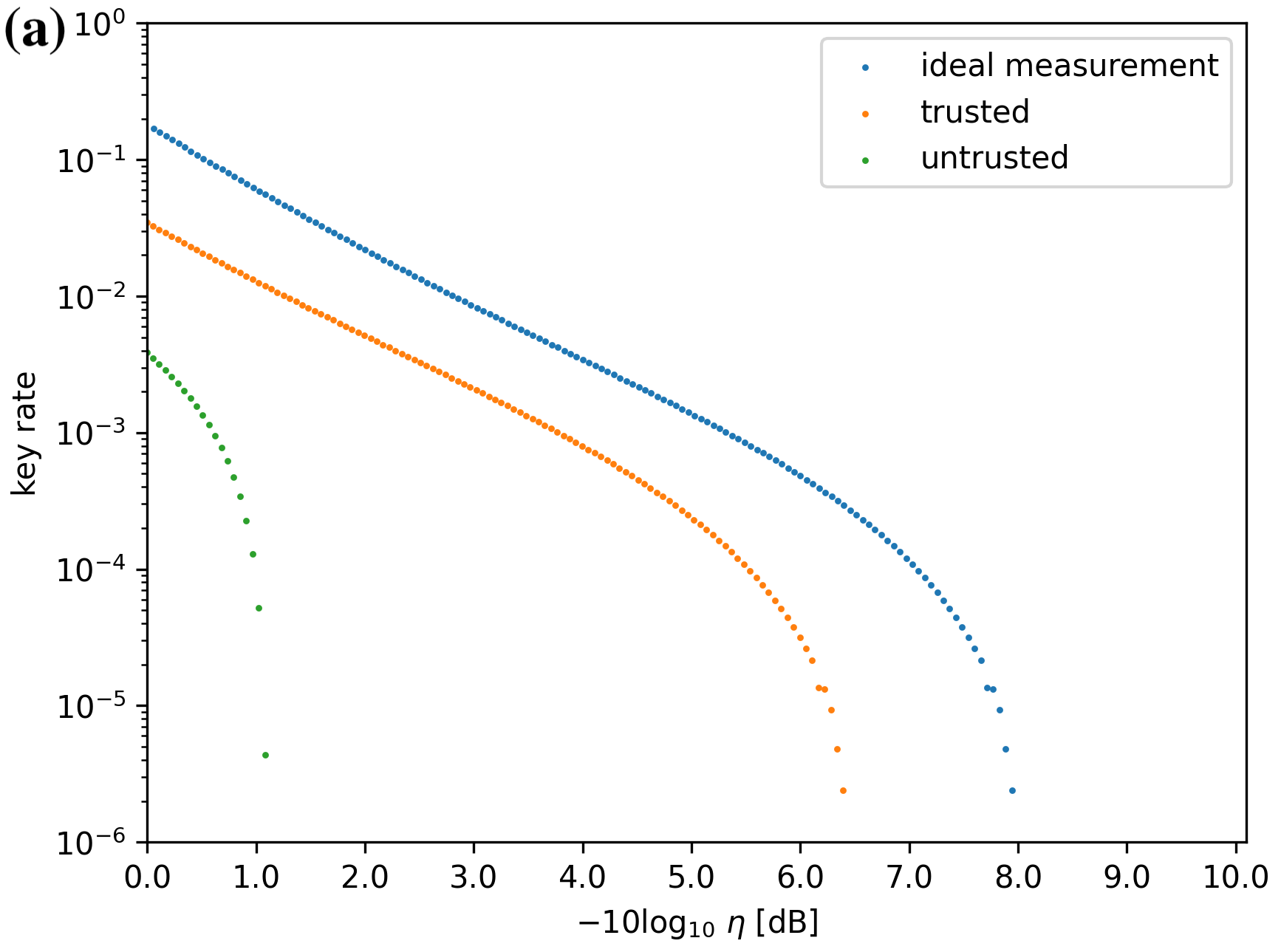
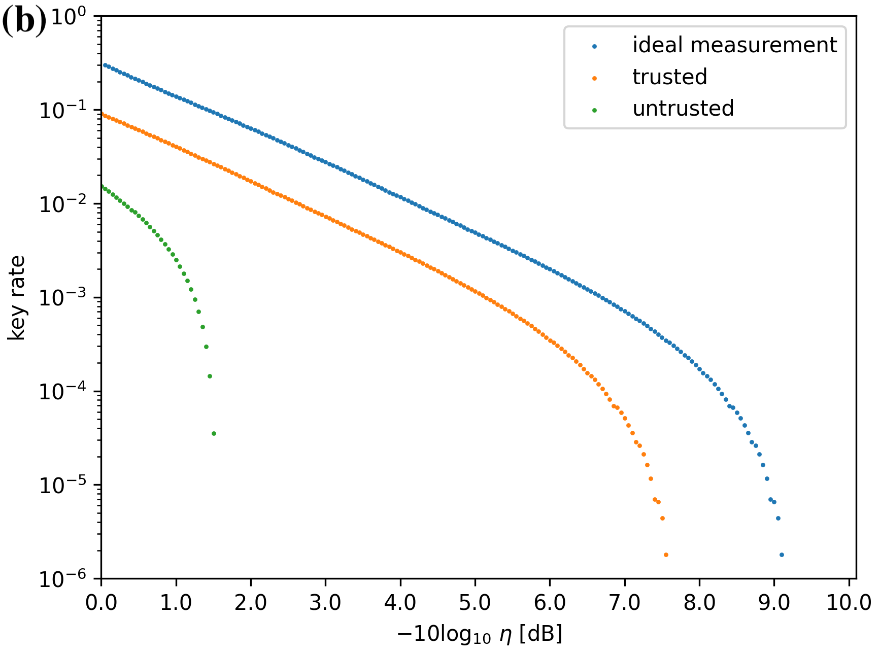
Figure 3: The key rate comparison for the the cases where the detector is ideal, has trusted noises, and has untrusted noises. (a) Protocol with heterodyne measurement. (b) Protocol with homodyne and heterodyne measurements.

III Example

As an example, we apply this method to two variants of reverse reconciliation protocols with binary modulation [34]. Two variants of protocols were analyzed in Ref. [34], an all-heterodyne protocol and a hybrid protocol using both homodyne and heterodyne measurements. For both protocols, the security proof covers the finite-key-size regime against general coherent attacks. For this protocol, the conventional treatment of the trusted noise[21, 22, 23, 24, 25, 26, 13, 27, 28] does not work since it does not use the property of the covariance matrix.

For the simulation of the key rate, we set the security parameter $\epsilon_{\rm sec}=2^{-50}$ and the communication channel as follows. We assume the communication channel to be a phase-invariant Gaussian channel with the transmittance $\eta$ and excess noise $\xi$. We assume that the noise is ascribed to a fixed noise source at the input with $\xi_{0}=10^{-3}$, which means the excess noise is given by $\xi=\eta\xi_{0}$. This quantum channel can be modeled by random displacement followed by a pure loss channel. Under this model, a coherent state $\ket{\beta}$, after transmitted through this quantum channel, becomes

$$\rho_{\rm in}=\frac{1}{\eta\xi_{0}}\int_{\mathbb{C}}\frac{2}{\pi}\exp\left(-\frac{2|\gamma|^{2}}{\eta\xi_{0}}\right)\ket{\sqrt{\eta}\beta+\gamma}\bra{\sqrt{\eta}\beta+\gamma}d^{2}\gamma.$$ (9)

For the all-heterodyne protocol, we assume that the heterodyne detector has a quantum efficiency $\eta_{d}=0.7=1.5$\mathrm{dB}$$ and noise $2\bar{n}(1-\eta_{d})=10^{-3}$ and simulated the finite-size key rates with $10^{12}$ transmitted pulses. In the trusted noise scenario, our method gives $r^{2}=1+0.5\times 10^{-3}$ and the key rate is the same as the case with a Gaussian channel with transmittance $\eta\eta_{e}=\eta\eta_{d}r^{-2}$ and excess noise $\eta\eta_{e}\xi_{0}$ followed by an ideal detector, which can be calculated using the formula in Ref. [34] and is shown as the curve labeled as “trusted” in Fig. 3 (a). If we do not use the trusted scenario and ascribe all the imperfection to the quantum channel, it becomes a Gaussian channel with transmittance $\eta\eta_{d}$ and excess noise $\eta\eta_{d}\xi_{0}+10^{-3}$. This rate is shown as the curve labeled as “untrusted” in Fig. 3 (a). We also show the key rate when the ideal detector ($\eta_{d}=\bar{n}=0$) is used. We see that the trusted-device scenario significantly improves the key rate compared to the untrusted one, to the extent that the effect of the noises is almost eliminated.

For the hybrid protocol, we consider the case where both of the detectors have the same quantum efficiency $\eta_{d}=0.7=1.5$\mathrm{dB}$$ and the same noise parameter $2\bar{n}(1-\eta_{d})=10^{-3}$. Then the rate with the untrusted case is again given by considering a quantum channel made up of a Gaussian channel with transmittance $\eta\eta_{d}$ and excess noise $\eta\eta_{d}\xi_{0}+10^{-3}$. For the trusted scenario, the reduced efficiency differs for the two detectors: $\eta_{e}=\eta_{d}/(1+10^{-3})$ for the homodyne detector and $\eta_{e}=\eta_{d}/(1+0.5\times 10^{-3})$ for the heterodyne detector. Hence our method is applicable after an additional loss or noises are introduced such that its reduced efficiency becomes $\eta_{e}^{\rm(min)}=\eta_{d}/(1+10^{-3})$. The key rate is then given as the case with a Gaussian channel with transmittance $\eta\eta_{e}^{\rm(min)}$ and excess noise $\eta\eta_{e}^{\rm(min)}\xi_{0}$ followed by an ideal detector. The result is shown in Fig. 3 (b), which shows almost the same tendency as Fig. 3 (a).

IV discussion and conclusion

As shown in Fig. 3, in both the homodyne and hybrid protocols, the difference between an ideal detector and a detector with trusted noise is essentially only in the detection efficiency. This behavior can be understood in the general terms as follows. The noise-loss equivalence in a homodyne/heterodyne measurement trades an excess noise $\xi$ with an additional loss of $O(\xi)$. Under this equivalence, the performance of the CV-QKD is affected by the two types of imperfections in an extremely asymmetric way, namely, it is vulnerable against noise but robust against loss. This is the reason why the trusted noise scenario remarkably improves the key rate of CV-QKD.

It is worth mentioning that assuming the device model of Fig. 2 (a) with parameters $\eta_{d}$ and $\bar{n}$ does not necessarily require the characterization of the actual detector for the two parameters. It is often the case that a QKD protocol (including the computation of the amount of privacy amplification) does not use the value of $\eta_{d}$. In such a case, the only value required in constructing the Actual protocol in Fig. 2 (a) in our method is $\bar{n}(1-\eta_{d})$. Characterization of this value is achieved by inputting a vacuum state into the device and measuring the variance of its quadrature.

There is also a minor but frequent issue in the model of Fig. 2 (a). In QKD, it is customary to model the actual detector by a pure-loss channel followed by a detector with $\eta_{d}=1$ while the channel is assumed to be in Eve’s control. It is preferred (i) when an available security proof assumes a detector with perfect efficiency, or (ii) when the apparent loss in the detector cannot be trusted and Eve may suppress it. In either case, there are cases when we can reasonably trust the noises in the detector, such as the electrical noises. A problem in applying our method of trusted scenario is that the model of Fig. 2 (a) with $\eta_{d}=1$ cannot represent nonzero noises. The remedy here is to represent a noisy detector with $\eta_{d}=1$ by a limit of a sequence of models of Fig. 2 (a) with a fixed value of $\bar{n}(1-\eta_{d})$ and $\eta_{d}\to 1$. This allows the computation of $r$ and $\eta_{e}$ to apply our method.

In conclusion, we propose a simple method to treat Gaussian noise in the trusted device scenario. By introducing a slight modification in the actual protocol such that one uses rescaled values of quadrature outcomes of the noisy detectors, we can benefit from a device-level equivalence to noiseless detectors with a tiny additional loss. CV-QKD protocols tend to be vulnerable to noise, and it has been suggested that the trusted device scenario for the receiver markedly improves the key rates. Our contribution is to widen its applicability considerably without regard to protocols and proof techniques. We numerically confirmed for specific protocols with finite-size security proofs that the trusted device scenario almost entirely mitigates the effect of the detector noise. Since our method has a simple effect of trading the Gaussian detector noise with a tiny loss, we expect a similar benefit from any CV-QKD protocol with the trusted device scenario.

Appendix A homodyne measurement

We introduce the annihilation operator $\hat{a}$ and creation operator $\hat{a}^{\dagger}$ of a single-mode state with the usual commutation relation $[\hat{a},\hat{a}^{\dagger}]=1$, and define the quadrature operator:

$$\hat{x} =\frac{1}{2}(\hat{a}+\hat{a}^{\dagger})$$ (10)

$$\hat{p} =\frac{i}{2}(\hat{a}-\hat{a}^{\dagger}).$$ (11)

The coherent state $\ket{\alpha}$ is written as

$$\ket{\alpha}=e^{-\frac{|\alpha|^{2}}{2}}\sum_{n=0}^{\infty}\frac{\alpha^{n}}{\sqrt{n!}}\ket{n},$$ (12)

and the wave function $\braket{x}{\alpha}$ is

$$\braket{x}{\alpha}=\left(\frac{2}{\pi}\right)^{\frac{1}{4}}\exp[-(x-\alpha_{R})^{2}+2i\alpha_{I}x-i\alpha_{R}\alpha_{I}],$$ (13)

where $\alpha_{R}={\rm Re}(\alpha),\alpha_{I}={\rm Im}(\alpha)$. The density operator of the thermal state with mean photon number $\bar{n}$ is described as

$$\rho_{\rm th}(\bar{n}) =\sum_{n=0}^{\infty}\frac{\bar{n}^{n}}{(1+\bar{n})^{n+1}}\ket{n}\bra{n}$$ (14)

$$=\frac{1}{\pi\bar{n}}\int_{\mathbb{C}}\exp(-\frac{|\beta|^{2}}{\bar{n}})\ket{\beta}\bra{\beta}d^{2}\beta.$$ (15)

The condition for two POVMs to be equal is that their probability distributions are equal for any coherent states [35]. Then, we consider the coherent state $\rho_{\rm in}=\ket{\alpha}\bra{\alpha}$ as input. In the trusted device model, the state to which Bob performs the ideal measurement is calculated as

$$\mathcal{E}(\rho_{\rm in}) =\rho_{\rm noisy}$$ (16)

$$={\rm Tr}_{R}\left[S(\eta_{d})\ket{\alpha}\bra{\alpha}\otimes\rho_{\rm th}(\bar{n})S^{\dagger}(\eta_{d})\right]$$ (17)

$$=\frac{1}{\pi}\int\frac{1}{\bar{n}}\exp\left(-\frac{|\beta|^{2}}{\bar{n}}\right)$$

$$\ket{\sqrt{\eta_{d}}\alpha+\sqrt{1-\eta_{d}}\beta}\bra{\sqrt{\eta_{d}}\alpha+\sqrt{1-\eta_{d}}\beta}d^{2}\beta,$$ (18)

and in the equivalent model, Bob measures the state $\mathcal{E}_{\rm eq}(\rho_{\rm in})=\rho_{\eta_{e}}=\ket{\sqrt{\eta_{e}}\alpha}\bra{\sqrt{\eta_{e}}\alpha}$.

The homodyne measurement outputs a real number $x\in\mathbb{R}$. The probability density of an outcome $x$ of an ideal homodyne measurement with an input state $\rho$ is given by $\braket{x}{\rho}{x}$. The probability distribution obtained by the trusted device model ${\rm Pr}\left(x\in\Delta\right)$ is written as

$${\rm Tr}(\rho_{\rm in}\Pi_{\rm noisy}(\Delta))$$ (19)

$$= {\rm Tr}(\mathcal{E}(\rho_{\rm in})\Pi(\Delta))$$ (20)

$$= \int_{x\in\Delta}\bra{x}\mathcal{E}(\rho_{\rm in})\ket{x}dx$$ (21)

$$= \int_{x\in\Delta}\frac{1}{\sqrt{2\pi\sigma^{2}_{\rm hom}}}\exp(-\frac{(x-\sqrt{\eta_{d}}x_{0})^{2}}{2\sigma^{2}_{\rm hom}})dx,$$ (22)

where we defined $x_{0}={\rm Re}(\alpha)$ and

$$\sigma^{2}_{\rm hom} =\frac{1+2\bar{n}(1-\eta_{d})}{4}.$$ (23)

Then, in the equivalent model, the probability distribution is given by

$${\rm Tr}(\rho_{\rm in}\Pi_{\rm eq}(\Delta))$$ (24)

$$= {\rm Tr}(\mathcal{E}_{\rm eq}(\rho_{\rm in})\Pi(r^{-1}(\Delta)))$$ (25)

$$= \int_{x^{\prime}\in r^{-1}(\Delta)}\bra{x^{\prime}}\mathcal{E}_{\rm eq}(\rho_{\rm in})\ket{x^{\prime}}dx^{\prime}$$ (26)

$$= \int_{x\in\Delta}\bra{r^{-1}x}\mathcal{E}_{\rm eq}(\rho_{\rm in})\ket{r^{-1}x}r^{-1}dx$$ (27)

$$= \int_{x\in\Delta}\frac{1}{\sqrt{2\pi\frac{r^{2}}{4}}}\exp(-\frac{(x-r\sqrt{\eta_{e}}x_{0})^{2}}{2\times\frac{r^{2}}{4}})dx.$$ (28)

Therefore, the condition for two models to be equivalent is

$$r^{2} =1+2\bar{n}(1-\eta_{d}),$$ (29)

$$\eta_{e} =r^{-2}\eta_{d}.$$ (30)

Appendix B heterodyne measurement

The heterodyne measurement outputs a complex number $\omega\in\mathbb{C}$. The probability density of an outcome $\omega$ of an ideal heterodyne measurement with an input state $\rho$ is given by $\frac{\braket{\omega}{\rho}{\omega}}{\pi}$. The probability distribution obtained by the trusted device model ${\rm Pr}\left(\omega\in\Delta\right)$ is written as

$${\rm Tr}(\rho_{\rm in}\Pi_{\rm noisy}(\Delta)) ={\rm Tr}(\mathcal{E}(\rho_{\rm in})\Pi(\Delta))$$ (31)

$$=\int_{\omega\in\Delta}\bra{\omega}\mathcal{E}(\rho_{\rm in})\ket{\omega}\frac{d^{2}\omega}{\pi}$$ (32)

$$=\int_{\omega\in\Delta}\frac{1}{2\pi\sigma^{2}_{\rm het}}\exp(-\frac{(\omega_{R}-\sqrt{\eta_{d}}x_{0})^{2}+(\omega_{I}-\sqrt{\eta_{d}}p_{0})^{2}}{2\sigma^{2}_{\rm het}})d^{2}\omega$$ (33)

where we defined $\omega_{R}={\rm Re}(\omega)$, $\omega_{I}={\rm Im}(\omega)$, $p_{0}={\rm Im}(\alpha)$, and

$$\sigma^{2}_{\rm het} =\frac{1+\bar{n}(1-\eta_{d})}{2}.$$ (34)

Then, in the equivalent model, the probability distribution is given by

$${\rm Tr}(\rho_{\rm in}\Pi_{\rm eq}(\Delta))$$ (35)

$$= {\rm Tr}(\mathcal{E}_{\rm eq}(\rho_{\rm in})\Pi(r^{-1}(\Delta)))$$ (36)

$$= \int_{\omega^{\prime}\in r^{-1}(\Delta)}\bra{\omega^{\prime}}\mathcal{E}_{\rm eq}(\rho_{\rm in})\ket{\omega^{\prime}}\frac{d^{2}\omega^{\prime}}{\pi}$$ (37)

$$= \int_{\omega\in\Delta}\bra{r^{-1}\omega}\mathcal{E}_{\rm eq}(\rho_{\rm in})\ket{r^{-1}\omega}\frac{d^{2}\omega}{r^{2}\pi}$$ (38)

$$= \int_{\omega\in\Delta}\frac{1}{2\pi\frac{r^{2}}{2}}\exp(-\frac{(x-r\sqrt{\eta_{e}}x_{0})^{2}}{2\times\frac{r^{2}}{2}})d^{2}\omega$$ (39)

Therefore, the condition for two models to be equivalent is

$$r^{2} =1+\bar{n}(1-\eta_{d})$$ (40)

$$\eta_{e} =r^{-2}\eta_{d}.$$ (41)

References

- Bennett and Brassard [1984] C. H. Bennett and G. Brassard, Quantum cryptography : Public key distribution and coin tossing, in Proceedings of IEEE International Conference on Computers, Systems, and Signal Processing (1984) pp. 175–179.
- Bennett [1992] C. H. Bennett, Quantum cryptography using any two nonorthogonal states, Phys. Rev. Lett. 68, 3121 (1992).
- Ralph [1999] T. C. Ralph, Continuous variable quantum cryptography, Phys. Rev. A 61, 010303(R) (1999).
- Grosshans and Grangier [2002] F. Grosshans and P. Grangier, Continuous variable quantum cryptography using coherent states, Phys. Rev. Lett. 88, 057902 (2002).
- Eriksson et al. [2020] T. A. Eriksson, R. S. Luís, B. J. Puttnam, G. Rademacher, M. Fujiwara, Y. Awaji, H. Furukawa, N. Wada, M. Takeoka, and M. Sasaki, Wavelength division multiplexing of 194 continuous variable quantum key distribution channels, J. Light. Technol. 38, 2214 (2020).
- Huang et al. [2015] D. Huang, D. Lin, C. Wang, W. Liu, S. Fang, J. Peng, P. Huang, and G. Zeng, Continuous-variable quantum key distribution with 1 Mbps secure key rate, Opt. Express 23, 17511 (2015).
- Kumar et al. [2015] R. Kumar, H. Qin, and R. Alléaume, Coexistence of continuous variable QKD with intense DWDM classical channels, New J. Phys. 17, 043027 (2015).
- Huang et al. [2016a] D. Huang, P. Huang, H. Li, T. Wang, Y. Zhou, and G. Zeng, Field demonstration of a continuous-variable quantum key distribution network, Opt. Lett. 41, 3511 (2016a).
- Karinou et al. [2017] F. Karinou, L. Comandar, H. H. Brunner, D. Hillerkuss, F. Fung, S. Bettelli, S. Mikroulis, D. Wang, Q. Yi, M. Kuschnerov, C. Xie, A. Poppe, and M. Peev, Experimental evaluation of the impairments on a QKD system in a 20-channel WDM co-existence scheme, in 2017 IEEE Photonics Society Summer Topical Meeting Series (SUM) (2017) pp. 145–146.
- Karinou et al. [2018] F. Karinou, H. H. Brunner, C.-H. F. Fung, L. C. Comandar, S. Bettelli, D. Hillerkuss, M. Kuschnerov, S. Mikroulis, D. Wang, C. Xie, M. Peev, and A. Poppe, Toward the Integration of CV Quantum Key Distribution in Deployed Optical Networks, IEEE Photonics Technology Letters 30, 650 (2018).
- Eriksson et al. [2018] T. A. Eriksson, T. Hirano, M. Ono, M. Fujiwara, R. Namiki, K.-i. Yoshino, A. Tajima, M. Takeoka, and M. Sasaki, Coexistence of Continuous Variable Quantum Key Distribution and 712.5 Gbit/s Classical Channels, in 2018 IEEE Photonics Society Summer Topical Meeting Series (SUM) (2018) pp. 71–72.
- Eriksson et al. [2019] T. A. Eriksson, T. Hirano, B. J. Puttnam, G. Rademacher, R. S. Luís, M. Fujiwara, R. Namiki, Y. Awaji, M. Takeoka, N. Wada, and M. Sasaki, Wavelength division multiplexing of continuous variable quantum key distribution and 18.3 Tbit/s data channels, Commun. Phys. 2, 9 (2019).
- Pirandola [2021] S. Pirandola, Composable security for continuous variable quantum key distribution: Trust levels and practical key rates in wired and wireless networks, Phys. Rev. Res. 3, 043014 (2021).
- Usenko and Filip [2016] V. C. Usenko and R. Filip, Trusted Noise in Continuous-Variable Quantum Key Distribution: A Threat and a Defense, Entropy 18, 20 (2016).
- Lodewyck et al. [2007] J. Lodewyck, M. Bloch, R. García-Patrón, S. Fossier, E. Karpov, E. Diamanti, T. Debuisschert, N. J. Cerf, R. Tualle-Brouri, S. W. McLaughlin, and P. Grangier, Quantum key distribution over with an all-fiber continuous-variable system, Phys. Rev. A 76, 042305 (2007).
- Grosshans et al. [2003] F. Grosshans, G. Van Assche, J. Wenger, R. Brouri, N. J. Cerf, and P. Grangier, Quantum key distribution using gaussian-modulated coherent states, Nature 421, 238 (2003).
- Fossier et al. [2009] S. Fossier, E. Diamanti, T. Debuisschert, A. Villing, R. Tualle-Brouri, and P. Grangier, Field test of a continuous-variable quantum key distribution prototype, New J. Phys. 11, 045023 (2009).
- Jouguet et al. [2013] P. Jouguet, S. Kunz-Jacques, A. Leverrier, P. Grangier, and E. Diamanti, Experimental demonstration of long-distance continuous-variable quantum key distribution, Nat. Photonics 7, 378 (2013).
- Huang et al. [2016b] D. Huang, P. Huang, D. Lin, and G. Zeng, Long-distance continuous-variable quantum key distribution by controlling excess noise, Sci. Rep. 6, 19201 (2016b).
- Ren et al. [2021] S. Ren, S. Yang, A. Wonfor, I. White, and R. Penty, Demonstration of high-speed and low-complexity continuous variable quantum key distribution system with local local oscillator, Sci. Rep. 11, 9454 (2021).
- Huang et al. [2013] J.-Z. Huang, C. Weedbrook, Z.-Q. Yin, S. Wang, H.-W. Li, W. Chen, G.-C. Guo, and Z.-F. Han, Quantum hacking of a continuous-variable quantum-key-distribution system using a wavelength attack, Phys. Rev. A 87, 062329 (2013).
- Ma et al. [2014] X.-C. Ma, S.-H. Sun, M.-S. Jiang, M. Gui, Y.-L. Zhou, and L.-M. Liang, Enhancement of the security of a practical continuous-variable quantum-key-distribution system by manipulating the intensity of the local oscillator, Phys. Rev. A 89, 032310 (2014).
- Jouguet et al. [2012] P. Jouguet, S. Kunz-Jacques, E. Diamanti, and A. Leverrier, Analysis of imperfections in practical continuous-variable quantum key distribution, Phys. Rev. A 86, 032309 (2012).
- Laudenbach et al. [2018] F. Laudenbach, C. Pacher, C.-H. F. Fung, A. Poppe, M. Peev, B. Schrenk, M. Hentschel, P. Walther, and H. Hübel, Continuous-Variable Quantum Key Distribution with Gaussian Modulation―The Theory of Practical Implementations, Adv. Quantum Technol. 1, 1800011 (2018).
- Laudenbach and Pacher [2019] F. Laudenbach and C. Pacher, Analysis of the Trusted-Device Scenario in Continuous-Variable Quantum Key Distribution, Adv. Quantum Technol. 2, 1900055 (2019).
- Ren et al. [2019] S. Ren, R. Kumar, A. Wonfor, X. Tang, R. Penty, and I. White, Reference pulse attack on continuous variable quantum key distribution with local local oscillator under trusted phase noise, J. Opt. Soc. Am. B 36, B7 (2019).
- Shao et al. [2021] Y. Shao, H. Wang, Y. Pi, W. Huang, Y. Li, J. Liu, J. Yang, Y. Zhang, and B. Xu, Phase noise model for continuous-variable quantum key distribution using a local local oscillator, Phys. Rev. A 104, 032608 (2021).
- Kunz-Jacques and Jouguet [2015] S. Kunz-Jacques and P. Jouguet, Robust shot-noise measurement for continuous-variable quantum key distribution, Phys. Rev. A 91, 022307 (2015).
- Namiki et al. [2018] R. Namiki, A. Kitagawa, and T. Hirano, Secret key rate of a continuous-variable quantum-key-distribution scheme when the detection process is inaccessible to eavesdroppers, Phys. Rev. A 98, 042319 (2018).
- Lin and Lütkenhaus [2020] J. Lin and N. Lütkenhaus, Trusted Detector Noise Analysis for Discrete Modulation Schemes of Continuous-Variable Quantum Key Distribution, Phys. Rev. Appl. 14, 064030 (2020).
- Leverrier [2017] A. Leverrier, Security of Continuous-Variable Quantum Key Distribution via a Gaussian de Finetti Reduction, Phys. Rev. Lett. 118, 200501 (2017).
- Matsuura et al. [2021] T. Matsuura, K. Maeda, T. Sasaki, and M. Koashi, Finite-size security of continuous-variable quantum key distribution with digital signal processing, Nat. Commun. 12, 252 (2021).
- Bäuml et al. [2023] S. Bäuml, C. P. GarcÃa, V. Wright, O. Fawzi, and A. AcÃn, Security of discrete-modulated continuous-variable quantum key distribution (2023), arXiv:2303.09255 [quant-ph] .
- Matsuura et al. [2023] T. Matsuura, S. Yamano, Y. Kuramochi, T. Sasaki, and M. Koashi, Refined finite-size analysis of binary-modulation continuous-variable quantum key distribution (2023), arXiv:2301.03171 [quant-ph] .
- Mehta and Sudarshan [1965] C. L. Mehta and E. C. G. Sudarshan, Relation between quantum and semiclassical description of optical coherence, Phys. Rev. 138, B274 (1965).