UFIFT-QG-23-05

Remembrance of Things Past

R. P. Woodard^† and B. Yesilyurt^∗

Department of Physics, University of Florida,
Gainesville, FL 32611, UNITED STATES

ABSTRACT

Nonlinear sigma models on de Sitter background have proved a useful prototype for quantum gravity in summing the large logarithms which arise from loop corrections. We consider a model whose evolution is described, at leading logarithm order, by the trace of the coincident, doubly differentiated scalar propagator. An analytic approximation for this quantity on an arbitrary expansion history is applied to generalize the resummed de Sitter result to any cosmological background which has experienced primordial inflation. In addition to analytic expressions, we present explicit numerical results for the evolution in a plausible expansion history. The large scales of primordial inflation are transmitted to late times.

PACS numbers: 04.50.Kd, 95.35.+d, 98.62.-g

^† e-mail: woodard@phys.ufl.edu

^∗ e-mail: b.yesilyurt@ufl.edu

1 Introduction

Many things change when quantum field theory is applied to a cosmological background,

$$ds^{2}=-dt^{2}+a^{2}(t)d\vec{x}\!\cdot\!d\vec{x}\qquad\Longrightarrow\qquad H(t)\equiv\frac{\dot{a}}{a}\quad,\quad\epsilon(t)\equiv-\frac{\dot{H}}{H^{2}}\;.$$ (1)

One of these is the way the accelerated expansion ($\epsilon<1$) of primordial inflation causes the energy-time uncertainty principle to predict the production of cosmological wavelength particles which are both massless and not conformally invariant [1]. This is the basis for the primordial spectra of gravitons [2] and scalars [3].

Of course these particles must interact with themselves and with other quanta, which can change kinematics, long range forces, and even the expansion rate. Effects mediated by scalars are easier to compute, but model-dependent. Even on the simplest background (de Sitter, with $\epsilon=0$) graviton effects require heroic computations [4, 5, 6, 7] and suffer from potential gauge dependence [8, 9], but they can do things which scalars cannot, and no one doubts that they can be described by general relativity as a low energy effective field [10, 11, 12, 13, 14].

An important feature of loop corrections from inflationary gravitons is that they sometimes grow in time as more and more quanta are ripped from the vacuum. For example, a single loop of gravitons on de Sitter background changes the mode function of plane wave gravitons [15] and the Newtonian potential [16] to,

$$u(t,k) \!\!\!=\!\!\! u_{0}(t,k)\Biggl{\{}1+\frac{16GH^{2}}{3\pi}\ln^{2}(a)+O(G^{2})\Biggr{\}}\;,\qquad$$ (2)

$$\Psi(t,r) \!\!\!=\!\!\! -\frac{GM}{ar}\Biggl{\{}1+\frac{103G}{15\pi a^{2}r^{2}}-\frac{8GH^{2}}{\pi}\ln^{3}(a)+O(G^{2})\Biggr{\}}\;.\qquad$$ (3)

Similar results have been reported for 1-loop graviton corrections to fermions [17, 18], to massless, minimally coupled scalars [19], and to electromagnetism [20, 21].

It is fascinating to wonder what happens when the factors of $\ln[a(t)]$ grow large enough to overwhelm the inflationary loop counting parameter of $GH^{2}$. One would also like to generalize the background from de Sitter to an arbitrary cosmological background (1) in order to search for effects which persist long after inflation has ended. Nonlinear sigma models provide a good theoretical framework for such studies because they possess the same derivative interactions as quantum gravity, without the complicated index structure and the gauge problem [22, 23, 24, 25]. A recent de Sitter background study [26, 27] of this model,

$$\mathcal{L}=-\frac{1}{2}\partial_{\mu}A\partial_{\nu}Ag^{\mu\nu}\sqrt{-g}-\frac{1}{2}\Bigl{(}1\!+\!\frac{1}{2}\lambda A\Bigr{)}^{2}\partial_{\mu}B\partial_{\nu}Bg^{\mu\nu}\sqrt{-g}\;.$$ (4)

showed that the large logarithms can be summed by combining a variant of Starobinksy’s stochastic formalism [28, 29] with a variant of the renormalization group. For example, the leading logarithms in the expectation value of the field $A(x)$ sum to the form,

$$\Bigl{\langle}\Omega\Bigl{|}A(x)\Bigr{|}\Omega\Bigr{\rangle}\longrightarrow\frac{2}{\lambda}\Biggl{[}\sqrt{1+\frac{\lambda^{2}H^{2}\ln(a)}{16\pi^{2}}}-1\Biggr{]}+\Bigl{(}{\rm Stochastic\ acceleration}\Bigr{)}\;,$$ (5)

where the final term speeds the field down its effective potential $V_{\rm eff}(A)=-\frac{3H^{4}}{8\pi^{2}}\ln|1+\frac{1}{2}\lambda A|$.

The evolution of the scalar background (5) is entirely a stochastic effect. One derives it by integrating out the differentiated $B$ fields in the presence of a constant $A$ background,

$$\frac{\delta S[A,B]}{\delta A} \!\!\!=\!\!\! \partial_{\mu}\Bigl{[}\sqrt{-g}\,g^{\mu\nu}\partial_{\nu}A\Bigr{]}-\frac{\lambda}{2}\Bigl{(}1\!+\!\frac{\lambda}{2}A\Bigr{)}\partial_{\mu}B\partial_{\nu}Bg^{\mu\nu}\sqrt{-g}\;,\qquad$$ (6)

$$\!\!\!\longrightarrow\!\!\! \partial_{\mu}\Bigl{[}\sqrt{-g}\,g^{\mu\nu}\partial_{\nu}A\Bigr{]}-\frac{\lambda\sqrt{-g}\,g^{\mu\nu}\partial_{\mu}\partial^{\prime}_{\nu}i\Delta(x;x^{\prime})|_{x^{\prime}=x}}{2(1+\frac{\lambda}{2}A)}=0\;.\qquad$$ (7)

Because (7) is the equation of motion for a scalar potential model, one can sum its leading logarithms using Starobinsky’s stochastic formalism [28, 29]. The stochastic random field $\mathcal{A}(t,\vec{x})$ of this formalism obeys the Langevin equation,

$$-3H(t)\Bigl{[}\dot{\mathcal{A}}(t,\vec{x})-\dot{\mathcal{A}}_{0}(t,\vec{x})\Bigr{]}=\frac{\frac{\lambda}{2}\mathcal{T}[a](t)}{1+\frac{\lambda}{2}\mathcal{A}(t,\vec{x})}\;,$$ (8)

where the stochastic “jitter” $\mathcal{A}_{0}(t,\vec{x})$ is the infrared-truncated, free field mode sum,

$$\mathcal{A}_{0}(t,\vec{x})\equiv\int_{a_{i}H_{i}}^{aH}\!\!\!\frac{d^{3}k}{(2\pi)^{3}}\sqrt{\frac{H^{2}(t_{k})C(\epsilon(t_{k}))}{2k^{3}}}\Biggl{\{}e^{-i\vec{k}\cdot\vec{x}}\alpha(\vec{k})+e^{i\vec{k}\cdot\vec{x}}\alpha^{\dagger}(\vec{k})\Biggr{\}}\quad,\quad a(t_{k})H(t_{k})\equiv k\;,$$ (9)

where inflation begins at time $t_{i}$ and $C(\epsilon)\equiv\frac{1}{\pi}\Gamma^{2}(\frac{1}{2}+\frac{1}{1-\epsilon})[2(1-\epsilon)]^{\frac{2}{1-\epsilon}}$. Here $\mathcal{T}[a](t)$ stands for the trace of the coincident, differentiated propagator which depends functionally on the expansion history $a(t)$,

$$\mathcal{T}[a](t)\equiv g^{\mu\nu}\partial_{\mu}\partial^{\prime}_{\nu}i\Delta(x;x^{\prime})\Bigl{|}_{x^{\prime}=x}\;.$$ (10)

Neglecting the stochastic jitter (which merely accelerates the rolling of $\mathcal{A}(t,\vec{x})$ down its potential) gives a first order equation which can be integrated (from $\mathcal{A}(t_{i},\vec{x})=0$) to give,

$$\mathcal{A}(t,\vec{x})=\frac{2}{\lambda}\Biggl{[}\sqrt{1-\frac{\lambda^{2}}{6}\int_{t_{i}}^{t}\!\!dt^{\prime}\frac{\mathcal{T}[a](t^{\prime})}{H(t^{\prime})}}\!-1\Biggr{]}+\Bigl{(}{\rm Stochastic\ acceleration}\Bigr{)}\;.$$ (11)

The de Sitter result (5) was obtained by using dimensional regularization on de Sitter background to evaluate the trace of the coincident, differentiated propagator [30, 31],

$$\mathcal{T}\Bigl{[}{\rm de\ Sitter}\Bigr{]}(t)=-\frac{H^{D}\Gamma(D)}{(4\pi)^{\frac{D}{2}}\Gamma(\frac{D}{2})}\longrightarrow-\frac{3H^{4}}{8\pi^{2}}\qquad\Bigl{(}D=4\Bigr{)}\;.$$ (12)

The purpose of this paper is to evaluate (11) using a recently developed analytic approximation of $\mathcal{T}[a](t)$ for a general expansion history which has undergone primordial inflation [32]. In section 2 we review these results. In particular, we specify the renormalization condition, which was not needed for the de Sitter result (12). Section 3 devises a plausible expansion history and presents numerical results for (11) in this expansion history. Of course this requires us to make explicit choices for the coupling constant $\lambda$ and for the renormalization scale. Our conclusions comprise section 4.

2 Generalizing from de Sitter

The purpose of this section is to review the analytic approximation developed in [32] for the trace of the coincident, doubly differentiated scalar propagator (10) on a general cosmological geometry (1) which has undergone primordial inflation. We first give the primitive results, both during inflation and afterwards. Then we implement renormalization.

2.1 General Primitive Results

Dolgov and Pelliccia have shown that $\mathcal{T}[a](t)$ can be inferred from the coincidence limit of the scalar propagator $\mathcal{V}[a](t)\equiv i\Delta(x;x)$ [39],

$$\mathcal{T}[a](t)=-\frac{1}{2}\left(\frac{d}{dt}+(D-1)H\right)\dot{\mathcal{V}}[a](t)\ ,$$ (13)

where a dot indicates differentiation with respect to co-moving time $t$. One obtains $\mathcal{V}[a](t)$ for a general expansion history (which has undergone primordial inflation) by first expressing it as a dimensionally regulated, spatial Fourier mode sum of the norm-square of the mode function $\mathcal{\tilde{V}}(t,k)=u(t,k)u^{*}(t,k)$,

$$\mathcal{V}(t)=\int\!\!\frac{d^{D-1}k}{(2\pi)^{D-1}}\,\mathcal{\tilde{V}}(t,k)=\frac{2}{\Gamma(\frac{D-1}{2})(4\pi)^{\frac{D-1}{2}}}\int_{a_{i}H_{i}}^{\infty}\!\!\!\!dk\ k^{D-2}\mathcal{\tilde{V}}(t,k)\ .$$ (14)

We then employ appropriate analytic approximations for $\mathcal{\tilde{V}}(t,k)$ depending upon the relation between the physical wave number $k/a(t)$ and the Hubble parameter $H(t)$. During inflation $a(t)H(t)$ grows and there are two such regions:

• Ultraviolet — for $a(t)H(t)<k<\infty$; and

• Infrared — for $a(t_{i})H(t_{i})<k<a(t)H(t)$.

Only the ultraviolet modes require dimensional regularization. When the appropriate approximations are inserted in the mode sum the result during inflation consists of a divergent part and a finite part [32],

$$\mathcal{V}_{\mathrm{div}} \!\!\!=\!\!\! -\frac{1}{8}\left(\frac{D-2}{D-4}\right)\frac{[D-2\epsilon(t)]H^{D-2}(t)}{\Gamma\left(\frac{D-1}{2}\right)(4\pi)^{\frac{D-1}{2}}}\ ,\qquad$$ (15)

$$\mathcal{V}_{\mathrm{fin}} \!\!\!=\!\!\! -\frac{H^{2}(t)}{8\pi^{2}}+\frac{1}{4\pi^{2}}\int_{t_{i}}^{t}\!\!dt^{\prime}H^{3}\left(t^{\prime}\right)\left[1-\epsilon\left(t^{\prime}\right)\right]C\left(\epsilon\left(t^{\prime}\right)\right)\ .\qquad$$ (16)

Note that the horizon crossing relation $k=a(t_{k})H(t_{k})$ has been used to change variables from $\frac{dk}{k}$ to $[1-\epsilon(t)]H(t)dt$. Recall that inflation begins at time $t_{i}$, and the function $C(\epsilon)$ was defined after equation (9). Finally, note that the key derivative for (13) is,

$$\dot{\mathcal{V}}_{\mathrm{fin}}=\frac{H^{3}}{4\pi^{2}}\Bigl{[}1-(1-\epsilon)[1-C(\epsilon)]\Bigr{]}\ .$$ (17)

Inflation ends at co-moving time $t_{e}$, after which $a(t)H(t)$ falls and some of the infrared modes experience 2nd horizon crossing. This partitions the mode sum into three regions:

• Ultraviolet — for $a(t_{e})H(t_{e})<k<\infty$;

• Near Infrared — for $a(t)H(t)<k<a(t_{e})H(t_{e})$; and

• Far Infrared — for $a(t_{i})H(t_{i})<k<a(t)H(t)$.

If a mode experiences 1st horizon crossing at time $t$, then $t_{2}(t)$ represents the time at which it experiences 2nd crossing. Similarly, if a mode experiences 2nd crossing at time $t$ then $t_{1}(t)$ represents the time at which it experiences 1st horizon crossing. Of course the ultraviolet divergence does not change but the finite part after the end of inflation becomes [32],

$$\mathcal{V}_{\mathrm{fin}}=\frac{(2-\epsilon)H^{2}}{8\pi^{2}}\ln\left(\frac{k_{e}}{aH}\right)-\frac{H^{2}}{8\pi^{2}}\left(\frac{k_{e}}{aH}\right)^{2}$$ (18)

$$+\frac{1}{4\pi^{2}a^{2}(t)}\int_{t_{e}}^{t}\!\!\!dt^{\prime}\left[\epsilon\left(t^{\prime}\right)-1\right]H\left(t^{\prime}\right)a^{2}\left(t^{\prime}\right)\times\cos^{2}\left[\int_{t_{2}\left(t_{k}\right)}^{t}\!\!\!\!dt^{\prime\prime}\frac{k}{a\left(t^{\prime\prime}\right)}\right]\times H^{2}\left(t_{1}\right)C\left(\epsilon\left(t_{1}\right)\right)$$

$$+\frac{1}{4\pi^{2}}\int_{t}^{t_{2}\left(t_{i}\right)}\!\!\!\!dt^{\prime}\left[\epsilon\left(t^{\prime}\right)-1\right]H\left(t^{\prime}\right)\times H^{2}\left(t_{1}\right)C\left(\epsilon\left(t_{1}\right)\right)\ .$$

The factor $\cos^{2}\left[\int_{t_{2}\left(t_{k}\right)}^{t}dt^{\prime\prime}\frac{k}{a\left(t^{\prime\prime}\right)}\right]$ oscillates wildly and averages to 1/2 inside the integral. The key derivative for (13) after inflation is,

$$\begin{aligned} &\dot{\mathcal{V}}_{\mathrm{fin}}=-\frac{\left[2\epsilon(2-\epsilon)+\frac{1}{H}\dot{\epsilon}\right]H^{3}}{8\pi^{2}}\ln\left(\frac{k_{e}}{aH}\right)-\frac{(1-\epsilon)(2-\epsilon)H^{3}}{8\pi^{2}}+\frac{H^{3}}{4\pi^{2}}\left(\frac{k_{e}}{aH}\right)^{2}\\ &-\frac{H(t)}{4\pi^{2}a^{2}(t)}\int_{t_{e}}^{t}\!\!dt^{\prime}\left[\epsilon\left(t^{\prime}\right)-1\right]H\left(t^{\prime}\right)a^{2}\left(t^{\prime}\right)\times H^{2}\left(t_{1}\right)C\left(\epsilon\left(t_{1}\right)\right)\ .\ \end{aligned}$$ (19)

2.2 Renormalization

The coincident field $A^{2}(x)$ is a composite operator and we must use composite operator renormalization to remove the divergence (15) which afflicts it [40, 41]. The only local, dimension two operator with which $A^{2}$ can mix is the Ricci scalar $R=(D-1)[D-2\epsilon]H^{2}$. Hence the appropriate counterterm is,

$$\Delta\mathcal{V}[a](t)=\Bigl{(}\frac{D\!-\!2}{8}\Bigr{)}\frac{[D\!-\!2\epsilon(t)]H^{2}(t)}{\Gamma\left(\frac{D-1}{2}\right)(4\pi)^{\frac{D-1}{2}}}\Bigl{(}\frac{\mu^{D-4}}{D-4}\Bigr{)}\ ,$$ (20)

where $\mu$ is the scale of dimensional regularization. Adding (20) to (15) and taking the unregulated limit gives a finite residual,

$$\lim_{D\rightarrow 4}\Bigl{[}\mathcal{V}_{\rm div}[a](t)-\Delta\mathcal{V}[a](t)\Bigr{]}=\frac{R(t)}{48\pi^{2}}\ln\Bigl{[}\frac{\mu}{H(t)}\Bigr{]}\equiv\mathcal{V}_{\rm res}[a](t)\;.$$ (21)

It is useful to make the running dimensionless with the parameterization $\mu=e^{\alpha}\times H(t_{e})$,

$$\mathcal{V}_{\rm res}[a](t)=\frac{R(t)}{48\pi^{2}}\ln\Bigl{[}\frac{H(t_{e})}{H(t)}\Bigr{]}+\frac{\alpha R(t)}{48\pi^{2}}\equiv\frac{R(t)}{48\pi^{2}}\ln\Bigl{[}\frac{H(t_{e})}{H(t)}\Bigr{]}+\mathcal{V}_{\rm run}[a](t)\;.$$ (22)

Combining the first term with $\mathcal{V}_{\rm fin}$ defines the renormalized result,

$$\mathcal{V}_{\rm ren}(t)\equiv\mathcal{V}_{\rm fin}[a](t)+\frac{R(t)}{48\pi^{2}}\ln\Bigl{[}\frac{H(t_{e})}{H(t)}\Bigr{]}\;.$$ (23)

3 A Plausible Expansion History

The purpose of this section is to develop an explicit expansion history so that equation (11) can be numerically evolved. We begin by grafting a simple model of scalar-driven inflation onto the $\Lambda$CDM model of post-inflationary cosmology. Then a convenient dimensionless formulation is introduced for the various independent and dependent variables. Finally, explicit results are presented for the scalar background.

3.1 Attaching Inflation to a Hot Big Bang

Our cosmology begins with inflation supported by the potential $V(\varphi)$ of a scalar inflaton $\varphi$,

$$\ddot{\varphi}+3H\dot{\varphi}+V^{\prime}(\varphi)=0\qquad\Longrightarrow\qquad\left\{\begin{matrix}H^{2}=\frac{8\pi G}{3}[\frac{1}{2}\dot{\varphi}^{2}+V(\varphi)]\\ \epsilon_{\varphi}=\frac{3\dot{\varphi}^{2}}{\dot{\varphi}^{2}+2V(\varphi)}\end{matrix}\right\}\;.$$ (24)

In order to exploit simple slow roll expressions for the purposes of estimating parameters we chose the quadratic model,

$$V(\varphi)=\frac{c^{2}\varphi^{2}}{16\pi G}\qquad,\qquad c=7.1\times 10^{-6}\;.$$ (25)

With initial value $\varphi(t_{i})=15/\sqrt{8\pi G}$ one gets about 56.8 e-foldings of inflation. This model agrees with the observed scalar amplitude and spectral index [42] but it badly violates the increasingly tight bounds on the tensor-to-scalar ratio [43]. However, for the illustrative purposes of this study that should not matter. Indeed, a more realistic plateau potential [44] would increase the accuracy of our analytic approximation (16) [32].

Inflation ends when $\epsilon_{\varphi}(t_{e})=1$, after which $\epsilon_{\varphi}$ oscillates between 0 and 3 with constant amplitude and increasing frequency. We want to graft this expansion history onto that of the $\Lambda$CDM model,

$$\epsilon_{\Lambda}(t)=\frac{2\Omega_{r}(1\!+\!z)^{4}+\frac{3}{2}\Omega_{m}(1\!+\!z)^{3}}{\Omega_{r}(1\!+\!z)^{4}+\Omega_{m}(1\!+\!z)^{3}+\Omega_{\Lambda}}\qquad,\qquad 1\!+\!z\equiv\frac{a(t_{0})}{a(t)}\;.$$ (26)

where $t_{0}$ is the current time. The $\Lambda$CDM parameters are [45],

$$\Omega_{m}\approx 0.315\qquad,\qquad\Omega_{\Lambda}\approx 0.685\qquad,\qquad\Omega_{r}\approx\frac{\Omega_{m}}{3390}\;.$$ (27)

Of course the $\Lambda$CDM model is not accurate at very early times when the number of relativistic particles grows, but it will serve for our purpose of providing a numerical framework to illustrate our analytic approximation (18). Rather than devise an elaborate theory of reheating, we simply interpolate $\epsilon_{\varphi}(t)$ into $\epsilon_{\Lambda}(t)$,

$$\epsilon(t)\equiv\frac{1}{2}\Bigl{[}1-\tanh(n\!-\!n_{\rm eq})\Bigr{]}\!\times\!\epsilon_{\varphi}(t)+\frac{1}{2}\Bigl{[}1+\tanh(n\!-\!n_{\rm eq})\Bigr{]}\!\times\!\epsilon_{\Lambda}(t)\qquad,\qquad n\equiv\ln\Bigl{[}\frac{a(t)}{a(t_{i})}\Bigr{]}\;,$$ (28)

where $n_{\rm eq}=59.1$. Figure 1 shows the resulting first slow roll parameter.

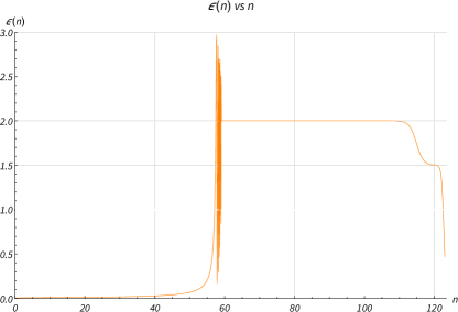
Figure 1: Evolution of the composite slow roll parameter (28) over cosmic history.

3.2 Dimensionless Formulation

It is desirable to convert the evolution variable from the co-moving time $t$ to the dimensionless number of e-foldings since the beginning of inflation, $n\equiv\ln[\frac{a(t)}{a(t_{i})}]$. The resulting change in calculus is,

$$\frac{d}{dt}=H\frac{d}{dn}\qquad,\qquad\frac{d^{2}}{dt^{2}}=H^{2}\Bigl{[}\frac{d^{2}}{dn^{2}}-\epsilon\frac{d}{dn}\Bigr{]}\qquad,\qquad\int\!\!dt=\int\!\!\frac{dn}{H}\;.$$ (29)

Hence the relation (13) between $\mathcal{T}[a](t)$ and $\mathcal{V}[a](t)$ becomes,

$$\mathcal{T}_{\rm ren}=-\frac{H^{2}}{2}\Bigl{[}\frac{d}{dn}+(3\!-\!\epsilon)\Bigr{]}\frac{d\mathcal{V}_{\rm ren}}{dn}\;.$$ (30)

And the key integral in expression (11) can be written as,

$$\int_{t_{i}}^{t}\!\!dt^{\prime}\frac{\mathcal{T}_{\rm ren}}{H(t^{\prime})}=-\frac{1}{2}\!\!\int_{0}^{n}\!\!dn^{\prime}\Bigl{[}\frac{d}{dn^{\prime}}+(3\!-\!\epsilon)\Bigr{]}\frac{d\mathcal{V}_{\rm ren}}{dn^{\prime}}\equiv-\frac{\mathcal{I}(n)}{16\pi G}\;.$$ (31)

3.3 Numerical Results

As Figure 2 shows, the running term (22) makes only a small contribution during inflation, and virtually nothing afterwards.

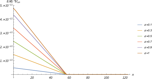
Figure 2: Evolution of ($8\pi G$ times) the running contribution (22) to the coincident propagator for different values of $\alpha$. Note that $\mathcal{V}_{\rm run}$ vanishes exactly during radiation domination, and is too small to show up afterwards.

Figure 3 shows the much larger contribution from the dimensionless integral $\mathcal{I}(n)$ which was defined in expression (31). Note that it grows during inflation, and then falls off afterwards. The expectation value of the dimensionless field can be expressed in terms of $\mathcal{I}(n)$ as,

$$\Bigl{\langle}\Omega\Bigl{|}\sqrt{8\pi G}\,A(x)\Bigr{|}\Omega\Bigr{\rangle}=\frac{2\sqrt{8\pi G}}{\lambda}\left[\sqrt{1\!+\!\frac{1}{12}\left(\frac{\lambda}{\sqrt{8\pi G}}\right)^{2}\mathcal{I}(n)}\!-\!1\right]+\Bigl{(}{\rm Stochastic\ acceleration}\Bigr{)}\;.$$ (32)

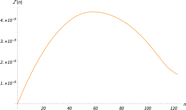
Figure 3: Evolution of $\mathcal{I}(n)$ from the beginning of primordial inflation to today.

Of course the right hand side of (32) depends on our choice of the dimensionless coupling constant $\lambda/\sqrt{8\pi G}$. Figure 4 shows the analytic part for a convenient choice. We have ignored the “stochastic acceleration” term which increases the growth during inflation, and disappears afterwards. Even at the present day one can see that the dimensionless field retains more than half the value it built up during inflation. Had we employed a model with a larger period of primordial inflation this effect would have been correspondingly greater.

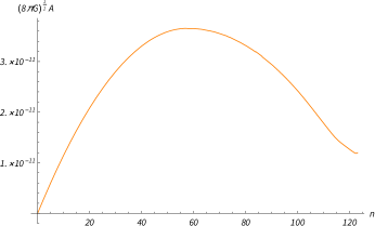
Figure 4: Evolution of the expectation value of $\sqrt{8\pi G}\,A$ for $\lambda=\frac{1}{10}\times\sqrt{8\pi G}$.

One can see from Figure 3 that $\mathcal{I}(n)$ is never larger than about $4\times 10^{-9}$. This is because the inflationary model of section 2 persists for only the minimum of 50-60 e-foldings required to explain the Horizon Problem. One can envisage much longer periods of inflation; extending the number of e-foldings by a factor increases the peak value of $\mathcal{I}(n)$ by roughly that same factor. Because the dimensionless coupling $\lambda/\sqrt{8\pi G}=\frac{1}{10}$ chosen for Figure 4 is of order one, the square root in equation (32) is near unity and perturbation theory never breaks down,

$${\rm Perturbative}\qquad\Longrightarrow\qquad\Bigl{\langle}\Omega\Bigl{|}\sqrt{8\pi G}\,A(x)\Bigr{|}\Omega\Bigr{\rangle}\simeq\frac{\lambda\mathcal{I}(n)}{12\sqrt{8\pi G}}\;.$$ (33)

However, expression (32) is nonpertutbative, and we can make perturbation theory break down, either by increasing the duration of primordial inflation or else by increasing the dimensionless coupling. The result in that case becomes,

$${\rm Nonperturbative}\qquad\Longrightarrow\qquad\Bigl{\langle}\Omega\Bigl{|}\sqrt{8\pi G}\,A(x)\Bigr{|}\Omega\Bigr{\rangle}\simeq\sqrt{\frac{\mathcal{I}(n)}{3}}\;.$$ (34)

Figure 5 illustrates this regime for $\lambda=10^{6}\times\sqrt{8\pi G}$.

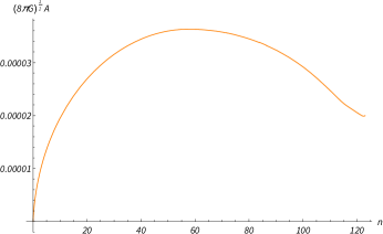
Figure 5: Evolution of the expectation value of $\sqrt{8\pi G}\,A$ for $\lambda=10^{6}\times\sqrt{8\pi G}$.

The alert reader will note from Figures 3 through 5 that the decrease due to modes experiencing 2nd horizon crossing ceases at the onset of the current phase of cosmic acceleration. Indeed, one might expect to see the decline reversed because modes again begin exiting the horizon. However, it must be recalled that the strength of the amplitude scales like the square of the Hubble parameter at 1st crossing, as per equation (62) in Ref. [32]. Because the current Hubble parameter is some 55 orders of magnitude smaller than its value during inflation, the predicted late time growth would not be visible on our plots, even if they were extended beyond the present time.

4 Conclusions

We have analyzed the evolution of the expectation value of the scalar field $A$ in a non-linear sigma model (4) on a general cosmological background (1) that experiences primordial inflation. We did this by solving the Starobinsky Langevin equation (7) for this theory [26] which involves $\mathcal{T}[a](t)$, the trace of the doubly differentiated, coincident propagator (10). Expression (13) gives $\mathcal{T}[a](t)$ in terms of the coincident propagator $\mathcal{V}[a](t)$. A good analytic approximation [32] for the dimensionally regulated, primitive form of $\mathcal{V}[a](t)$ was reviewed in section 2.1, and subjected to composite operator renormalization in section 2.2. The final result takes the form of a small “running” term proportional to the local Ricci scalar, plus a much larger contribution (23), with (16) and (17) pertaining during inflation and (18) and (19) afterwards.

Although our analytic approximations should apply for any cosmology which which has experienced primordial inflation, we devised an plausible expansion history in section 3.1 to provide explicit numerical results. Figure 1 shows the first slow roll parameter of this cosmology, from which the Hubble parameter and the scale factor can be constructed by integration. The small running contribution (22) to $\mathcal{V}[a](t)$ is shown in Figure 2. Figure 3 gives the key integral (31) which determines the expectation value of the field shown in Figures 4 and 5.

A major goal of this study was to quantify the extent to which the high scales of primordial inflation are transmitted to late times. In this regard it is worth noting that the expectation value of $A$ would vanish if the Universe was eternally radiation dominated (that is, $\epsilon(t)=2$), or if it was flat. The fact that we get nonzero results, even during radiation domination, is due to the initial phase of primordial inflation. Note also from Figures 4 and 5 that, even at very late times, the field retains a substantial amount of the amplitude it built up during primordial inflation. Note finally that an arbitrarily large amplitude could be built up by extending the duration of primordial inflation, whereas there can be no extension of the post-inflationary diminution.

This study demonstrates that it is not only possible to sum the series of leading logarithms of nonlinear sigma models on de Sitter, but also on an arbitrary cosmological background (1) which has undergone primordial inflation. And we have seen two crucial things:

• That evolution never stops; and

• That an arbitrarily large effect from primordial inflation can be transmitted to late times.

The next step is extending this formalism to quantum gravity in order to discover what becomes of graviton loop corrections such as (2-3) at late times and after perturbation theory has broken down.

Acknowledgements

This work was partially supported by NSF grant PHY-2207514 and by the Institute for Fundamental Theory at the University of Florida.

References

- [1] R. P. Woodard, Int. J. Mod. Phys. D 23, no.09, 1430020 (2014) doi:10.1142/S0218271814300201 [arXiv:1407.4748 [gr-qc]].
- [2] A. A. Starobinsky, JETP Lett. 30, 682-685 (1979)
- [3] V. F. Mukhanov and G. V. Chibisov, JETP Lett. 33, 532-535 (1981)
- [4] N. C. Tsamis and R. P. Woodard, Phys. Rev. D 54, 2621-2639 (1996) doi:10.1103/PhysRevD.54.2621 [arXiv:hep-ph/9602317 [hep-ph]].
- [5] S. P. Miao and R. P. Woodard, Class. Quant. Grav. 23, 1721-1762 (2006) doi:10.1088/0264-9381/23/5/016 [arXiv:gr-qc/0511140 [gr-qc]].
- [6] E. O. Kahya and R. P. Woodard, Phys. Rev. D 76, 124005 (2007) doi:10.1103/PhysRevD.76.124005 [arXiv:0709.0536 [gr-qc]].
- [7] K. E. Leonard and R. P. Woodard, Class. Quant. Grav. 31, 015010 (2014) doi:10.1088/0264-9381/31/1/015010 [arXiv:1304.7265 [gr-qc]].
- [8] J. Garriga and T. Tanaka, Phys. Rev. D 77, 024021 (2008) doi:10.1103/PhysRevD.77.024021 [arXiv:0706.0295 [hep-th]].
- [9] N. C. Tsamis and R. P. Woodard, Phys. Rev. D 78, 028501 (2008) doi:10.1103/PhysRevD.78.028501 [arXiv:0708.2004 [hep-th]].
- [10] J. F. Donoghue, Phys. Rev. D 50, 3874-3888 (1994) doi:10.1103/PhysRevD.50.3874 [arXiv:gr-qc/9405057 [gr-qc]].
- [11] J. F. Donoghue, [arXiv:gr-qc/9512024 [gr-qc]].
- [12] C. P. Burgess, Living Rev. Rel. 7, 5-56 (2004) doi:10.12942/lrr-2004-5 [arXiv:gr-qc/0311082 [gr-qc]].
- [13] J. F. Donoghue, AIP Conf. Proc. 1483, no.1, 73-94 (2012) doi:10.1063/1.4756964 [arXiv:1209.3511 [gr-qc]].
- [14] J. F. Donoghue, [arXiv:2211.09902 [hep-th]].
- [15] L. Tan, N. C. Tsamis and R. P. Woodard, Phil. Trans. Roy. Soc. Lond. A 380, 0187 (2021) doi:10.1098/rsta.2021.0187 [arXiv:2107.13905 [gr-qc]].
- [16] L. Tan, N. C. Tsamis and R. P. Woodard, Universe 8, no.7, 376 (2022) doi:10.3390/universe8070376 [arXiv:2206.11467 [gr-qc]].
- [17] S. P. Miao and R. P. Woodard, Phys. Rev. D 74, 024021 (2006) doi:10.1103/PhysRevD.74.024021 [arXiv:gr-qc/0603135 [gr-qc]].
- [18] S. P. Miao, Phys. Rev. D 86, 104051 (2012) doi:10.1103/PhysRevD.86.104051 [arXiv:1207.5241 [gr-qc]].
- [19] D. Glavan, S. P. Miao, T. Prokopec and R. P. Woodard, JHEP 03, 088 (2022) doi:10.1007/JHEP03(2022)088 [arXiv:2112.00959 [gr-qc]].
- [20] D. Glavan, S. P. Miao, T. Prokopec and R. P. Woodard, Class. Quant. Grav. 31, 175002 (2014) doi:10.1088/0264-9381/31/17/175002 [arXiv:1308.3453 [gr-qc]].
- [21] C. L. Wang and R. P. Woodard, Phys. Rev. D 91, no.12, 124054 (2015) doi:10.1103/PhysRevD.91.124054 [arXiv:1408.1448 [gr-qc]].
- [22] N. C. Tsamis and R. P. Woodard, Nucl. Phys. B 724, 295-328 (2005) doi:10.1016/j.nuclphysb.2005.06.031 [arXiv:gr-qc/0505115 [gr-qc]].
- [23] H. Kitamoto and Y. Kitazawa, Phys. Rev. D 83, 104043 (2011) doi:10.1103/PhysRevD.83.104043 [arXiv:1012.5930 [hep-th]].
- [24] H. Kitamoto and Y. Kitazawa, Phys. Rev. D 85, 044062 (2012) doi:10.1103/PhysRevD.85.044062 [arXiv:1109.4892 [hep-th]].
- [25] H. Kitamoto, Phys. Rev. D 100, no.2, 025020 (2019) doi:10.1103/PhysRevD.100.025020 [arXiv:1811.01830 [hep-th]].
- [26] S. P. Miao, N. C. Tsamis and R. P. Woodard, JHEP 03, 069 (2022) doi:10.1007/JHEP03(2022)069 [arXiv:2110.08715 [gr-qc]].
- [27] R. P. Woodard and B. Yesilyurt, [arXiv:2302.11528 [gr-qc]].
- [28] A. A. Starobinsky, Lect. Notes Phys. 246, 107-126 (1986) doi:10.1007/3-540-16452-9_6
- [29] A. A. Starobinsky and J. Yokoyama, Phys. Rev. D 50, 6357-6368 (1994) doi:10.1103/PhysRevD.50.6357 [arXiv:astro-ph/9407016 [astro-ph]].
- [30] V. K. Onemli and R. P. Woodard, Class. Quant. Grav. 19, 4607 (2002) doi:10.1088/0264-9381/19/17/311 [arXiv:gr-qc/0204065 [gr-qc]].
- [31] V. K. Onemli and R. P. Woodard, Phys. Rev. D 70, 107301 (2004) doi:10.1103/PhysRevD.70.107301 [arXiv:gr-qc/0406098 [gr-qc]].
- [32] E. Kasdagli, M. Ulloa and R. P. Woodard, [arXiv:2302.04808 [gr-qc]].
- [33] D. Glavan, T. Prokopec and V. Prymidis, Phys. Rev. D 89, no.2, 024024 (2014) doi:10.1103/PhysRevD.89.024024 [arXiv:1308.5954 [gr-qc]].
- [34] D. Glavan, T. Prokopec and D. C. van der Woude, Phys. Rev. D 91, no.2, 024014 (2015) doi:10.1103/PhysRevD.91.024014 [arXiv:1408.4705 [gr-qc]].
- [35] D. Glavan, T. Prokopec and T. Takahashi, Phys. Rev. D 94, 084053 (2016) doi:10.1103/PhysRevD.94.084053 [arXiv:1512.05329 [gr-qc]].
- [36] D. Glavan, T. Prokopec and A. A. Starobinsky, Eur. Phys. J. C 78, no.5, 371 (2018) doi:10.1140/epjc/s10052-018-5862-5 [arXiv:1710.07824 [astro-ph.CO]].
- [37] E. Belgacem and T. Prokopec, Phys. Lett. B 831, 137174 (2022) doi:10.1016/j.physletb.2022.137174 [arXiv:2111.04803 [astro-ph.CO]].
- [38] C. J. G. Vedder, E. Belgacem, N. E. Chisari and T. Prokopec, JCAP 03, 016 (2023) doi:10.1088/1475-7516/2023/03/016 [arXiv:2209.00440 [astro-ph.CO]].
- [39] A. Dolgov and D. N. Pelliccia, Nucl. Phys. B 734, 208-219 (2006) doi:10.1016/j.nuclphysb.2005.12.002 [arXiv:hep-th/0502197 [hep-th]].
- [40] C. Itzykson and J. B. Zuber, McGraw-Hill, 1980, ISBN 978-0-486-44568-7
- [41] S. Weinberg, Cambridge University Press, 2013, ISBN 978-1-139-63247-8, 978-0-521-67054-8, 978-0-521-55002-4 doi:10.1017/CBO9781139644174
- [42] Y. Akrami et al. [Planck], Astron. Astrophys. 641, A10 (2020) doi:10.1051/0004-6361/201833887 [arXiv:1807.06211 [astro-ph.CO]].
- [43] P. A. R. Ade et al. [BICEP and Keck], Phys. Rev. Lett. 127, no.15, 151301 (2021) doi:10.1103/PhysRevLett.127.151301 [arXiv:2110.00483 [astro-ph.CO]].
- [44] A. A. Starobinsky, Phys. Lett. B 91, 99-102 (1980) doi:10.1016/0370-2693(80)90670-X
- [45] N. Aghanim et al. [Planck], Astron. Astrophys. 641, A6 (2020) [erratum: Astron. Astrophys. 652, C4 (2021)] doi:10.1051/0004-6361/201833910 [arXiv:1807.06209 [astro-ph.CO]].