BayesCPclust: A Bayesian Approach for Clustering Constant-Wise Change-Point Data

Abstract

Change-point models deal with ordered data sequences. Their primary goal is to infer the locations where an aspect of the data sequence changes. In this paper, we propose and implement a nonparametric Bayesian model for clustering observations based on their constant-wise change-point profiles via Gibbs sampler. Our model incorporates a Dirichlet Process on the constant-wise change-point structures to cluster observations while simultaneously performing multiple change-point estimation. Additionally, our approach controls the number of clusters in the model, not requiring the specification of the number of clusters a priori. Satisfactory clustering and estimation results were obtained when evaluating our method under various simulated scenarios and on a real dataset from single-cell genomic sequencing. Our proposed methodology is implemented as an R package called BayesCPclust and is available at https://github.com/acarolcruz/BayesCPclust.

Keywords: Change-point models, Model-based clustering, Bayesian Inference, Dirichlet Process

1 Introduction

Change-point models deal with the analysis of an ordered sequence of random quantities. Examples of such sequences include daily average temperatures over time and sequencing data in genomics. An important component of a change-point model is change-point detection, which involves inferring the positions where an aspect of the data sequence changes, such as location or distribution. These change points and their corresponding locations are of great practical interest. One of the first applications of these models dates back to the 1950s when Page, (1954, 1955) introduced a now well-know sequential method called cumulative sum (CUSUM) to detect changes in the mean of a quality control process. Since then, change-point detection has been actively addressed in various application settings, such as financial analysis (Fryzlewicz,, 2014) and biostatistics (Olshen et al.,, 2004; Picard et al.,, 2011; Hocking et al.,, 2013). Change-point detection is also widely studied in time-series analysis (Jandhyala et al.,, 2013; Aue and Horváth,, 2013; Yan et al.,, 2019; Zhao et al.,, 2019; Militino et al.,, 2020); however, in what follows, we focus on non-time-series techniques.

Change-point models are generally divided into two main groups: online methods, which perform sequential detection with new data continually arriving, commonly used in anomaly detection, and offline methods, in which retrospective analysis is performed in the entire observed sequence (Truong et al.,, 2020). In this article, we focus on the latter. Additionally, change-point models may be either parametric or nonparametric. Parametric models assume that the underlying distributions belong to some known family. In contrast, nonparametric approaches heavily rely on the estimation of density functions, but may be employed in a broader range of applications (Brodsky and Darkhovsky,, 1993; Chen and Gupta,, 2012; Haynes et al.,, 2017; Londschien et al.,, 2023).

The literature on change-point models is vast, and several methods to perform change-point detection have been proposed in the past few decades, so we discuss here some approaches proposed for single and multiple change-point problems. For example, Olshen et al., (2004) and Fryzlewicz, (2014) proposed circular binary segmentation and wild binary segmentation, respectively, both based on the binary segmentation algorithm proposed by Vostrikova, (1981). These methods perform change-point tests sequentially to locate change points in the data sequence. Other methods, mainly used for multiple change-point problems, treat change-point detection as a model-selection problem and estimate change points via minimizing a criterion. These methods often require dynamic programming such as the pruned exactly linear time (PELT) algorithm (Killick et al.,, 2012) and the functional pruned (FP) algorithm (Rigaill,, 2015). Some well-known approaches for multiple change-point detection include the simultaneous multiscale change-point estimator (SMUCE) (Frick et al.,, 2014) and the heterogeneous simultaneous multiscale change-point estimator (H-SMUCE) (Pein et al.,, 2017), both based on a multiscale hypothesis testing, where the optimization process relies on the penalization of a test statistic. Additional approaches for change-point problems are described in Zou et al., (2014) and Niu et al., (2016).

While all previously described approaches have been proposed to detect change points from a unique sequence of data points, there needs to be more literature on clustering change-point data from multiple sequences, especially considering only model-based techniques. To our knowledge, techniques involving change-point estimation and model-based clustering have only been studied by Dass et al., (2015), Zhu and Melnykov, (2022), and Sarkar and Zhu, (2022). Zhu and Melnykov, (2022) proposed a finite Gaussian mixture model for clustering observations with a single change point, whereas Sarkar and Zhu, (2022) proposed a finite Negative Binomial mixture model for clustering multiple change-point data. Both approaches consider the Expectation and Maximization (EM) algorithm for estimating the cluster assignments and the model parameters. The single change-point detection in Zhu and Melnykov, (2022) is performed using exhaustively searches for changes in the mean or variance where competing models are compared based on the Bayesian information criterion (BIC). The multiple change-point approach detects changes in the mean of a count process by employing a combination of segmentation and an exhaustive search approach. Similar to the single change-point approach, the best model is selected based on the BIC. In Dass et al., (2015), focusing on the analysis of the mortality rate over time for 49 states in the United States, the authors Dass et al., (2015) took a Bayesian approach for clustering multiple change-point data by assuming a Functional Dirichlet Process on the linear piece-wise structure of their data to cluster states based on the change-point locations and slope magnitudes. The estimation of the model parameters and cluster assignments is performed via Gibbs sampler. Although these papers showed promising results in dealing with the problem of clustering change-point data while simultaneously performing change-point detection, none made their algorithm’s implementation available.

Bayesian techniques for change-point detection are known to provide state-of-the-art results in various settings, as stated in Dass et al., (2015); Truong et al., (2020). We propose and implement a nonparametric Bayesian model for clustering multiple constant-wise change-point data via Gibbs sampler. Similarly to Dass et al., (2015), our model incorporates a Functional Dirichlet Process on the constant-wise change-point structures that automatically controls the number of clusters in the model as opposed to other clustering techniques (Neal,, 1992; Yerebakan et al.,, 2014). To the best of our knowledge, this is the first paper to provide an implementation for the problem of clustering multiple change-point data while simultaneously performing change-point detection. We apply our proposed approach to cluster abnormal (tumour) single-cell genomic data based on their copy-number profiles, which resemble constant-wise structures. In addition, we evaluate the performance of our method under various simulated scenarios. Our proposed method is implemented as an R package called BayesCPclust and is available at https://github.com/acarolcruz/BayesCPclust.

The rest of the paper is organized as follows. Section 2 introduces our proposed methodology and provides the updating steps for the Gibbs sampler. Section 3 presents the performance results for our proposed method under various simulated scenarios. Finally, in Section 4, we show the application results of our method in a single-cell copy-number dataset.

2 Methods

Our proposed methodology extends the work of Dass et al., (2015) to cluster multiple constant-wise change-point data. Dass et al., analyzed the linear piece-wise structures of the mortality rate for 49 states in the United States. States were clustered based on the location and slope magnitudes of the change points by assuming a functional Dirichlet Process on the linear piece-wise data structure. In comparison, our method takes that a constant piece-wise form represents the data. Consequently, all derivations had to be recalculated. In what follows, we describe our model and in Section 2.1 we present the proposed Bayesian inference technique.

Let $\mathbf{Y}_{n}=(Y_{n1},\dotsc,Y_{nM})$ be a data sequence ordered based on some covariate such as time or position along a chromosome. For example, in the copy-number dataset in Section 4, $Y_{nm}$ represents the $\log 2$ ratio GC-corrected copy number aligned to genomic bin $m$ and cell $n$, where $n=1,\dotsc,N$, and $m=1,\dotsc,M$.

If we assume that there are $K_{n}$ change points in $\mathbf{Y}_{n}$, that means that $\mathbf{Y}_{n}$ can be partitioned into $K_{n}+1$ distinct segments, $[1,\tau^{(n)}_{1}),[\tau^{(n)}_{1},\tau^{(n)}_{2}),\dotsc,[\tau^{(n)}_{K_{n}},M]$, with change-point positions $\tau^{(n)}_{1},\dotsc,\tau^{(n)}_{K_{n}}$, such that $\tau^{(n)}_{0}=1$ and $\tau^{(n)}_{{K_{n}}+1}=M$. Also we assume that the change points are ordered, that is, $\tau^{(n)}_{i}<\tau^{(n)}_{j}$ if, and only if, $i<j$.

In our approach we assume a constant-wise structure for $Y_{nm}$ defined by the following the model:

$$Y_{nm}=\alpha_{l}^{(n)}+\epsilon_{nm},$$ (1)

where $m\in[\tau_{l-1}^{(n)},\tau_{l}^{(n)})$ for $l=1,\dotsc,K_{n}+1$ and $\epsilon_{nm}\sim N(0,\sigma_{n}^{2})$.

The model in Equation (1) assumes that the mean trend in each interval between change points is constant-wise, defined by an intercept $\alpha_{l}$, $l=1,...,K_{n}+1$, and an error term. Furthermore, this model allows the variability around the mean trend to differ depending on the observation by specifying a variance component $\sigma_{n}^{2}$ for each $n$.

Clustering change-point data via a Functional Dirichlet Process is formulated by assuming that the constant-wise structures for the observations are independent draws from some distribution, $G$, which in turn follows a Dirichlet Process prior. We define the constant-wise function as:

$$\boldsymbol{\theta}_{n}(m)=\alpha_{l}^{(n)},\qquad\text{if}\quad\tau_{l-1}^{(n)}\leq m\leq\tau_{l}^{(n)}-1,$$

where $\alpha_{l}^{(n)}$ is the intercept in the segment $[\tau_{l-1}^{(n)},\tau_{l}^{(n)})$ for each observation $n$. This constant-wise function, $\boldsymbol{\theta}_{n}(m)$, contains all information about the number of change points, their locations and the intercepts for the corresponding segment. Furthermore, a Dirichlet Process on $\boldsymbol{\theta}_{n}$ leads to the hierarchical model:

$$Y_{nm}\mid\boldsymbol{\theta}_{n},\sigma^{2}_{n} \sim N(\alpha_{l}^{(n)},\sigma^{2}_{n}),$$

$$\boldsymbol{\theta}_{n}\mid G \sim G,$$

$$G \sim DP(\alpha_{0},G_{0}),$$

where $G_{0}$ is the baseline distribution, such that $E(G)=G_{0}$, and $\alpha_{0}$ is the precision parameter that determines how distant the distribution $G\sim DP(\alpha_{0},G_{0})$ is from $G_{0}$.

Integration over $G$ allows the predictive distribution of $\boldsymbol{\theta}_{n}$ to be written as (Blackwell and MacQueen,, 1973):

$$\boldsymbol{\theta}_{n}\mid\boldsymbol{\theta}_{-n}\sim\frac{1}{N-1+\alpha_{0}}\sum_{j\neq n}\delta(\boldsymbol{\theta}_{j})+\frac{\alpha_{0}}{N-1+\alpha_{0}}G_{0},$$ (2)

where $\delta(\boldsymbol{\theta}_{j})$ is a point mass distribution at $\boldsymbol{\theta}_{j}$, and $-n$ represents all the observations except for $n$. Note that, by the first term in Equation (2), there is a positive probability that draws from $G$ will take on the same value. It implies that for a long enough sequence of draws from $G$, the value of any draw will be repeated by another draw, indicating that $G$ is a discrete distribution. Therefore, a Dirichlet Process on the change-point structures allows the proposed approach to control the number of clusters in the model, not requiring pre-specification. More details about the Dirichlet Process can be found in Neal, (2000) and Li et al., (2019).

We define the distribution $G_{0}$ in the following hierarchical form to cluster observations according to their constant-wise change-point profiles.

• Distribution of the number of change points ($K$): We assume that each segment between change points has at least $w>0$ points to ensure non-zero length. Let $m_{l}$ be the interval length of the $l$-th segment after subtracting $w$. As a result, $K\leq k^{*}$, where

  $$k^{*}=\frac{M-1}{w}-1$$

  to unsure that $m_{0}=\sum_{l=1}^{K+1}m_{l}=M-1-(K+1)w>0$.

  Therefore, $K$ follows a truncated Poisson distribution given by:

  $$P(K=k)=\frac{e^{-\lambda}\lambda^{k}/k!}{\displaystyle\sum_{l=0}^{k^{*}}e^{-\lambda}\lambda^{l}/l!},\quad\text{for }k=1,\dotsc,k^{*}.$$

• Distribution of the interval lengths between change points: Given $K=k$, the distribution of the interval lengths is defined as:

  $$(m_{1},\dotsc,m_{k+1})\mid K=k\sim\mathrm{Multinomial}\left(m_{0},\frac{1}{k+1},\dotsc,\frac{1}{k+1}\right).$$

  The change points positions, $\tau_{l}$, are obtained recursively by assuming that $\tau_{0}=1$, and $\tau_{l}=m_{l}+\tau_{l-1}+w$ for $l=1,\dotsc,k$.

• Distribution of the constant level $\alpha_{l}$: Given $K=k$, $\alpha_{l}$ is generated from the probability density function $\pi_{0}$ on $\mathbb{R}$ independently, where $\pi_{0}(\alpha_{l})\propto 1$ for $\alpha_{l}\in\mathbb{R}$, and $l=1,\dotsc,k+1$.

• Finally, the constant-wise structure, $\boldsymbol{\theta}_{n}(m)$, is then defined also based on the random quantities generated accordingly to their distribution defined in (i) - (iii).

• The baseline distribution $G_{0}$ is defined based on the distributions given in (i) - (iii):

  $$G_{0}(d\boldsymbol{\theta}) =\underbrace{P(K=k)}_{(i)}\underbrace{\left(\frac{\Gamma(m_{0}+1)}{\prod_{i=1}^{k}\Gamma(m_{i}+1)}\left(\frac{1}{k+1}\right)^{m_{0}}\right)}_{(ii)}\underbrace{\prod_{l=1}^{k+1}\pi_{0}(\alpha_{l})d\alpha_{l}}_{(iii)},$$

  where $dx$ represents an infinitesimal change in $x$. Therefore, $\pi_{0}(\alpha_{l})d\alpha_{l}$ corresponds to the probability of observing the infinitesimal interval in the neighbourhood of $\alpha_{l}$.

  Because $\pi_{0}(\alpha_{l})\propto 1$ for $l=1,\dotsc,k+1$, then $G_{0}(d\boldsymbol{\theta})\propto P(K=k)\left(\frac{\Gamma(m_{0}+1)}{\prod_{i=1}^{k}\Gamma(m_{i}+1)}\left(\frac{1}{k+1}\right)^{m_{0}}\right)$.

Note that, as mentioned, the distribution on the constant-wise structures, $G$, is discrete. Therefore, observations in cluster $r,$ for $r=1,\dotsc,d$ are assumed to share the same constant-wise function $\boldsymbol{\theta}_{r}$. Parameter estimation for the model is achieved in a Bayesian framework via a Gibbs sampler.

2.1 Bayesian Inference

The observed data is denoted by $\boldsymbol{Y}=(\boldsymbol{Y}_{1},\dotsc,\boldsymbol{Y}_{N})^{T}$, where $\boldsymbol{Y}_{n}=(Y_{n1},\dotsc,Y_{nM})^{T}$ for all observations $n=1,\dotsc,N$. $\underrightarrow{\boldsymbol{\theta}}=(\boldsymbol{\theta}_{1},\dotsc,\boldsymbol{\theta}_{N})$ is the collection of all constant-wise functions across all $N$ observations. Let $\boldsymbol{K}=(K_{1},\dotsc,K_{N})$ be the number of change points. We define the set of all change-point positions as $\boldsymbol{\tau}=(\boldsymbol{\tau}^{(n)},n=1,\dotsc,N)$ with $\boldsymbol{\tau}^{(n)}=(\tau_{1}^{(n)},\dotsc,\tau_{K_{n}}^{(n)})$, and $\boldsymbol{\alpha}=(\boldsymbol{\alpha}^{(n)},n=1,\dotsc,N)$ as the set of all intercept parameters with $\boldsymbol{\alpha}^{(n)}=(\alpha_{1}^{(n)},\dotsc,\alpha_{K_{n}+1}^{(n)})^{T}$. Let $X_{0}^{(n)}$ be the $M\times K_{n}+1$ design matrix for $\boldsymbol{\alpha}^{(n)}$.

The prior distributions for the intercepts $\boldsymbol{\alpha}^{(n)}$ and Dirichlet Process hyperparameters, $\alpha_{0}$ and $\lambda$, are respectively $\pi_{0}$, $\pi_{1}$ and $\pi_{2}$ so that:

$$\pi_{1}(\alpha_{0})=\mathrm{gamma}(a_{\alpha_{0}},b_{\alpha_{0}}),$$

and

$$\pi_{2}(\lambda)=\mathrm{gamma}(a_{\lambda},b_{\lambda}).$$

The prior distribution for the intercepts, $\pi_{0}$, is improper to provide analytical simplifications in the calculations for their posterior conditional distributions.

The variance components, $\boldsymbol{\sigma}^{2}=(\sigma_{1}^{2},\dotsc,\sigma_{N}^{2})$, are given independent inverse-gamma priors, such that

$$\pi_{3}(\boldsymbol{\sigma}^{2})=\prod_{n=1}^{N}\mathrm{Inverse\;Gamma}(a_{\sigma^{2}},b_{\sigma^{2}}).$$

2.1.1 Gibbs sampler

In this section we present the updating steps for the estimation of the parameters $\boldsymbol{\theta}_{n},$ $\boldsymbol{\sigma}^{2},$ $(\boldsymbol{\alpha}^{(r)},K_{r},\boldsymbol{\tau}^{(r)}),$ $\lambda$ and $\alpha_{0}$ for $n=1,\dotsc,N$ and $r=1,\dotsc,d$, where $r$ denotes a individual cluster and $d$ the total number of clusters. Each step involves calculating the full conditional distributions (see Appendix for derivation details).

Step 1: Update $\boldsymbol{\theta}_{n}$

The following expression demonstrates the clustering capability of the Dirichlet Process prior on the constant-wise structures $\boldsymbol{\theta}_{n}$. The current value of $\boldsymbol{\theta}_{n}$ can be selected to be one of the existing $\boldsymbol{\theta}_{r}$ with positive probability $\sum_{j=1}^{d}q_{n,j}/({q_{n,0}+\sum_{j=1}^{d}q_{n,j}})$. In case in which observation $n$ does not belong to any existing clusters, a new $\boldsymbol{\theta}_{n}$ is generate from the posterior distribution $G^{*}(\boldsymbol{\theta}_{n})$ as shown in Equation (3).

The posterior of $\boldsymbol{\theta}_{n}$ conditional on $\boldsymbol{\theta}_{-n}=(\boldsymbol{\theta}_{1},\dotsc,\boldsymbol{\theta}_{n-1},\boldsymbol{\theta}_{n+1},\dotsc,\boldsymbol{\theta}_{N})$ is given by

$$P(\boldsymbol{\theta}_{n}\mid\boldsymbol{\theta}_{-n},\boldsymbol{Y})=\frac{q_{n,0}G^{*}(d\boldsymbol{\theta}_{n})+\sum_{j=1}^{d}q_{n,j}\delta_{\boldsymbol{\theta}_{(j)}}}{q_{n,0}+\sum_{j=1}^{d}q_{n,j}},$$ (3)

where

$$q_{n,0}=\int_{\boldsymbol{\Theta}}\ell(\boldsymbol{Y}_{n}\mid\boldsymbol{\theta}_{n})G_{0}(d\boldsymbol{\theta}_{n})\alpha_{0}/(\alpha_{0}+N-1)\ \text{and}\ q_{n,j}=\ell(\boldsymbol{Y}_{n}\mid\boldsymbol{\theta}_{n})N_{r}/(\alpha_{0}+N-1),$$

define the mixing weights when observation $n$ forms a new cluster and when observation $n$ belongs to an existing cluster, respectively. Additionally,

$$G^{*}(d\boldsymbol{\theta}_{n})=\frac{\ell(\boldsymbol{Y}_{n}\mid\boldsymbol{\theta}_{n})G_{0}(d\boldsymbol{\theta}_{n})}{\int_{\boldsymbol{\Theta}}\ell(\boldsymbol{Y}_{n}\mid\boldsymbol{\theta}_{n})G_{0}(d\boldsymbol{\theta}_{n})}$$

is the posterior of $\boldsymbol{\theta}_{n}$ given that a new cluster is formed by observation $n$. Since $Y_{nm}\sim N(\alpha_{l}^{(n)},\sigma^{2}_{n})$, we have that $\ell(\boldsymbol{Y}_{n}\mid\boldsymbol{\theta}_{n})$ represents the normal likelihood function corresponding to the observation $\boldsymbol{Y}_{n}$ after integrating out the variance component $\sigma^{2}_{n}$. Also, $\alpha_{0}$ corresponds to the precision hyperparameter for the Dirichlet Process and $N_{r}$ denotes the number of observations in cluster $r$. The full expressions for $q_{n,0}$ and $q_{n,j}$ are given in detail in the Appendix Equations (7) and (8).

Step 2: Update $\sigma^{2}_{n}$

Regardless of whether $\boldsymbol{\theta}_{n}$ is a new value or an existing $\boldsymbol{\theta}_{r}$ (Step 1). The variance component for observation $n$ is updated using the full conditional of $\sigma^{2}_{n}$ given the other parameters.

$$P(\sigma^{2}_{n}\mid\boldsymbol{\theta}_{n},\boldsymbol{Y}_{n}) \propto f(\boldsymbol{Y}_{n}\mid\boldsymbol{\theta}_{n},\sigma_{n}^{2})\pi_{3}(\sigma^{2}_{n})$$

$$=\mathrm{Inverse\;Gamma}\left(\frac{N}{2}+a_{\sigma^{2}},\frac{(\boldsymbol{Y}_{n}-X_{0}\boldsymbol{\alpha}^{(n)})^{T}(\boldsymbol{Y}_{n}-X_{0}\boldsymbol{\alpha}^{(n)})}{2}+\frac{1}{b_{\sigma^{2}}}\right).$$

Step 3: Update $(K_{r},\boldsymbol{\tau}^{(r)},\boldsymbol{\alpha}^{(r)})$

$\underrightarrow{\boldsymbol{\theta}}$ uniquely determines the collection of parameters $(\boldsymbol{K},\boldsymbol{\tau},\boldsymbol{\alpha})$, and as mentioned, it contains several identical elements. Therefore, $(\boldsymbol{K},\boldsymbol{\tau},\boldsymbol{\alpha})$ also contains identical elements. In this step, we provide the updating procedures for the $d$ distinct components of $(\boldsymbol{K},\boldsymbol{\tau},\boldsymbol{\alpha})$, defined by $(K_{r},\boldsymbol{\tau}^{(r)},\boldsymbol{\alpha}^{(r)})$, for $r=1,\dotsc,d$, where $d$ is the number of clusters at the current update of the Gibbs sampler. Considering the hierarchical structure for the distributions of $\boldsymbol{\alpha}^{(r)}$ and $\boldsymbol{\tau}^{(r)}$, which both depends on the value of $K_{r}$, we first update $K_{r}$ from the posterior marginal probability function as follows:

$$P(K_{r}=k)\propto P(K=k)\sum_{(m_{1},\dotsc,m_{k+1})}v(m_{1},\dotsc,m_{k+1}),$$

where

$$v(m_{1},\dotsc,m_{k+1})=\exp{(\tilde{H}(m_{1},\dotsc,m_{k+1}))}\frac{\Gamma(m_{0}+1)}{\prod_{l=1}^{k+1}\Gamma(m_{l}+1)}\left(\frac{1}{k+1}\right)^{m_{0}}.$$

The full expression of $v(m_{1},\dotsc,m_{k+1})$ is given in detail in the Appendix Equations (9) and (5.1).

Then, we update $\boldsymbol{\tau}^{(r)}$ given $K_{r}=k$ using the probabilities $P(m_{1},\dotsc,m_{k+1})$, where

$$P(m_{1},\dotsc,m_{k+1})\propto v(m_{1},\dotsc,m_{k+1}).$$

This is carried out by exhaustively listing all combinations and numerically computing the corresponding probabilities.

Finally, $\boldsymbol{\alpha}^{(r)}$ given $\boldsymbol{\tau}^{(r)}$ and $K_{r}=k$ is updated based on the full conditional distribution:

$$P(\boldsymbol{\alpha}^{(r)}\mid\boldsymbol{\tau}^{(r)},K_{r},\boldsymbol{Y}_{r}) \propto f(\boldsymbol{Y}_{r}\mid\boldsymbol{\alpha}^{(r)},\boldsymbol{\sigma}^{2})\pi(\boldsymbol{\alpha}^{(r)})$$

$$=\mathrm{Normal}\left(V^{-1}_{r}X_{0,r}^{T}\boldsymbol{Y}_{n},V^{-1}_{r}\sum_{n\in C_{r}}\sigma^{-2}_{n}\right),$$

where $\boldsymbol{Y}_{r}$ represents the observations in cluster $r$.

Step 4: Update $\lambda$

The update of $\lambda$ is given by the following full conditional distribution and it is carried out by the Metropolis-Hasting algorithm; that is, we generate proposals from a gamma distribution and accept them with some probability based on an acceptance ratio.

$$P(\lambda\mid K,\boldsymbol{Y}) \propto\pi(\lambda)\prod_{n=1}^{N}P(K_{n}=k)$$

$$=\frac{1}{b^{a}\Gamma(a)}\lambda^{a-1}\exp\left\{\frac{\lambda}{b}\right\}\times\prod_{n=1}^{N}\frac{\lambda^{k}/k!}{\sum_{l=0}^{k^{*}}\lambda^{l}/l!}$$

$$\propto\frac{\lambda^{a-1+\sum_{n=1}^{N}K_{n}}}{\left(\sum_{l=0}^{k^{*}}\lambda^{l}/l!\right)^{N}}\exp\left\{\frac{\lambda}{b}\right\},$$

where $a$ and $b$ are the prior hyperparameters previously defined as $a_{\lambda}$ and $b_{\lambda}$.

Step 5: Update $\alpha_{0}$

The update of $\alpha_{0}$ is carried out using the procedure described in Escobar and West, (1998).

• Sample $u\sim\mathrm{Beta}(\alpha_{0}^{t-1}+1,N)$

• Draw $\alpha_{0}$ from the mixture $\pi_{u}\times\mathrm{Gamma}(a+d,(1/b-\log(u))^{-1})+(1-\pi_{u})\times\mathrm{Gamma}(a+d-1,(1/b-\log(u))^{-1})$,

where $a$ and $b$ are the prior hyperparameters previously described as $a_{\alpha_{0}}$ and $b_{\alpha_{0}}$, and $d$ is the number of clusters at the current update of the Gibbs sampler and the probability membership is

$$\pi_{u}=\frac{a+d-1}{N(1/b-\log(u))}.$$

3 Simulations

We evaluate the performance of our method through three simulated scenarios. We varied one of the parameters for each simulated scenario while fixing the others, as shown in Table 1. We apply our method to the 96 randomly generated datasets based on the model in Equation (1) considering the initialization for the Gibbs sampler as described in Section 3.1. Then, considering the evaluation metrics described in Section 3.2, we assess our method’s performance and results are presented in the following Sections 3.3, 3.4, and 3.5.

Table 1: Scenario configurations. We varied one of the parameters for each simulated scenario (shown by the * symbol), keeping the others fixed. The fixed parameters are $N=25$, $M=50$, $d=2$, and $K=2$. The possible values for the number of data sequences ($N$) are $10,25,50$, and for the number of locations ($M$) are $50,100,200$. Additionally, while varying the number of data sequences, we considered one simulated scenario where variance components ($\sigma^{2}_{n},n=1,\dotsc,N$) were generated from an inverse-gamma with a mean equal to 0.05, and another with a mean equal to 0.5.

Scenario	$\sigma^{2}$ (average)	$N$	$M$
1	0.05	*	50
2	0.50	*	50
3	0.05	25	*

3.1 Gibbs sampler initialization and implementation

This section describes the initialization for the Gibbs sampler and some details about our algorithm’s implementation. For the simulation scenarios and real data analysis, the hyperparameters for the prior distribution of the variance components were specified as $a_{\sigma^{2}}=2$ and $b_{\sigma^{2}}=1000$. For the prior distributions of $\lambda$ and $\alpha_{0}$, the hyperparameters were $a_{\lambda}=a_{\alpha_{0}}=2$ and $b_{\lambda}=b_{\alpha_{0}}=1000$.

To enable convergence diagnosis for the Gibbs sampler we employed two chains with different initial values for each simulated scenario. The first chain starts from the true settings, that is, we consider the parameter values used to generate the datasets as initial values for our algorithm, whereas for the second chain we initialize the Gibbs sampler from the true parameter values plus a small perturbation. For instance, the initial values for the intercepts of each cluster are initialized from the true setting plus 1.5. The position of the change points for each cluster starts from two points above the ground truth and the variance components are initialized using generated values from an inverse-gamma distribution with twice the average used to generate the true variance components.

The simulations and computations for the Gibbs sampler algorithm were performed using Sharcnet’s Graham cluster, with a single node consisting of two Intel E5-2683 v4 “Broadwell” with 2.1GHz processor base frequency, for an overall of 32 computing cores. The number of simulated datasets, S = 96, was chosen as a multiple of the number of cores. The computations were performed on [CentOS 7], with R version [4.2.1 “Funny-Looking Kid”] (R Core Team,, 2022), using the parallel package (R Core Team,, 2022) to simulate and to compute the Gibbs sampler for independent datasets simultaneously, the extraDistr package (Wolodzko,, 2020) to generate samples from inverse-gamma distributions, the RcppAlgos package (Wood,, 2023) to generate all possible partitions for the number of points in each segment between two change points, the MASS package (Venables and Ripley,, 2002) to generate samples from multivariate normal distributions, and the package FDRSeg (Rosenberg and Hirschberg,, 2007) to calculate the V-measure. It is worth mentioning that our algorithm is implemented as an R package and is available at https://github.com/acarolcruz/BayesCPclust.

3.2 Performance metrics

For each chain, simulated setting, and randomly generated dataset, we employ our method with 5000 iterations to estimate change points and perform clustering. We consider a burn-in of $50\%$ of the size of the chains, and we thin our remaining samples by keeping only every 25th iteration. This procedure ensures that our samples are not highly correlated. For the 200 remaining samples, we calculate the posterior mean for each parameter, except for the discrete variables, such as cluster assignments, number of clusters, number of change points, and their locations, where we choose the most frequent value, the posterior mode.

To evaluate our method’s performance concerning intercept estimation, we compute the average of the posterior means for each intercept and compare its value to the true settings considered when generating the datasets. We report the posterior means standard error and the average interval length of $95\%$ equal-tailed credible intervals taken over the 96 datasets to measure the precision of our estimates. Additionally, we report the MAD (Mean Absolute Deviation) for the variance components estimates.

For the discrete variables, we report the proportion of datasets in which we correctly estimated the parameters. To evaluate the clustering performance of our proposed approach, we consider the V-measure (Rosenberg and Hirschberg,, 2007), which assesses observation-to-cluster assignments and measures the homogeneity and completeness of a clustering result. The V-measure ranges from zero to one, where results closer to one are considered adequate.

3.3 Scenario 1: Varying the number of data sequences with $\sigma_{n}^{2}\approx 0.05$

Figure 1 shows the data structure of four data sequences from one of the 96 randomly generated synthetic datasets for Scenario 1 when $N=50$. In this scenario, we vary the number of data sequences considering $N=10,25$, and $50$ while keeping the other parameters fixed as described in Table 1. Each panel represents one observation colored by their cluster assignment. Both clusters have two change points. Change-point locations for Cluster 1 are 19 and 34; for the second cluster, they are 15 and 32. Each segment between change points is defined by a constant level (5, 20, and 10) for the first cluster and (17, 10, and 2) for the second cluster.

Figure 1: Simulation scenario 1. Data structure for four data sequences from one of the 96 randomly generated synthetic datasets for Scenario 1 ($N=50\text{ and }M=50$) with $\sigma^{2}_{n}\approx 0.05$. Each panel presents the observed values for one data sequence. Observations from cluster 1 are colored in red, whereas observations from cluster 2 are colored in blue.

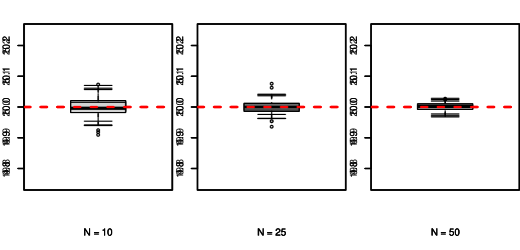
(a)

(b)

(c)

Figure 2: Simulation scenario 1, cluster 1. Boxplots of the posterior mean estimates for the intercepts (a) $\alpha_{1}$, (b) $\alpha_{2}$, and (c) $\alpha_{3}$ of our change-point model for cluster 1 based on the 96 randomly generated synthetic data sets, when we vary the number of observations $N$ with $\sigma^{2}_{n}\approx 0.05$. The red dashed lines correspond to the true parameter values for each intercept.

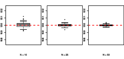
(a)

(b)

(c)

Figure 3: Simulation scenario 1, cluster 2. Boxplots of the posterior mean estimates for the intercepts (a) $\alpha_{1}$, (b) $\alpha_{2}$, and (c) $\alpha_{3}$ of our change-point model for cluster 2 based on the 96 randomly generated synthetic data sets, when we vary the number of observations $N$ with $\sigma^{2}_{n}\approx 0.05$ . The red dashed lines correspond to the true parameter values for each intercept.

Table 2: Simulation scenario 1. Posterior estimates for the intercepts of each cluster taken over 96 randomly generated synthetic datasets when we vary the number of observations ($N$). The variance components in this scenario were sampled from an inverse gamma with small average (0.05). We report the average posterior mean estimates (Average) and standard error (SE) for each intercept, and we present the average interval length of $95\%$ credible intervals (Average CI size) taken over the 96 datasets.

Cluster	Parameter	$N$	Average	SE	Average CI size
		10	4.9997	0.0260	0.0874
	$\alpha_{1}=5$	25	4.9997	0.0169	0.0597
		50	5.0001	0.0101	0.0389
		10	20.0027	0.0285	0.0943
1	$\alpha_{2}=20$	25	20.0009	0.0217	0.0665
		50	20.0010	0.0129	0.0425
		10	9.9977	0.0259	0.0897
	$\alpha_{3}=10$	25	10.0000	0.0144	0.0628
		50	10.0005	0.0118	0.0403
		10	17.0069	0.0279	0.1031
	$\alpha_{1}=17$	25	17.0027	0.0179	0.0658
		50	17.0002	0.0113	0.0432
		10	10.0005	0.0298	0.0940
2	$\alpha_{2}=10$	25	9.9991	0.0159	0.0596
		50	9.9988	0.0116	0.0387
		10	1.9994	0.0253	0.0876
	$\alpha_{3}=2$	25	2.0003	0.0150	0.0568
		50	2.0000	0.0095	0.0376

Based on the methodology of Gelman and Rubin, (1992), the convergence of the chains for all parameters, after the burn-in period and thinning procedure was confirmed. Table 2 and Figures 2 and 3 display the results for the posterior estimates for the intercepts of each cluster when the number of data sequences is $N=$ 10, 25, and 50, and the variance components were generated around 0.05. In this setting, our estimates were close to the true parameter values, showing that our proposed method retrieved the correct intercepts for each cluster. As the number of data sequences increases, the standard error of our intercept estimates and the average length of the $95\%$ credible intervals decreases, as expected. Considering that each data sequence has its own variance component and $M$ is fixed, increasing the number of data sequences does not considerably improve the estimation of the variance components as shown in Table 3 by the mean absolute deviation.

Table 3: Simulation scenario 1. Mean absolute deviation (MAD) for the estimated variances (as the posterior means) when we vary the number of data sequences and the variance components were sampled from an inverse-gamma with average 0.05.

$N$	MAD
10	0.0073
25	0.0091
50	0.0079

The change point locations associated with the two clusters were correctly estimated for all 96 datasets. The number of clusters, and the cluster assignment for each data sequence were correctly estimated for all 96 datasets resulting in all V-measures to be equal to one.

3.4 Scenario 2: Varying the number of data sequences with $\sigma_{n}^{2}\approx 0.50$

This section evaluates our method’s performance with a higher data dispersion than in the previous section. We generate 96 datasets as in the last experiment for each possible value of $N$; however, for this scenario, we sample the variance components from an inverse gamma with an average 10 times higher than in the simulation Scenario 1 as shown in Figure 4.

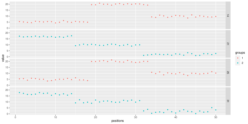
Figure 4: Simulation scenario 2. Data structure for four data sequences from one of the 96 randomly generated synthetic datasets for Scenario 2 ($N=50\text{ and }M=50$) with $\sigma^{2}_{n}\approx 0.5$. Each panel presents the observed values for one data sequence. Observations from cluster 1 are colored in red, whereas observations from cluster 2 are colored in blue.

It is worth mentioning that the convergence of the chains for all parameters in Scenario 2 was also confirmed using the methodology of Gelman and Rubin, (1992). Table 4 and Figures 5 and 6 show the results for the posterior estimates for the intercepts of each segment between change points for the two clusters when the number of data sequences is $N=10$, $25$ and $50$ and the variance components were generated around 0.5. We observe that for each possible value for the number of data sequences, our approach correctly estimated the intercepts. However, the standard errors of our estimates are noticeably higher than in the previous scenario due to the increase in the data dispersion. Nonetheless, our method showed good performance, not only in estimating the intercepts for each cluster but also in correctly estimating the number of change points and their corresponding locations. Additionally, our method always recovered the true clustering configuration in our data, with all V-measures equal to one.

Furthermore, the mean absolute deviation for the variance components estimates remained stable, as in the previous scenario, suggesting that increasing the number of data sequences does not noticeably improve the precision of the variance component estimates as reported in Table 5.

(a)

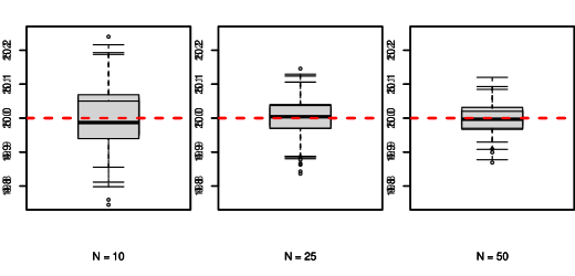
(b)

(c)

Figure 5: Simulation scenario 2, cluster 1. Boxplots of the posterior mean estimates for the intercepts (a) $\alpha_{1}$, (b) $\alpha_{2}$, and (c) $\alpha_{3}$ of our change-point model for cluster 1 based on the 96 randomly generated synthetic data sets, when we vary the number of observations $N$ with $\sigma^{2}_{n}\approx 0.5$. The red dashed lines correspond to the true parameter values for each intercept.

(a)

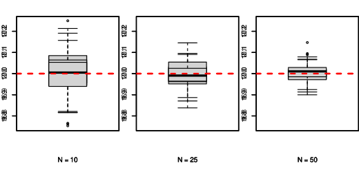
(b)

(c)

Figure 6: Simulation scenario 2, cluster 2. Boxplots of the posterior mean estimates for the intercepts (a) $\alpha_{1}$, (b) $\alpha_{2}$, and (c) $\alpha_{3}$ of our change-point model for cluster 2 based on the 96 randomly generated synthetic data sets, when we vary the number of observations $N$ with $\sigma^{2}_{n}\approx 0.5$ . The red dashed lines correspond to the true parameter values for each intercept.

Table 4: Simulation scenario 2. Posterior estimates for the intercepts of each cluster taken over 96 randomly generated synthetic datasets when we vary the number of observations ($N$). The variance components in this scenario were sampled from an inverse-gamma with average equals to 0.50. We report the average posterior mean estimates (Average) and standard error (SE) for each intercept, and we present the average interval length of $95\%$ credible intervals (Average CI size) taken over the 96 datasets.

Cluster	Parameter	$N$	Average	SE	Average CI size
		10	4.9990	0.0825	0.2773
	$\alpha_{1}=5$	25	5.0086	0.0508	0.1801
		50	5.0021	0.0352	0.1265
		10	20.0077	0.0906	0.3015
1	$\alpha_{2}=20$	25	19.9953	0.0558	0.1992
		50	19.9990	0.0481	0.1389
		10	9.9929	0.0831	0.2821
	$\alpha_{3}=10$	25	10.0056	0.0493	0.1849
		50	9.9956	0.0374	0.1315
		10	17.0218	0.0882	0.3246
	$\alpha_{1}=17$	25	16.9916	0.0526	0.2000
		50	16.9989	0.0399	0.1431
		10	10.0021	0.0938	0.2962
2	$\alpha_{2}=10$	25	10.0083	0.0586	0.1799
		50	9.9958	0.0363	0.1273
		10	1.9977	0.0804	0.2784
	$\alpha_{3}=2$	25	1.9946	0.0441	0.1737
		50	2.0045	0.0317	0.1204

Table 5: Simulation scenario 2. Mean absolute deviation (MAD) for the estimated variances (as the posterior means) when we vary the number of data sequences and the variance components were sampled from an inverse-gamma with average 0.5.

$N$	MAD
10	0.0736
25	0.0784
50	0.0833

3.5 Scenario 3: Varying the number of locations

In this Section, we present the performance results of our method when the number of locations is $M=$ 50, 100, and 200. Table 6 and Figures 7 and 8 present the results for the intercepts for each case in the Scenario 3. As in the previous scenarios, convergence of the chains for all parameters was confirmed. Based on the results, our approach correctly estimated the intercepts for each cluster and showed that as the number of locations increased, the precision of our estimates improved. Once again, our method correctly estimated the number of change points and change-point positions for all generated datasets. In addition, all V-measures were equal to one, showing that our model recovered the true clustering configuration in our data.

Furthermore, in this scenario, we observed an increase in the precision of our estimates for the variance components, as shown in Table 7 as $M$ increases. As discussed in the previous scenarios, the number of data sequences minimally affects the precision of our variance estimates since each data sequence has its variance component. However, by increasing the number of locations, we noted a decrease in the mean absolute deviation for our estimates, suggesting that the number of locations considerably affects the estimation of the variance components.

(a)

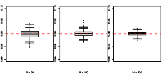
(b)

(c)

Figure 7: Simulation scenario 3, cluster 1. Boxplots of the posterior mean estimates for the intercepts (a) $\alpha_{1}$, (b) $\alpha_{2}$, and (c) $\alpha_{3}$ of our change-point model for cluster 2 based on the 96 randomly generated synthetic data sets, when we vary the number of locations $M$. The red dashed lines correspond to the true parameter values for each intercept.

(a)

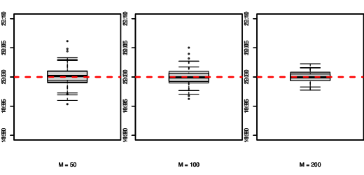
(b)

(c)

Figure 8: Simulation scenario 3, cluster 2. Boxplots of the posterior mean estimates for the intercepts (a) $\alpha_{1}$, (b) $\alpha_{2}$, and (c) $\alpha_{3}$ of our change-point model for cluster 2 based on the 96 randomly generated synthetic data sets, when we vary the number of locations $M$. The red dashed lines correspond to the true parameter values for each intercept.

Table 6: Simulation scenario 3. Posterior estimates for the intercepts of each cluster taken over 96 randomly generated synthetic datasets when we vary the number of locations ($M$). We report the average posterior mean estimates (Average) and standard error (SE) for each intercept, and we present the average interval length of $95\%$ credible intervals (Average CI size) taken over the 96 datasets.

Cluster	Parameter	$M$	Average	SE	Average CI size
		50	1.9999	0.0152	0.0574
	$\alpha_{1}=2$	100	2.0003	0.0099	0.0416
		200	2.0004	0.0085	0.0323
		50	14.9996	0.0165	0.0560
1	$\alpha_{2}=15$	100	15.0014	0.0103	0.0412
		200	15.0011	0.0083	0.0319
		50	6.9966	0.0157	0.0619
	$\alpha_{3}=7$	100	7.0013	0.0138	0.0480
		200	7.0012	0.0068	0.0271
		50	19.9997	0.0181	0.0615
	$\alpha_{1}=20$	100	19.9990	0.0126	0.0455
		200	20.0009	0.0100	0.0340
		50	5.0008	0.0147	0.0560
2	$\alpha_{2}=5$	100	5.0005	0.0119	0.0447
		200	4.9992	0.0067	0.0266
		50	12.0014	0.0122	0.0526
	$\alpha_{3}=12$	100	11.9990	0.0108	0.0368
		200	11.9995	0.0080	0.0341

Table 7: Simulation scenario 3. Mean absolute deviation (MAD) for the estimated variances (as the posterior means) when we vary the number of locations.

$M$	MAD
50	0.0076
100	0.0057
200	0.0041

4 Real data

We further assessed the performance of our method in a real dataset. We apply our approach to the copy number genomic data analyzed in Leung et al., (2017). The dataset consists of copy-number information for 45 cells (data sequences) from frozen primary tumors and liver metastases of colorectal cancer (CRC) patients. We chose to work with the data for patient CR2, which is more complex than patient CR1. Each data point in the dataset corresponds to the $\log_{2}$ ratio of reads aligned per 200-kb genomic bin per cell after GC correction. The $\log_{2}$ ratios provide an indication of the number of copies in each genomic bin. A $\log_{2}$ ratio greater than one means an amplification in the corresponding region.

In this paper, for computational purposes, we focus our analysis on chromosomes 19, 20, and 21, corresponding to 583 genomic bins (locations), since it is a region with visible change points. The raw data (FASTQ files) are available publicly at NCBI Sequence Read Archive (SRA) under accession number SRP074289. Processed $\log_{2}$ ratios were kindly provided by the authors of Leung et al., (2017) upon our request.

In the dataset, there are two main groups of cells, primary and metastatic tumour cells, that were labeled P and M, respectively. Figure 9 displays the copy-number data for six cells, three from each group. Primary tumour cells have copy-number log ratios close to two on chromosome 20 and around one in the remaining chromosomes. In contrast, the log-ratio reads are steady around one for all locations for metastatic tumour cells.

Figure 9: Copy-number data for chromosomes 19, 20 and 21 for six cells, three from primary tumour cells (P) and three from metastatic tumour cells (M). Due to computational cost, read positions were transformed using a Median Moving Window of size five, reducing the total number of genomic bins to 290.

Due to computational cost, we fixed the maximum number of change points ($k^{*}$) to two, and we applied a Median Moving Window of size five to each data sequence using the zoo package in R (Zeileis and Grothendieck,, 2005) to reduce the number of bins in the data and to handle possible outliers. Considering the transformed data, with 290 locations, we applied our algorithm using two chains of size 10 000; one was initialized using the clustering result from the K-means method when we set the number of clusters to be two. The other chain was initialized using random cluster assignments; that is, each cell was randomly assigned to one of two clusters. The number of change points for each cluster was set to zero at the beginning of the chains. Additionally, the initial values for the intercepts were selected as the average $\log_{2}$ ratio copy-number information taken over the cells in each initial cluster, and the sample variances were set as initial values for the variance components. The minimum number of locations in each segment between change points, $w$, was set to 50. Furthermore, convergence was confirmed using the methodology of Gelman and Rubin, (1992) for each chain after the burn-in of half the size of the chains and thinning the remaining samples by selecting every 50th.

Our approach identified three clusters: Cluster 1 is composed of only primary tumour cells with clear change points at bin locations 100 and 226, Cluster 2 with both primary and metastatic tumour cells with log-ratio reads around one for all bins, and Cluster 3 with only metastatic tumour cells with two change points at bin locations 165 and 215, as shown in Figures 10, 11 and 12.

Table 8 reports the posterior estimates for the intercepts of each segment between change points for each cluster, where we note that the intercepts for Cluster 2 are not significant since the credible intervals overlap, suggesting as is shown in Figure 11 the absence of change points since the log-ratio reads are steady around one for all locations. Interestingly, the cells belonging to Cluster 2 were not considered in the hierarchical clustering analysis in Leung et al., (2017). In addition, metastatic and primary tumour single cells were mainly clustered separately, as observed in Leung et al., (2017). However, Leung et al., considered all chromosomes when clustering cells and found two clusters for the metastatic tumour cells. Furthermore, they noted that amplifications of chromosomes 3 and 8 distinguished the subpopulations for the metastatic tumour cells. This data was also analyzed in Safinianaini et al., (2020), where the authors developed a Markov-Chain-based method for clustering copy number data. Analyzing the same data set, Safinianaini et al., considered the copy-number data for chromosomes 18 to 21 from patient CR2 to cluster tumour single-cells according to their copy-number profiles. As a result, Safinianaini et al., identified two clusters of tumour single-cells, separating primary from metastatic single-cells.

Figure 10: Copy-number data for all 18 cells in Cluster 1 composed of primary tumour cells. Our approach estimated two change points at positions 100 and 226. The black dashed lines correspond to the mean constant level for each segment between change points.

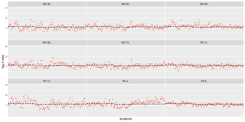
Figure 11: Copy-number data for all nine cells in Cluster 2 composed of tumour cells with copy-number reads around one in all locations. The black dashed lines correspond to the mean constant level for each segment between change points.

Figure 12: Copy-number data for all 18 cells in Cluster 3 composed of metastatic tumour cells with change points at positions 165 and 215. The black dashed lines correspond to the mean constant level for each segment between change points.

Table 8: Posterior estimates for the intercepts of each identified cluster. We report the average posterior mean estimates (Average) and standard error (SE) for each intercept, and the $95\%$ credible interval ($95\%$ CI).

Cluster	Parameter	Average	SE	95% CI
	$\alpha_{1}$	1.2536	0.0051	[1.2435, 1.2638]
1	$\alpha_{2}$	1.9158	0.0044	[1.9070, 1.9250]
	$\alpha_{3}$	1.0063	0.0061	[0.9930, 1.0170]
	$\alpha_{1}$	1.1588	0.0127	[1.1322, 1.1757]
2	$\alpha_{2}$	1.0702	0.0721	[1.0161, 1.2301]
	$\alpha_{3}$	1.1048	0.0180	[1.0655, 1.1235]
	$\alpha_{1}$	1.2496	0.0043	[1.2417, 1.2568]
3	$\alpha_{2}$	1.5595	0.0270	[1.5295, 1.6186]
	$\alpha_{3}$	1.0732	0.0082	[1.0596, 1.0877]

5 Conclusion

The results from the simulation scenarios show that our approach can recover the true classification of each data sequence. Furthermore, it is precise in identifying the change points when we vary the number of data sequences and the number of locations. Additionally, the dispersion degree in our data did not affect the performance of our model, where we observed satisfactory results for both scenarios in which we sampled the variance components from inverse-gamma distributions with small and large averages. Finally, by applying our method to a copy-number single-cell dataset, our approach showed consistent results with the original paper Leung et al., (2017), where we obtained similar clusters for tumour single-cells based on their change-point structures.

The limitation of our approach lies in the computational cost since it requires the calculation of a probability for each possible combination of interval length between change points, which can be computationally expensive when the number of locations increases. To remedy this, in the real data analysis, we calculated the probabilities for a sample of all possible combinations of interval lengths, reducing but not sufficiently the computational cost. In general, as the number of data sequences or locations increases, the average processing time to infer change points and perform clustering analysis for the simulation scenarios also increases, where the highest processing time, 256 minutes (see Table 11 in the Appendix), was observed in the setting in which we considered 200 locations for each data sequence. Furthermore, we observed similar processing times for the first two scenarios (see Tables 9 and 10 in the Appendix), suggesting that the data dispersion had a minimal effect on the computational cost of our algorithm.

A common issue in Bayesian mixture modeling is that the labels of the clusters can be permuted multiple times over iterations of a Markov Chain Monte Carlo (MCMC) method, such as the Gibbs sampler. This issue, known as label switching, happens since the data likelihood is invariant under the permutation of the labels of the clusters. Solutions for undoing label switching are necessary to perform cluster-specific inference. Thus, various approaches have been proposed to solve this issue (Jasra et al.,, 2005; Papastamoulis and Iliopoulos,, 2010; Rodriguez and Walker,, 2014). In this paper, we assigned the most frequent set of labels to the sequences of cluster assignments leading to the same clustering. Then, after this correction for label switching, we obtained all the corresponding parameter posterior estimates for each cluster.

As a possible future work, other Bayesian Inference approaches for optimization can be considered, such as Variational Inference and Approximate Bayesian computation methods (Blei et al.,, 2017; van de Schoot et al.,, 2021), that produce functional approximations of the posterior distributions, which can reduce the computational cost of MCMC-based methods. Also, the Gibbs sampler developed in this paper can be improved using blocking, collapsing, and partial collapsing techniques for improving slow convergence in Gibbs sampler (Park and Lee,, 2022).

Appendix

5.1 Gibbs sampler

Step 1.

In this step we update the clustering assignments for the observations which depends on

$$q_{n,0}=\alpha_{0}\sum_{k=0}^{k^{*}}\sum_{(m_{1},\dotsc,m_{k+1})}H(m_{1},\dotsc,m_{k+1})\frac{m_{0}}{m_{1}!\dotsm m_{k+1}!}\left(\frac{1}{k+1}\right)^{m_{0}}P(K=k),$$

where

$$H(m_{1},\dotsc,m_{k+1}) =\int_{\boldsymbol{\alpha}^{(n)}}\int_{0}^{\infty}f(\boldsymbol{Y}_{n}\mid\boldsymbol{\alpha}^{(n)},\sigma^{2}_{n})\pi_{3}(\sigma^{2}_{n})d\sigma^{2}_{n}d\boldsymbol{\alpha}^{(n)}$$

$$=\int_{0}^{\infty}\int_{\boldsymbol{\alpha}^{(n)}}f(\boldsymbol{Y}_{n}\mid\boldsymbol{\alpha}^{(n)},\sigma^{2}_{n})\pi_{3}(\sigma^{2}_{n})d\boldsymbol{\alpha}^{(n)}d\sigma^{2}_{n},$$

with

$$f(\boldsymbol{Y}_{n}\mid\boldsymbol{\alpha}^{(n)},\sigma^{2}_{n})=\frac{1}{(2\pi\sigma^{2}_{n})^{N/2}}\exp\left\{-\frac{1}{2\sigma^{2}_{n}}(\boldsymbol{Y}_{n}-X_{0}\boldsymbol{\alpha}^{(n)})^{T}(\boldsymbol{Y}_{n}-X_{0}\boldsymbol{\alpha}^{(n)})\right\}$$

and

$$\int_{{\boldsymbol{\alpha}}^{(n)}}f(\boldsymbol{Y}_{n}\mid\boldsymbol{\alpha}^{(n)},\sigma^{2}_{n})d\boldsymbol{\alpha}^{(n)}=\int_{{\boldsymbol{\alpha}}^{(n)}}\frac{1}{(2\pi\sigma^{2}_{n})^{N/2}}\exp\left\{-\frac{1}{2\sigma^{2}_{n}}(\boldsymbol{Y}_{n}-X_{0}\boldsymbol{\alpha}^{(n)})^{T}(\boldsymbol{Y}_{n}-X_{0}\boldsymbol{\alpha}^{(n)})\right\}d\boldsymbol{\alpha}^{(n)}.$$ (4)

We calculate $(\boldsymbol{Y}_{n}-X_{0}\boldsymbol{\alpha}^{(n)})^{T}(\boldsymbol{Y}_{n}-X_{0}\boldsymbol{\alpha}^{(n)})$ in (4) as:

$$(\boldsymbol{Y}_{n}-X_{0}\boldsymbol{\alpha}^{(n)})^{T}(\boldsymbol{Y}_{n}-X_{0}\boldsymbol{\alpha}^{(n)}) =\boldsymbol{Y}^{T}_{n}\boldsymbol{Y}_{n}-\boldsymbol{\alpha}^{T(n)}X_{0}^{T}\boldsymbol{Y}_{n}-\boldsymbol{Y}^{T}_{n}X_{0}\boldsymbol{\alpha}^{(n)}+\boldsymbol{\alpha}^{T(n)}X_{0}^{T}X_{0}\boldsymbol{\alpha}^{(n)}$$

$$=\boldsymbol{Y}^{T}_{n}\boldsymbol{Y}_{n}-2\boldsymbol{Y}^{T}_{n}X_{0}\boldsymbol{\alpha}^{(n)}+\boldsymbol{\alpha}^{T(n)}X_{0}^{T}X_{0}\boldsymbol{\alpha}^{(n)},$$ (5)

where we can complete the square as follows:

$$(\boldsymbol{\alpha}^{(n)}-(X_{0}^{T}X_{0})^{-1}X_{0}^{T}\boldsymbol{Y}_{n})^{T}(X_{0}^{T}X_{0})(\boldsymbol{\alpha}^{(n)}-(X_{0}^{T}X_{0})^{-1}X_{0}^{T}\boldsymbol{Y}_{n})$$

$$=(\boldsymbol{\alpha}^{T(n)}-\boldsymbol{Y}^{T}_{n}X_{0}(X_{0}^{T}X_{0})^{-1})(X_{0}^{T}X_{0}\boldsymbol{\alpha}^{(n)}-X_{0}^{T}X_{0}(X_{0}^{T}X_{0})^{-1}X_{0}^{T}\boldsymbol{Y}_{n})$$

$$=\boldsymbol{\alpha}^{T(n)}X_{0}^{T}X_{0}\boldsymbol{\alpha}^{(n)}-\boldsymbol{\alpha}^{T(n)}X_{0}^{T}\boldsymbol{Y}_{n}-\boldsymbol{Y}^{T}_{n}X_{0}\boldsymbol{\alpha}^{(n)}+\boldsymbol{Y}^{T}_{n}X_{0}(X_{0}^{T}X_{0})^{-1}X_{0}^{T}\boldsymbol{Y}_{n}.$$ (6)

Now, let $V_{n}=X_{0}^{T}X_{0}$ and using the result in (5.1) we obtain that Equation (5.1) is equivalent to

$$\boldsymbol{Y}^{T}_{n}\boldsymbol{Y}_{n}-2\boldsymbol{Y}^{T}_{n}X_{0}\boldsymbol{\alpha}^{(n)}+\boldsymbol{\alpha}^{T(n)}X_{0}^{T}X_{0}\boldsymbol{\alpha}^{(n)}$$

$$=\boldsymbol{Y}^{T}_{n}\boldsymbol{Y}_{n}+(\boldsymbol{\alpha}^{(n)}-V_{n}^{-1}X_{0}^{T}\boldsymbol{Y}_{n})^{T}V_{n}(\boldsymbol{\alpha}^{(n)}-V_{n}^{-1}X_{0}^{T}\boldsymbol{Y}_{n})-\boldsymbol{Y}^{T}_{n}X_{0}V_{n}^{-1}X_{0}^{T}\boldsymbol{Y}_{n}.$$

Then, we can solve Equation (4) as

$$\int_{{\boldsymbol{\alpha}}^{(n)}}f(\boldsymbol{Y}_{n}\mid\boldsymbol{\alpha}^{(n)},\sigma^{2}_{n})d\boldsymbol{\alpha}^{(n)}$$

$$=\int_{{\boldsymbol{\alpha}}^{(n)}}\frac{1}{(2\pi\sigma^{2}_{n})^{N/2}}\exp\left\{-\frac{1}{2\sigma^{2}_{n}}(\boldsymbol{Y}^{T}_{n}\boldsymbol{Y}_{n}+(\boldsymbol{\alpha}^{(n)}-V_{n}^{-1}X_{0}^{T}\boldsymbol{Y}_{n})^{T}V_{n}(\boldsymbol{\alpha}^{(n)}-V_{n}^{-1}X_{0}^{T}\boldsymbol{Y}_{n})-\boldsymbol{Y}^{T}_{n}X_{0}V_{n}^{-1}X_{0}^{T}\boldsymbol{Y}_{n})\right\}d\boldsymbol{\alpha}^{(n)}$$

$$=\frac{1}{(2\pi\sigma^{2}_{n})^{N/2}}\exp\left\{-\frac{1}{2\sigma^{2}_{n}}(\boldsymbol{Y}^{T}_{n}\boldsymbol{Y}_{n}-\boldsymbol{Y}^{T}_{n}X_{0}V_{n}^{-1}X_{0}^{T}\boldsymbol{Y}_{n})\right\}$$

$$\times\int_{{\boldsymbol{\alpha}}^{(n)}}\underbrace{\exp\left\{-\frac{1}{2\sigma^{2}_{n}}(\boldsymbol{\alpha}^{(n)}-V_{n}^{-1}X_{0}^{T}\boldsymbol{Y}_{n})^{T}V_{n}(\boldsymbol{\alpha}^{(n)}-V_{n}^{-1}X_{0}^{T}\boldsymbol{Y}_{n})\right\}}_{\text{A}}d\boldsymbol{\alpha}^{(n)},$$

where $A$ is the kernel of a ($K_{n}+1$) - variate Normal distribution with mean vector $V_{n}^{-1}X_{0}^{T}\boldsymbol{Y}_{n}$ and covariance-variance matrix $\sigma^{-2}_{n}V_{n}^{-1}$. Then,

$$\int_{{\boldsymbol{\alpha}}^{(n)}}f(\boldsymbol{Y}_{n}\mid\boldsymbol{\alpha}^{(n)},\sigma^{2}_{n})d\boldsymbol{\alpha}^{(n)}=\frac{1}{(2\pi\sigma^{2}_{n})^{N/2}}\exp\left\{-\frac{1}{2\sigma^{2}_{n}}(\boldsymbol{Y}^{T}_{n}\boldsymbol{Y}_{n}-\boldsymbol{Y}^{T}_{n}X_{0}V_{n}^{-1}X_{0}^{T}\boldsymbol{Y}_{n})\right\}$$

$$\times\frac{(2\pi)^{(K_{n}+1)/2}}{(\sigma_{n}^{2})^{-(K_{n}+1)/2}}\frac{1}{|V_{n}^{-1}|^{-1/2}}$$

$$=\frac{1}{(2\pi\sigma^{2}_{n})^{\frac{N-(K_{n}+1)}{2}}|V_{n}^{-1}|^{-1/2}}\exp\left\{-\frac{1}{2\sigma^{2}_{n}}(\boldsymbol{Y}^{T}_{n}\boldsymbol{Y}_{n}-\boldsymbol{Y}^{T}_{n}X_{0}V_{n}^{-1}X_{0}^{T}\boldsymbol{Y}_{n})\right\}.$$

Let $B=\boldsymbol{Y}^{T}_{n}\boldsymbol{Y}_{n}-\boldsymbol{Y}^{T}_{n}X_{0}V_{n}^{-1}X_{0}^{T}\boldsymbol{Y}_{n}$, we have that

$$\int_{0}^{\infty}\int_{{\boldsymbol{\alpha}}^{(n)}}f(\boldsymbol{Y}_{n}\mid\boldsymbol{\alpha}^{(n)},\sigma^{2}_{n})\pi_{3}(\sigma^{2}_{n})d\boldsymbol{\alpha}^{(n)}d\sigma^{2}_{n}$$

$$=\int_{0}^{\infty}\frac{1}{(2\pi\sigma^{2}_{n})^{\frac{N-(K_{n}+1)}{2}}|V_{n}^{-1}|^{-1/2}}\exp\left\{-\frac{1}{2\sigma^{2}_{n}}B\right\}\times\frac{1}{b^{a}\Gamma(a)}(\sigma^{2}_{n})^{-a-1}\exp\left\{-\frac{1}{b\sigma^{2}_{n}}\right\}d\sigma^{2}_{n}$$

$$=\frac{1}{|V_{n}^{-1}|^{-1/2}(2\pi)^{(N-K_{n}-1)/2}}\frac{1}{b^{a}\Gamma(a)}\int_{0}^{\infty}\underbrace{(\sigma^{2}_{n})^{-\frac{(N-K_{n}-1)}{2}-a-1}\exp\left\{-\frac{1}{\sigma^{2}_{n}}\left(\frac{B}{2}+\frac{1}{b}\right)\right\}}_{E}d\sigma^{2}_{n},$$

where $E$ is the kernel of an inverse-gamma distribution with parameters $a_{1}=\frac{(N-K_{n}-1)}{2}+a$ and $b_{1}=\frac{B}{2}+\frac{1}{b}$. Then,

$$\int_{0}^{\infty}\int_{{\boldsymbol{\alpha}}^{(n)}}f(\boldsymbol{Y}_{n}\mid\boldsymbol{\alpha}^{(n)},\sigma^{2}_{n})\pi_{3}(\sigma^{2}_{n})d\boldsymbol{\alpha}^{(n)}d\sigma^{2}_{n}$$

$$=\frac{1}{|V_{n}^{-1}|^{-1/2}(2\pi)^{(N-K_{n}-1)/2}}\frac{1}{b^{a}\Gamma(a)}\frac{\Gamma(\frac{N-K_{n}-1}{2}+a)}{\left(\frac{B}{2}+\frac{1}{b}\right)^{\frac{(N-K_{n}-1)}{2}+a}}.$$

Therefore we have that

$$H(m_{1},\dotsc,m_{k+1})=\frac{1}{|V_{n}|^{1/2}(2\pi)^{(N-K_{n}-1)/2}}\frac{1}{b^{a}\Gamma(a)}\frac{\Gamma(\frac{N-K_{n}-1}{2}+a)}{\left(\frac{B}{2}+\frac{1}{b}\right)^{\frac{(N-K_{n}-1)}{2}+a}},$$

implying that

$$q_{n,0}=\alpha_{0}\sum_{k=0}^{k^{*}}\sum_{(m_{1},\dotsc,m_{k+1})}\frac{1}{|V_{n}|^{1/2}(2\pi)^{(N-K_{n}-1)/2}}\frac{1}{b^{a}\Gamma(a)}\frac{\Gamma(\frac{N-K_{n}-1}{2}+a)}{\left(\frac{B}{2}+\frac{1}{b}\right)^{\frac{(N-K_{n}-1)}{2}+a}} \times$$ (7)

$$\frac{m_{0}}{m_{1}!\dotsm m_{k+1}!}\left(\frac{1}{k+1}\right)^{m_{0}}P(K=k).$$

Now, for $q_{n,j}$ we first define $\ell(\boldsymbol{Y}_{n}\mid\boldsymbol{\theta}_{(r)})$ as:

$$\ell(\boldsymbol{Y}_{n}\mid\boldsymbol{\theta}_{(r)})=\int_{0}^{\infty}f(\boldsymbol{Y}_{n}\mid\boldsymbol{\theta}_{(r)},\sigma_{n}^{2})\pi_{3}(\sigma^{2}_{n})d\sigma_{n}^{2}$$

$$=\int_{0}^{\infty}\frac{1}{(2\pi\sigma^{2}_{n})^{N/2}}\exp\left\{-\frac{1}{2\sigma^{2}_{n}}(\boldsymbol{Y}_{n}-X_{0}\boldsymbol{\alpha}^{(n)})^{T}(\boldsymbol{Y}_{n}-X_{0}\boldsymbol{\alpha}^{(n)})\right\}$$

$$\times\frac{1}{b^{a}\Gamma(a)}(\sigma^{2}_{n})^{-a-1}\exp\left\{-\frac{1}{b\sigma^{2}_{n}}\right\}d\sigma^{2}_{n}$$

$$=\int_{0}^{\infty}\frac{1}{b^{a}(2\pi)^{N/2}\Gamma(a)}(\sigma^{2}_{n})^{-\frac{N}{2}-a-1}\exp\left\{-\frac{1}{\sigma^{2}_{n}}\left(\frac{\boldsymbol{Y}_{n}-X_{0}\boldsymbol{\alpha}^{(n)})^{T}(\boldsymbol{Y}_{n}-X_{0}\boldsymbol{\alpha}^{(n)}}{2}+\frac{1}{b}\right)\right\}d\sigma^{2}_{n}$$

$$=\frac{\Gamma\left(\frac{N}{2}+a\right)}{b^{a}(2\pi)^{N/2}\Gamma(a)}\left(\frac{\boldsymbol{Y}_{n}-X_{0}\boldsymbol{\alpha}^{(n)})^{T}(\boldsymbol{Y}_{n}-X_{0}\boldsymbol{\alpha}^{(n)}}{2}+\frac{1}{b}\right)^{-(N/2+a)}.$$

Then,

$$q_{n,j}=\frac{\Gamma\left(\frac{N}{2}+a\right)}{b^{a}(2\pi)^{N/2}\Gamma(a)}\left(\frac{(\boldsymbol{Y}_{n}-X_{0}\boldsymbol{\alpha}^{(n)})^{T}(\boldsymbol{Y}_{n}-X_{0}\boldsymbol{\alpha}^{(n)})}{2}+\frac{1}{b}\right)^{-(N/2+a)}.$$ (8)

In practice, in Step 1, we start with a Bernoulli experiment, generating 0 and 1 with probabilities $p=q_{n,0}/q_{n,0}+\sum_{j=1}^{d}n_{j}q_{n,j}$ and $1-p$. If 0 results, a new $\boldsymbol{\theta}_{s}$ is generated from $G^{*}(d\boldsymbol{\theta}_{n})$, $d$ is increased to $d$ + 1. If 1 results, the existing cluster label $j$ is sampled with probability $p_{j}=n_{j}q_{n,j}/\sum_{j=1}^{d}n_{j}q_{n,j}$ for $j=1,2,3,\dotsc,d$. If $j^{*}$ is sampled, $\boldsymbol{\theta}_{n}$ is set to $\boldsymbol{\theta}_{j^{*}}$.

Step 2.

$$P(\sigma^{2}_{n}\mid\boldsymbol{\theta}_{n},\boldsymbol{Y}_{n})\propto f(\boldsymbol{Y}_{n}\mid\boldsymbol{\theta}_{n},\sigma_{n}^{2})\pi_{3}(\sigma^{2}_{n})$$

$$P(\sigma^{2}_{n}\mid\dotso)\propto\frac{1}{(2\pi\sigma^{2}_{n})^{N/2}}\exp\left\{-\frac{1}{2\sigma^{2}_{n}}(\boldsymbol{Y}_{n}-X_{0}\boldsymbol{\alpha}^{(n)})^{T}(\boldsymbol{Y}_{n}-X_{0}\boldsymbol{\alpha}^{(n)})\right\}$$

$$\times\frac{}{b^{a}\Gamma(a)}(\sigma^{2}_{n})^{-a-1}\exp\left\{-\frac{1}{b\sigma^{2}_{n}}\right\}$$

$$\propto(\sigma^{2}_{n})^{-\frac{N}{2}-a-1}\exp\left\{-\frac{1}{\sigma^{2}_{n}}\left(\frac{\boldsymbol{Y}_{n}-X_{0}\boldsymbol{\alpha}^{(n)})^{T}(\boldsymbol{Y}_{n}-X_{0}\boldsymbol{\alpha}^{(n)}}{2}+\frac{1}{b}\right)\right\}$$

$$\sim\mathrm{inverse-gamma}\left(\frac{N}{2}+a,\frac{(\boldsymbol{Y}_{n}-X_{0}\boldsymbol{\alpha}^{(n)})^{T}(\boldsymbol{Y}_{n}-X_{0}\boldsymbol{\alpha}^{(n)})}{2}+\frac{1}{b}\right).$$

Step 3.

In this step, we calculate the posterior marginal probability function of $K_{r}$ which depends on

$$v(m_{1},\dotsc,m_{k+1})=\exp{(\tilde{H}(m_{1},\dotsc,m_{k+1}))}\frac{\Gamma(m_{0}+1)}{\prod_{l=1}^{k+1}\Gamma(m_{l}+1)}\left(\frac{1}{k+1}\right)^{m_{0}},$$ (9)

where

$$\tilde{H}(m_{1},\dotsc,m_{k+1})=\log\int_{\mathbb{R}^{k+1}}\prod_{n\in C_{r}}f(\boldsymbol{Y}_{n}\mid\boldsymbol{\alpha}^{(r)},\sigma^{2}_{n})d\boldsymbol{\alpha}^{(r)}.$$

We can write $\prod_{n\in C_{r}}f(\boldsymbol{Y}_{n}\mid\boldsymbol{\alpha}^{(r)},\sigma^{2}_{n})$ as:

$$\prod_{n\in C_{r}}f(\boldsymbol{Y}_{n}\mid\boldsymbol{\alpha}^{(r)},\sigma_{r}^{2})=\prod_{n\in C_{r}}\frac{1}{(2\pi\sigma^{2}_{n})^{M/2}}\exp\left\{-\frac{1}{2\sigma^{2}_{n}}(\boldsymbol{Y}_{n}-X_{0,r}\boldsymbol{\alpha}^{(r)})^{T}(\boldsymbol{Y}_{n}-X_{0,r}\boldsymbol{\alpha}^{(r)})\right\}$$

$$=\frac{1}{(2\pi)^{|C_{r}|M/2}}\prod_{n\in C_{r}}({\sigma^{2}_{n})^{-M/2}}\exp\left\{-\sum_{n\in C_{r}}\frac{\sigma^{-2}_{n}}{2}(\boldsymbol{Y}_{n}-X_{0,r}\boldsymbol{\alpha}^{(r)})^{T}(\boldsymbol{Y}_{n}-X_{0,r}\boldsymbol{\alpha}^{(r)})\right\}$$

$$=\frac{1}{(2\pi)^{|C_{r}|M/2}}\prod_{n\in C_{r}}({\sigma^{2}_{n})^{-M/2}}\exp\left\{-\sum_{n\in C_{r}}\frac{\sigma^{-2}_{n}}{2}(\boldsymbol{Y}^{T}_{n}\boldsymbol{Y}_{n}-\boldsymbol{Y}^{T}_{n}X_{0,r}V^{-1}_{r}X_{0,r}^{T}\boldsymbol{Y}_{n})\right\}\times$$

$$\exp\left\{-\sum_{n\in C_{r}}\frac{\sigma^{-2}_{n}}{2}(\boldsymbol{\alpha}^{(r)}-V_{r}^{-1}X_{0,r}^{T}\boldsymbol{Y}_{n})^{T}V_{r}(\boldsymbol{\alpha}^{(r)}-V_{r}^{-1}X_{0,r}^{T}\boldsymbol{Y}_{n})\right\}.$$

Now, using the same approach as in Equation (5.1) with $V_{r}=X_{0,r}^{T}X_{0,r}$, we obtain:

$$\tilde{H}(m_{1},\dotsc,m_{k+1})=\log\int_{\mathbb{R}^{k+1}}\prod_{n\in C_{r}}f(\boldsymbol{Y}_{n}\mid\boldsymbol{\alpha}^{(r)},\sigma_{n}^{2})d\boldsymbol{\alpha}^{(r)}$$

$$=-\frac{|C_{r}|M-k-1}{2}\log(2\pi)-\frac{M}{2}\left(\sum_{n\in C_{r}}{\log(\sigma^{2}_{n})}\right)-\frac{1}{2}\sum_{n\in C_{r}}\sigma^{-2}_{n}(\boldsymbol{Y}^{T}_{n}\boldsymbol{Y}_{n}-\boldsymbol{Y}^{T}_{n}X_{0,r}V^{-1}_{r}X_{0,r}^{T}\boldsymbol{Y}_{n})$$

$$-\frac{k+1}{2}\log\left(\sum_{n\in C_{r}}{\sigma^{-2}_{n}}\right)-\frac{1}{2}\log|V_{r}|.$$ (10)

Then, after updating the interval lengths, $\boldsymbol{\tau}_{r}$, for cluster $r$ we obtain the updates for the intercepts $\boldsymbol{\alpha}_{r}$ for cluster $r$ using the following full conditional distribution.

$$P(\boldsymbol{\alpha}^{(r)}\mid\boldsymbol{\tau}_{r},K_{r},\boldsymbol{Y}_{r}) \propto f(\boldsymbol{Y}\mid\boldsymbol{\alpha}^{(r)},\boldsymbol{\sigma}^{2})\pi(\boldsymbol{\alpha}^{(r)})$$

$$=\prod_{n\in C_{r}}f(\boldsymbol{Y}_{n}\mid\boldsymbol{\alpha}^{(r)},\sigma_{n}^{2})\times 1$$

$$\propto\exp\left\{-\sum_{n\in C_{r}}\frac{\sigma^{-2}_{n}}{2}(\boldsymbol{\alpha}^{(r)}-V_{r}^{-1}X_{0,r}^{T}\boldsymbol{Y}_{n})^{T}V_{r}(\boldsymbol{\alpha}^{(r)}-V_{r}^{-1}X_{0,r}^{T}\boldsymbol{Y}_{n})\right\}$$

$$\sim\mathrm{Normal}\left(V^{-1}_{r}X_{0,r}^{T}\boldsymbol{Y}_{n},V^{-1}_{r}\sum_{n\in C_{r}}\sigma^{-2}_{n}\right).$$

5.2 Additional simulation results

Table 9: Simulation scenario 1. Average processing time taken over 96 datasets randomly generated from our proposed model with 5000 iterations when we vary the number of data sequences with small data dispersion.

$N$	Average processing time (minutes)
10	157.2476
25	291.2428
50	513.2888

Table 10: Simulation scenario 2. Average processing time taken over 96 datasets randomly generated from our proposed model with 5000 iterations when we vary the number of data sequences with higher data dispersion.

$N$	Average processing time (minutes)
10	153.6956
25	282.8196
50	500.9338

Table 11: Simulation scenario 3. Average processing time taken over 96 datasets randomly generated from our proposed model with 5000 iterations when we vary the number of locations.

$M$	Average processing time (minutes)
50	283.5759
100	1715.0926
200	1274.1529

References

- Aue and Horváth, (2013) Aue, A. and Horváth, L. (2013). Structural breaks in time series. Journal of Time Series Analysis, 34(1):1–16.
- Blackwell and MacQueen, (1973) Blackwell, D. and MacQueen, J. B. (1973). Ferguson distributions via pólya urn schemes. The annals of statistics, 1(2):353–355.
- Blei et al., (2017) Blei, D. M., Kucukelbir, A., and McAuliffe, J. D. (2017). Variational inference: A review for statisticians. Journal of the American statistical Association, 112(518):859–877.
- Brodsky and Darkhovsky, (1993) Brodsky, E. and Darkhovsky, B. S. (1993). Nonparametric methods in change point problems, volume 243. Springer Science & Business Media.
- Chen and Gupta, (2012) Chen, J. and Gupta, A. K. (2012). Parametric statistical change point analysis: with applications to genetics, medicine, and finance. Springer.
- Dass et al., (2015) Dass, S. C., Lim, C. Y., Maiti, T., and Zhang, Z. (2015). Clustering curves based on change point analysis : a nonparametric bayesian approach. Statistica Sinica, 25:677–708.
- Escobar and West, (1998) Escobar, M. D. and West, M. (1998). Computing nonparametric hierarchical models. Practical nonparametric and semiparametric Bayesian statistics, pages 1–22.
- Frick et al., (2014) Frick, K., Munk, A., and Sieling, H. (2014). Multiscale change point inference. Journal of the Royal Statistical Society: Series B: Statistical Methodology, pages 495–580.
- Fryzlewicz, (2014) Fryzlewicz, P. (2014). Wild binary segmentation for multiple change-point detection. The Annals of Statistics, 42(6):2243 – 2281.
- Gelman and Rubin, (1992) Gelman, A. and Rubin, D. B. (1992). Inference from iterative simulation using multiple sequences. Statistical science, pages 457–472.
- Haynes et al., (2017) Haynes, K., Fearnhead, P., and Eckley, I. A. (2017). A computationally efficient nonparametric approach for changepoint detection. Statistics and Computing, 27(5):1293–1305.
- Hocking et al., (2013) Hocking, T. D., Schleiermacher, G., Janoueix-Lerosey, I., Boeva, V., Cappo, J., Delattre, O., Bach, F., and Vert, J.-P. (2013). Learning smoothing models of copy number profiles using breakpoint annotations. BMC bioinformatics, 14:1–15.
- Jandhyala et al., (2013) Jandhyala, V., Fotopoulos, S., MacNeill, I., and Liu, P. (2013). Inference for single and multiple change-points in time series. Journal of Time Series Analysis, 34(4):423–446.
- Jasra et al., (2005) Jasra, A., Holmes, C. C., and Stephens, D. A. (2005). Markov chain monte carlo methods and the label switching problem in bayesian mixture modeling.
- Killick et al., (2012) Killick, R., Fearnhead, P., and Eckley, I. A. (2012). Optimal detection of changepoints with a linear computational cost. Journal of the American Statistical Association, 107(500):1590–1598.
- Leung et al., (2017) Leung, M. L., Davis, A., Gao, R., Casasent, A., Wang, Y., Sei, E., Vilar, E., Maru, D., Kopetz, S., and Navin, N. E. (2017). Single-cell dna sequencing reveals a late-dissemination model in metastatic colorectal cancer. Genome research, 27(8):1287–1299.
- Li et al., (2019) Li, Y., Schofield, E., and Gönen, M. (2019). A tutorial on dirichlet process mixture modeling. Journal of Mathematical Psychology, 91:128–144.
- Londschien et al., (2023) Londschien, M., Bühlmann, P., and Kovács, S. (2023). Random forests for change point detection. Journal of Machine Learning Research, 24(216):1–45.
- Militino et al., (2020) Militino, A. F., Moradi, M., and Ugarte, M. D. (2020). On the performances of trend and change-point detection methods for remote sensing data. Remote Sensing, 12(6).
- Neal, (1992) Neal, R. M. (1992). Bayesian mixture modeling. In Maximum Entropy and Bayesian Methods: Seattle, 1991, pages 197–211. Springer.
- Neal, (2000) Neal, R. M. (2000). Markov chain sampling methods for dirichlet process mixture models. Journal of computational and graphical statistics, 9(2):249–265.
- Niu et al., (2016) Niu, Y. S., Hao, N., and Zhang, H. (2016). Multiple change-point detection: a selective overview. Statistical Science, pages 611–623.
- Olshen et al., (2004) Olshen, A. B., Venkatraman, E. S., Lucito, R., and Wigler, M. (2004). Circular binary segmentation for the analysis of array-based dna copy number data. Biostatistics, 5(4):557–572.
- Page, (1954) Page, E. S. (1954). Continuous inspection schemes. Biometrika, 41(1/2):100–115.
- Page, (1955) Page, E. S. (1955). A test for a change in a parameter occurring at an unknown point. Biometrika, 42(3/4):523–527.
- Papastamoulis and Iliopoulos, (2010) Papastamoulis, P. and Iliopoulos, G. (2010). An artificial allocations based solution to the label switching problem in bayesian analysis of mixtures of distributions. Journal of Computational and Graphical Statistics, 19(2):313–331.
- Park and Lee, (2022) Park, T. and Lee, S. (2022). Improving the gibbs sampler. Wiley Interdisciplinary Reviews: Computational Statistics, 14(2):e1546.
- Pein et al., (2017) Pein, F., Sieling, H., and Munk, A. (2017). Heterogeneous change point inference. Journal of the Royal Statistical Society. Series B (Statistical Methodology), 79(4):1207–1227.
- Picard et al., (2011) Picard, F., Lebarbier, E., Hoebeke, M., Rigaill, G., Thiam, B., and Robin, S. (2011). Joint segmentation, calling, and normalization of multiple cgh profiles. Biostatistics, 12(3):413–428.
- R Core Team, (2022) R Core Team (2022). R: A Language and Environment for Statistical Computing. R Foundation for Statistical Computing, Vienna, Austria.
- Rigaill, (2015) Rigaill, G. (2015). A pruned dynamic programming algorithm to recover the best segmentations with to {} change-points. Journal de la Société Française de Statistique, 156(4):180–205.
- Rodriguez and Walker, (2014) Rodriguez, C. E. and Walker, S. G. (2014). Label switching in bayesian mixture models: Deterministic relabeling strategies. Journal of Computational and Graphical Statistics, 23(1):25–45.
- Rosenberg and Hirschberg, (2007) Rosenberg, A. and Hirschberg, J. (2007). V-measure: A conditional entropy-based external cluster evaluation measure. In Proceedings of the 2007 Joint Conference on Empirical Methods in Natural Language Processing and Computational Natural Language Learning (EMNLP-CoNLL), pages 410–420, Prague, Czech Republic. Association for Computational Linguistics.
- Safinianaini et al., (2020) Safinianaini, N., De Souza, C. P., and Lagergren, J. (2020). Copymix: mixture model based single-cell clustering and copy number profiling using variational inference. bioRxiv, pages 2020–01.
- Sarkar and Zhu, (2022) Sarkar, S. and Zhu, X. (2022). Multiple change point clustering of count processes with application to california covid data. Pattern Recognition Letters, 157:83–89.
- Truong et al., (2020) Truong, C., Oudre, L., and Vayatis, N. (2020). Selective review of offline change point detection methods. Signal Processing, 167:107299.
- van de Schoot et al., (2021) van de Schoot, R., Depaoli, S., King, R., Kramer, B., Märtens, K., Tadesse, M. G., Vannucci, M., Gelman, A., Veen, D., Willemsen, J., et al. (2021). Bayesian statistics and modelling. Nature Reviews Methods Primers, 1(1):1.
- Venables and Ripley, (2002) Venables, W. N. and Ripley, B. D. (2002). Modern Applied Statistics with S. Springer, New York, fourth edition. ISBN 0-387-95457-0.
- Vostrikova, (1981) Vostrikova, L. Y. (1981). Detecting “disorder” in multidimensional random processes. In Doklady akademii nauk, volume 259, pages 270–274. Russian Academy of Sciences.
- Wolodzko, (2020) Wolodzko, T. (2020). extraDistr: Additional Univariate and Multivariate Distributions. R package version 1.9.1.
- Wood, (2023) Wood, J. (2023). RcppAlgos: High Performance Tools for Combinatorics and Computational Mathematics. R package version 2.7.2.
- Yan et al., (2019) Yan, J., Wang, L., Song, W., Chen, Y., Chen, X., and Deng, Z. (2019). A time-series classification approach based on change detection for rapid land cover mapping. ISPRS Journal of Photogrammetry and Remote Sensing, 158:249–262.
- Yerebakan et al., (2014) Yerebakan, H. Z., Rajwa, B., and Dundar, M. (2014). The infinite mixture of infinite gaussian mixtures. Advances in neural information processing systems, 27.
- Zeileis and Grothendieck, (2005) Zeileis, A. and Grothendieck, G. (2005). zoo: S3 infrastructure for regular and irregular time series. Journal of Statistical Software, 14(6):1–27.
- Zhao et al., (2019) Zhao, K., Wulder, M. A., Hu, T., Bright, R., Wu, Q., Qin, H., Li, Y., Toman, E., Mallick, B., Zhang, X., and Brown, M. (2019). Detecting change-point, trend, and seasonality in satellite time series data to track abrupt changes and nonlinear dynamics: A bayesian ensemble algorithm. Remote Sensing of Environment, 232:111181.
- Zhu and Melnykov, (2022) Zhu, X. and Melnykov, Y. (2022). On finite mixture modeling of change-point processes. Journal of Classification, 39(1):3–22.
- Zou et al., (2014) Zou, C., Yin, G., Feng, L., and Wang, Z. (2014). Nonparametric maximum likelihood approach to multiple change-point problems. The Annals of Statistics, 42(3):970 – 1002.