Machine Learning architectures for price formation models with common noise

Abstract

We propose a machine learning method to solve a mean-field game price formation model with common noise. This involves determining the price of a commodity traded among rational agents subject to a market clearing condition imposed by random supply, which presents additional challenges compared to the deterministic counterpart. Our approach uses a dual recurrent neural network architecture encoding noise dependence and a particle approximation of the mean-field model with a single loss function optimized by adversarial training. We provide a posteriori estimates for convergence and illustrate our method through numerical experiments.

I INTRODUCTION

In this work, we extend the use of machine learning (ML) techniques for the numerical solution of the mean-field games (MFGs) price formation models, introduced in [8], to incorporate the common noise model from [9] (see also [10]). The goal is to determine the price $\varpi$ of a commodity with a noisy supply $Q$ traded among rational agents within a finite time horizon $T>0$, under a market-clearing condition. More precisely, we assume the supply function $Q$ satisfies the following stochastic differential equation (SDE)

$$\begin{cases}{\rm d}Q(t)=b^{S}(Q(t),t){\rm d}t+\sigma^{S}(Q(t),t){\rm d}W(t),\\ Q(0)=q_{0}\end{cases}$$ (1)

where $q_{0}\in{\mathbb{R}}$ and $W$ is a one-dimensional Brownian motion acting as common noise. The coefficients $b^{S}$ and $\sigma^{S}$ satisfy the usual Lipschitz conditions for existence and uniqueness of solutions (see [7]). Because of (1), our model explains the price formation for commodities with continuous and smooth fluctuations, such as stocks, bonds, currencies, and continuously produced or consumed goods such as oil or natural gas. Additional sources of noise can be considered. For instance, sudden and discontinuous fluctuations can be modeled by adding Poisson jumps to (1).

Let $(\Omega,\mathcal{F},\mathds{F},\mathds{P})$ be a complete filtered probability space supporting $W$. Progressive measurability refers to the measurability with respect to this filtration, which we require for all stochastic processes. In this context, the MFG with common noise characterizing the price is the following.

Problem 1

Suppose that $H:{\mathbb{R}}^{2}\to{\mathbb{R}}$ is uniformly convex and differentiable in the second argument, $m_{0}$ is a probability measure on ${\mathbb{R}}$, and $u_{T}:{\mathbb{R}}\to{\mathbb{R}}$ is uniformly convex and differentiable. Find $m:[0,T]\times{\mathbb{R}}\to{\mathbb{R}}$, $u,Z:[0,T]\times{\mathbb{R}}\times\Omega\to{\mathbb{R}}$, and $\varpi:[0,T]\times\Omega\to{\mathbb{R}}$ progressively measurable, satisfying $m\geqslant 0$ and

$$\begin{cases}-{\rm d}u+H(x,\varpi+u_{x}){\rm d}t=Z(t,x){\rm d}W(t),\\ u(T,x)=u_{T}(x),\\ m_{t}-\left(H_{p}(x,\varpi+u_{x})m\right)_{x}=0,\\ m(0,x)=m_{0}(x),\\ -\int_{{\mathbb{R}}}H_{p}(x,\varpi+u_{x})m{\rm d}x=Q(t).\end{cases}$$ (2)

The previous problem generalizes the one introduced in [11], which corresponds to the case $\sigma^{S}=0$. The numerical solution of (2) presents additional challenges compared to the deterministic counterpart, as the state space becomes infinite-dimensional. [10] showed that (2) is well-posed when $b^{S}$ and $\sigma^{S}$ are linear and $H$ is quadratic, obtaining semi-explicit solutions. Section II presents the derivation of (2).

In the absence of common noise, several numerical schemes have been proposed: Fourier series [17], semi-Lagrangian schemes [4], fictitious play [12], and variational methods [3]. [6] proposes an ML-based approach to solve bi-level Stackelberg problems between a principal and a mean field of agents by reformulating the problem as a single-level mean-field optimal control problem. [15] and [5] survey deep learning and reinforcement learning methods applied to MFGs and mean-field control problems. However, these methods cannot handle general forms of common noise as the state space becomes infinite-dimensional. Recent works have circumvented this issue. [2] reduces continuous-time mean field games with finitely many states and common noise to a system of forward-backward systems of (random) ordinary differential equations. [16] used rough path theory and deep learning techniques. However, the coupling in the price formation problem with common noise is given by an integral constraint in infinite dimensional spaces, which is beyond what standard methods can handle. In [1], the price formation model with common noise was converted into a convex variational problem with constraints and solved using ML, enforcing constraints by penalization. This approach, however, introduces numerical instabilities. In contrast, our method includes the balance constraint in the loss functional as a Lagrange multiplier instead of a penalization.

Our method employs two recurrent neural networks (RNN) to approximate $\varpi$ and the optimal vector field agents follow using a particle approximation and a loss function that the RNNs optimize by adversarial training. We develop a posteriori estimates to confirm the convergence of our method, which is of paramount importance when no benchmarks are available. Given $f:[0,T]\times\Omega$, we write $\|f\|=\left({\mathds{E}}\left[\|f\|_{L^{2}([0,T]}^{2}\right]\right)^{1/2}$. We introduce additional notation in Section III, where we prove the following main result:

Theorem 1

Suppose that $H$ is uniformly concave-convex in $(x,p)$, separable, with Lipschitz continuous derivatives, and $u_{T}$ is convex with Lipschitz continuous derivative. Let $({\bf X},{\bf P})$ and $\varpi^{N}$ solve the $N$-player price formation problem with common noise, and let $(\tilde{{\bf X}},\tilde{{\bf P}})$ and $\tilde{\varpi}^{N}$ be an approximate solution to the $N$-player problem up to the error terms $\epsilon_{H}$ and $\epsilon_{B}$. Then, there exists $C>0$, depending on problem data, such that

$$\|\varpi^{N}-\tilde{\varpi}^{N}\| \leqslant C\bigg{(}\|\epsilon_{H}\|+\|\epsilon_{B}\|\bigg{)}.$$

We present our algorithm in Section IV and numerical results in Section V for the linear-quadratic setting. Nonetheless, our method can handle models outside the linear-quadratic framework. Moreover, the ML is well suited for higher-dimensional state spaces, where, for instance, several commodities are priced simultaneously. Section VI contains concluding remarks and sketches future research directions.

II The mfg price problem with common noise

Price formation is a critical aspect of economic systems. One example is load-adaptive pricing in smart grids, which motivates consumers to adjust their energy consumption based on changes in electricity prices. MFGs provide a mathematical framework for studying complex interactions between multiple agents, including buyers and producers in a market. Here, we revisit the underlying optimization problem in Problem 1.

A representative player with an initial quantity $x_{0}\in{\mathbb{R}}$ at time $t=0$ selects a progressively measurable trading rate $v:[0,T]\times\Omega\to{\mathbb{R}}$ to minimize the cost functional mapping $v$ to

$${\mathds{E}}\left[\int_{0}^{T}\left(L(X(t),v(t))+\varpi(t)v(t)\right){\rm d}t+u_{T}\left(X(T)\right)\right],$$ (3)

where $X$ solves

$$\begin{cases}{\rm d}X(t)=v(t){\rm d}t,\\ X(0)=x_{0},\end{cases}$$ (4)

with $x_{0}\sim m_{0}$. The Hamiltonian $H$ in (2) is the Legendre transform of the Lagrangian $L$ in (3):

$$H(x,p)=\sup_{v\in{\mathbb{R}}}\left\{-pv-L(x,v)\right\},\quad(x,p)\in{\mathbb{R}}^{2}.$$ (5)

Here, we assume that $v\mapsto L(x,v)$ is uniformly convex for all $x\in{\mathbb{R}}$. Moreover, we assume that $H$ satisfies the assumptions of Theorem 1, which guarantees the Lagrangian satisfies the convexity requirement. Considering the value function

$$u(t,x) ={\mathds{E}}\left[\int_{t}^{T}\left(L(X(s),v(s))+\varpi(s)v(s)\right){\rm d}s|W(t)\right]$$

$$\quad+{\mathds{E}}\left[u_{T}\left(X(T)\right)\left.\right|W(t)\right],$$

we obtain the first equation in (2). The distribution starts with $m_{0}\in{\mathcal{P}}({\mathbb{R}})$ and evolves according to the stochastic flow controlled by $v^{*}(t,x)=-H_{p}(x,\varpi(t)+u_{x}(t,x))$, as described by the second equation in (2), while the third equation imposes a market-clearing condition. [1] discusses further details. In our method, we approximate $\varpi$, which allows the decoupling of the equations in (2).

The particle approximation involves a finite population of $N$ players with independent, identically distributed initial positions $x_{0}^{n}\in{\mathbb{R}}$, $n=1,\ldots,N$, with distribution $m_{0}$. Each player selects $v^{n}:[0,T]\times\mathbb{R}\times\Omega\to\mathbb{R}$, $1\leqslant n\leqslant N$, determining its trajectory $X^{n}$ according to (4) and aiming at minimizing the functional mapping $v^{n}$ to

$${\mathds{E}}\left[\int_{0}^{T}\big{(}L(X^{n}(t),v^{n}(t))+\varpi^{N}(t)\left(v^{n}(t)-Q(t)\right)\big{)}{\rm d}t\right]$$

$$+{\mathds{E}}\left[u_{T}\left(X^{n}(T)\right)\right].$$ (6)

The existence of ${v^{*}}^{n}$ minimizing (II) for $1\leqslant n\leqslant N$ corresponds to the existence of ${\bf v}^{*}=({v^{*}}^{1},\ldots,{v^{*}}^{N})$ minimizing the functional

$${\bf v}\mapsto{\mathds{E}}\left[\frac{1}{N}\sum_{n=1}^{N}\int_{0}^{T}L(X^{n}(t),v^{n}(t)){\rm d}t+u_{T}\left(X^{n}(T)\right)\right]$$

subject to the market-clearing constraint

$$\frac{1}{N}\sum\limits_{n=1}^{N}v^{n}(t)-Q(t)=0.$$ (7)

We rely on the existence and uniqueness result for the $N$-player price formation model, presented in [10], which determines the price ${\varpi^{*}}^{N}:[0,T]\times\Omega\to{\mathbb{R}}$ in (II) through the Lagrange multiplier associated with the market-clearing constraint. Our goal is to extend the ML algorithm introduced in [8] to cover the case of common noise, providing a solution to the price formation problem in random environments. Relying on the particle approximation of the model to approximate the price solving (2), we approximate stationary points of the functional mapping $({\bf v},\varpi^{N})$ to

$${\mathds{E}}\left[\frac{1}{N}\sum_{n=1}^{N}\int_{0}^{T}\big{(}L(X^{n}(t),v^{n}(t))\right.$$

$$\quad\quad\quad\left.+\varpi^{N}(t)\left(v^{n}(t)-Q(t)\right)\big{)}dt+u_{T}\left(X^{n}(T)\right)\right]$$ (8)

by minimizing w.r.t. ${\bf v}$ and maximizing w.r.t. $\varpi^{N}$. The approximation is done in the ML framework, and we guarantee its accuracy using a posteriori estimates of the $N$-player model, which we present next.

III A posteriori estimates

In this section, we use optimality conditions for the $N$-player game to obtain a posteriori estimates to verify our approximation’s convergence. We extend the proof presented in [8] to the common noise setting with minor modifications.

The optimality conditions for (II) give rise to a Hamiltonian system comprising the following backward-forward stochastic differential equation

$$\begin{cases}{\rm d}P^{n}(t)=H_{x}(X^{n}(t),P^{n}(t)+\varpi^{N}(t)){\rm d}t\\ \quad\quad\quad\quad+Z^{n}(t){\rm d}W(t),\\ P^{n}(T)=u^{\prime}_{T}(X^{n}(T)),\\ {\rm d}X^{n}(t)=-H_{p}(X^{n}(t),P^{n}(t)+\varpi^{N}(t)){\rm d}t,\\ X^{n}(0)=x^{n}_{0},\end{cases}$$ (9)

for $1\leqslant n\leqslant N$, where $H$ is given by (5). Notice that $Z^{n}$ is part of the unknowns. Moreover, ${\bf v}^{*}$ and ${\varpi^{*}}^{N}$ solving the $N$-player price formation problem define a solution of (9) by

$${P^{*}}^{n}(t)+L_{v}({X^{*}}^{n}(t),{v^{*}}^{n}(t))+{\varpi^{*}}^{N}(t)=0$$ (10)

for $1\leqslant n\leqslant N$, defining a saddle point of (II) that satisfies the market-clearing constraint (7). Let $\tilde{P}^{n}$, $\tilde{Z}^{n}$, $\tilde{X}^{n}$, and $\tilde{\varpi}^{N}$ satisfy

$$\begin{cases}{\rm d}\tilde{P}^{n}(t)=\left(H_{x}(\tilde{X}^{n}(t),\tilde{P}^{n}(t)+\varpi^{N}(t))+\epsilon^{n}(t)\right){\rm d}t\\ \quad\quad\quad\quad+\tilde{Z}^{n}(t){\rm d}W(t),\\ \tilde{P}^{n}(T)=u^{\prime}_{T}(\tilde{X}^{n}(T))-\epsilon_{T}^{n},\\ {\rm d}\tilde{X}^{n}(t)=-H_{p}(\tilde{X}^{n}(t),\tilde{P}^{n}(t)+\tilde{\varpi}^{N}(t)){\rm d}t,\\ \tilde{X}^{n}(0)=x^{n}_{0},\\ \frac{1}{N}\sum\limits_{n=1}^{N}-H_{p}(\tilde{X}^{n}(t),\tilde{P}^{n}(t)+\tilde{\varpi}^{N}(t))=Q(t)+\epsilon_{B}(t),\end{cases}$$ (11)

where $\epsilon^{n},\epsilon_{B}:[0,T]\times\Omega\to{\mathbb{R}}$, $\epsilon_{T}^{n}:\Omega\to{\mathbb{R}}$, for $1\leqslant n\leqslant N$. We write ${\bf X}=(X^{1},\ldots,X^{N})$, and, analogously, for all $n$-indexed stochastic processes. We denote $\epsilon_{H}=(\epsilon^{1},\ldots,\epsilon^{N},\epsilon_{T}^{1},\ldots,\epsilon_{T}^{N})$ and $\mathds{1}=(1,\ldots,1)\in{\mathbb{R}}^{N}$.

Proposition 2

Under the assumptions of Theorem 1, let $({\bf X},{\bf P},{\bf Z})$ and $\varpi^{N}$ solve (9), and let $(\tilde{{\bf X}},\tilde{{\bf P}},\tilde{{\bf Z}})$, $\tilde{\varpi}^{N}$, $\epsilon_{H}$, and $\epsilon_{B}$ satisfy (11). Then,

$$\|P^{n}-\tilde{P}^{n}\|^{2} \leqslant C\left(\|X^{n}(T)-\tilde{X}^{n}(T)\|^{2}+\|X^{n}-\tilde{X}^{n}\|^{2}\right.$$

$$\left.\quad\quad\quad+\|\epsilon^{n}_{T}\|^{2}+\|\epsilon^{n}\|^{2}\right),$$

for $1\leqslant n\leqslant N$, where $C>0$ depends on problem data.

Proof:

Integrating on $[t,T]$ the first equations in (9) and (11), taking expectations, and using the martingale property of the processes $Z^{n}$ and $\tilde{Z}^{n}$, we have the estimate

$${\mathds{E}}\left[(P^{n}-\tilde{P}^{n})^{2}\right] \leqslant C{\mathds{E}}\left[(X^{n}(T)-\tilde{X}^{n}(T))^{2}\right.$$

$$\left.\quad+(X^{n}-\tilde{X}^{n})^{2}+(\epsilon^{n}_{T})^{2}+(\epsilon^{n})^{2}\right]$$

for $1\leqslant n\leqslant N$. Integrating the previous inequality over $[0,T]$ we obtain the result. ∎

Proposition 3

Under the assumptions of Theorem 1, let $({\bf X},{\bf P},{\bf Z})$ and $\varpi^{N}$ solve (9), and let $(\tilde{{\bf X}},\tilde{{\bf P}},\tilde{{\bf Z}})$, $\tilde{\varpi}^{N}$, $\epsilon_{H}$, and $\epsilon_{B}$ satisfy (11). Then,

$$\|{\bf P}+\mathds{1}\varpi^{N}-(\tilde{{\bf P}}+\mathds{1}\tilde{\varpi}^{N})\|^{2}+\|{\bf X}-\tilde{{\bf X}}\|^{2}$$

$$\leqslant C\left(\|\epsilon_{H}\|^{2}++\|\epsilon_{B}\|^{2}\right),$$

where $C>0$ depends on problem data.

Proof:

We write $\|\cdot\|_{2}=\|\cdot\|_{L^{2}([0,T])}$. The uniform concavity-convexity assumption on $H$ and the equations in (9) and (11) give

$$\tfrac{\gamma_{p}}{2}\|P^{n}+\varpi^{N}-(\tilde{P}^{n}+\tilde{\varpi}^{N})\|_{2}^{2}+\tfrac{\gamma_{x}}{2}\|X^{n}-\tilde{X}^{n}\|_{2}^{2}$$

$$\leqslant\int_{0}^{T}\bigg{(}{\rm d}\left(\tilde{X}^{n}-X^{n}\right)(P^{n}-\tilde{P}^{n})$$

$$\quad\quad\quad\quad-{\rm d}\left(X^{n}-\tilde{X}^{n}\right)(\varpi^{N}-\tilde{\varpi}^{N})$$

$$\quad\quad\quad\quad-\left({\rm d}(P^{n}-\tilde{P}^{n})+\epsilon^{n}{\rm d}t\right)(X^{n}-\tilde{X}^{n})$$

$$\quad\quad\quad\quad+(Z^{n}-\tilde{Z}^{n}){\rm d}W(t)\bigg{)}$$

for $1\leqslant n\leqslant N$, for some $\gamma_{p},\gamma_{x}>0$. Using Itô product rule, the initial and terminal conditions in (9) and (11), and the convexity of $u_{T}$, the previous inequality gives

$$\tfrac{\gamma_{p}}{2}\|P^{n}+\varpi^{N}-(\tilde{P}^{n}+\tilde{\varpi}^{N})\|_{2}^{2}+\tfrac{\gamma_{x}}{2}\|X^{n}-\tilde{X}^{n}\|_{2}^{2}$$

$$\leqslant\left(-\tfrac{\gamma_{T}}{2}+\tfrac{1}{4\delta_{1}}\right)(X^{n}(T)-\tilde{X}^{n}(T))^{2}+\delta_{1}(\epsilon_{T}^{n})^{2}$$

$$\quad-\int_{0}^{T}\bigg{(}{\rm d}\left(X^{n}-\tilde{X}^{n}\right)(\varpi^{N}-\tilde{\varpi}^{N})+\epsilon^{n}(X^{n}-\tilde{X}^{n}){\rm d}t$$

$$\quad+(Z^{n}-\tilde{Z}^{n}){\rm d}W(t)\bigg{)}$$

for some $\gamma_{T}>0$ and $\delta_{1}>0$ to be selected. Adding the previous inequality over $n$, and using the third equation in (9) and (11), we get

$$\tfrac{\gamma_{p}}{2}\|{\bf P}+\mathds{1}\varpi^{N}-(\tilde{{\bf P}}+\mathds{1}\tilde{\varpi}^{N})\|_{2}^{2}+\tfrac{\gamma_{x}}{2}\|{\bf X}-\tilde{{\bf X}}\|_{2}^{2}$$

$$\leqslant\left(-\tfrac{\gamma_{T}}{2}+\tfrac{1}{4\delta_{1}}\right)|{\bf X}(T)-\tilde{{\bf X}}(T)|^{2}+\delta_{1}|\epsilon_{T}|^{2}$$

$$\quad+\int_{0}^{T}\bigg{(}N\epsilon_{B}(\varpi^{N}-\tilde{\varpi}^{N}){\rm d}t+({\bf Z}-\tilde{{\bf Z}}){\rm d}W(t)\bigg{)}$$

$$\quad+\delta_{2}\|{\bm{\epsilon}}\|_{2}^{2}+\tfrac{1}{4\delta_{2}}\|{\bf X}-\tilde{{\bf X}}\|_{2}^{2}$$ (12)

for some $\delta_{2}>0$ to be selected. By the triangle inequality,

$$\frac{N}{2}\|\varpi^{N}-\tilde{\varpi}^{N}\|^{2}\leqslant\|{\bf P}+\mathds{1}\varpi^{N}-(\tilde{{\bf P}}+\mathds{1}\tilde{\varpi}^{N})\|^{2}+\|{\bf P}-\tilde{{\bf P}}\|^{2}.$$ (13)

Using (13) on the RHS of (III), taking expectations, and using Proposition 2, we obtain

$$\tfrac{\gamma_{p}}{2}\|{\bf P}+\mathds{1}\varpi^{N}-(\tilde{{\bf P}}+\mathds{1}\tilde{\varpi}^{N})\|^{2}+\tfrac{\gamma_{x}}{2}\|{\bf X}-\tilde{{\bf X}}\|^{2}$$

$$\leqslant\left(-\tfrac{\gamma_{T}}{2}+\tfrac{1}{4\delta_{1}}+\tfrac{C}{\delta_{4}}\right)\|{\bf X}(T)-\tilde{{\bf X}}(T)\|^{2}$$

$$\quad+\left(\delta_{1}+\tfrac{C}{\delta_{4}}\right)\|\epsilon_{T}\|^{2}+\left(N\delta_{3}+N\delta_{4}\right)\|\epsilon_{B}\|^{2}$$

$$\quad+\tfrac{1}{4\delta_{3}}\|{\bf P}+\mathds{1}\varpi^{N}-(\tilde{P}+\mathds{1}\tilde{\varpi}^{N})\|^{2}$$

$$\quad+\left(\delta_{2}+\tfrac{C}{\delta_{4}}\right)\|{\bm{\epsilon}}\|^{2}+\left(\tfrac{1}{4\delta_{2}}+\tfrac{C}{\delta_{4}}\right)\|{\bf X}-\tilde{{\bf X}}\|^{2}$$

for some $\delta_{3},\delta_{4}>0$ to be selected. Selecting $\delta_{i}$, $i=1,\ldots,4$ conveniently, the previous expression provides the result. ∎

Proof:

Using (13), Proposition 2 and Proposition 3, we get

$$\frac{N}{2}\|\varpi^{N}-\tilde{\varpi}^{N}\|^{2}$$

$$\leqslant C\left(\|\epsilon_{H}\|^{2}+\|\epsilon_{B}\|^{2}+\|{\bf X}(T)-\tilde{{\bf X}}(T)\|^{2}\right).$$ (14)

The Lipstichz continuity of $H_{p}$ and Proposition 2 give

$$\|{\bf X}(T)-\tilde{{\bf X}}(T)\|^{2}\leqslant C\left(\|\epsilon_{H}\|^{2}+\|\epsilon_{B}\|^{2}\right).$$ (15)

Using (15) in (III), we obtain the result. ∎

IV Neural Networks for progressively measurable processes

This section details the RNN architectures we use to estimate $v^{*}$ and $\varpi$. Section V presents some numerical experiments. RNNs, commonly used in natural language processing, generate outputs that sequentially depend on inputs. This architecture has a cell that iterates through input sequences and has a hidden state tracking historical dependencies; see [14] for details. RNNs have also been used in the context of control problems with delay in [13], but here our motivation comes from the impact of the common noise on the mean-field term.

In our architecture, the RNN takes as inputs an ordered sequence, such as a discrete realization of the supply $\mathrm{Q}=\left(\mathrm{Q}^{\langle 0\rangle},\ldots,\mathrm{Q}^{\langle K\rangle}\right)$. The RNN features a hidden state $\mathrm{h}$, initialized as zero, that captures the temporal dependence. Inside the RNN, a weight matrix $\mathrm{W}^{[l]}$ and a bias vector $\mathrm{b}^{[l]}$ determine layer $l$, where $1\leqslant l\leqslant L$. Their dimensions depend on the number of neurons $n^{[l]}$ per layer. The activation function of layer $j$ is denoted by $\sigma^{[l]}$. The cell parameters (weight matrices and bias vectors) are denoted by $\Theta$.

We use two RNNs for approximating the control variable $v$ and the price $\varpi$. As usual in the ML framework, a trade-off must be made between computational cost and accuracy. Deep-RNN employs several layers and neurons in their cell. After multiple numerical experiments, we select $L=5$ layers, with $n^{[1]}=16$, $n^{[2]},n^{[3]},n^{[4]}=32$, and $n^{[5]}=1$ for the RNN approximating $\mathrm{v}^{\langle k\rangle}$, and $n^{[1]},n^{[2]},n^{[3]},n^{[4]}=16$, and $n^{[5]}=1$ for the RNN approximating $\varpi$. As a common practice for RNN, the activation functions are hyperbolic tangent for the first layer, which computes the hidden state, and sigmoid for layers two to four. The last layer has an activation function equal to the identity, representing any real number as an output. Although we do not address it, an interesting research question is how sensitive the results are to the choice of parameters of the RNN. Moreover, a comparison regarding the accuracy and computational efficiency against other methods, such as forward-backward SDEs methods, can be formulated based on the adaptability of those methods to the price formation MFG problem with common noise.

We denote by $\Delta t=T/K$ the time-step size and discretize (4) according to

$$X^{\langle k+1\rangle}=X^{\langle k\rangle}+\mathrm{v}^{\langle k\rangle}(\Theta_{v})\Delta t,\quad X^{\langle 0\rangle}=x_{0}$$ (16)

for $k=0,\ldots,K$, where $\Theta_{v}$ is the parameter of the RNN approximating $v$. The second RNN, with parameter $\Theta_{\varpi}$, computes $\varpi^{\langle k\rangle}$ for $k=0,\ldots,K$. More precisely, the inputs and outputs of the two RNNs are as follows. For the RNN computing $\varpi(\Theta_{\varpi})$, the input consists of a supply realization and the time; that is, $\left((Q^{\langle k\rangle})_{k=0}^{K},\quad(t^{\langle k\rangle})_{k=0}^{K}\right)$. The output is $(\varpi^{\langle k\rangle})_{k=0}^{K}$. For the RNN computing $v(\Theta_{v})$, the input consists of the time, the state variables (which the RNN updates according to (16) as it iterates in the temporal direction), and the current price approximation; that is, $\left((t^{\langle k\rangle})_{k=0}^{K},(X^{\langle k\rangle})_{k=0}^{K},(\varpi^{\langle k\rangle})_{k=0}^{K},\right)$. The output is $(\mathrm{v}^{\langle k\rangle})_{k=0}^{K}$. Because we consider a population of $N$ agents, we add the superscript $(n)$ to denote the position and control sequence of the agent being considered; that is, $(X^{(n)\langle k\rangle})_{k=0}^{K}$, and $(\mathrm{v}^{(n)\langle k\rangle})_{k=0}^{K}$, for $1\leqslant n\leqslant N$.

IV-A Numerical implementation of a posteriori estimates

Let $\Delta\tilde{P}^{\langle k\rangle}=\tilde{P}^{\langle k+1\rangle}-\tilde{P}^{\langle k\rangle}$ for $k=0,\ldots,K-1$. At the discrete level, (11) is equivalent to

$$\begin{cases}\Delta\tilde{P}^{(n)\langle k\rangle}\\ =\left(H_{x}(\tilde{X}^{(n)\langle k\rangle},\tilde{P}^{(n)\langle k\rangle}+\tilde{\varpi}^{N\langle k\rangle})+\epsilon^{(n)\langle k\rangle}\right)\Delta t\\ \quad+Z^{(n)\langle k\rangle}\Delta W^{\langle k\rangle},\\ \tilde{P}^{(n)\langle K\rangle}=u^{\prime}_{T}(\tilde{X}^{(n)\langle K\rangle})-\epsilon_{T}^{(n)},\\ \Delta\tilde{X}^{(n)\langle k\rangle}=-H_{p}(\tilde{X}^{(n)\langle k\rangle},\tilde{P}^{(n)\langle k\rangle}+\tilde{\varpi}^{N\langle k\rangle})\Delta t,\\ \tilde{X}^{(n)\langle 0\rangle}=x^{n}_{0},\\ \frac{1}{N}\sum\limits_{n=1}^{N}-H_{p}(\tilde{X}^{(n)\langle k\rangle},\tilde{P}^{(n)\langle k\rangle}+\tilde{\varpi}^{N\langle k\rangle})=Q^{\langle k\rangle}+\epsilon_{B}^{\langle k\rangle}\end{cases}$$

for $1\leqslant n\leqslant N$. By (5), $H_{x}(x,p)=-L_{x}(x,v)$ at the point $v$ where the supremum is achieved. Therefore, taking expectations on both sides of the equation in the previous system, and using the martingale property for the processes $\tilde{Z}^{n}$, for $1\leqslant n\leqslant N$, we get

$$\begin{cases}{\mathds{E}}\left[\Delta\tilde{P}^{(n)\langle k\rangle}\right]\\ ={\mathds{E}}\left[-L_{x}(\tilde{X}^{(n)\langle k\rangle},\tilde{v}^{(n)\langle k\rangle})+\epsilon^{(n)\langle k\rangle}\right]\Delta t\\ {\mathds{E}}\left[\tilde{P}^{(n)\langle K\rangle}\right]={\mathds{E}}\left[u^{\prime}_{T}(\tilde{X}^{(n)\langle K\rangle})-\epsilon_{T}^{(n)}\right],\\ {\mathds{E}}\left[\Delta\tilde{X}^{(n)\langle k\rangle}\right]={\mathds{E}}\left[\tilde{v}^{(n)\langle k\rangle}\right]\Delta t,\\ \tilde{X}^{(n)\langle 0\rangle}=x^{n}_{0},\\ {\mathds{E}}\left[\frac{1}{N}\sum\limits_{n=1}^{N}\tilde{v}^{(n)\langle k\rangle}\right]={\mathds{E}}\left[Q^{\langle k\rangle}+\epsilon_{B}^{\langle k\rangle}\right],\end{cases}$$ (17)

where $\tilde{v}^{(n)\langle k\rangle}=-H_{p}(\tilde{X}^{(n)\langle k\rangle},\tilde{P}^{(n)\langle k\rangle}+\tilde{\varpi}^{N\langle k\rangle})$ drives the process $\tilde{X}^{(n)\langle k\rangle}$ according to (16). While the initial condition $\tilde{X}^{(n)\langle 0\rangle}$ is deterministic, the terminal condition $\tilde{P}^{(n)\langle K\rangle}$ is random. We take a Monte Carlo (MC) approximation of (17) with $J$ realizations; that is,

$$\begin{cases}\frac{1}{J}\sum\limits_{j=1}^{J}\Delta\tilde{P}^{(n)\langle k\rangle}_{j}\\ =\frac{\Delta t}{J}\sum\limits_{j=1}^{J}\left(-L_{x}(\tilde{X}^{(n)\langle k\rangle}_{j},\tilde{v}^{(n)\langle k\rangle}_{j})+\epsilon^{(n)\langle k\rangle}_{j}\right)\\ \frac{1}{J}\sum\limits_{k=1}^{J}\tilde{P}_{j}^{(n)\langle K\rangle}=\frac{1}{J}\sum\limits_{k=1}^{J}\left(u^{\prime}_{T}(\tilde{X}_{j}^{(n)\langle K\rangle})-{\epsilon_{T}}_{j}^{(n)}\right),\\ \frac{1}{J}\sum\limits_{k=1}^{J}\Delta\tilde{X}^{(n)\langle k\rangle}_{j}=\frac{\Delta t}{J}\sum\limits_{j=1}^{J}\tilde{v}^{(n)\langle k\rangle}_{j},\\ \tilde{X}_{j}^{(n)\langle 0\rangle}=x^{n}_{0},\\ \frac{1}{JN}\sum\limits_{k=1}^{J}\sum\limits_{n=1}^{N}\tilde{v}^{(n)\langle k\rangle}_{j}=\frac{1}{J}\sum\limits_{j=1}^{J}\left(Q^{\langle k\rangle}_{j}+{\epsilon_{B}}_{j}^{\langle k\rangle}\right).\end{cases}$$

Thus, to implement the a posteriori estimate of Theorem 1 numerically, let $\tilde{v}^{(n)\langle k\rangle}_{j}$ and $\tilde{\varpi}^{N\langle k\rangle}$ be given. Define $\tilde{X}^{(n)\langle k\rangle}_{j}$ and $\tilde{P}^{(n)\langle k\rangle}_{j}$ according to (16) and (10), respectively, and compute the mean-square error (MSE) of $\epsilon_{H}$ and $\epsilon_{B}$ by

$$\mbox{MSE}(\epsilon_{H})$$

$$=\tfrac{1}{JNK}\sum_{j=1}^{J}\sum_{k=0}^{K}\sum_{n=1}^{N}\bigg{(}\bigg{(}\Delta\tilde{P}^{(n)\langle k\rangle}_{j}(t)$$

$$\quad\quad\quad\quad\quad\quad\quad\quad\quad\quad+\Delta tL_{x}(\tilde{X}^{(n)\langle k\rangle}_{j}(t),v^{(n)\langle k\rangle}_{j}(t))\bigg{)}^{2}$$

$$\quad\quad\quad\quad\quad\quad\quad\quad\quad\quad+\left(u^{\prime}_{T}(\tilde{X}_{j}^{(n)\langle K\rangle})-\tilde{P}_{j}^{(n)\langle K\rangle}\right)^{2}\bigg{)},$$

$$\mbox{MSE}(\epsilon_{B})=\tfrac{1}{JK}\sum_{j=1}^{J}\sum_{k=0}^{K}\left(\frac{1}{N}\sum_{n=1}^{N}v^{(n)\langle k\rangle}_{j}(t)-Q^{\langle k\rangle}_{j}(t)\right)^{2}.$$ (18)

We measure (IV-A) as we train the neural network with the algorithm we introduce next.

Remark 4

Theorem 1 addresses the convergence for finite populations. A complete analysis of the convergence in our method involves three steps we identify by writing

$$\|\varpi-\tilde{\varpi}^{N}_{\mbox{\tiny ML}}\|\leqslant\|\varpi-\varpi^{N}\|+\|\varpi^{N}-\varpi^{N}_{\mbox{\tiny MC}}\|+\|\varpi^{N}_{\mbox{\tiny MC}}-\tilde{\varpi}^{N}_{\mbox{\tiny ML}}\|.$$

First is the convergence of finite to continuum population games. Second, the convergence of the MC approximation to the finite population game, addressing the dependence of sample size w.r.t. the population size. Third is the convergence of the ML to the MC approximation, involving the RNN parameters in the estimates. This is the error that our a posteriori estimate controls.

IV-B Training algorithm

In typical ML frameworks, a class of neural networks is trained by minimizing a loss function $\mathcal{L}$. Within a fixed architecture, $\mathcal{L}$ assigns a real number $\mathcal{L}(\Theta)$ to a parameter $\Theta$. The objective is to minimize $\mathcal{L}$ across the parameters $\Theta$. For a given realization $Q_{i}$ of the supply, the loss function is

$$\mathcal{L}\left(\Theta_{v},\Theta_{\varpi}\right)$$

$$=\frac{1}{N}\sum_{n=1}^{N}\Bigg{(}\sum_{k=0}^{K-1}\Delta_{t}\Big{(}L(X^{(n)\langle k\rangle},\mathrm{v}^{(n)\langle k\rangle}(\Theta_{v}))$$

$$\quad\quad\quad+\varpi^{\langle k\rangle}(\Theta_{\varpi})\left(\mathrm{v}^{(n)\langle k\rangle}(\Theta_{v})-Q^{\langle k\rangle}_{i}\right)\Big{)}$$

$$\quad\quad\quad+u_{T}(X^{(n)\langle M\rangle})\Bigg{)}.$$ (19)

The training algorithm is the following.

Input : number of training iterations $I$, epoch size $I_{e}$, number of time steps $K$, training sample size $N_{\mbox{\tiny train}}$, test sample size $N_{\mbox{\tiny test}}$, MC sample size $J$, initial density $m_{0}$.

Initialize $\Theta_{v}^{1},\Theta_{\varpi}^{1}$;

for $i=1,\ldots,I$ do

       sample $(x_{0}^{n})_{n=1}^{N_{\mbox{\tiny train}}}$ according to $m_{0}$;

       sample $(Q^{\langle k\rangle}_{i})_{k=0}^{K}$ according to (1);

       compute $(\varpi^{\langle k\rangle}(\Theta_{\varpi}^{i}))_{k=0}^{K}$ and $((\mathrm{v}^{(n)\langle k\rangle}(\Theta_{v}^{i}))_{n=1}^{N_{\mbox{\tiny train}}})_{k=0}^{K}$;

       compute $\mathcal{L}(\Theta_{v}^{i},\Theta_{\varpi}^{i})$ according to (IV-B);

       compute $\Theta_{v}^{i+1}$ by updating $\Theta_{v}^{i}$ in the descent direction $\mathcal{L}_{\Theta_{v}}(\Theta_{v}^{i},\Theta_{\varpi}^{i})$;

       compute $((\mathrm{v}^{(n)\langle k\rangle}(\Theta_{v}^{i+1}))_{n=1}^{N_{\mbox{\tiny train}}})_{k=0}^{K}$;

       compute $\mathcal{L}(\Theta_{v}^{i+1},\Theta_{\varpi}^{i})$ according to (IV-B);

       compute $\Theta_{\varpi}^{i+1}$ by updating $\Theta_{\varpi}^{i}$ in the ascent direction $\mathcal{L}_{\Theta_{\varpi}}(\Theta_{v}^{i+1},\Theta_{\varpi}^{i})$;

       if $i\mod I_{e}=0$ (epoch is completed) then

             sample $(x_{0}^{n})_{n=1}^{N_{\mbox{\tiny test}}}$ according to $m_{0}$;

             sample $((Q^{\langle k\rangle}_{j})_{k=0}^{K})_{j=1}^{J}$ according to (1);

             compute $(\varpi^{\langle k\rangle}(\Theta_{\varpi}^{i+1}))_{k=0}^{K}$ and $((\mathrm{v}^{(n)\langle k\rangle}(\Theta_{v}^{i+1}))_{n=1}^{N_{\mbox{\tiny test}}})_{k=0}^{K}$;

             compute $\mbox{MSE}(\epsilon_{H})$ and $\mbox{MSE}(\epsilon_{B})$ according to (IV-A).

       end if

      

end for

Output : $\Theta_{\varpi}^{I}$, $\Theta_{v}^{I}$

Algorithm 1 Training algorithm

In contrast to the training algorithm in [8], in Algorithm 1, the supply input changes between training steps. The algorithm trains two neural networks in an adversarial manner. At each step, we generate a sample of the probability distribution $m_{0}$. To minimize the agent’s cost function, we update $\Theta_{v}$ in the direction of descent while $\Theta_{\varpi}$ is fixed. Conversely, to penalize deviation from the balance condition, we maximize the cost functional by updating $\Theta_{\varpi}$ in the direction of ascent while $\Theta_{v}$ is fixed. This process is repeated multiple times, approximating the saddle point corresponding to the control minimizing the cost functional and its Lagrange multiplier.

V Numerical results

Here, we demonstrate how the a posteriori estimate (Theorem 1) ensures that our method delivers accurate price approximations. We validate our findings using the benchmarks provided by the linear-quadratic model. For numerical implementation, we employ the Tensorflow software library.

We set $T=1$ and $K=40$ for the time discretization. We assume that the supply follows

$${\rm d}Q(t)=\left(b^{S}(t)-Q(t)\right){\rm d}t+\sigma^{S}(t){\rm d}W(t),\quad Q(0)=0,$$ (20)

where $b^{S}(t)=3\sin(3\pi t)$ and $\sigma^{S}(t)=\max\{0.5\sin(2\pi(t-0.25)),0\}$. The Brownian noise is applied on the time interval $[0.25,0.75]$ and generates deviations from the expected value, as illustrated in Figure 1 with two sample paths of the supply. The initial distribution $m_{0}$ is a normal distribution with mean $\overline{m}_{0}=-\tfrac{1}{4}$ and standard deviation $0.2$. The sample size for the training is $N_{\mbox{\tiny train}}=30$. We train for $20$ epochs, an epoch consisting of $500$ training steps. We compute the MC estimate of the a posteriori estimate at the end of each epoch using $J=60$ supply samples and a population size of $N_{\mbox{\tiny test}}=30$. Empirically, the previous training parameters solved the trade-off between computational cost and accuracy.

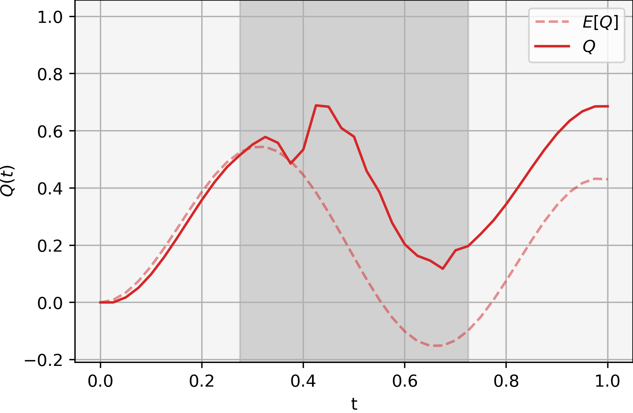
(a) Supply realization.

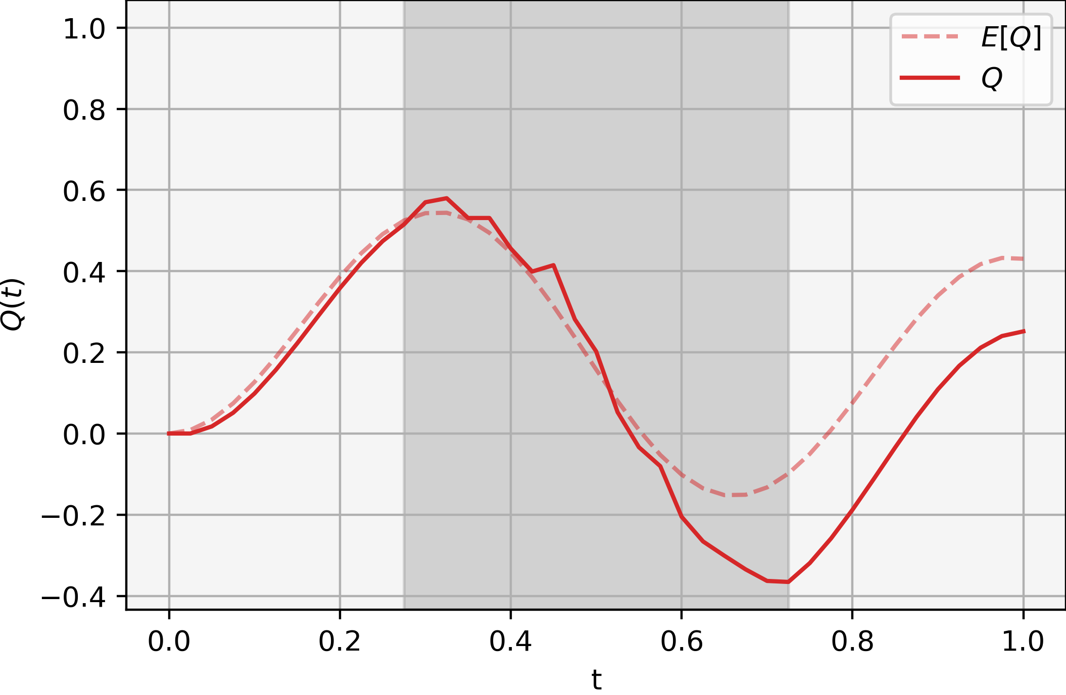
(b) Supply realization.

Figure 1: Two supply realizations of (20). The grey window highlights the times where noise operates.

We select $L(x,v)=\frac{1}{2}\left(x-1\right)^{2}+\frac{1}{2}v^{2}$ and $u_{T}\left(x\right)=\frac{1}{2e}\left(x-1\right)^{2}$. Figure 2 shows the evolution of the a posteriori estimate in Theorem 1. The balance error achieves enough accuracy and slightly oscillates with a decreasing tendency. The optimality error also exhibits a decreasing trend, but accuracy does not improve, suggesting testing other combinations of training and discretization parameters.

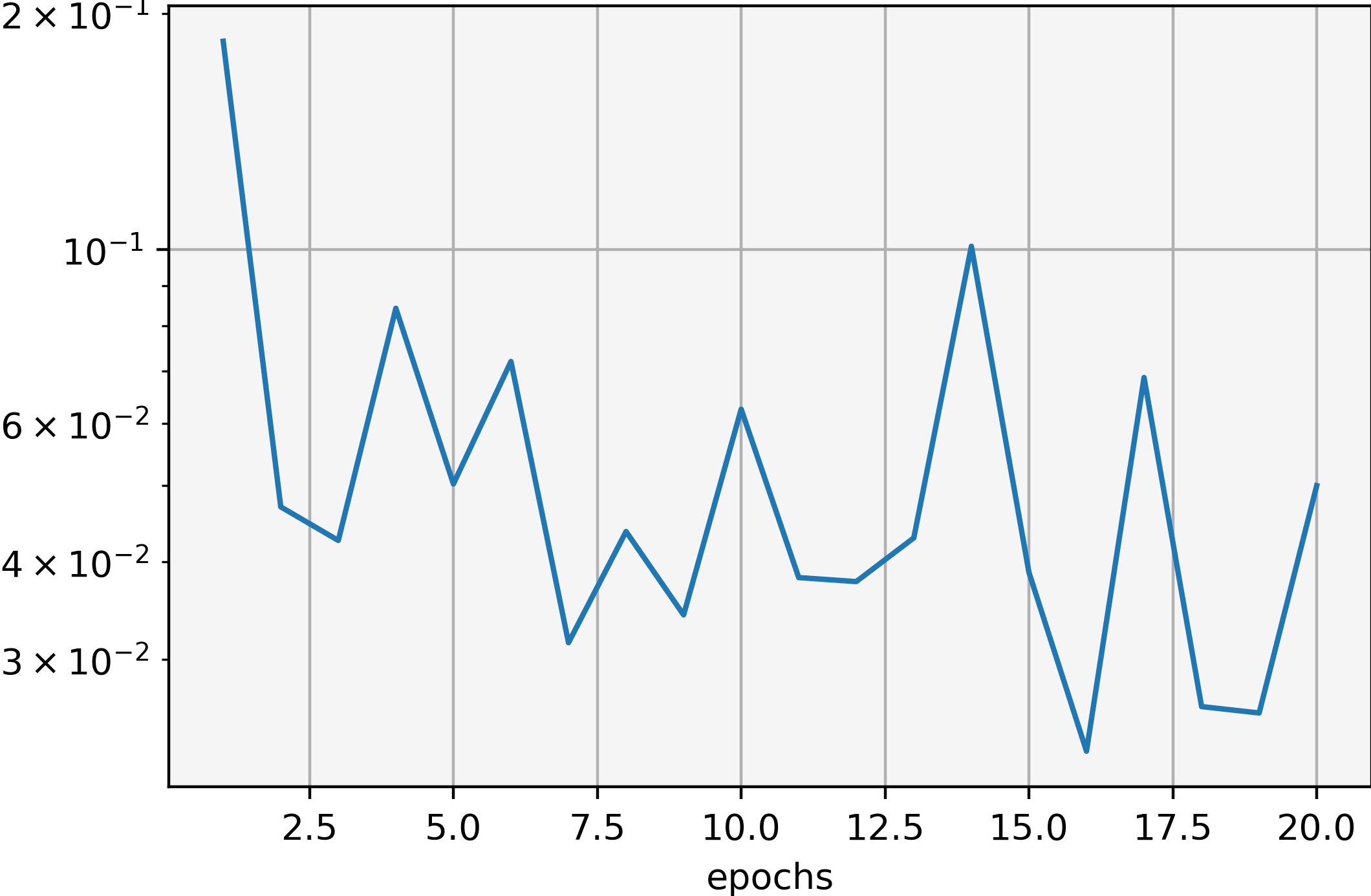
(a) $\mbox{MSE}(\epsilon_{B})$ (balance error).

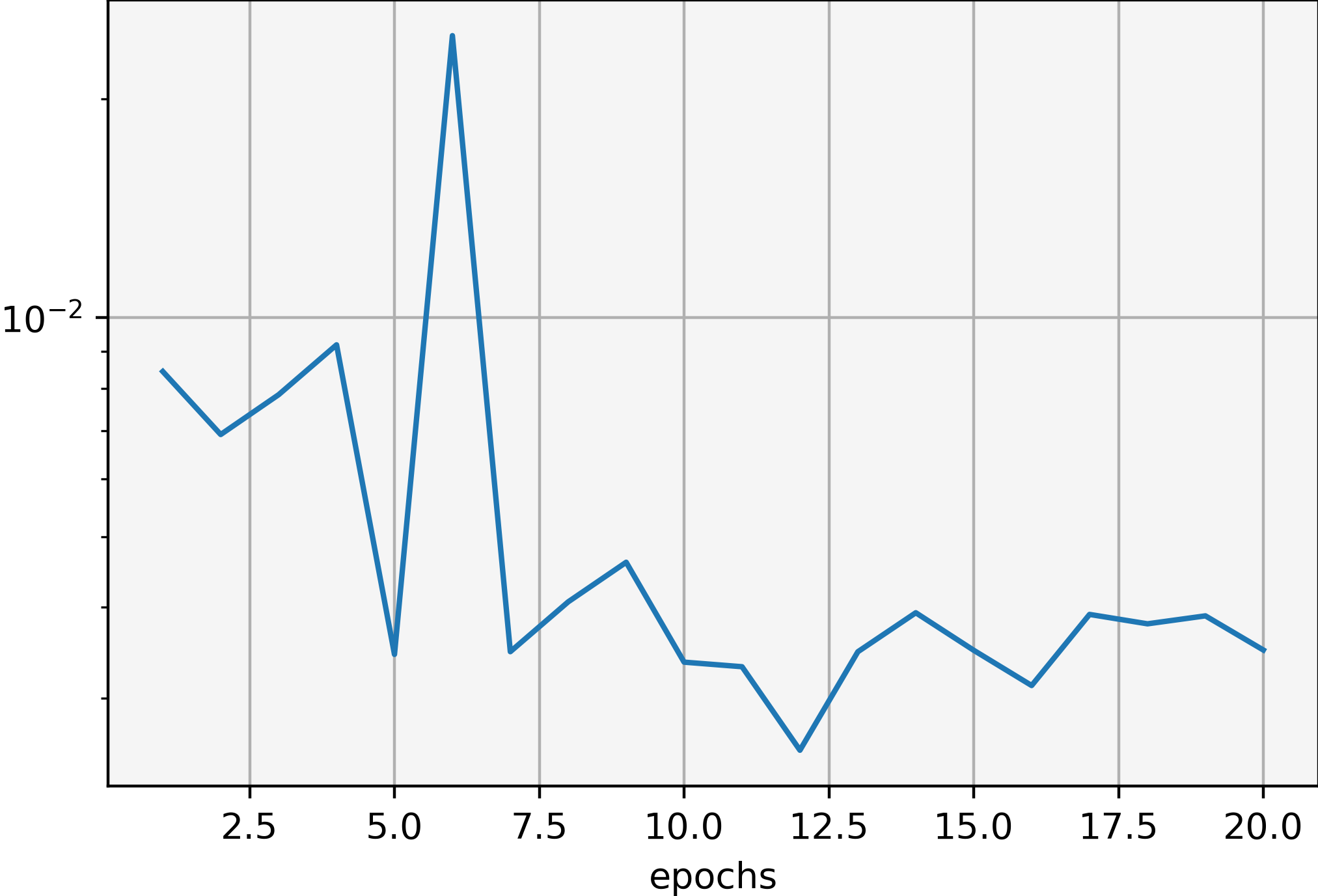
(b) $\mbox{MSE}(\epsilon_{H})$ (optimality error).

Figure 2: Evolution of the a posteriori estimates during training.

Furthermore, we use the analytic solution derived in [10] to verify the price approximation’s accuracy. In the linear-quadratic framework, the price follows from the SDE system

$$\begin{cases}{\rm d}Q(t)=(b^{S}(t)-Q_{t}){\rm d}t+\sigma^{S}(t){\rm d}W(t),\\ Q(0)=0,\\ {\rm d}\overline{X}(t)=Q(t){\rm d}t,\\ \overline{X}(0)=\overline{m}_{0},\\ {\rm d}\varpi(t)=\left(\overline{X}(t)-b^{S}(t)+Q(t)-1\right){\rm d}t\\ \quad\quad\quad\quad-\frac{a_{2}^{3}(t)+1}{a_{2}^{4}(t)+1}\sigma^{S}(t){\rm d}W(t),\\ \varpi(0)=w_{0}.\end{cases}$$ (21)

The value $w_{0}$ and the functions $a_{2}^{3}$ and $a_{2}^{4}$ are determined by a certain system of ordinary differential explicitly solvable. Figure 3 shows the corresponding price approximation and exact price (obtained from (21)) for the two supply realizations of Figure 1. The decreasing trend in the errors observed Figure 2 is reflected in the precise approximation observed in Figure 3. Notice the effect of the error in the time window $[0.25,0.75]$, which decreases, as expected, the accuracy of the approximation compared to the time region $[0,0.25]$, where no noise is applied.

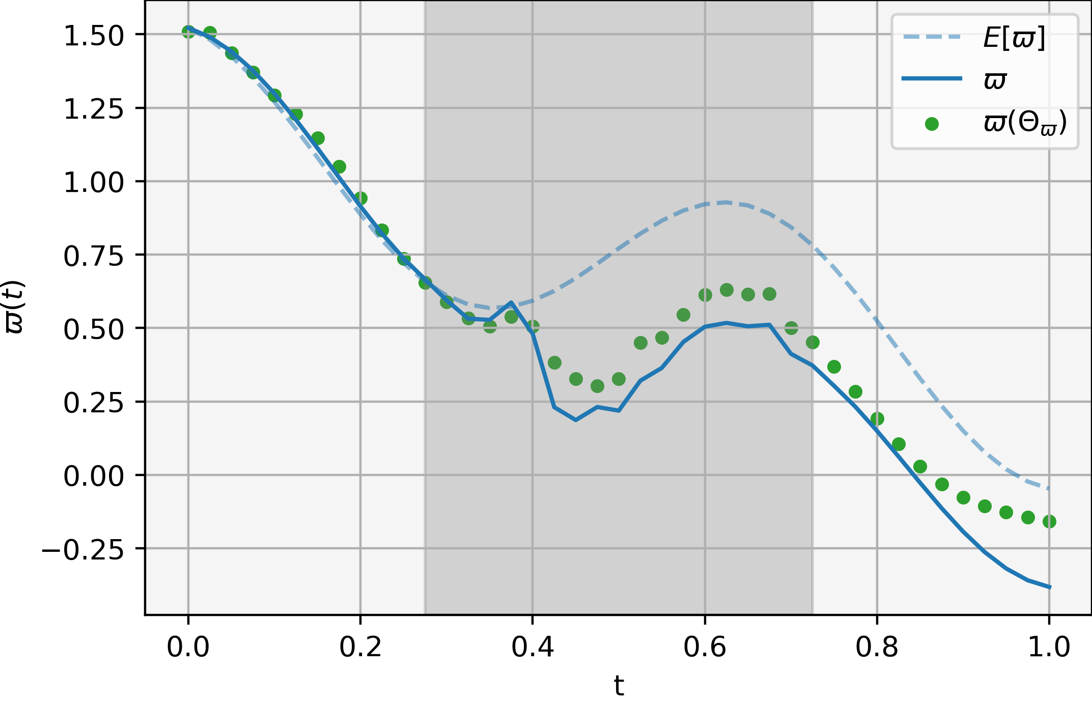
(a) Price realization for Figure 1(a).

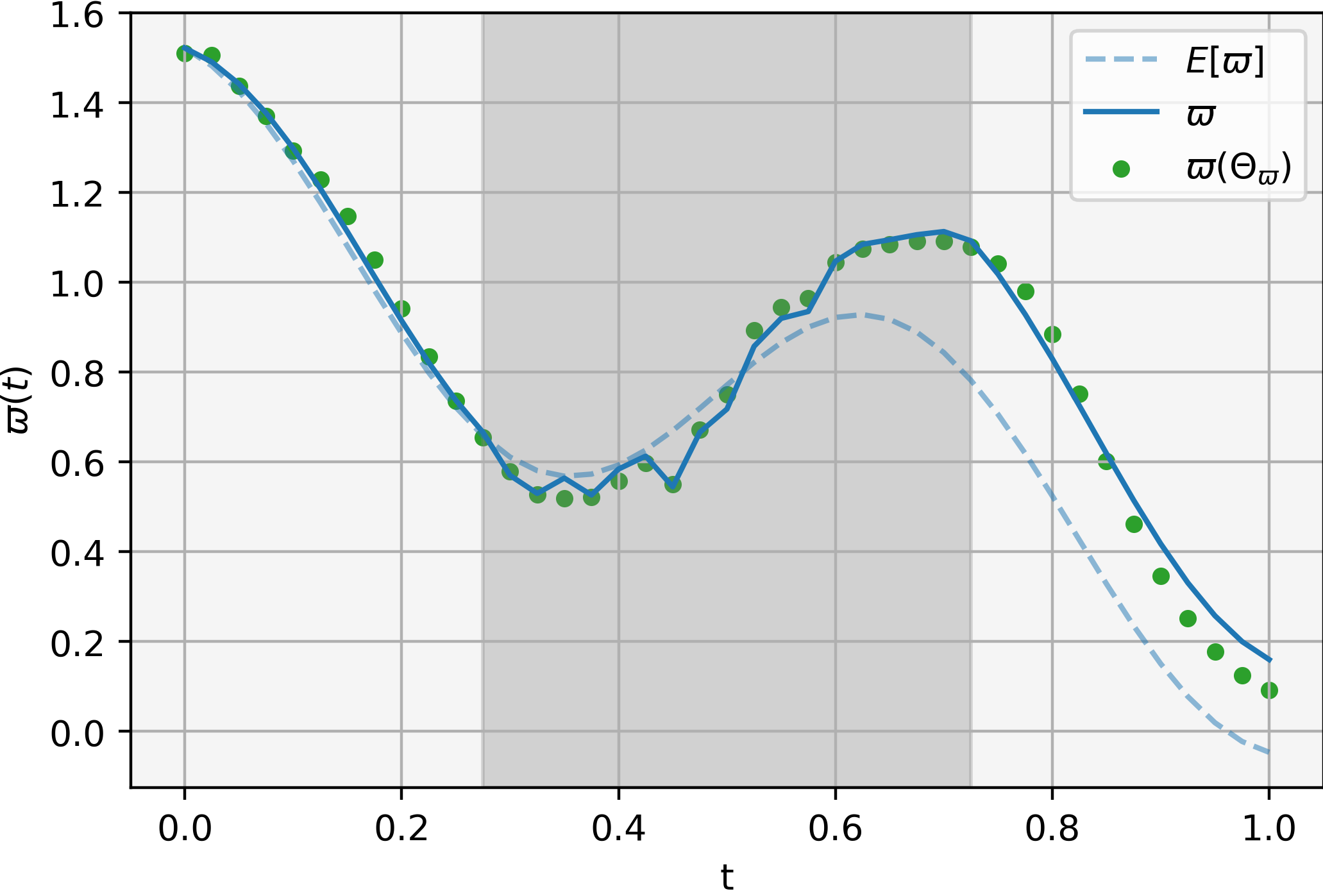
(b) Price realization for Figure 1(b).

Figure 3: Exact price and RNN approximation for Figure 1. The grey window highlights the times where noise operates.

As the figures show, the method has an excellent performance in approximating solutions in various noise regimes. Further research and refinements can enhance its efficiency, speed, and accuracy, leading to even more precise approximations in critical regions.

VI Conclusions and further directions

We extend the ML approach introduced in [8] for the deterministic setting to the common noise scenario, utilizing RNN architectures to represent non-anticipating controls. As in the deterministic case, our approach demonstrates good accuracy and performance.

Future research could explore method robustness concerning RNN and discretization parameter variations, addressing the trade-off between computational cost and accuracy. Comprehensive experiments may identify optimal RNN layer and neuron quantities for specific supply dynamics. Advanced coding methods could further reduce computational costs while maintaining or enhancing accuracy. Extensions could also accommodate additional noise sources, such as jump processes.

References

- [1] Y. Ashrafyan, T. Bakaryan, D. Gomes, and J. Gutierrez. The potential method for price-formation models. In 2022 IEEE 61st Conference on Decision and Control (CDC), pages 7565–7570, 2022.
- [2] C. Belak, D. Hoffmann, and F. T. Seifried. Continuous-time mean field games with finite state space and common noise. Applied Mathematics & Optimization, 84(3):3173–3216, 2021.
- [3] J.-D. Benamou and G. Carlier. Augmented lagrangian methods for transport optimization, mean field games and degenerate elliptic equations. Journal of Optimization Theory and Applications, 167(1):1–26, 2015.
- [4] E. Carlini and F. J. Silva. A fully discrete semi-lagrangian scheme for a first order mean field game problem. SIAM Journal on Numerical Analysis, 52(1):45–67, 2014.
- [5] R. Carmona and M. Laurière. Deep learning for mean field games and mean field control with applications to finance. To appear in Machine Learning And Data Sciences For Financial Markets (arXiv preprint arXiv:2107.04568), 2021.
- [6] G. Dayanikli and M. Lauriere. A machine learning method for stackelberg mean field games, 2023.
- [7] N. El Karoui, S. Peng, and M. C. Quenez. Backward stochastic differential equations in finance. Mathematical Finance, 7(1):1–71, 1997.
- [8] D. Gomes, J. Gutiérrez, and M. Laurière. Machine learning architectures for price formation models, 2022.
- [9] D. Gomes, J. Gutierrez, and R. Ribeiro. A mean field game price model with noise. Math. Eng., 3(4):Paper No. 028, 14, 2021.
- [10] D. Gomes, J. Gutierrez, and R. Ribeiro. A random-supply mean field game price model, 2021.
- [11] D. Gomes and J. a. Saúde. A Mean-Field Game Approach to Price Formation. Dyn. Games Appl., 11(1):29–53, 2021.
- [12] S. Hadikhanloo and F. J. Silva. Finite mean field games: Fictitious play and convergence to a first order continuous mean field game. Journal de Mathématiques Pures et Appliquées, 132:369–397, 2019.
- [13] J. Han and R. Hu. Recurrent neural networks for stochastic control problems with delay. Mathematics of Control, Signals, and Systems, 33:775–795, 2021.
- [14] C. Higham and D. Higham. Deep learning: an introduction for applied mathematicians. SIAM Review, 61(4):860–891, Nov. 2019.
- [15] M. Laurière, S. Perrin, M. Geist, and O. Pietquin. Learning mean field games: A survey, 2022.
- [16] M. Min and R. Hu. Signatured deep fictitious play for mean field games with common noise, 2021.
- [17] C. Mou, X. Yang, and C. Zhou. Numerical methods for mean field games based on gaussian processes and fourier features, 2021.