Learning from Integral Losses in Physics Informed Neural Networks

Abstract

This work proposes a solution for the problem of training physics informed networks under partial integro-differential equations. These equations require infinite or a large number of neural evaluations to construct a single residual for training. As a result, accurate evaluation may be impractical, and we show that naive approximations at replacing these integrals with unbiased estimates lead to biased loss functions and solutions. To overcome this bias, we investigate three types of solutions: the deterministic sampling approach, the double-sampling trick, and the delayed target method. We consider three classes of PDEs for benchmarking; one defining a Poisson problem with singular charges and weak solutions, another involving weak solutions on electro-magnetic fields and a Maxwell equation, and a third one defining a Smoluchowski coagulation problem. Our numerical results confirm the existence of the aforementioned bias in practice, and also show that our proposed delayed target approach can lead to accurate solutions with comparable quality to ones estimated with a large number of samples. Our implementation is open-source and available at https://github.com/ehsansaleh/btspinn.

1 Introduction

Physics Informed Neural Networks (PINNs) [23] can be described as solvers of a particular Partial Differential Equation (PDE). Typically, these problems consist of three defining elements. A sampling procedure selects a number of points for learning. Automatic differentiation is then used to evaluate the PDE at these points and define a residual. Finally, a loss function, such as the Mean Squared Error (MSE), is applied to these residuals, and the network learns the true solution by minimizing this loss through back-propagation and stochastic approximation. These elements form the basis of many methods capable of learning high-dimensional parameters. A wealth of existing work demonstrate the utility of this approach to solving a wide array of applications and PDE forms [16, 25, 15].

One particular problem in this area, is the prevalent assumption around our ability to accurately evaluate the PDE residuals for learning. In particular, many partial integro-differential forms may include an integral or a large summation within them. Weak solutions using the divergence or the curl theorems, or the Smoluchowski coagulation equation [28] are two examples of such forms. In such instances, an accurate evaluation of the PDE elements, even at a single point, can become impractical. Naive approximations, such as replacing integrals with unbiased estimates, can result in biased solutions, as we will show later. This work is dedicated to the problem of learning PINNs with loss functions containing a parametrized integral or large summation.

To tackle such challenging problems, this paper investigates three learning approaches: the deterministic sampling approach, the double-sampling trick, and the delayed target method. The deterministic sampling approach takes the integration stochasticity away. However, it optimizes a different objective and deterministic sampling schemes may not scale well to higher sampling dimensions. The double-sampling trick enjoys strong theoretical guarantees, but relies on a particular point sampling process and a squared loss form and may not be suitable for offline learning. Bootstrapping neural networks with delayed targets has already been studied in other contexts, such as the method of learning from Temporal Differences (TD-learning) in approximate dynamic programming [27]. Time and time again, TD-learning has proven preferable over the ordinary MSE loss minimization (known as the Bellman residual minimization) [24, 5, 31, 4]. Another example is the recent trend of semi-supervised learning, where teacher-student frameworks result in accuracy improvements of classification models by pseudo-labelling unlabelled examples for training [8, 22, 1, 14].

The main contributions of this work are: (1) we formulate the integral learning problem under a general framework and show the biased nature of standard approximated loss functions; (2) we present three techniques to solve such problems, namely the deterministic sampling approach, the double-sampling trick, and the delayed target method; (3) we detail an effective way of implementation for the delayed target method compared to a naive one; and (4) we compare the efficacy of the proposed solutions using numerical examples on a Poisson problem with singular charges, a Maxwell problem with magnetic fields, and a Smoluchowski coagulation problem.

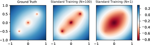
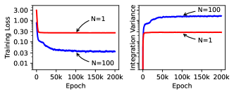
Figure 1: Training with the MSE loss under different sample sizes per-surface ($N$). The heatmaps show the analytical solution (left), the low-variance training with $N=100$ (middle), and the high-variance training with $N=1$ (right). The smaller the $N$, the more biased the training objective becomes towards finding smoother solutions. The right panel shows the training curves; the training loss and the integration variance represent $\hat{\mathcal{L}}_{\theta}(x)$ and $\mathbb{V}_{P(x^{\prime}|x)}[g_{\theta}(x^{\prime})]$ in Equation (15), respectively. For $N=1$, the training loss seems to be floored at the same value as the integration variance (i.e., approximately $0.3$). However, with $N=100$, the model produces better solutions, lower training losses, and higher integration variances.

2 Problem Formulation

Consider a typical partial integro-differential equation

$$f_{\theta}(x):=\mathbb{E}_{P(x^{\prime}|x)}[g_{\theta}(x^{\prime})]+y.$$ (1)

The $f_{\theta}(x)$ and $g_{\theta}(x^{\prime})$ are parametrized, and $y$ includes all the non-parametrized terms in the PDE. The right side of the equation serves as the target value for $f_{\theta}(x)$. For notation simplicity, we assume a fixed value for $x$ in the remainder of the manuscript. However, all analyses are applicable to randomized $x$ without any loss of generality. Equation (1) is a general, yet concise, form for expressing partial integro-differential equations. To motivate, we will express two examples.

Algorithm 1 Regularized delayed target method for training integro-differential PINNs

0:  The initial parameter values $\theta_{0}$, learning rate $\eta$, Polyak averaging rate $\gamma$, target sample size $N$, and the target regularization weight $\lambda$.

1:  Initialize the main and target parameters: $\theta,\theta_{\text{Target}}\leftarrow\theta_{0}$.

2:  for $k=1,2,\ldots$ do

3:     Compute the $f_{\theta}(x)$ term using the main parameters.

4:     Sample the $\{x^{\prime}_{i}\}_{i=1}^{N}$ set from $P(\{x^{\prime}_{i}\}|x)$.

5:     Compute the target $\frac{1}{N}\sum_{i=1}^{N}g_{\theta^{\text{Target}}}(x^{\prime}_{i})+y$ using the target parameters $\theta_{\text{Target}}$.

6:     Construct the main loss: $\hat{\mathcal{L}}_{\theta}^{\text{DT}}=\big{(}f_{\theta}(x)-\frac{1}{N}\sum_{i=1}^{N}g_{\theta^{\text{Target}}}(x^{\prime}_{i})-y\big{)}^{2}.$

7:     Construct the target regularization loss: $\hat{\mathcal{L}}_{\theta}^{\text{R}}=(f_{\theta}(x)-f_{\theta^{\text{Target}}}(x))^{2}.$

8:     Compute the total loss $\hat{\mathcal{L}}_{\theta}^{\text{DT}\text{R}}=\hat{\mathcal{L}}^{\text{DT}}_{\theta}(x)+\lambda\hat{\mathcal{L}}_{\theta}^{\text{R}}.$

9:     Perform a gradient descent step on $\theta$: $\theta\leftarrow\theta-\eta\nabla_{\theta}\hat{\mathcal{L}}_{\theta}^{\text{DT}\text{R}}.$

10:     Update the target parameters using Polyak averaging: $\theta^{\text{Target}}\leftarrow\gamma\theta^{\text{Target}}+(1-\gamma)\theta.$

11:  end for

Example 1

The Poisson problem is to solve the system $\nabla^{2}U=\rho$ for $U$ given a charge function $\rho$. This is equivalent to finding a solution for the system

$$E=\nabla U,\qquad\nabla\cdot E=\rho.$$ (2)

A weak solution can be obtained through enforcing the divergence theorem over many volumes:

$$\int_{\partial\Omega}E\cdot\hat{n}\quad\mathrm{d}S=\iint_{\Omega}\nabla\cdot E\quad\mathrm{d}V,$$ (3)

where $\hat{n}$ is the normal vector perpendicular to $\mathrm{d}S$. The weak solutions can be preferable over the strong ones when dealing with singular or sparse $\rho$ charges.

To solve this system, we parametrize $E(x)$ as the gradient of a neural network predicting the $U$ potentials. To convert this into the form of Equation (1), we replace the left integral in Equation (3) with an arbitrarily large Riemann sum and write

$$\int_{\partial\Omega}E\cdot\hat{n}\quad\mathrm{d}S=\frac{A}{M}\sum_{i=1}^{M}E_{\theta}(x_{i})\cdot\hat{n}_{i},$$ (4)

where $A=\int_{\partial\Omega}1\text{ d}S$ is the surface area and the $x_{i}$ samples are uniform on the surface. To convert this system into the form of Equation (1), we then define

$$x:=x_{1}, \qquad f_{\theta}(x):=\frac{A}{M}E_{\theta}(x)\cdot\hat{n}_{1},\qquad x^{\prime}\sim\text{Unif}(\{x_{i}\}_{i=2}^{M}),$$

$$g_{\theta}(x_{i}) :=-\frac{A(M-1)}{M}E_{\theta}(x_{i})\cdot\hat{n}_{i},\qquad y:=\iint_{\Omega}\rho\mathrm{d}V.$$ (5)

Example 2

In static electromagnetic conditions, one of the Maxwell Equations, the Ampere circuital law, is to solve the system $\nabla\times A=B$, $\nabla\times B=J$ for $A$ given the current density $J$ in the 3D space (we assumed a unit physical coefficient for simplicity). Here, $B$ represents the magnetic field and $A$ denotes the magnetic potential vector. A weak solution for this system can be obtained through enforcing the Stokes theorem over many volumes:

$$\int_{\partial\Omega}\nabla\times A\cdot\mathrm{d}\mathbf{l}=\iint_{\Omega}J\cdot\mathrm{d}S,$$ (6)

where $\mathrm{d}S$ is an infinitesimal surface normal vector. Just like the Poisson problem, the weak solutions can be preferable over the strong ones when dealing with singular inputs, and this equation can be converted into the form of Equation (1) similarly.

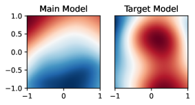
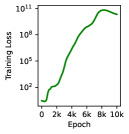
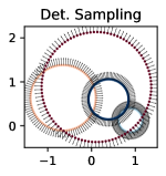
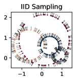
aaaaaa

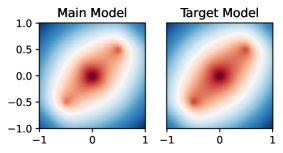
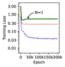
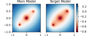
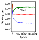
Figure 2: Training the same problem as in Figure 1 with delayed targets and $N=1$. The top left panel shows a diverged training with $M=100$ in Equation (24). The lower left panel corresponds to $M=10$, which has a converging training curve even though producing an overly smooth solution. In the lower right panel, we set $\lambda=1$ which allowed setting the simulated $M$ as $1000$ while maintaining a stable training loss. In each panel, the left and right heatmaps show the main and the target model predictions, respectively, and the right plots show the training curves. The green curves show the training loss for the delayed target method, and the standard training curves with $N=1$ and $100$ are also shown using dotted red and blue lines for comparison, respectively. The top right panel shows an example of deterministic vs. i.i.d. sampling of the surface points $\{x^{\prime}_{i}\}_{i=1}^{N}$ in the Poisson problem. For each sampled sphere, the surface points and their normal vectors are shown with $N=100$ samples. With deterministic sampling, the points are evenly spaced to cover the sampling domain.

Example 3

The Smoluchowski coagulation equation simulates the evolution of particles into larger ones, and is described as

$$\frac{\partial\rho(x,t)}{\partial t}= \int_{0}^{x}K(x-x^{\prime},x^{\prime})\rho(x-x^{\prime},t)\rho(x^{\prime},t)\mathrm{d}x^{\prime}-\int_{0}^{\infty}K(x,x^{\prime})\rho(x,t)\rho(x^{\prime},t)\mathrm{d}x^{\prime},$$ (7)

where $K(x,x^{\prime})$ is the coagulation kernel between two particles of size $x$ and $x^{\prime}$. The particle sizes $x$ and $x^{\prime}$ can be generalized into vectors, inducing a higher-dimensional PDE to solve. To solve this problem, we parametrize $\rho(x,t)$ as the output of a neural network with parameters $\theta$ and write

$$f_{\theta}(x):=\frac{\partial\rho_{\theta}(x,t)}{\partial t},\qquad g_{\theta}^{(1)}(x^{\prime}):=A_{1}K(x-x^{\prime},x^{\prime})\rho_{\theta}(x-x^{\prime},t)\rho_{\theta}(x^{\prime},t),$$

$$g_{\theta}^{(2)}(x^{\prime}) :=A_{2}K(x,x^{\prime})\rho_{\theta}(x,t)\rho_{\theta}(x^{\prime},t).$$ (8)

The $x^{\prime}$ values in both $g_{\theta}^{(1)}$ and $g_{\theta}^{(2)}$ are sampled from their respective uniform distributions, and $A_{1}$ and $A_{2}$ are used to normalize the uniform integrals into expectations. Finally, $y=0$ and we can define $g_{\theta}(x^{\prime})$ in a way such that

$$\mathbb{E}_{x^{\prime}}[g_{\theta}(x^{\prime})]:=\mathbb{E}_{x^{\prime}}[g_{\theta}^{(1)}(x^{\prime})]+\mathbb{E}_{x^{\prime}}[g_{\theta}^{(2)}(x^{\prime})].$$ (9)

The standard way to solve systems such as Examples 1, 2, and 3 with PINNs, is to minimize the following mean squared error (MSE) loss [23, 9]:

$$\mathcal{L}_{\theta}(x):=\big{(}f_{\theta}(x)-\mathbb{E}_{P(x^{\prime}|x)}[g_{\theta}(x^{\prime})]-y\big{)}^{2}.$$ (10)

Since computing exact integrals may be impractical, one may contemplate replacing the expectation in Equation (10) with an unbiased estimate, as implemented in NVIDIA’s Modulus package [21]. This prompts the following approximate objective:

$$\hat{\mathcal{L}}_{\theta}(x):=\mathbb{E}_{\{x^{\prime}_{i}\}_{i=1}^{N}}\bigg{[}\big{(}f_{\theta}(x)-\frac{1}{N}\sum_{i=1}^{N}g_{\theta}(x^{\prime}_{i})-y\big{)}^{2}\bigg{]}.$$ (11)

We therefore analyze the approximation error:

$$\hat{\mathcal{L}}_{\theta}(x)= \mathbb{E}_{\{x^{\prime}_{i}\}}\bigg{[}\bigg{(}\big{(}f_{\theta}(x)-\mathbb{E}_{x^{\prime\prime}}[g_{\theta}(x^{\prime\prime})]-y\big{)}+\big{(}\mathbb{E}_{x^{\prime\prime}}[g_{\theta}(x^{\prime\prime})]-\frac{1}{N}\sum_{i=1}^{N}g_{\theta}(x^{\prime}_{i})\big{)}\bigg{)}^{2}\bigg{]}.$$ (12)

By decomposing the squared sum, we get

$$\hat{\mathcal{L}}_{\theta}(x)=\phantom{a} \mathbb{E}_{\{x^{\prime}_{i}\}}\big{[}\big{(}\big{(}f_{\theta}(x)-\mathbb{E}_{x^{\prime\prime}}[g_{\theta}(x^{\prime\prime})]-y\big{)}^{2}\big{]}+\mathbb{E}_{\{x^{\prime}_{i}\}}\big{[}(\mathbb{E}_{x^{\prime\prime}}[g_{\theta}(x^{\prime\prime})]-\frac{1}{N}\sum_{i=1}^{N}g_{\theta}(x^{\prime}_{i}))^{2}\big{]}$$

$$-2\mathbb{E}_{\{x^{\prime}_{i}\}}\big{[}\big{(}f_{\theta}(x)-\mathbb{E}_{x^{\prime\prime}}[g_{\theta}(x^{\prime\prime})]-y\big{)}\big{(}\mathbb{E}_{x^{\prime\prime}}[g_{\theta}(x^{\prime\prime})]-\frac{1}{N}\sum_{i=1}^{N}g_{\theta}(x^{\prime}_{i})\big{)}\big{]}.$$ (13)

Since $\mathbb{E}_{x^{\prime\prime}}[g_{\theta}(x^{\prime\prime})]=\mathbb{E}_{\{x^{\prime}_{i}\}}[\frac{1}{N}\sum_{i=1}^{N}g_{\theta}(x^{\prime}_{i})]$, the last term in Equation (2) is zero, and we have

$$\hat{\mathcal{L}}_{\theta}(x)=\mathcal{L}_{\theta}(x)+\mathbb{V}_{P(\{x^{\prime}_{i}\}|x)}[\frac{1}{N}\sum_{i=1}^{N}g_{\theta}(x^{\prime}_{i})].$$ (14)

If the $x^{\prime}_{i}$ are sampled in an i.i.d. manner, Equation (14) simplifies further to

$$\hat{\mathcal{L}}_{\theta}(x)=\mathcal{L}_{\theta}(x)+\frac{1}{N}\mathbb{V}_{P(x^{\prime}|x)}[g_{\theta}(x^{\prime})].$$ (15)

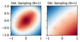
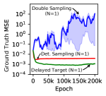
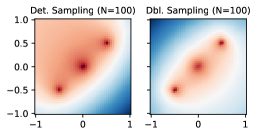
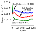
Figure 3: The results of the deterministic and double sampling techniques on the Poisson problem. The left plots demonstrate the solutions with $N=1$, while the right plots show the solutions with $N=100$. The training curves represent the mean squared error to the analytical solution vs. the training epochs. With $N=1$, the double sampling trick exhibits divergence in training, and the deterministic sampling process yields overly-smooth functions similar to the standard solution in Figure 1. However, with $N=100$, both the deterministic and double-sampling approaches exhibit improvements. According to the training curves, the delayed target method with $N=1$ yields the best solutions in this problem.

The induced excess variance in Equation (15) can bias the optimal solution. As a result, optimizing the approximated loss will prefer smoother solutions over all $\{x^{\prime}_{i}\}_{i=1}^{N}$ samples. It is worth noting that this bias is mostly harmful due to its parametrized nature; the only link through which this bias can offset the optimal solution is its dependency on $\theta$. This is in contrast to any non-parametrized stochasticity in the $y$ term of Equation (10). Non-parameterized terms cannot offset the optimal solutions, since stochastic gradient descent methods are indifferent to them.

3 Proposed Solutions

Based on Equation (15), the induced bias in the solution has a direct relationship with the stochasticity of the conditional distribution $P(x^{\prime}|x)$. If we were to sample the $(x,x^{\prime})$ pairs deterministically, the excess variance in Equation (15) would disappear. However, this condition is satisfied only by modifying the problem conditions. Next, we introduce three preliminary solutions to this problem: the deterministic sampling strategy, the double-sampling trick, and the delayed target method.

The deterministic sampling strategy: One approach to eliminate the excess variance term in Equation (14), is to sample the $\{x^{\prime}_{i}\}_{i=1}^{N}$ set in a way that $P(\{x^{\prime}_{i}\}|x)$ would be a point mass distribution at a fixed set $\mathbb{A}_{x}$. This way, $P(\{x^{\prime}_{i}\}|x)$ yields a zero excess variance: $\mathbb{V}[\frac{1}{N}\sum_{i=1}^{N}g_{\theta}(\mathbb{A}_{x}^{(i)})]=0$. This induces the following deterministic loss.

$$\hat{\mathcal{L}}^{\text{DET}}_{\theta}(x):=\bigg{(}f_{\theta}(x)-\frac{1}{N}\sum_{i=1}^{N}g_{\theta}(\mathbb{A}_{x}^{(i)})-y\bigg{)}^{2}.$$ (16)

Although this approach removes the excess variance term in Equation (14) thanks to its deterministic nature, it biases the optimization loss by re-defining it: $\mathcal{L}_{\theta}(x)\neq\hat{\mathcal{L}}^{\text{DET}}_{\theta}(x)$. The choice of the $\mathbb{A}_{x}$ set can influence the extent of this discrepancy. One reasonable choice is to evenly space the $N$ samples to cover the entire sampling domain as uniformly as possible. For a demonstration, Figure 2 shows a number of example sets used for applying the divergence theorem to the Poisson problem. Of course, this sampling strategy can be impractical in high-dimensional spaces, as the number of samples needed to cover the entire sampling domain grows exponentially with the sampling space dimension.

The double-sampling trick: If we have two independent $x^{\prime}$ samples, namely $x^{\prime}_{1}$ and $x^{\prime}_{2}$, we can replace the objective in Equation (11) with

$$\hat{\mathcal{L}}^{\text{DBL}}_{\theta}(x)=\mathbb{E}_{x^{\prime}_{1},x^{\prime}_{2}\sim P(x^{\prime}|x)}\bigg{[}\big{(}f_{\theta}(x)-g_{\theta}(x^{\prime}_{1})-y\big{)}\cdot\big{(}f_{\theta}(x)-g_{\theta}(x^{\prime}_{2})-y\big{)}\bigg{]}.$$ (17)

It is straightforward to show that $\hat{\mathcal{L}}^{\text{DBL}}_{\theta}(x)=\mathcal{L}_{\theta}(x)$; the uncorrelation between $g_{\theta}(x^{\prime}_{1})$ and $g_{\theta}(x^{\prime}_{2})$ will remove the induced bias on average. However, this approach requires the access to two i.i.d. samples, which may not be plausible in many sampling schemes. In particular, Monte-Carlo samplings used in reinforcement learning do not usually afford the learning method with freedom to choose multiple next samples or being able to reset to a previous state. Besides reinforcement learning, offline learning using a given collection of samples may make this approach impractical.

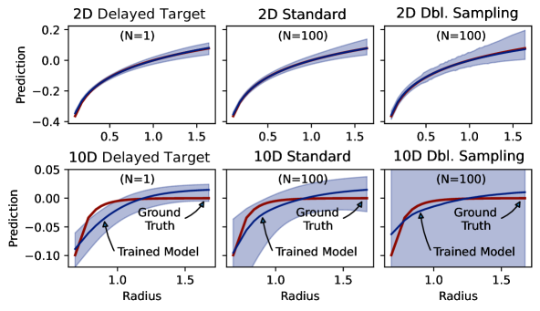
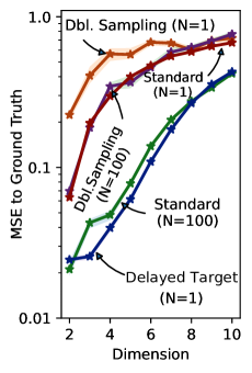
Figure 4: The solution and performance curves in higher-dimensional Poisson problems. The left panel shows the solution curves for the delayed target $(N=1)$, the standard $(N=100)$, and the double-sampling $(N=100)$ methods. The top and the bottom rows show 2- and 10-dimensional problems, respectively. In these problems, a single charge is located at the origin, so that the analytical solution is a function of the evaluation point radii $\|x\|$. The horizontal axis shows the evaluation point radii, and covers 99% of points within the training volumes. The right chart is a performance curve against the problem dimension (lower is better). The normalized MSE values were shown to be comparable. These results suggest that (1) higher dimensions make the problem challenging, and (2) delayed targeting with $N=1$ is comparable to standard trainings with $N=100$.

The delayed target method: This approach replaces the objective in Equation (11) with

$$\mathcal{L}^{\text{DT}}_{\theta}(x)=\mathbb{E}_{P(x^{\prime}|x)}\bigg{[}\big{(}f_{\theta}(x)-g_{\theta^{*}}(x^{\prime})-y\big{)}^{2}\bigg{]},$$ (18)

where we have defined $\theta^{*}:=\operatorname*{arg\,min}_{\tilde{\theta}}\mathcal{L}_{\tilde{\theta}}(x)$. Assuming a complete function approximation set $\Theta$ (where $\theta\in\Theta$), we know that $\theta^{*}$ satisfies Equation (1) at all points. Therefore, we have

$$\nabla_{\theta}\mathcal{L}_{\theta}(x)\big{|}_{\theta=\theta^{*}}=\nabla_{\theta}\mathcal{L}^{\text{DT}}_{\theta}(x)\big{|}_{\theta=\theta^{*}}=0.$$ (19)

Therefore, we can claim

$$\theta^{*}=\operatorname*{arg\,max}_{\theta}\mathbb{E}_{x}[\mathcal{L}^{\text{DT}}_{\theta}(x)]=\operatorname*{arg\,min}_{\theta}\mathbb{E}_{x}[\mathcal{L}_{\theta}(x)].$$ (20)

In other words, optimizing Equation (18) should yield the same solution as optimizing the true objective $\mathcal{L}_{\theta}(x)$ in Equation (10). Of course, finding $\theta^{*}$ is as difficult as solving the original problem. The simplest heuristic replaces $\theta^{*}$ with a supposedly independent, yet identically valued, version of the latest $\theta$ named $\theta^{\text{Target}}$, hence the delayed, detached, and bootstrapped target naming conventions:

$$\hat{\mathcal{L}}^{\text{DT}}_{\theta}(x)=\mathbb{E}_{P(\{x^{\prime}_{i}\}|x)}\bigg{[}\big{(}f_{\theta}(x)-\frac{1}{N}\sum_{i=1}^{N}g_{\theta^{\text{Target}}}(x^{\prime}_{i})-y\big{)}^{2}\bigg{]}.$$ (21)

Our hope would be for this approximation to improve as well as $\theta$ over training. The only practical difference between implementing this approach and minimizing the loss in Equation (10) is to use an incomplete gradient for updating $\theta$ by detaching the $g(x^{\prime})$ node from the computational graph in the automatic differentiation software. This naive implementation of the delayed target method can lead to divergence in optimization, as we will show in Section 4 with numerical examples (i.e., Figure 2). Here, we introduce two mitigation factors contributing to the stabilization of such a technique.

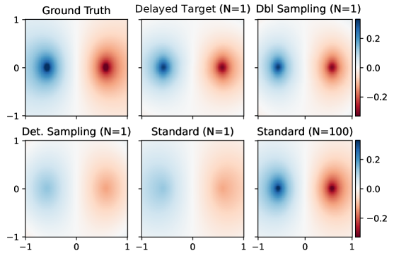
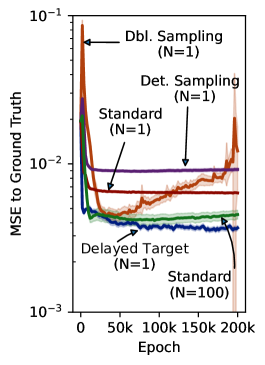
Figure 5: The solution heatmaps and the training curves for different methods to the Maxwell problem. In the left panel, we show a single component of the magnetic potentials ($A_{z}$) in a 2D slice of the training space with $z=0$ for visual comparison. In the right plot, we show the training curves. The results suggest that (1) the standard and deterministic trainings with $N=1$ produce overly smooth solutions, and (2) delayed targeting with $N=1$ is comparable to standard trainings with $N=100$.

Moving target stabilization

One disadvantage of the aforementioned technique is that it does not define a global optimization objective; even the average target for $f_{\theta}(x)$ (i.e., $\mathbb{E}\big{[}g_{\theta^{\text{Target}}}(x^{\prime})\big{]}+y$) changes throughout the training. Therefore, a naive implementation can risk training instability or even divergence thanks to the moving targets.

To alleviate the fast moving targets issue, prior work suggested fixing the target network for many time-steps [19]. This causes the training trajectory to be divided into a number of episodes, where the target is locally constant and the training is therefore locally stable in each episode. Alternatively, this stabilization can be implemented continuously using Polyak averaging; instead of fixing the target network for a window of $T$ steps, the target parameters $\theta^{\text{Target}}$ can be updated slowly with the rule

$$\theta^{\text{Target}}\leftarrow\gamma\theta^{\text{Target}}+(1-\gamma)\theta.$$ (22)

This exponential moving average defines a corresponding stability window of $T=O(1/(1-\gamma))$.

Prior imposition for highly stochastic targets

In certain instances, the target $\frac{1}{N}\sum_{i=1}^{N}g_{\theta^{\text{Target}}}(x^{\prime}_{i})+y$ in Equation (18) can be excessively stochastic, leading to divergence in the training of the delayed target model. In particular, based on the settings defined in Equation (2) for the Poisson problem, we can write $g_{\theta}(x_{i})=(M-1)f_{\theta}(x_{i})$. Therefore, we can analyze the target variance as

$$\mathbb{V}_{\{x^{\prime}_{i}\}_{i=1}^{N}}\big{[}\frac{1}{N}\sum_{i=1}^{N}g_{\theta^{\text{Target}}}(x^{\prime}_{i})+y\big{]}=\frac{(M-1)^{2}}{N}\mathbb{V}_{\{x^{\prime}_{i}\}_{i=1}^{N}}[f_{\theta^{\text{Target}}}(x^{\prime}_{i})]+\mathbb{V}[y].$$ (23)

Ideally, $M\rightarrow\infty$ in order for Equation (4) to hold. Setting arbitrarily large $M$ will lead to unbounded target variances in Equation (23), which can slow down the convergence of the training or result in divergence. In particular, such unbounded variances can cause the main and the target models to drift away from each other leading to incorrect solutions.

One technique to prevent this drift, is to impose a Bayesian prior on the main and the target models. Therefore, to discourage this divergence phenomenon, we regularize the delayed target objective in Equation (24) and replace it with

$$\hat{\mathcal{L}}_{\theta}^{\text{DT}\text{R}}:=\hat{\mathcal{L}}^{\text{DT}}_{\theta}(x)+\lambda\cdot(f_{\theta}(x)-f_{\theta^{\text{Target}}}(x))^{2}.$$ (24)

A formal description of the regularized delayed targeting process is given in Algorithm 1, which covers both of the moving target stabilization and the Bayesian prior imposition.

4 Experiments

                      

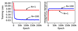
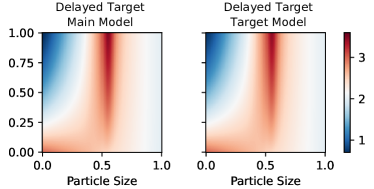
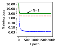
Figure 6: Training results on the Smoluchowski coagulation problem. The top left panel shows the ground truth solution, along with the standard $N=100$ and $N=1$ solution heatmaps minimizing the $\hat{\mathcal{L}}_{\theta}(x)$ in Equation (15). The training loss and the integration variance represent the $\hat{\mathcal{L}}_{\theta}(x)$ and $\mathbb{V}_{P(x^{\prime}|x)}[g_{\theta}(x^{\prime})]$ quantities in Equation (15). The top right figure shows the training curve for both of the standard trainings. The bottom left panel shows the delayed target solution heatmaps using $N=1$ sample with its training curve next to it.

We examine solving three problems. First, we solve a Poisson problem with singular charges using the divergence theorem as a proxy for learning. Figures 1, 2, and 3 define a 2D Poisson problem with three unit Dirac-delta charges at $[0,0]$, $[-0.5,-0.5]$, and $[0.5,0.5]$. We also study higher-dimensional Poisson problems with a unit charge at the origin in Figure 4. Our second example looks at finding the magnetic potentials and fields around a current circuit, which defines a singular current density profile $J$. Finally, to simulate particle evolution dynamics, we consider a Smoluchowski coagulation problem where particles evolve from an initial density. We designed the coagulation kernel $K$ to induce non-trivial solutions in our solution intervals. We employ a multi-layer perceptron as our deep neural network, using 64 hidden neural units in each layer, and the $\tanh$ activation function. We trained our networks using the Adam [12] variant of the stochastic gradient descent algorithm under a learning rate of $0.001$. For a fair comparison, we afforded each method 1000 point evaluations for each epoch. Due to space limitations, a wealth of ablation studies with more datasets and other experimental details were left to the supplementary material.

The Poisson problem with singular charges

To show the solution bias, we first train two models: one with $N=100$ samples per sphere, and another one with only $N=1$ sample per sphere. These models represent a baseline for later comparisons. Based on Equation (15), the induced solution bias should be lower in the former scenario. Figure 1 shows the solution defined by these models along with the analytical solution and their respective training curves. The model trained with high estimation variance derives an overly smooth solution. We hypothesize that this is due to the excess variance in the loss. This hypothesis is confirmed by matching the training loss and the excess variance curves; the training loss of the model with $N=1$ is lower bounded by its excess variance, although it successfully finds a solution with smaller excess variance than the $N=100$ model. An alternative capable of producing similar quality solutions with only $N=1$ samples would be ideal.

To investigate the effect of highly stochastic targets on delayed target models, Figure 2 shows the training results with both $M=100$ and $M=10$. The former is unstable, while the latter is stable; this confirms the influence of $M$ in the convergence behavior of the delayed target trainings. Furthermore, when this divergence happens, a clear drift between the main and the target models can be observed. Figure (2) shows that imposing the Bayesian prior of Equation (24) can lead to training convergence even with a larger $M=1000$, which demonstrates the utility of our proposed solution.

We also investigated the performance of the deterministic and double-sampling techniques in this problem. Figure 3 shows these results when $N=1$ and $N=100$ samples are used for integral estimation. With $N=1$, the training with the deterministic sampling approach is stable and yields similar results to those seen in Figure (1). The double-sampling trick, on the other hand, exhibits unstable trainings and sub-optimal solutions. We suspect that (a) the singular nature of the analytical solution, and (b) the stochasticity profile of the training loss function $\hat{\mathcal{L}}^{\text{DBL}}_{\theta}(x)$ in Equation (17) are two of the major factors contributing to this outcome. With $N=100$, both the deterministic and double-sampling trainings yield stable training curves and better solutions. This suggests that both methods can still be considered as viable options for training integro-differential PINNs, conditioned on that the specified $N$ is large enough for these methods to train stably and well.

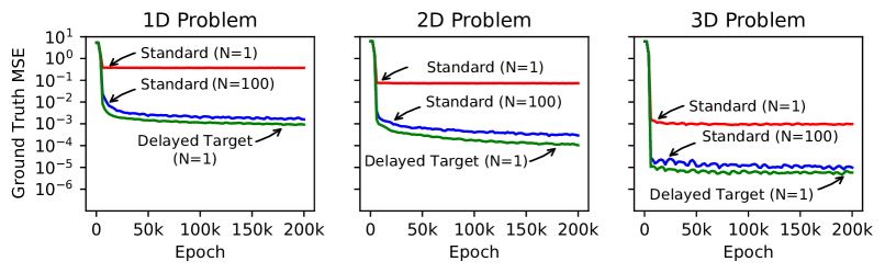
Figure 7: The solution mean squared error to the ground truth in the 1, 2, and 3-dimensional Smoluchowski coagulation problem. The vertical axis shows the solution error, and the horizontal axis shows the training epochs. The standard solutions were trained by the ordinary MSE loss $\mathcal{L}_{\theta}(x)$ in Equation (10) with $N=1$ and $N=100$ samples. The delayed target solution used $N=1$ sample, yet produced slightly better results than the standard method with $N=100$.

The regularized delayed target training with $N=1$ sample is also shown in the training curves of Figure 3 for easier comparison. The delayed target method yields better performance than the deterministic or double-sampling in this problem. This may seemingly contradict the fact that the double-sampling method enjoys better theoretical guarantees than the delayed target method, since it optimizes a complete gradient. However, our results are consistent with recent findings in off-policy reinforcement learning; even in deterministic environments where the application of the double-sampling method can be facilitated with a single sample, incomplete gradient methods (e.g., TD-learning) may still be preferable over the full gradient methods (e.g., double-sampling) [24, 5, 31, 4]. Intuitively, incomplete gradient methods detach parts of the gradient, depriving the optimizer from exercising full control over the decent direction and make it avoid over-fitting. In other words, incomplete gradient methods can be viewed as a middle ground between zero-order and first-order optimization, and may be preferable over both of them.

Figure 4 also studies the effect of problem dimensionality on our methods. The results confirm that the problem becomes significantly more difficult with higher dimensions. However, the delayed target models maintain comparable quality to standard trainings with large $N$.

The Maxwell problem with a rectangular current circuit

Figure 5 shows the training results for the Maxwell problem. The results suggest that the standard and the deterministic trainings with small $N$ produce overly smooth solutions. The double-sampling method with small $N$ improves the solution quality at first, but has difficulty maintaining a stable improvement. However, delayed targeting with small $N$ seems to produce comparable solutions to the standard training with large $N$.

The Smoluchowski coagulation problem

Figure 6 shows the training results for the Smoluchowski coagulation problem. Similar to the results in Figure 1, the standard training using $N=1$ sample for computing the residual summations leads to biased and sub-optimal solution. However, the standard training with $N=100$ samples suffers less from the effect of bias. The delayed target solution using only $N=1$ sample produces comparable solution quality to the standard evaluation with $N=100$ and is not bottlenecked by the integration variance. Figure 7 compares the solution quality for each of the standard and delayed target methods under different problem dimensions. The results suggest that the delayed target solution maintains its quality even in higher dimensional problems, where the excess variance issue leading to biased solutions may be more pronounced.

5 Conclusion

In this work, we investigated the problem of learning PINNs in partial integro-differential equations. We presented a general framework for the problem of learning from integral losses, and theoretically showed that naive approximations of the parametrized integrals lead to biased loss functions due to the induced excess variance term in the optimization objective. We confirmed the existence of this issue in numerical simulations. Then, we proposed three solutions to account for this issue. In particular, we detailed a delayed targeting recipe for this class of problems, and verified that it can solve these problems effectively without access to too many samples for integral evaluations. Our numerical results support the utility of our proposed method on three challenging problems, (1) a Poisson problem with singular charges, (2) an electromagnetic problem under a Maxwell equation, and (3) a Smoluchowski coagulation problem. The limitations of our work include its narrow scope to learning PINNs; this work could have broader applications in other areas of machine learning. Also, future work should consider the applications of the proposed method to more problem classes both in scientific and traditional machine learning areas. Developing adaptive processes for setting each method’s hyper-paramters is another worthwhile future endeavor.

Appendix A Supplementary Material

A.1 Probabilistic and mathematical notations.

We denote expectations with $\mathbb{E}_{P(z)}[h(z)]:=\int_{z}h(z)P(z)\mathrm{d}z$, and variances with $\mathbb{V}_{P(z)}[h(z)]:=\mathbb{E}_{P(z)}[h(z)^{2}]-\mathbb{E}_{P(z)}[h(z)]^{2}$ notations. Note that only the random variable in the subscript (i.e., $z$) is eliminated after the expectation. The set of samples $\{x^{\prime}_{1},\cdots x^{\prime}_{n}\}$ is denoted with $\{x^{\prime}_{i}\}_{i=1}^{N}$, and we abuse the notation by replacing $\{x^{\prime}_{i}\}_{i=1}^{N}$ with $\{x^{\prime}_{i}\}$ for brevity. Throughout the manuscript, $f_{\theta}(x)$ denotes the output of a neural network, parameterized by $\theta$, on the input $x$. The loss functions used for minimization are denoted with the $\mathcal{L}$ notation (e.g., $\mathcal{L}_{\theta}(x)$). $\nabla U:=[\frac{\partial}{\partial x_{1}}U,\cdots,\frac{\partial}{\partial x_{d}}U]$ denotes the gradient of a scalar function $U$, $\nabla\cdot E:=\frac{\partial E_{1}}{\partial x_{1}}+\cdots+\frac{\partial E_{d}}{\partial x_{d}}$ denotes the divergence of the vector field $E$, and $\nabla^{2}U:=\nabla\cdot\nabla U$ denotes the Laplacian of the function $U$. The $d$-dimensional Dirac-delta function is denoted with $\delta^{d}$, volumes are denoted with $\Omega$, and surfaces are denoted with $\partial\Omega$. The Gamma function is denoted with $\Gamma$, where $\Gamma(n):=(n-1)!$ for integer $n$. The uniform probability distribution over an area $A$ is denoted with $\text{Unif}(A)$. These notations and operators are summarized in Tables 1 and 2.

Notation	Description
$f_{\theta}(x)$	The main neural output parameterized by $\theta$
$g_{\theta}(x)$	Secondary neural output parameterized by $\theta$
$\mathcal{L}$	Generic loss functions representation
$\mathcal{L}_{\theta}(x)$	Loss $\mathcal{L}$ parametrized by $\theta$ evaluated at point $x$
$\hat{\mathcal{L}}$	Generic approximated loss representation
$N$	Number of samples used for integral estimation
$\{x^{\prime}_{i}\}$	An abbreviation for the sample set $\{x^{\prime}_{i}\}_{i=1}^{N}$
$\delta^{d}$	The $d$-dimensional Dirac-delta function
$\Omega$	Volume representation
$\partial\Omega$	Surface representation
$\Gamma$	The Gamma function, where $\Gamma(n):=(n-1)!$ for integer $n$.
$\text{Unif}(A)$	The uniform probability distribution over an area or set $A$
$\text{Uniform}(A)$	The same as $\text{Unif}(A)$
$U$	The potential function in the Poisson Problem
$E$	The gradient field in the Poisson Problem
$K$	The Smoluchowski coagulation kernel used in Equation (7)
$\rho$	Particle densities in the Smoluchowski equation
$A$	The magnetic potentials in the Maxwell-Ampere problem
$B$	The magnetic field in the Maxwell-Ampere problem
$J$	The current density field in the Maxwell-Ampere problem
$I$	The current flowing through a plane in the Maxwell-Ampere problem
$\gamma$	The delayed target Polyak averaging factor in Algorithm 1
$\lambda$	The delayed target regularization weight defined in Equation (24)

Table 1: The mathematical notations used throughout the paper.

Notation	Definition	Description
$\mathbb{E}_{P(z)}[h(z)]$	$\int_{z}h(z)P(z)\mathrm{d}z$	Expectation of $h(z)$ over $z\sim P(\cdot)$
$\mathbb{V}_{P(z)}[h(z)]$	$\mathbb{E}_{P(z)}[h(z)^{2}]-\mathbb{E}_{P(z)}[h(z)]^{2}$	Variance of $h(z)$ over $z\sim P(\cdot)$
$\{x^{\prime}_{i}\}_{i=1}^{N}$	$\{x^{\prime}_{1},x^{\prime}_{2},\cdots x^{\prime}_{n}\}$	Generic sample set
$\nabla U$	$[\frac{\partial}{\partial x_{1}}U,\cdots,\frac{\partial}{\partial x_{d}}U]^{\intercal}$	Gradient of the potential $U$
$\nabla\cdot E$	$\frac{\partial E_{1}}{\partial x_{1}}+\cdots+\frac{\partial E_{d}}{\partial x_{d}}$	Divergence of the field $E$
$\nabla^{2}U$	$\nabla\cdot\nabla U$	Laplacian of the potential $U$
$\nabla\times A$	$\begin{bmatrix}\frac{\partial A_{3}}{\partial x_{2}}-\frac{\partial A_{2}}{\partial x_{3}}\\ \frac{\partial A_{1}}{\partial x_{3}}-\frac{\partial A_{3}}{\partial x_{1}}\\ \frac{\partial A_{2}}{\partial x_{1}}-\frac{\partial A_{1}}{\partial x_{2}}\end{bmatrix}$	Curl of the 3D field $A$

Table 2: The mathematical operators used throughout the paper.

A.2 Related work

The original PINN was introduced in Raissi et al. [23]. Later, variational PINNs were introduced in Kharazmi et al. [11]. Variational PINNs introduced the notion of weak solutions using test functions into the original PINNs. This was later followed by hp-VPINNs [11]. Conservative PINNs (or cPINNs for short) were also proposed and used to solve physical systems with conservation laws [9] and Mao et al. [18] examined the application of PINNs to high-speed flows. Many other papers attempted at scaling and solving the fundamental problems with PINNs, for example, using domain decomposition techniques [25, 15], the causality views [30], and neural operators [16]. Reducing the bias of the estimated training loss is a general topic in machine and reinforcement learning [27, 6, 1].

A.3 The Analytical Solutions

The Poisson Problem

: Consider the $d$-dimensional space $\mathbb{R}^{d}$ and the following charge:

$$\rho_{x}=\delta^{d}(x).$$ (25)

For $d\neq 2$, the analytical solution to the system

$$\nabla\cdot E=\rho,\qquad\nabla U=E$$ (26)

can be derived as

$$U(x)=\frac{\Gamma(d/2)}{2\cdot\pi^{d/2}\cdot(2-d)}\|x\|^{2-d},\qquad E(x)=\frac{\Gamma(d/2)}{2\cdot\pi^{d/2}\cdot\|x\|^{d}}x.$$ (27)

For $d=2$, $E_{x}$ stays the same but we have $U({x})=\frac{1}{2\pi}\ln(\|x\|)$.

We want to solve this system using the divergence theorem:

$$\int_{\partial\Omega}E\cdot\hat{n}\quad\mathrm{d}S=\iint_{\Omega}\nabla\cdot E\quad\mathrm{d}V.$$ (28)

Keep in mind that the $d-1$-dimensional surface area of a $d$-dimensional sphere with radius $r$ is

$$A_{d}^{r}:=\int_{\partial\Omega_{r}}1\text{ d}S=\frac{2\cdot\pi^{d/2}}{\Gamma(d/2)}\cdot r^{d-1}.$$ (29)

The Maxwell-Ampere Equation

Consider the $3$-dimensional space $\mathbb{R}^{3}$, and the following current along the z-axis:

$$J(x)=I\cdot\delta^{2}(x_{1}=0,x_{2}=0,x_{3}\in[z_{1},z_{2}]).$$ (30)

The analytical solution to the system

$$\nabla\times A=B,\qquad\nabla\times B=J$$ (31)

can be expressed as

$$A=\frac{-I}{4\pi}\cdot\log\bigg{(}\frac{(z_{2}-x_{3})+\sqrt{x_{1}^{2}+x_{2}^{2}+(z_{2}-x_{3})^{2}}}{(z_{1}-x_{3})+\sqrt{x_{1}^{2}+x_{2}^{2}+(z_{1}-x_{3})^{2}}}\bigg{)}\begin{bmatrix}0,0,1\end{bmatrix}^{T},$$ (32)

and

$$B=\frac{-I}{4\pi\cdot\sqrt{x_{1}^{2}+x_{2}^{2}}}\cdot\bigg{(}\frac{z_{2}-x_{3}}{\sqrt{x_{1}^{2}+x_{2}^{2}+(z_{2}-x_{3})^{2}}}-\frac{z_{1}-x_{3}}{\sqrt{x_{1}^{2}+x_{2}^{2}+(z_{1}-x_{3})^{2}}}\bigg{)}\cdot\begin{bmatrix}\frac{-x_{2}}{\sqrt{x_{1}^{2}+x_{2}^{2}}}\\ \frac{x_{1}}{\sqrt{x_{1}^{2}+x_{2}^{2}}}\\ 0\end{bmatrix}.$$ (33)

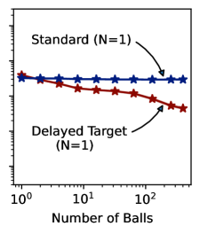
Figure 8: Ablation studies on the sampling hyper-parameters and settings. In the left plot, we compare the deterministic and i.i.d. sampling on the standard trainings with various $N$. In the middle plot, the horizontal axis shows the number of balls sampled in each epoch. Both the standard and the delayed target methods are shown in this plot with $N=1$. The right plot shows the training curves for the standard method with $N=1$ target samples. All experiments were conducted on the Poisson problem in Figure 1 of the main paper.

A.4 Ablation Studies

Here, we examine the effect of different design choices and hyper-parameters with different ablation studies. In particular, we focus on the 2D Poisson problem in Figure 1 of the main paper.

Surface point sampling scheme ablations:

Figure 8 compares the deterministic vs. i.i.d. sampling schemes and the effect of various mini-batch sizes (i.e., the number of volumes sampled in each epoch). The results suggest that the deterministic sampling scheme can train successfully with large $N$, however, it may not remedy the biased solution problem with the standard training at small $N$ values. Furthermore, the results indicate that the number of volumes in each epoch has minimal to no effect on the standard training method, which indicates that such a parallelization is not the bottleneck for the standard training method. To make this clear, we showed the training curves for the standard method, and they indicate similar trends and performance across a large range ($1$-$400$) of batch-size values for the standard method.

On the other hand, the performance of the delayed target method improves upon using a larger batch-size, which possibly indicates that this problem has a high objective estimation variance. The ability to trade large $N$ (i.e., high quality data) with a larger quantity is an advantage of the delayed target method relative to standard trainings.

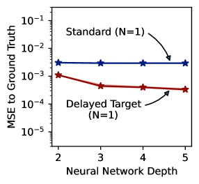
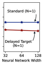
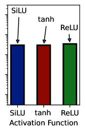
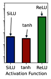
Figure 9: Ablating the function approximation class attributes on the 2D Poisson problem in Figure 1 of the main paper. A multi-layer perceptron was used in all of our experiments. The left and right line plots show the effect of the neural network’s depth and width, respectively, on each of the standard and delayed target methods. The left and right bar plots demonstrate the effect of the neural activation function on the standard and the delayed target methods, respectively. These results indicate that the function approximation class can have a more substantial impact on the delayed target method than the standard trainings.

Function approximation ablations:

Figure 9 compares the effect of the neural architecture parameters on the performance of the standard training vs. the delayed target method. All results are demonstrated on the 2D Poisson problem in Figure 1 of the main paper. The standard training exhibits a steady performance across all neural network depths, widths, and activation functions. However, the performance of the delayed target method seems to be enhancing with deeper and wider networks. The effect of the neural activation functions is more pronounced than the depth and width of the network. In particular, the ReLU activation performs substantially worse than the $\tanh$ or SiLU activations, and the $\tanh$ activation seems to yield the best results.

To shed some further light on the training behavior of the delayed target method, we show the training curves for different neural hyper-parameters in Figure 10. The results indicate that the ReLU activation prevents the delayed target method from improving during the entire training. On the other hand, the SiLU activation yields better initial improvements, but struggles to maintain this trend throughout the training. Based on this, we speculate that some activation functions (e.g., ReLU) may induce poor local optima in the optimization landscape of Algorithm 1, which may be difficult to run away from.

Our neural depth analysis in Figure 10 indicates that deeper networks can yield quicker improvements to the performance. However, such improvements are difficult to maintain stably over the entire course of training. In particular, the 2-layer training yields worse performance than the deeper networks, but maintains a monotonic improvement over the course of the training unlike the other methods. Of course, such behavior may be closely tied together with the activation function used for function approximation, as we discussed earlier.

We also show the effect of network width on the performance of the delayed target method in Figure 10. Wider networks are more likely to provide better initial improvements. However, as the networks are trained for longer, such a difference in performance shrinks, and narrower networks tend to show similar final performances as the wider networks.

All in all, our results indicate that the choice of the neural function approximation class, particularly with varying activation and depths, can have a notable impact on the performance of the delayed target method. We speculate that this is due to the incomplete gradients used during the optimization process of the delayed target method. The effect of incomplete function approximation on bootstrapping methods has been studied frequently, both in theory and practice, in other contexts such as the Fitted Q-Iteration (FQI) and Q-Learning methods within reinforcement learning. This is in contrast to the standard training methods, which seem quite robust to function approximation artifacts at the expense of solving an excess-variance diluted optimization problem.

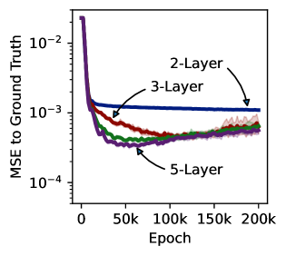
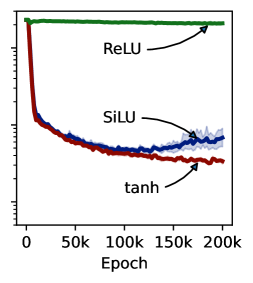
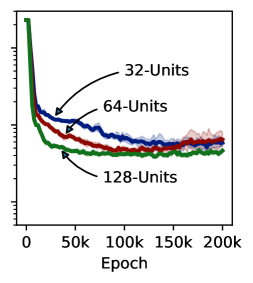
Figure 10: A closer look at the training curves for the delayed target method with different neural network hyper-parameters on the 2D Poisson problem in Figure 1 of the main paper. The left, middle, and right plots show the training curves for various neural depth, activation, and width, respectively.

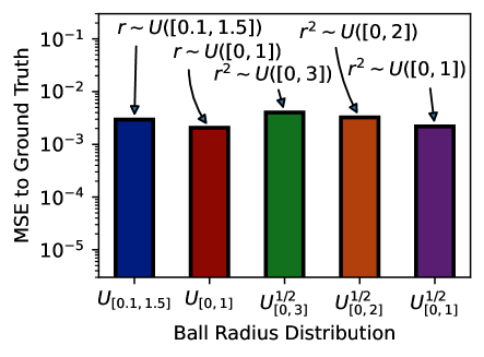
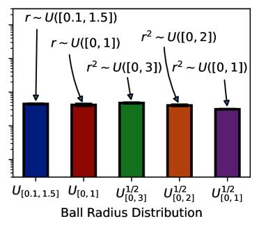
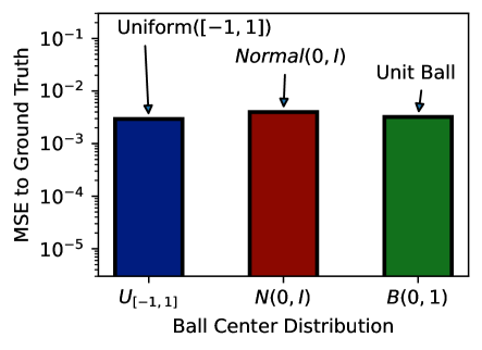
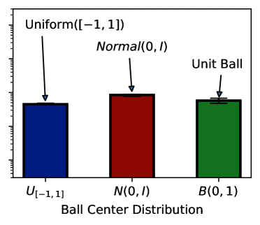
Figure 11: Ablating the distribution of ball centers and radii for both of the standard and the delayed target methods, both with $N=1$. The left column plots correspond to the standard method, and the the right column plots correspond to the delayed target method. The top row plots show the effect of the ball radius distribution, and the bottom row shows the effect of the ball center distribution. In the top row, $r\sim U([a,b])$ means the ball radius was sampled from a uniform distribution over $[a,b]$. Also, $r^{2}\sim U([a,b])$ means that the radius was the square root of a uniform random variable between $a$ and $b$. The ball centers were randomly picked either (1) uniformly over a square with the $[-1,-1],[-1,1],[1,1],[1,-1]$ vertices, (2) normally, or (3) uniformly within the unit ball.

Integration volume sampling ablations:

For our integration volumes, we randomly sampled balls of varying radii and centers. The distribution of the sampled radii and centers could impact the performance of different methods. Figure 11 studies such effects on both of the standard and the delayed target methods in the 2D Poisson problem of Figure 1 in the main paper. In short, we find that the delayed target method is robust to such sampling variations; an ideal method should find the same optimal solution with little regard to the integration volume distribution. On the other hand, our results indicate that the standard training performance tends to be sensitive to the integration volume distributions. This may be due to the fact that the standard trainings need to minimize two loss terms; the optimal balance between the desired loss function $\mathcal{L}_{\theta}(x)$ and the excess variance $\mathbb{V}_{P(x^{\prime}|x)}[g_{\theta}(x^{\prime})]$ in Equation (15) of the main paper may be sensitive to the distribution of $x$ itself.

Poisson charge placement ablations:

The charge locations in the 2D Poisson problem may impact the results for our methods. For this, we compare the standard and the delayed target method over a wide variety of charge distributions. Figure 12 summarizes these results. Here, the three fixed charge locations shown in Figure 1 of the main paper are shown as a baseline. We also show various problems where the charge locations were picked uniformly or normally in an i.i.d. manner. The performance trends seem to be quite consistent for each method, and the fixed charge locations seem to represent a wide range of such problems and datasets well.

Delayed target ablations:

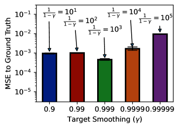
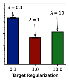
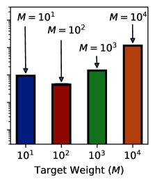
Figure 13: Ablating the effect of the delayed target method parameters on the 2D Poisson problem in Figure 1 of the main paper. The left plot shows the effect of the target smoothing parameter $\tau$ in Algorithm 1. The middle plot shows the effect of the target regularization parameter $\lambda$ in Algorithm 1. The right plot shows the effect of the target weight factor $M$ in Equation (23).

Three main hyper-parameters are involved in the definition of the delayed target method: (1) the target smoothing $\tau$, (2) the target regularization weight $\lambda$, and (3) the target weight $M$ described in Equation (23). Figure 13 studies the effect of each of these hyper-parameters on the performance of the delayed target method in the 2D Poisson problem in Figure 1 of the main paper.

Our results indicate that choosing a proper target smoothing can improve the performance of the delayed target method. In particular, neither a significantly small nor a substantially large $\tau$ can yield an optimal training. Small $\tau$ values cause the training target to evolve rapidly. This may accelerate the training initially, but it can negatively impact the final performance of the method as we show in Figure 13. On the other hand, too large values of $\tau$ can cause the target network to lag behind the main solution, thus bottlenecking the training. The optimal $\tau$ in this problem defines a smoothing window of size $1/(1-\gamma)=1000$, which seems relatively appropriate for a training duration of $200k$ epochs.

Next, we studied the effect of target regularization weight $\lambda$ in Algorithm 1. A small target weight causes this method to diverge in this particular problem, as we’ve shown in Figure 2 of the main paper. On the other hand, a regularization weight too large can slow down the training, as the main model remains too constrained to the target model during training.

We also show the effect of various target weight $M$ values in this problem. Ideally, $M\rightarrow\infty$ to make our approximations more accurate. A small target weight can effectively cause the method to seek biased solutions. On the other hand, setting $M$ too large may be impractical and instead cause the loss estimator’s variance to explode as discussed in Equation (23) of the main paper. For this, $M$ must be set in conjunction with the $\lambda$ hyper-parameter in such challenging problems.

A.5 Training Details

The Poisson Problem

To solve this system in the integrated form, the standard way of training PINNs is to fit a neural model with the following loss:

$$\hat{\mathcal{L}}=\mathbb{E}\bigg{[}\big{(}A_{d}^{r}\cdot\frac{1}{N}\sum_{i=1}^{N}E_{\theta}(x^{(i)})\cdot\hat{n}(x_{i})-y_{\Omega}\big{)}^{2}\bigg{]},$$ (34)

where $A_{d}^{r}:=\int_{\partial\Omega_{r}}1\text{ d}S$ is the surface area of a $d$-dimensional ball with the radius $r$, and the label is $y_{\Omega}=\iint_{\Omega}\nabla\cdot E\mathrm{d}V$.

The $x_{i}$ samples follow the $\text{Unif}\big{(}\partial\Omega_{r}\big{)}$ distribution. The sampling intensity for volume $\Omega$ defines the weight of the test constraints.

In this work, we consider a Poisson problem with $d=2$ dimensions and Dirac-delta charges. We place three unit charges at $[0,0]$, $[-0.5,-0.5]$, and $[0.5,0.5]$ coordinates. For this setup, computing $y_{\Omega}$ is as simple as summing the charges residing within the volume $\Omega$. The integration volumes are defined as random spheres. The center coordinates and the radius of the spheres are sampled uniformly in the $[-1,1]$ and $[0.1,1.5]$ intervals, respectively. We train all models for 200,000 epochs, where each epoch samples 1000 points in total. We also study higher-dimensional problems with $d\in[2,10]$ with a single charge at the origin.

Random effect matching

Random effects (random number generators seed; batch ordering; parameter initialization; and so on) complicate the study by creating variance in the measured statistics. We use a matching procedure (so that the baseline and the proposed models share the same values of all random effects) to control this variance. As long as one does not search for random effects that yield a desired outcome (we did not), this yields an unbiased estimate of the improvement. Each experiment is repeated 100 times to obtain confidence intervals. Note that (1) confidence intervals are small; and (2) experiments over many settings yield consistent results.

Poisson problem with singular charges

In this section, we examine solving a singular Poisson problem. In particular, we focus on learning the potentials for Dirac-delta charges. Of course, finding a strong solution by enforcing the Poisson equation directly may be impractical due to its sparsity and singularity. Therefore, we use the divergence theorem as a proxy for learning. This solution relies on estimating an integral over the volume surface, which may require many samples in high-dimensional spaces. Using few samples inside the MSE loss can induce an excess variance that would bias the solution towards overly smooth functions. Our first experiment in Figures 1, 2, and 3 define a 2-D Poisson problem with three unit Dirac-delta charges at $[0,0]$, $[-0.5,-0.5]$, and $[0.5,0.5]$. We also study higher-dimensional problems with a single charge at the origin in Figure 4.

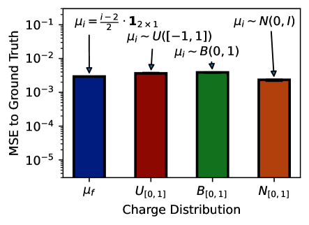
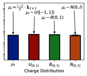
Figure 12: Ablating the location distribution of the three charges on the 2D Poisson problem in Figure 1 of the main paper. The left plot shows the results for the standard training method, while the the right plot corresponds to the delayed target method, all with $N=1$. The blue bar represents fixing the charge locations at the $[0,0]$, $[-0.5,-0.5]$, and $[0.5,0.5]$ coordinates. We also show the results for picking the charge locations in an i.i.d. manner (1) uniformly between $[-1,-1]$ and $[1,1]$ (denoted as $U([-1,1]$), (2) uniformly over the unit ball (denoted as $B(0,1)$), and (3) normally (denoted as $N(0,1)$).

The Maxwell problem with a rectangular current circuit

Our second example looks at finding the magnetic potentials and fields in a closed-circuit with a constant current. This defines a singular current density profile $J$. We consider a rectangular closed circuit in the 3-D space with the $[\frac{1}{\sqrt{3}},\frac{-1}{\sqrt{3}},\frac{-1}{\sqrt{3}}],[\frac{1}{\sqrt{3}},\frac{1}{\sqrt{3}},\frac{1}{\sqrt{3}}],[\frac{-1}{\sqrt{3}},\frac{1}{\sqrt{3}},\frac{1}{\sqrt{3}}]$, and $[\frac{-1}{\sqrt{3}},\frac{-1}{\sqrt{3}},\frac{-1}{\sqrt{3}}]$ vertices. The training volumes were defined as random circles, where the center coordinates and the surface normals were sampled from the unit ball, and the squared radii were sampled uniformly in the $[0.0,1.0]$ interval.

Smoluchowski coagulation problem

To simulate particle evolution dynamics, we consider a Smoluchowski coagulation problem where particles evolve from an initial density. We considered the particle sizes $x,x^{\prime}$ to be in the $[0,1]$ unit interval, and the simulation time to be in the $[0,1]$ unit interval as well. We designed the coagulation kernel $K(x,x^{\prime})$ to induce non-trivial solutions in our unit solution intervals. Specifically, we defined $K(x,x^{\prime})=1.23\times(\text{min}(1.14,\sqrt{x}+\sqrt{x^{\prime}}))^{3}$. To find a reference solution, we performed Euler integration using exact time-derivatives on a large grid size. The grid time-derivatives were computed by evaluating the full summations in the Smoluchowski coagulation equation.

Training hyper-parameters

We employ a 3-layer perceptron as our deep neural network, using 64 hidden neural units in each layer, and the Tanh activation function. We trained our networks using the Adam [12] variant of the stochastic gradient descent algorithm under a learning rate of $0.001$. For a fair comparison, we afforded each method 1000 point evaluations for each epoch. Table 3 provides a summary of hyper-parameters.

Hyper-Parameter	Value
Randomization Seeds	100
Learning Rate	0.001
Optimizer	Adam
Epoch Function Evaluations	1000
Training Epochs	200000
Network Depth	3
Network Width	64
Network Activation	SiLU

Hyper-Parameter	Value
Problem Dimensions	1, 2, and 3
Initial Condition Weight	1
Initial Condition Time	0
Initial Condition Points	Uniform([0,1])
Time Sampling Distribution	Uniform([0,1])
Particle Size Distribution	Uniform([0,1])
Ground Truth Integrator	Euler
Ground Truth Grid Size	10000

Hyper-Parameter	Value
Problem Dimension	2
Number of Poisson Charges	3
Integration Volumes	Balls
Volume Center Distribution	Uniform([-1,1])
Volume Radius Distribution	Uniform([0.1,1.5])

Hyper-Parameter	Value
Problem Dimension	3
Number of Wire Segments	4
Integration Volumes	2D Disks
Volume Center Distribution	Unit Ball
Volume Area Distribution	Uniform([0,1])

Table 3: A summary of the general and specific hyper-parameters in each problem. The top left table represents the common settings used in all experiments. The top right, bottom left, and bottom right tables correspond to the Smoluchowski, Poisson, and Maxwell problems, respectively.

A.6 Limitations

Our work solves the problem of learning from integral losses in physics informed networks. We mostly considered singular and high-variance problems for benchmarking our methods. However, problems with integral losses can have broader applications in solving systems with incomplete observations and limited dataset sizes. This was beyond the scope of our work. In fact, such applications may extend beyond the area of scientific learning and cover diverse applications within machine learning. We rigorously studied the utility of three methods for solving such systems. However, more algorithmic advances may be necessary to make the proposed methods robust and adaptive to the choice of the algorithmic and problem-defining hyper-parameters. The delayed target method was shown to be capable of solving challenging problems through its approximate dynamic programming nature. However, we did not provide a systematic approach for identifying its bottlenecks in case of a failed training. Understanding the pathology of the proposed methods is certainly a worthwhile future endeavor.

A.7 Broader Impact

This work provides foundational theoretical results and builds upon methods for training neural PDE solvers within the area of scientific learning. Scientific learning methods and neural PDE solvers can provide valuable models for a solving range of challenging applications in additive manufacturing [32, 20, 7], robotics [26], high speed flows [18], weather forecasting [17], finance systems [2] chemistry [10], computational biology [13], and heat transfer and thermodynamics [3].

Although many implications could result from the application of scientific learning, in this work we focused especially on settings where precision, singular inputs, and compatibility with partial observations are required for solving the PDEs. Our work particularly investigated methods for learning PDEs with integral forms, and provided effective solutions for solving them. Such improvements could help democratize the usage of physics informed networks in applications where independent observations are difficult or expensive to obtain, and the inter-sample relationships and constraints may contain the majority of the training information. Such problems may be challenging and the trained models are usually less precise than the traditional solvers. These errors can propagate to any downstream analysis and decision making processes and result in significant issues. Other negative consequences of this work could include weak interpretability of the trained models, increased costs for re-training the models given varying inputs, difficulty in estimating the performance of such trained models, and the existence of unforeseen artifacts in the trained models [29].

To mitigate the risks, we encourage further research to develop methods to provide guarantees and definitive answers about model behaviors. In other words, a general framework for making guaranteed statements about the behavior of the trained models is missing. Furthermore, more efficient methods for training such models on a large variety of inputs should be prioritized for research. Also, a better understanding the pathology of neural solvers is of paramount concern to use these models safely and effectively.

Our work consumed approximately 500 hours of training time on NVIDIA A50 GPUs.

References

- Arazo et al. [2020] Eric Arazo, Diego Ortego, Paul Albert, Noel E O’Connor, and Kevin McGuinness. Pseudo-labeling and confirmation bias in deep semi-supervised learning. In 2020 International Joint Conference on Neural Networks (IJCNN), pages 1–8. IEEE, 2020.
- Bai et al. [2022] Yuexing Bai, Temuer Chaolu, and Sudao Bilige. The application of improved physics-informed neural network (ipinn) method in finance. Nonlinear Dynamics, 107(4):3655–3667, 2022.
- Cai et al. [2021] Shengze Cai, Zhicheng Wang, Sifan Wang, Paris Perdikaris, and George Em Karniadakis. Physics-informed neural networks for heat transfer problems. Journal of Heat Transfer, 143(6), 2021.
- Chen et al. [2021] Yutian Chen, Liyuan Xu, Caglar Gulcehre, Tom Le Paine, Arthur Gretton, Nando de Freitas, and Arnaud Doucet. On instrumental variable regression for deep offline policy evaluation. arXiv preprint arXiv:2105.10148, 2021.
- Fujimoto et al. [2022] Scott Fujimoto, David Meger, Doina Precup, Ofir Nachum, and Shixiang Shane Gu. Why should i trust you, bellman? the bellman error is a poor replacement for value error. arXiv preprint arXiv:2201.12417, 2022.
- Ghaffari et al. [2022] Saba Ghaffari, Ehsan Saleh, David Forsyth, and Yu-Xiong Wang. On the importance of firth bias reduction in few-shot classification. In International Conference on Learning Representations, 2022. URL https://openreview.net/forum?id=DNRADop4ksB.
- Henkes et al. [2022] Alexander Henkes, Henning Wessels, and Rolf Mahnken. Physics informed neural networks for continuum micromechanics. Computer Methods in Applied Mechanics and Engineering, 393:114790, 2022.
- Hinton et al. [2015] Geoffrey Hinton, Oriol Vinyals, Jeff Dean, et al. Distilling the knowledge in a neural network. arXiv preprint arXiv:1503.02531, 2(7), 2015.
- Jagtap et al. [2020] Ameya D Jagtap, Ehsan Kharazmi, and George Em Karniadakis. Conservative physics-informed neural networks on discrete domains for conservation laws: Applications to forward and inverse problems. Computer Methods in Applied Mechanics and Engineering, 365:113028, 2020.
- Ji et al. [2021] Weiqi Ji, Weilun Qiu, Zhiyu Shi, Shaowu Pan, and Sili Deng. Stiff-pinn: Physics-informed neural network for stiff chemical kinetics. The Journal of Physical Chemistry A, 125(36):8098–8106, 2021.
- Kharazmi et al. [2021] Ehsan Kharazmi, Zhongqiang Zhang, and George Em Karniadakis. hp-vpinns: Variational physics-informed neural networks with domain decomposition. Computer Methods in Applied Mechanics and Engineering, 374:113547, 2021.
- Kingma and Ba [2014] Diederik P Kingma and Jimmy Ba. Adam: A method for stochastic optimization. arXiv preprint arXiv:1412.6980, 2014.
- Lagergren et al. [2020] John H Lagergren, John T Nardini, Ruth E Baker, Matthew J Simpson, and Kevin B Flores. Biologically-informed neural networks guide mechanistic modeling from sparse experimental data. PLoS computational biology, 16(12):e1008462, 2020.
- Lee et al. [2013] Dong-Hyun Lee et al. Pseudo-label: The simple and efficient semi-supervised learning method for deep neural networks. In Workshop on challenges in representation learning, ICML, volume 3, page 896, 2013.
- Li et al. [2019] Ke Li, Kejun Tang, Tianfan Wu, and Qifeng Liao. D3m: A deep domain decomposition method for partial differential equations. IEEE Access, 8:5283–5294, 2019.
- Li et al. [2020] Zongyi Li, Nikola Kovachki, Kamyar Azizzadenesheli, Burigede Liu, Kaushik Bhattacharya, Andrew Stuart, and Anima Anandkumar. Neural operator: Graph kernel network for partial differential equations. arXiv preprint arXiv:2003.03485, 2020.
- Mammedov et al. [2021] Yslam D Mammedov, Ezutah Udoncy Olugu, and Guleid A Farah. Weather forecasting based on data-driven and physics-informed reservoir computing models. Environmental Science and Pollution Research, pages 1–14, 2021.
- Mao et al. [2020] Zhiping Mao, Ameya D Jagtap, and George Em Karniadakis. Physics-informed neural networks for high-speed flows. Computer Methods in Applied Mechanics and Engineering, 360:112789, 2020.
- Mnih et al. [2015] Volodymyr Mnih, Koray Kavukcuoglu, David Silver, Andrei A Rusu, Joel Veness, Marc G Bellemare, Alex Graves, Martin Riedmiller, Andreas K Fidjeland, Georg Ostrovski, et al. Human-level control through deep reinforcement learning. nature, 518(7540):529–533, 2015.
- Niaki et al. [2021] Sina Amini Niaki, Ehsan Haghighat, Trevor Campbell, Anoush Poursartip, and Reza Vaziri. Physics-informed neural network for modelling the thermochemical curing process of composite-tool systems during manufacture. Computer Methods in Applied Mechanics and Engineering, 384:113959, 2021.
- NVIDIA [2022] NVIDIA. Physics informed neural networks in modulus, Apr 2022. URL https://docs.nvidia.com/deeplearning/modulus/text/theory/phys_informed.html.
- Pham et al. [2021] Hieu Pham, Zihang Dai, Qizhe Xie, and Quoc V Le. Meta pseudo labels. In Proceedings of the IEEE/CVF Conference on Computer Vision and Pattern Recognition, pages 11557–11568, 2021.
- Raissi et al. [2019] Maziar Raissi, Paris Perdikaris, and George E Karniadakis. Physics-informed neural networks: A deep learning framework for solving forward and inverse problems involving nonlinear partial differential equations. Journal of Computational physics, 378:686–707, 2019.
- Saleh and Jiang [2019] Ehsan Saleh and Nan Jiang. Deterministic bellman residual minimization. In Proceedings of Optimization Foundations for Reinforcement Learning Workshop at NeurIPS, 2019.
- Shukla et al. [2021] Khemraj Shukla, Ameya D Jagtap, and George Em Karniadakis. Parallel physics-informed neural networks via domain decomposition. Journal of Computational Physics, 447:110683, 2021.
- Sun et al. [2022] Wentao Sun, Nozomi Akashi, Yasuo Kuniyoshi, and Kohei Nakajima. Physics-informed recurrent neural networks for soft pneumatic actuators. IEEE Robotics and Automation Letters, 7(3):6862–6869, 2022.
- Sutton [1988] Richard S Sutton. Learning to predict by the methods of temporal differences. Machine learning, 3(1):9–44, 1988.
- Wang et al. [2022a] Justin L Wang, Jeffrey H Curtis, Nicole Riemer, and Matthew West. Learning coagulation processes with combinatorial neural networks. Journal of Advances in Modeling Earth Systems, page e2022MS003252, 2022a.
- Wang et al. [2021] Sifan Wang, Yujun Teng, and Paris Perdikaris. Understanding and mitigating gradient flow pathologies in physics-informed neural networks. SIAM Journal on Scientific Computing, 43(5):A3055–A3081, 2021.
- Wang et al. [2022b] Sifan Wang, Shyam Sankaran, and Paris Perdikaris. Respecting causality is all you need for training physics-informed neural networks. arXiv preprint arXiv:2203.07404, 2022b.
- Yin et al. [2022] Shuyu Yin, Tao Luo, Peilin Liu, and Zhi-Qin John Xu. An experimental comparison between temporal difference and residual gradient with neural network approximation. arXiv preprint arXiv:2205.12770, 2022.
- Zhu et al. [2021] Qiming Zhu, Zeliang Liu, and Jinhui Yan. Machine learning for metal additive manufacturing: predicting temperature and melt pool fluid dynamics using physics-informed neural networks. Computational Mechanics, 67:619–635, 2021.