Generalizing Parametrization Invariance in the Calculus of Variations

Abstract

We revisit the notion of parametrization invariance while introducing certain weakened notions of invariance in the calculus of variations. In this work, we employ a straightforward approach in the classical setting and mostly restrict attention to functionals on one-dimensional domains. We establish a connection between parametrization invariant functionals and functionals embodying a weaker notion of invariance of their Lagrangian; we term this notion as $\mathcal{T}$-Lagrangian analogous to the well-known idea of null Lagrangian. However, the Euler-Lagrange operator of a $\mathcal{T}$-Lagrangian vanishes only along the tangential direction in the configuration space. On one-dimensional domain and for first- and second-order theories, we show that functional described by such a Lagrangian is necessarily a parametrization invariant functional modulo null Lagrangian. Keeping the motivation for partial differential equations, we also introduce and explore the notion of $\mathcal{N}$-Lagrangian, with an invariance complementary to the case of $\mathcal{T}$-Lagrangian, whose Euler-Lagrange operator vanishes along normal directions. We find that in a one-dimensional setting, every $\mathcal{N}$-Lagrangian is simply a null Lagrangian.

Keywords: Parametric invariance, Null Lagrangian, Nilpotent energy, Helfrich-Canham energy, Minimal surfaces, Euler-Lagrange equations

Introduction

Parametrization invariance, often called parametric invariance and also sometimes called reparametrization invariance, is related to an important symmetry of many physical theories [GM21] due to their underlying geometric structure. For instance, it manifests in the theory of general relativity [TMW00] as a consequence of the principle of general covariance [Nor93] – that the equations of physics must be independent of the choice of coordinate systems. Most theories of quantum gravity, including string theory, therefore, inherit this symmetry [HS86].

In physics, parametrization invariance is also encountered as an important example of gauge symmetry [FGT99], a symmetry characterized by an infinite-dimensional Lie group of transformations of a functional (often referred as the action). The symmetry group for parametrization invariance is a diffeomorphism group. A defining feature of gauge theories (theories possessing gauge symmetry) is that their Euler-Lagrange equations are necessarily under-determined. This can be seen to arise as a consequence of Noether’s second theorem [Olv86, HM11]. In the case of parametrization invariant functionals, in fact, the component of the Euler-Lagrange operator in the tangential direction to the field variable is trivially zero.

Parametrization invariance is not limited to theories of high-energy physics; it also occurs with a firm footing in traditional continuum mechanics. For example, it is a defining symmetry of the Helfrich-Canham model (discussed in more detail in Sec. 1) [Can70, Hel73] for lipid bilayer membranes and of the theory of minimal surfaces (a model for soap films) [GH04] besides being an important geometric feature of the Euler elastica [Eul44]. It is evident that these theories are independent of the parametrization chosen to describe the surface. In the Helfrich-Canham model, parametrization invariance accounts for the in-plane fluidity of the lipid membrane [CG02]; the lipid molecules freely flow on the surface of the membrane, encountering very little resistance from the surrounding molecules. In this way, the parametrization invariance of the Helfrich-Canham energy can be ascribed to the lack of a well-defined in-plane reference configuration for the membrane. On the other hand, the parametrization invariance of the problem of Euler elastica arises solely out of the elastic property of the deformation where the stored energy per unit length in deformed configuration depends only on the current curvature. The equations of motion (Euler-Lagrange equations) for these theories are typically derived by taking variations of the surface or to the curve in the normal and tangential directions to the surface [CG02, CM11]. It can be shown [Ste+03] that the tangential component of the Euler-Lagrange operator is trivially zero.

Indeed, the equations of motion, or evolution equations, for several phenomena in physics and mechanics, including those alluded to in previous paragraph, are typically derived as Euler-Lagrange equations by taking variations of the field in the normal and tangential directions in configuration space considered to be embedded in a containing Euclidean space, wherein the starting point for the mathematical formulation is the proposal of an energy functional that satisfies certain symmetries (for example, the parametrization invariance for the examples noted above). In continuum mechanics, particularly in the theory of elastic media, such models are called hyperelastic models and are examples of conservative systems. However, in some cases, the theory for a physical system is formulated by starting with the equations of motion using balance laws such as balance of linear and angular momentum, mass, etc; one such example is Nagdhi’s formulation for shell theory [Nag73]. In such a class of physical models, where the analog of parametrization invariance is provided at the level of equations of motion, it is unclear which class of functionals fulfills that role in an exhaustive manner. It is also important to note that the way to analyze models with a restricted kind of fluid-invariance is speculative too; the latter is anticipated to be relevant with the inclusion of microscopic effects or environmental changes, c.f., chapter 10, [NPW04],[Des09].

At this point a question that naturally arises is — What is the analog of parametrization invariance of integrals/functionals at the level of differential equations of motion? In this paper, we explore this question by introducing a weakened notion of invariance of a Lagrangian which we term $\mathcal{T}$-Lagrangian. We address this issue in one dimension where we use elementary calculus to show that a weakened notion of invariance is interesting. We prove general representation result (Theorems 3.1 and 4.1) for the $\mathcal{T}$-Lagrangian and connect it to parametrization invariance. We also explore the complementary notion of an $\mathcal{N}$-Lagrangian. Surprisingly, we find that (Theorem 5.1) in the one-dimensional setting, $\mathcal{N}$-Lagrangians are exactly classical null Lagrangians [Ede62, Eri62, Run66]. We conjecture that generalizing these concepts to higher dimensions may offer nontrivial implications. It is also plausible that $\mathcal{N}$-Lagrangian may not be as trivial as it is in the one-dimensional case; it is worth a note that the characterization of null Lagrangians itself is a daunting task in higher dimensions and complex field theories, see [SB21] for a recent application of the results of [OS88]. Altogether these weakened notions of invariance are anticipated to involve a significant role played by null Lagrangians. Regarding the ways of the present paper, the simplicity of presented one-dimensional setting also allows a possible analysis on lines of [BCS16] that exploits jet bundle formalism; it is expected that the same formalism becomes handy and has strong potential in higher dimensions where our approach becomes tedious.

Overall, the intended plan in this paper concerns addressing the rephrased question: What are the functionals that satisfy the weakened notion of invariance with their Euler-Lagrange equations becoming trivial in certain directions (depending on the field), or, equivalently, remaining non-vanishing in certain directions (for some fields)? In this paper, we take only a first step towards posing this question and answering it in a simple setting while the future plan is attaining the ambitious goal of extending the introduced notions and concomitant analysis to partial differential equations.

This paper is organized as follows. In Sec. 1, we motivate our work using few examples of parametrization invariant functionals. In Sec. 2, we revisit the notion of parametrization invariance and briefly dwell upon a well-known property of parametrization invariant functionals. In Sec. 3, we introduce the notion of $\mathcal{T}$-Lagrangian and prove the representation theorem (Theorem 3.1) for such Lagrangians of first-order. The counterpart for second-order theories (Theorem 4.1) is discussed in Sec. 4. In Sec. 5, we introduce the notion of $\mathcal{N}$-Lagrangian and similarly derive a representation result but only for the case of first order. In Sec. 6 we discuss few more aspects of the analysis in the context of some continuum theories. We summarize our conclusions and point out a few related questions in Sec. 7.

1 Motivation

First we discuss some examples from continuum mechanics to motivate the notion of $\mathcal{T}$-Lagrangian. These examples serve as templates for first-order and second-order theories, respectively. As already referred in the introduction to this paper, we consider: theory of minimal surfaces, the Helfrich-Canham theory for fluid membranes, and the Euler elastica.

A minimal surface $\omega\subset\mathbb{R}^{3}$ is a minimizer of its total (surface) area functional [CM11]:

$$\mathcal{E}_{MS}=\int_{\omega}\;da,$$ (1)

subject to some prescribed boundary conditions. Here $da$ is the area measure on $\omega$. The classical Plateau’s problem concerns establishing the existence of such surfaces, which plays an important role in understanding the shape of soap films [AT76].

The second example we consider is the Helfrich-Canham theory [Can70, Hel73] for modeling the bending elasticity of lipid bilayer membranes. The energy functional for the corresponding model is given by

$$\mathcal{E}_{HC}=\int_{\omega}(\kappa H^{2}+\kappa_{g}K)\;da,$$ (2)

where $\omega$ is the surface describing the deformed membrane, $H$ is the mean curvature of the surface, $K$ is the Gaussian curvature, and $\kappa$ and $\kappa_{g}$ are the bending moduli. These functionals depend only on geometric entities associated with $\omega$, it is independent of the parametrization chosen to describe the surface. Indeed, parametrization invariance manifests to account for the in-plane fluidity of the lipid membranes [CG02]; the lipid molecules freely flow on the surface of the membrane, encountering very little resistance from the surrounding molecules. In this way, parametrization invariance of the Helfrich-Canham energy (2) can be ascribed to the lack of a well-defined in-plane reference configuration for the membrane.

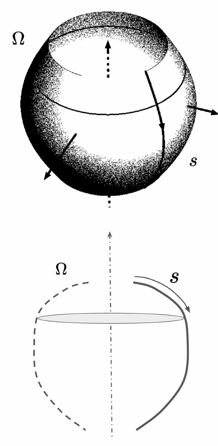
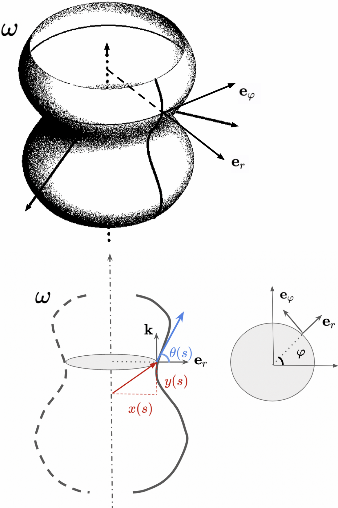
(a)	(b)

Figure 1: (a) Reference configuration for an axisymmetric surface $\Omega$ (b) Deformed configuration $\omega$, with the deformation map $\mathbf{f}(s,\varphi)=x(s)\mathbf{e}_{r}+y(s)\mathbf{k}$.

Since this paper focuses on one-dimensional domains, we specialize both above theories, i.e., involving (1) and (2), for the case of axisymmetric configurations. Let $\Omega$ represent an axisymmetric reference configuration of the surface whose associated arc length parameter is denoted as $s$ (shown schematically in Fig. 1a). The total arc length along the cross-section is $L$, thus $s\in[0,L]$. Let $\omega$ represent the deformed configuration and the deformation map (shown schematically in red in Fig. 1b) for the surface $\omega$ is parametrized as

$$\mathbf{f}(s,\varphi)=x(s)\mathbf{e}_{r}(\varphi)+y(s)\mathbf{k},\;s\in[0,L],$$ (3)

where $\mathbf{e}_{r}(\varphi)$, and $\mathbf{k}$ are the basis vectors in the cylindrical coordinates, with $\varphi$ denoting the azimuthal angle. The angle between the tangent to $\omega$ at $s$ and $\mathbf{e}_{r}$ is denoted as $\theta(s)$. It is clear that

$$\tan\theta(s)=\frac{y^{\prime}(s)}{x^{\prime}(s)},$$

where the prime denotes the derivative with respect to $s$. It can be shown that (to avoid clutter, omitting to write the explicit dependence on $s$)

$$da=x\sqrt{x^{\prime 2}+y^{\prime 2}}\;ds\;d\varphi,$$

$$H=\frac{1}{2}\Big{(}\frac{\theta^{\prime}}{\sqrt{x^{\prime 2}+y^{\prime 2}}}+\frac{\sin\theta}{x}\Big{)},\quad K=\frac{\theta^{\prime}\sin\theta}{x\sqrt{x^{\prime 2}+y^{\prime 2}}}.$$

With restriction to consider only axisymmetric configurations, the minimal surface energy (1) can be written as

$$\mathcal{E}_{MS}=2\pi\int_{0}^{L}x\sqrt{x^{\prime 2}+y^{\prime 2}}\;ds,$$ (4)

while the Helfrich-Canhman energy (2) can be written as

$$\begin{split}\mathcal{E}_{HC}&=2\pi\int_{0}^{L}\Bigg{(}\frac{\kappa}{4}\Big{(}\frac{\theta^{\prime}}{\sqrt{x^{\prime 2}+y^{\prime 2}}}+\frac{\sin\theta}{x}\Big{)}^{2}\\ &\qquad+\kappa_{g}\frac{\theta^{\prime}}{\sqrt{x^{\prime 2}+y^{\prime 2}}}\frac{\sin\theta}{x}\Bigg{)}x\sqrt{x^{\prime 2}+y^{\prime 2}}\;ds.\end{split}$$ (5)

By inspection it is clear that (4) is a first-order theory since the highest derivative appearing in the functional is of first-order, while (5) is a second-order theory where the functional depends on $\theta^{\prime}=(x^{\prime}y^{\prime\prime}-y^{\prime}x^{\prime\prime})/(x^{\prime 2}+y^{\prime 2})$ (see LABEL:appx:sec:axisymm_formulation of supplementary for details).

As another example of second-order theory, which is inherently one-dimensional, we consider the Euler Elastica [Eul44]. In this classic example (chapter 19, [Lov27]), a rod (of reference length $L$) is described as a curve in two dimensions with its deformation map parametrized as

$$\mathbf{r}(s):=x(s)\mathbf{i}+y(s)\mathbf{j},$$ (6)

where $s$ is a parametrization of the reference arc-length of the rod. The energy density (in the deformed configuration) for an Euler elastica is proportional to the square of the curvature, the latter explicitly given by $\kappa(s)=(x^{\prime}y^{\prime\prime}-y^{\prime}x^{\prime\prime})/(x^{\prime 2}+y^{\prime 2})^{3/2}$. Thus the total energy is given by

$$\mathcal{E}_{e}=\int_{0}^{L}\Big{(}\frac{x^{\prime}y^{\prime\prime}-y^{\prime}x^{\prime\prime}}{(x^{\prime 2}+y^{\prime 2})^{3/2}}\Big{)}^{2}\;\sqrt{x^{\prime 2}+y^{\prime 2}}\;ds.$$ (7)

Indeed, (7) belongs to the class of second-order theories.

As mentioned before, these three examples serve as templates for the discussion below where we follow a pedestrian approach, mostly employing freshman calculus, in the classical framework of the calculus of varitions [GFS00] and restrict attention to functionals on one-dimensional domains. We remark that, in addition to the surface of revolution described above, the extruded surfaces, obtained from a curve, can also be considered (where $K=0$) leading to another class of simple one dimensional problems but we omit the details for these as they appear to be less interesting from viewpoint of applications we have discussed so far.

Notation

Following the standard notation in mathematics and mechanics [Gur82], the set of real numbers is denoted by $\mathbb{R}$ whereas the $n$ dimensional real linear space (with $n$-tuplets) is denoted by $\mathbb{R}^{n}$, which is further equipped with the standard inner-product which we denote with a dot, i.e., $\mathbf{a}\cdot\mathbf{b}$. The standard basis of $\mathbb{R}^{n}$ is denoted by $\{\mathbf{e}_{i}\}_{i=1}^{n}.$ We use boldface font to represent the vectors and tensors. The inherited standard basis for second order tensors is $\{\mathbf{e}_{i}\otimes\mathbf{e}_{j}\}_{i,j=1}^{n}$ with the second order tensor $\mathbf{a}\otimes\mathbf{b}$, for given $\mathbf{a},\mathbf{b}\in\mathbb{R}^{n}$, defined as a linear transformation from $\mathbb{R}^{n}$ to $\mathbb{R}^{n}$ such that $(\mathbf{a}\otimes\mathbf{b})[\mathbf{x}]=\mathbf{a}(\mathbf{x}\cdot\mathbf{b})$ for all $\mathbf{x}\in\mathbb{R}^{n}$; the square brackets denote the linear action of an operator, which is mostly clear from the context. We also employ the usual summation convention when the indicial notation is unambiguous to describe tensorial manipulations, for example $\mathbf{a}=a_{i}\mathbf{e}_{i},\mathbf{A}[\mathbf{x}]=\mathbf{A}\mathbf{x}=A_{ij}x_{j}\mathbf{e}_{i},\mathbf{a}\cdot\mathbf{b}=a_{i}b_{i},$ etc for vectors $\mathbf{a},\mathbf{b},\mathbf{x}$ and second order tensor $\mathbf{A}$; otherwise, we stick to explicit sums. In particular $\mathbf{a}\otimes\mathbf{b}=a_{i}b_{j}\mathbf{e}_{i}\otimes\mathbf{e}_{j}.$ We define the transpose of a tensor in a way that $(\mathbf{a}\otimes\mathbf{b})^{T}=a_{j}b_{i}\mathbf{e}_{i}\otimes\mathbf{e}_{j}.$ $D_{s}$ represents the total derivative with respect to $s$ treating all arguments as functions of $s$. $D_{1},D_{2},\dotsc$ represents the (partial) derivative with respect to $1$st argument, $2$nd argument. For brevity and emphasis, we sometimes abuse the notation and alternate between a comma notation and an explicit form, i.e., $f_{,x}(x,y)=\partial_{x}f(x,y)=\frac{\partial}{\partial x}f(x,y)$, $f_{,xy}=\partial_{xy}f(x,y)=\frac{\partial^{2}}{\partial y\partial x}f(x,y)$, etc. We use square brackets to represent a linear operator’s action with an exception of the similar notation for a closed interval of the real line. The unit sphere in $n$-dimensions is $\mathcal{S}^{n-1},$ while the corresponding torus $\mathcal{S}^{1}\times\dotsc\times\mathcal{S}^{1}$ is denoted by $(\mathcal{S}^{1})^{n-1}$.

In the rest of this paper, we only consider functionals on one-dimensional domains, which we set to $[0,1]$ without any loss of generality. We assume that the Lagrangian $\mathscr{L}$ is, in general, a smooth function of $s\in[0,1]$, an $n$-dimensional field

$${{\mathbf{u}}(s):=u_{i}(s)\mathbf{e}_{i}\in\mathbb{R}^{n},}$$ (8)

i.e., simply the $n$-tuplet $(u_{1}(s),u_{2}(s),\dotsc,u_{n}(s))$, and its first and second derivatives, ${\mathbf{u}}{{}^{\prime}}(s)$ and ${\mathbf{u}}^{\prime\prime}(s)$. The energy functional with Lagrangian $\mathscr{L}$ is given by

$$\mathcal{E}({\mathbf{u}})=\int_{0}^{1}\mathscr{L}(s,{\mathbf{u}}(s),{\mathbf{u}}^{\prime}(s),{\mathbf{u}}^{\prime\prime}(s))\;ds.$$ (9)

If $\mathscr{L}$ explicitly depends on ${\mathbf{u}}^{\prime\prime}$, we call it a second-order Lagrangian. We assume that $n>1$ and denote the Euler-Lagrange operator acting on ${\mathbf{u}}$ as

$$\mathfrak{E}_{\mathscr{L}}({\mathbf{u}}):=\mathscr{L}_{\mathbf{u}}-D_{s}\mathscr{L}_{{\mathbf{u}}^{\prime}}+D_{ss}\mathscr{L}_{{\mathbf{u}}^{\prime\prime}},$$ (10a)

where

$$\begin{split}\mathscr{L}_{{\mathbf{u}}}&:=\mathscr{L}_{,z_{i}}(s,\mathbf{z},\mathbf{p},\mathbf{q})|_{\mathbf{z}={\mathbf{u}}(s),\mathbf{p}={\mathbf{u}}^{\prime}(s),\mathbf{q}={\mathbf{u}}^{\prime\prime}(s)}\mathbf{e}_{i},\\ \mathscr{L}_{{\mathbf{u}}^{\prime}}&:=\mathscr{L}_{,p_{i}}(s,\mathbf{z},\mathbf{p},\mathbf{q})|_{\mathbf{z}={\mathbf{u}}(s),\mathbf{p}={\mathbf{u}}^{\prime}(s),\mathbf{q}={\mathbf{u}}^{\prime\prime}(s)}\mathbf{e}_{i},\\ \mathscr{L}_{{\mathbf{u}}^{\prime\prime}}&:=\mathscr{L}_{,q_{i}}(s,\mathbf{z},\mathbf{p},\mathbf{q})|_{\mathbf{z}={\mathbf{u}}(s),\mathbf{p}={\mathbf{u}}^{\prime}(s),\mathbf{q}={\mathbf{u}}^{\prime\prime}(s)}\mathbf{e}_{i}.\end{split}$$ (10b)

The first variation [GFS00] of (9) with respect to smooth perturbations $\delta{\mathbf{u}}$ of ${\mathbf{u}}$ is denoted as $\delta\mathcal{E}[\delta{\mathbf{u}}]$, a linear functional of $\delta{\mathbf{u}}$. That is,

$$\delta\mathcal{E}[\delta{\mathbf{u}}]=\int_{0}^{1}(\mathscr{L}_{{\mathbf{u}}}\cdot\delta{\mathbf{u}}+\mathscr{L}_{{\mathbf{u}}^{\prime}}\cdot\delta{\mathbf{u}}^{\prime}+\mathscr{L}_{{\mathbf{u}}^{\prime\prime}}\cdot\delta{\mathbf{u}}^{\prime\prime})\;ds,$$ (11)

where the dot represents the Euclidean inner product in $\mathbb{R}^{n}$.

Let us introduce the notation

$$\mathcal{C}^{m}:=C^{m}([0,1];\mathbb{R}^{n}$$ (12)

We assume that ${\mathbf{u}}\in\mathcal{C}^{4}$ for any non-negative integer $m$) and the perturbations

$$\delta{\mathbf{u}}\in\mathcal{C}^{\infty}_{c}:=C^{\infty}_{c}([0,1];\mathbb{R}^{n}).$$ (13)

As is conventional in geometry and analysis, we use the word ‘curve’ to describe a one-dimensional manifold in $\mathbb{R}^{n}$ where $n$ is a positive integer; we use $n=2$ for illustration of some results. The function space

$$\mathcal{C}^{m}_{R}:=\{{\mathbf{u}}\in\mathcal{C}^{m}:\text{the curve }{\mathbf{u}}([0,1])\subset\mathbb{R}^{n}\text{ admits regular parametrization}\}$$ (14)

is used frequently in the paper. Notice that $\mathcal{C}^{m}_{R}$ is not a subspace of $\mathcal{C}^{m}$ but it can be considered as a candidate function space for variational analysis as $\mathcal{C}_{c}^{\infty}$ variations do not alter regularity mentioned in (14).

In the context of the statements and discussion in the following, specially using (9) and (11), we emphasize that whenever $\mathscr{L}$ is independent of ${\mathbf{u}}^{\prime\prime}$, we call such it a first-order Lagrangian; Naturally, in this case, it is sufficient to assume that ${\mathbf{u}}\in\mathcal{C}^{2}$.

2 Revisiting parametrization invariance

The purpose of this section is to recall an important consequence of parametrization invariance. The reader may note that we do not claim any originality in this section but provide these details as a simple recall of certain elementary facts.

We consider a diffeomorphism $\varpi:[0,1]\to[0,1]$ satisfying $\varpi(0)=0$ and $\varpi(1)=1$. As a parametrization of the curve defined by ${\mathbf{u}}$, we use $t=\varpi^{-1}(s)$ as the symbol for a new parameter in place of $s$ for given ${\mathbf{u}}\in\mathcal{C}^{4}_{R}$; thus, $s=\varpi(t)$ such that $\varpi(0)=0,\varpi(1)=1$.

Definition 2.1 [Parametrization Invariance].

$\mathcal{E}$ is said to be parametrization invariant if for any ${\mathbf{u}}\in\mathcal{C}_{R}^{4}$

$$\mathcal{E}({\mathbf{u}}\circ\varpi)=\mathcal{E}({\mathbf{u}}),$$ (15)

for any parametrization $\varpi$.

As a consequence of this symmetry, the tangential component of the Euler-Lagrange operator vanishes trivially. This is stated formally by

Proposition 2.1 .

If the functional (9) is parametrization invariant, then for any ${\mathbf{u}}\in\mathcal{C}^{4}_{R}$,

$$\mathfrak{E}_{\mathscr{L}}({\mathbf{u}})\cdot{\mathbf{u}}^{\prime}\equiv 0,$$ (16)

that is, $(\mathscr{L}_{\mathbf{u}}-D_{s}\mathscr{L}_{{\mathbf{u}}^{\prime}}+D_{ss}\mathscr{L}_{{\mathbf{u}}^{\prime\prime}})\cdot\mathbf{u}^{\prime}\equiv 0$.

This result is a special case of Noether’s second theorem [Olv86], and a proof of this result is included in the supplementary material. For first-order Lagrangians, in the above proposition, naturally it sufficient to assume that ${\mathbf{u}}\in\mathcal{C}^{2}_{R}$.

Indeed, the (integral or global) condition of parametrization invariance constrains a first-order Lagrangian to take a special form. For the convenience of the reader, we present a classical, and an elementary, argument [GH04] for the more general $n$-dimensional case. Due to (15), we have the equations:

$$\int_{s_{1}}^{s_{2}}{\mathscr{L}}(s,{\mathbf{u}}(s),{\mathbf{u}}^{\prime}(s))\;ds =\int_{\varpi^{-1}(s_{1})}^{\varpi^{-1}(s_{2})}{\mathscr{L}}\Big{(}\varpi(t),{\mathbf{u}}\circ\varpi(t),({\mathbf{u}}\circ\varpi){{}^{\prime}}(t)/\varpi^{\prime}(t)\Big{)}\varpi^{\prime}(t)\;dt$$

$$=\int_{\varpi^{-1}(s_{1})}^{\varpi^{-1}(s_{2})}{\mathscr{L}}\Big{(}t,{\mathbf{u}}\circ\varpi(t),({\mathbf{u}}\circ\varpi)^{\prime}(t))\Big{)}\;dt,$$ (17)

with $(s_{1},s_{2})\subset[0,1].$ The first equality in (17) arises due to a change of variable of integration, while the second equation is a statement of invariance. Using the arbitrariness of $s_{1},s_{2}$, the condition equivalent to parametrization invariance is found to be

$${\mathscr{L}}\Big{(}\varpi(t),{\mathbf{u}}\circ\varpi(t),({\mathbf{u}}\circ\varpi){{}^{\prime}}(t)/\varpi^{\prime}(t)\Big{)}\varpi^{\prime}(t)={\mathscr{L}}(t,{\mathbf{u}}\circ\varpi(t),({\mathbf{u}}\circ\varpi)^{\prime}(t)))$$

for each $t\in(0,1)$. It is well known [GH04] that the following two conditions: (1) ${\mathscr{L}}$ is independent of $s$ and (2) ${\mathscr{L}}$ is a homogeneous function of degree one in ${\mathbf{u}}^{\prime}(t)$, are necessary and sufficient for the integral form of parametrization invariance as stated in Definition 2.1. We formalize this observation as

Theorem 2.1 .

A functional $\mathcal{E}$ with a first-order Lagrangian is parametrization invariant according to Definition 2.1 if and only if the Lagrangian ${\mathscr{L}}$ is independent of the parameter $s$ and ${\mathscr{L}}$ is a homogeneous function of degree one in ${\mathbf{u}}^{\prime}$.

As a counterpart of above statement for a second-order Lagrangian [BCS16] (for example, see Theorem A.31 and Remark A.32), we have

Theorem 2.2 .

A functional $\mathcal{E}$ with a second-order Lagrangian is parametrization invariant if and only if

$${\mathbf{u}}^{\prime}\cdot\mathscr{L}_{{\mathbf{u}}^{\prime\prime}} = 0,$$ (18a)

$${\mathbf{u}}^{\prime}\cdot(\mathscr{L}_{{\mathbf{u}}^{\prime}}-\frac{d}{ds}\mathscr{L}_{{\mathbf{u}}^{\prime\prime}})+{\mathbf{u}}^{\prime\prime}\cdot\mathscr{L}_{{\mathbf{u}}^{\prime\prime}}-\mathscr{L} = 0.$$ (18b)

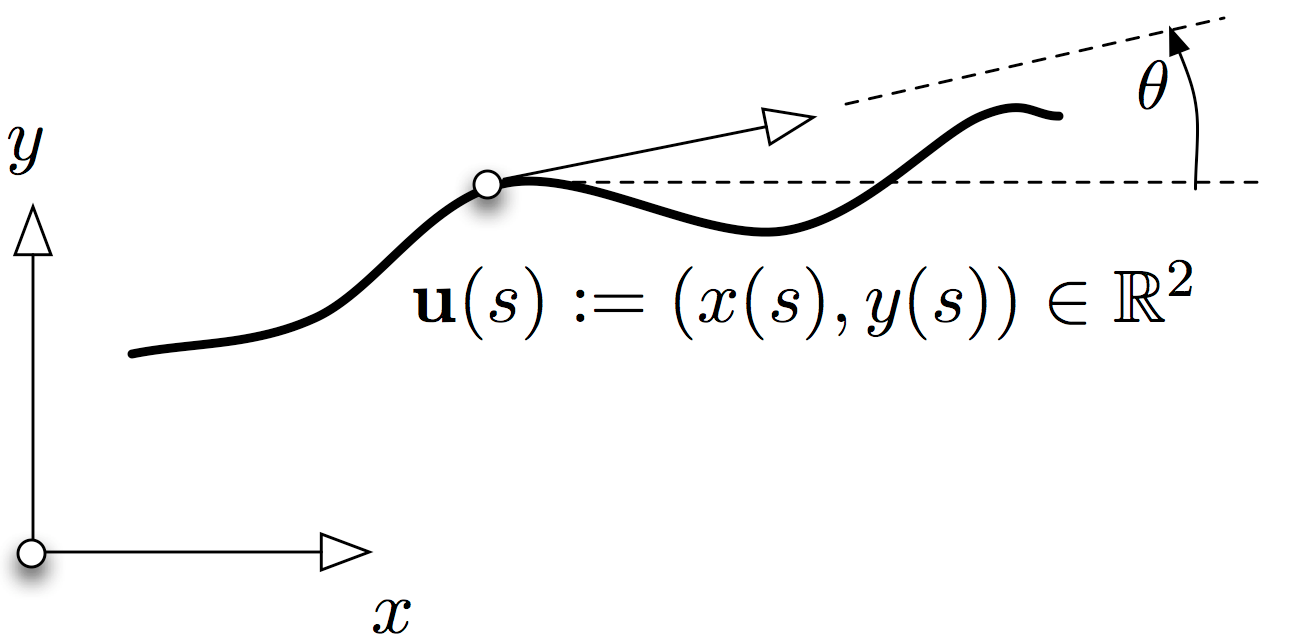
Figure 2: Schematic of the angle $\theta$ in $\mathbb{R}^{2}$.

Remark 2.1 .

In the case of $n=2$, i.e., when ${\mathbf{u}}([0,1])=\{(x(s),y(s)):s\in[0,1]\}\subset\mathbb{R}^{2}$ it can be shown for first order case that [GH04]

$$\mathscr{L}(s,(x(s),y(s)),(x^{\prime}(s),y^{\prime}(s)))=f\Big{(}x(s),y(s),\theta(s)\Big{)}\sqrt{x^{\prime}(s)^{2}+y^{\prime}(s)^{2}}$$ (19)

for some smooth function $f$, where $\theta(s)=\arctan(y^{\prime}(s)/x^{\prime}(s))$ can be interpreted as the tangent angle to the curve and $s\in[0,1]$; see Fig. 2 (c.f., Fig. 1b). This result is a consequence of Euler’s theorem for homogeneous functions. Similarly, for the two-dimensional (i.e., ${\mathbf{u}}(s)=(x(s),y(s))$) problem with a second-order Lagrangian [GH04], the Theorem 18 translates into the statement: A functional $\mathcal{E}$ with a second-order Lagrangian is parametrization invariant if and only if the Lagrangian has the form:

$$\begin{split}&\mathscr{L}{(s,(x(s),y(s)),(x^{\prime}(s),y^{\prime}(s)),(x^{\prime\prime}(s),y^{\prime\prime}(s)))}\\ &=g\Big{(}x(s),y(s),\theta(s),\theta^{\prime}(s)/\sqrt{x^{\prime}(s)^{2}+y^{\prime}(s)^{2}}\Big{)}\sqrt{x^{\prime}(s)^{2}+y^{\prime}(s)^{2}},\end{split}$$ (20)

where $g$ is an arbitrary (smooth) function and $\theta(s)=\arctan(y^{\prime}/x^{\prime})$. We retain the presence of $s$ on the left hand side of (19) and (20) for emphasis. At this point, it is appropriate to compare the structure of (19) with that of (4), and (20) with that of (5).

In summary, we see in Proposition 16 that the natural integral form of parametrization invariance implies a form of differential condition that the tangential component of the Euler-Lagrange operator vanishes. Parametrization invariance also restricts the form of the Lagrangian (c.f., Theorems 2.1 and 18). In this work, we explore a connection, in a sort of opposite implication, between Proposition 16 and Theorems 2.1 and 18, i.e. without the hypothesis of parametrization invariance.

3 $\mathcal{T}$- Lagrangian: case of tangential variations for first-order Lagrangians

The concept of $\mathcal{T}$-Lagrangian that we discuss below is motivated by relaxing the notion of parametrization invariance. Instead of requiring a global (integral) criterion, the invariance condition (15), we enforce a weaker, local (differential) condition of $\mathcal{T}$-Lagrangian, that we precisely state below.

If ${\mathbf{u}}\in\mathcal{C}^{2}_{R}$ (recall (14)), we define variations that are tangential and normal to the curve; note that ${\mathbf{u}}^{\prime}$ is non-vanishing. That is,

Definition 3.1 [Normal and Tangential variations].

Assume $n>1.$ Given a ${\mathbf{u}}\in\mathcal{C}_{R}^{2}$ the set

$$N_{\mathbf{u}}:=\{\mathbf{v}\in\mathcal{C}^{\infty}_{c}:{\mathbf{v}\cdot\mathbf{u^{\prime}}=0}\}$$

is the set of normal variations and

$$T_{\mathbf{u}}:=N_{\mathbf{u}}^{\perp}=\{\mathbf{v}\in\mathcal{C}^{\infty}_{c}:{\mathbf{v}=\psi\mathbf{u^{\prime}},\text{for some }\psi\in\mathcal{C}^{\infty}_{c}}\},$$

is the set of tangential variations.

Clearly, the direct sum $T_{\mathbf{u}}\oplus N_{\mathbf{u}}$ coincides with $\mathcal{C}^{\infty}_{c}$. Thus, $T_{\mathbf{u}}$ contains functions that have components tangential to ${\mathbf{u}}$, and $N_{\mathbf{u}}$ contains functions with components normal to ${\mathbf{u}}$.

Let us consider the following condition, motivated by (16), stated as

Definition 3.2 [$\mathcal{T}$-Lagrangian].

${\mathscr{L}}$ is a $\mathcal{T}$-Lagrangian if for every ${\mathbf{u}}\in\mathcal{C}_{R}^{2}$, $\delta\mathcal{E}[\delta{\mathbf{u}}]=0$ for all $\delta{\mathbf{u}}\in T_{\mathbf{u}}$.

That is, functional with a $\mathcal{T}$-Lagrangian necessitates that its first variation is trivially zero with respect to variations in a direction tangential to the curve ${\mathbf{u}}$. This definition contrasts with that of a classical null Lagrangian [Run66] whose first variation is trivially zero for all variations $\delta{\mathbf{u}}(s)$. Thus, $\mathcal{T}$-Lagrangian can be interpreted as a weakened notion of the classical null Lagrangian; recall that the Euler-Lagrange operator for a null Lagrangian is trivial. We show that an equivalent condition to check for the defining property of a $\mathcal{T}$-Lagrangian is a natural condition that the tangential component of the Euler-Lagrange operator is trivially zero.

Proposition 3.1 .

${\mathscr{L}}(s,{\mathbf{u}},{\mathbf{u}}^{\prime})$ is a $\mathcal{T}$-Lagrangian if and only if the tangential component of the Euler-Lagrange operator vanishes for all ${\mathbf{u}}\in\mathcal{C}^{2}_{R}$. That is,

$${\mathbf{u}}^{\prime}\cdot\mathfrak{E}_{\mathscr{L}}({\mathbf{u}})={\mathbf{u}}^{\prime}\cdot(-D_{s}{{\mathscr{L}}}_{{\mathbf{u}}^{\prime}}+{{\mathscr{L}}}_{\mathbf{u}})\equiv 0.$$ (21)

Proof

We first prove the forward implication, i.e., if $$\mathscr{L} \mathcal{T} {\mathbf{u}}\in\mathcal{C}^{2}_{R} \delta{\mathbf{u}}\in T_{\mathbf{u}}$$ is a -Lagrangian then (21) holds. For any given , let us consider variations . The first variation is given by

$$\delta\mathcal{E}[\delta{\mathbf{u}}]=\int_{0}^{1}\big{(}{{\mathscr{L}}}_{{\mathbf{u}}}\cdot\delta{\mathbf{u}}+{{\mathscr{L}}}_{{\mathbf{u}}^{\prime}}\cdot\delta{\mathbf{u}}^{\prime}\big{)}ds.$$ (22a)

which after integrating by parts yields

$$\delta\mathcal{E}[\delta{\mathbf{u}}]=\int_{0}^{1}\Big{(}\mathscr{L}_{\mathbf{u}}-D_{s}\mathscr{L}_{{\mathbf{u}}^{\prime}}\Big{)}\cdot\delta{\mathbf{u}}\;ds=0.$$ (22b)

Since $$\delta{\mathbf{u}}\in T_{\mathbf{u}} \delta{\mathbf{u}}=\psi(s){\mathbf{u}}^{\prime} \psi\in C_{c}^{\infty}[0,1]$$ it has the form , where . Therefore,

$$\delta\mathcal{E}[\delta{\mathbf{u}}]=\int_{0}^{1}\Big{(}\mathscr{L}_{\mathbf{u}}-D_{s}\mathscr{L}_{{\mathbf{u}}^{\prime}}\Big{)}\cdot{\psi{\mathbf{u}}^{\prime}}\;ds=0.$$

Since $\psi(s)$ is arbitrary, we obtain

$${\mathbf{u}}^{\prime}\cdot\Big{(}\mathscr{L}_{\mathbf{u}}-D_{s}\mathscr{L}_{{\mathbf{u}}^{\prime}}\Big{)}=0.$$ (22c)

The converse follows from the fact that if (21) holds, then the integrand in (22b) must be zero, whence $\delta\mathcal{E}[\delta{\mathbf{u}}]=0$ for all admissible variations. ∎

Just as in the case of parametrization invariant functionals, the tangential component of the Euler-Lagrange operator of a $\mathcal{T}$-Lagrangian is, thus, trivially zero. But for the latter, the converse also holds. In short, the vanishing of the tangential component is an equivalent local criterion for a Lagrangian to be a $\mathcal{T}$-Lagrangian.

3.1 Representation theorem for first-order $\mathcal{T}$- Lagrangian

Recall that Theorem 2.1 and Theorem 18 characterize the form of parametrization invariant Lagrangians. In this section, we derive the representation theorem for $\mathcal{T}$-Lagrangians. We focus on first-order Lagrangians in this section, while we consider the second-order case in the next.

In the proof of the representation theorem, a crucial role is played by

Lemma 3.1 .

If ${\mathscr{L}}(s,{\mathbf{u}},{\mathbf{u}}^{\prime})$ is a $\mathcal{T}$-Lagrangian then ${\mathscr{L}}$ has the form

$${\mathscr{L}}(s,{\mathbf{u}},{\mathbf{u}}^{\prime})={\mathbf{u}}^{\prime}\cdot{\mathbf{A}}(s,{\mathbf{u}},{\bm{\theta}})+C(s,{\mathbf{u}}),$$ (23a)

where $$C {\mathbf{A}}:=A_{i}\mathbf{e}_{i} A_{i} (i=1,\dotsc,n) s,{\mathbf{u}} {\bm{\theta}}\in(\mathcal{S}^{1})^{n-1}$$ is an arbitrary function (of variables indicated), , with as functions of , and , such that

$${\mathbf{A}}^{T}_{{\bm{\theta}}}(s,{\mathbf{u}},{\bm{\theta}})[{\mathbf{u}}^{\prime}]=\mathbf{0};\text{ for all }{\mathbf{u}}\in\mathcal{C}^{2}_{R},$$ (23b)

where $$\mathbf{A}_{{\bm{\theta}}}=\frac{\partial A_{i}}{\partial\theta_{j}}\mathbf{e}_{i}\otimes\mathbf{e}_{j} {\bm{\theta}}=(\theta_{1},\theta_{2},\dotsc,\theta_{n-1}) \hat{\mathbf{p}}={\mathbf{u}}^{\prime}/\left\lVert{\mathbf{u}}^{\prime}\right\rVert\in\mathcal{S}^{n-1}$$, and is associated with in the following manner (schematically shown in Fig. 3):

$$\begin{array}[]{l}\hat{p}_{1}=\cos\theta_{1},\\ \hat{p}_{2}=\sin\theta_{1}\cos\theta_{2},\\ \hat{p}_{3}=\sin\theta_{1}\sin\theta_{2}\cos\theta_{3},\\ \vdots\\ \hat{p}_{n-1}=\sin\theta_{1}\sin\theta_{2}\sin\theta_{3}\dotsc\sin\theta_{n-2}\cos\theta_{n-1},\\ \hat{p}_{n}=\sin\theta_{1}\sin\theta_{2}\sin\theta_{3}\dotsc\sin\theta_{n-2}\sin\theta_{n-1}.\end{array}$$ (23c)

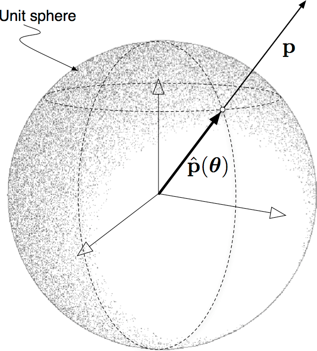
Figure 3: Schematic of ${\hat{\mathbf{p}}}({\bm{\theta}})$ in the polar coordinates $\mathbf{p}=\mathbf{p}(r,{\bm{\theta}})=r{\hat{\mathbf{p}}}({\bm{\theta}})$ in $\mathbb{R}^{n}$.

Proof

Since $${\mathscr{L}}(s,{\mathbf{u}},{\mathbf{u}}^{\prime}) \mathcal{T} {\mathbf{u}}\in\mathcal{C}^{2}_{R}$$ is a - Lagrangian, we have (from Proposition 21) for any ,

$$(-D_{s}({{\mathscr{L}}}_{{\mathbf{u}}^{\prime}})+{{\mathscr{L}}}_{\mathbf{u}})\cdot{\mathbf{u}}^{\prime}=0.$$

Let us define

$$\mathbf{p}:={\mathbf{u}}^{\prime},$$

i.e., we consider $${\mathscr{L}}(s,{\mathbf{u}},\mathbf{p})$$. Recall the definitions (or consider their natural analogues) (10b), i.e.

$${\mathscr{L}}_{\mathbf{p}}:={\mathscr{L}}_{,p_{i}}\mathbf{e}_{i},\quad{\mathscr{L}}_{\mathbf{p}\mathbf{p}}:={\mathscr{L}}_{,p_{i}p_{j}}\mathbf{e}_{i}\otimes\mathbf{e}_{j},\quad{\mathscr{L}}_{\mathbf{p}{\mathbf{u}}}:={\mathscr{L}}_{,p_{i}u_{j}}\mathbf{e}_{i}\otimes\mathbf{e}_{j}.$$

Expanding $$D_{s}{\mathscr{L}}_{\mathbf{p}}$$ in the previous equation, we have

$$(-{\mathscr{L}}_{\mathbf{p}\mathbf{p}}[\mathbf{p}^{\prime}]-{\mathscr{L}}_{\mathbf{p}{\mathbf{u}}}[\mathbf{p}]-{\mathscr{L}}_{\mathbf{p}s}+{\mathscr{L}}_{{\mathbf{u}}})\cdot\mathbf{p}=0.$$

Collecting the $$\mathbf{p}^{\prime}$$ terms, we get

$$-{\mathscr{L}}_{\mathbf{p}\mathbf{p}}[\mathbf{p}^{\prime}]\cdot\mathbf{p}+(\text{ terms that depend on }s,{\mathbf{u}},\mathbf{p})=0.$$

Since this must hold for all $${\mathbf{u}}\in\mathbb{R}^{n} \mathbf{p}\in\mathbb{R}^{n} \mathbf{p}^{\prime}$$ and , the coefficients of must vanish:

$${\mathscr{L}}_{\mathbf{p}\mathbf{p}}[\mathbf{p}]=\mathbf{0}.$$ (24a)

By Euler’s theorem for homogeneous functions, (24a) hold iff the components of $${\mathscr{L}}_{\mathbf{p}} \mathbf{p} \lambda>0$$ are homogeneous functions of of degree zero. That is, for any ,

$${\mathscr{L}}_{\mathbf{p}}(s,{\mathbf{u}},\lambda\mathbf{p})={\mathscr{L}}_{\mathbf{p}}(s,{\mathbf{u}},\mathbf{p}).$$ (24b)

It then follows (see Lemma A.2 in the appendix) that

$${\mathscr{L}}_{\mathbf{p}}(s,{\mathbf{u}},\mathbf{p})={\mathbf{A}}(s,{\mathbf{u}},{\bm{\theta}}),$$ (24c)

where $$\mathbf{A}=A_{i}\mathbf{e}_{i} A_{i},i=1,\dotsc,n {\bm{\theta}}\in(\mathcal{S}^{1})^{n-1} \bm{\theta} \mathbf{p}$$, for some functions and . Note that is related to through the relation

$$\mathbf{p}=\mathbf{p}(r,\bm{\theta}):=r\hat{\mathbf{p}}(\bm{\theta})$$ (24d)

as shown in Fig. 3, c.f., (23c).

Differentiating (24c) with respect to $\mathbf{p}$ and contracting the result with $\mathbf{p}$, we obtain, in indicial notation,

$$p_{j}{\mathscr{L}}_{p_{i}p_{j}}=rA_{i,r}=0,$$ (24e)

where the first equation follows from (81) (see appendix) and second from (24c). Again from (81), we find that

$$A_{i,{\bm{\theta}}}=({\mathbf{p}}_{{\bm{\theta}}})^{T}[{\mathscr{L}}_{p_{i},\mathbf{p}}],$$ (24f)

which in components is given by $A_{i,\theta_{j}}={p}_{k,\theta_{j}}({\mathscr{L}}_{p_{i}p_{k}})$. Thus, using (24e) and (24f), we deduce that $A_{i,\theta_{j}}p_{i}={p}_{k,\theta_{j}}({\mathscr{L}}_{p_{i}p_{k}})p_{i}=0$ (since ${\mathscr{L}}_{p_{i}p_{k}}={\mathscr{L}}_{p_{k}p_{i}}$). That is,

$${\mathbf{A}}_{,{\bm{\theta}}}^{T}(s,{\mathbf{u}},{\bm{\theta}})[\mathbf{p}]=\mathbf{0}.$$

Let us expand $\frac{\partial}{\partial\lambda}{\mathscr{L}}(s,{\mathbf{u}},\lambda\mathbf{p})$ as follows:

$$\frac{\partial}{\partial\lambda}{\mathscr{L}}(s,{\mathbf{u}},\lambda\mathbf{p})=\mathbf{p}\cdot{\mathscr{L}}_{\mathbf{p}}(s,{\mathbf{u}},\lambda\mathbf{p}).$$

Due to (24c), we have

$$\frac{\partial}{\partial\lambda}{\mathscr{L}}(s,{\mathbf{u}},\lambda\mathbf{p})=\mathbf{p}\cdot{\mathbf{A}}(s,{\mathbf{u}},{\bm{\theta}}).$$

Integrating this equation with respect to to $\lambda$ (from 0 to 1), we obtain

$${\mathscr{L}}(s,{\mathbf{u}},\mathbf{p})=\mathbf{p}\cdot{\mathbf{A}}(s,{\mathbf{u}},{\bm{\theta}})+C(s,{\mathbf{u}}).$$ (24g)

where $C(s,{\mathbf{u}}):=\mathscr{L}(s,{\mathbf{u}},\mathbf{0})$ and ${\mathbf{A}}$ satisfies (23b). ∎

To simplify this result further, let us first recall the special case of Poincaré Lemma applied to $2n$ dimensions, i.e.,

Lemma 3.2 [Poincaré Lemma].

A smooth 1-form on $\mathbb{R}^{2n}$,

$$\alpha=c\;ds+\sum_{i=1}^{n}a_{i}du_{i}+\sum_{i=1}^{n-1}e_{i}d\theta_{i},$$

where $a_{i},e_{i},c$ are functions of $(s,{\mathbf{u}},{\bm{\theta}})\in\mathbb{R}\times\mathbb{R}^{n}\times\mathbb{R}^{n-1}$, is closed ($d\alpha=0$) if and only if it is exact ($\alpha=d\psi$, for some $\psi(s,{\mathbf{u}},{\bm{\theta}})$). That is,

$$c_{,u_{i}}=a_{i,s},c_{,\theta_{i}}=e_{i,s},a_{i,u_{j}}=a_{j,u_{i}},a_{i,\theta_{j}}=e_{j,u_{i}},\iff c=\psi_{,s},\;a_{i}=\psi_{,u_{i}},e_{i}=\psi_{,\theta_{i}}.$$

As one of the main results of this paper, we state the representation theorem for a $\mathcal{T}$-Lagrangian as

Theorem 3.1 .

If ${\mathscr{L}}(s,{\mathbf{u}},{\mathbf{u}}^{\prime})$ is a $\mathcal{T}$- Lagrangian, then ${\mathscr{L}}$ has the local representation

$${\mathscr{L}}\big{(}s,{\mathbf{u}}(s),{\mathbf{u}}^{\prime}(s)\big{)}=D_{s}\Psi\big{(}s,{\mathbf{u}}(s)\big{)}+{\mathbf{u}}^{\prime}(s)\cdot\mathbf{E}\big{(}{\mathbf{u}}(s),{\bm{\theta}}(s)\big{)},$$

where ${\bm{\theta}}\in(\mathcal{S}^{1})^{n-1}$, $\Psi$ is a (smooth) function of its arguments, and $\mathbf{E}({\mathbf{u}},{\bm{\theta}})$ is a vector of $n$ functions such that

$$E_{,{\bm{\theta}}}^{T}({\mathbf{u}},{\bm{\theta}})[{\mathbf{u}}^{\prime}]=\mathbf{0}.$$

Proof In light of (23a), with $\mathbf{p}={\mathbf{u}}^{\prime},$ we have

$${\mathscr{L}}_{\mathbf{p}}{(s,{\mathbf{u}},\mathbf{p})}={\mathbf{A}}{(s,{\mathbf{u}},{\bm{\theta}})},\quad{\mathscr{L}}_{{\mathbf{u}}}{(s,{\mathbf{u}},\mathbf{p})}=\mathbf{p}\cdot{\mathbf{A}}_{,{\mathbf{u}}}{(s,{\mathbf{u}},{\bm{\theta}})}+C_{,{\mathbf{u}}}{(s,{\mathbf{u}})}.$$

Since ${\mathscr{L}}$ is a $\mathcal{T}$- Lagrangian, due to Proposition 21, after simplifying (21) further and using (23b), we obtain

$$p_{i}(C_{,u_{i}}-A_{i,s})=0.$$ (25)

Differentiating (25) with respect to $p_{i}$ and using (23b), we deduce that

$$A_{i,s}{(s,{\mathbf{u}},{\bm{\theta}})}=C_{,u_{i}}{(s,{\mathbf{u}})}.$$ (26)

Integrating these equations with respect to $s$, we obtain

$$A_{i}{(s,{\mathbf{u}},{\bm{\theta}})}=\int C_{,u_{i}}{(s,{\mathbf{u}})}\;ds+E_{i}({\mathbf{u}},{\bm{\theta}}).$$ (27)

for some functions $E_{i}$ of ${\mathbf{u}}$ and ${\bm{\theta}}$, and the integral is an anti-derivative of $C_{,u_{i}}$ with respect to $s$, treating the other variables as constants. Note that since any two anti-derivatives of $C_{,u_{i}}$ (with respect to $s$) differ by an arbitrary function of ${\mathbf{u}}$ and ${\bm{\theta}}$, any one anti-derivative can be chosen in the above equation.

Note that since $C$ is independent of ${\bm{\theta}}$, we have $A_{i,{\bm{\theta}}}=E_{i,{\bm{\theta}}}$. Using (23b), we obtain

$$E_{,{\bm{\theta}}}^{T}({\mathbf{u}},{\bm{\theta}})[\mathbf{p}]=\mathbf{0}.$$ (28)

Let us define the following functions

$$a_{i}{(s,{\mathbf{u}},\mathbf{p})}:=A_{i}{(s,{\mathbf{u}},\mathbf{p})}-E_{i}{(s,{\mathbf{u}},\mathbf{p})}=\int C_{,u_{i}}{(s,{\mathbf{u}})}\;ds,\;e_{i}{(s,{\mathbf{u}},\mathbf{p})}:=0,$$ (29)

where $0$ is the zero function (and the second equality in the first equation follows from (27)).

We verify that the conditions for Poincaré Lemma 3.2 are satisfied for $C$, $a_{i}$, and $e_{i}$:

$$a_{i,s} = C_{,u_{i}}$$ (30a)

$$C_{,\theta_{i}} = 0=e_{i,s},$$ (30b)

$$a_{i,u_{j}} = \int C_{,u_{i}u_{j}}\;ds=\int C_{,u_{j}u_{i}}\;ds=a_{j,u_{i}},$$ (30c)

$$a_{i,\theta_{j}} = 0=e_{j,u_{i}},$$ (30d)

where the first two follow from the definition of $a_{i}$s (cf. (29)), and the last two follow from the independence of $C$ with respect to ${\bm{\theta}}$ and the definition $e_{i}=0$. It follows from Poincaré Lemma 3.2 that there exists a $\Psi(s,{\mathbf{u}},{\bm{\theta}})$ such that

$${\mathbf{A}}-\mathbf{E}=\Psi_{,{\mathbf{u}}},\;C=\Psi_{,s},\;\Psi_{,{\bm{\theta}}}=0.$$ (31)

In particular, due to the third equation in above (31), we see that $\Psi$ is independent of ${\bm{\theta}}$.

The general form for the $\mathcal{T}$- Lagrangian is thus given by

$${\mathscr{L}}(s,{\mathbf{u}},{\mathbf{u}}^{\prime})={\mathbf{u}}^{\prime}\cdot(\Psi_{,{\mathbf{u}}}+\mathbf{E})+\Psi_{,s},$$

which can be simplified to

$${\mathscr{L}}\left(s,{\mathbf{u}}(s),{\mathbf{u}}^{\prime}(s)\right)=\frac{d}{ds}\Psi\left(s,{\mathbf{u}}(s)\right)+{\mathbf{u}}^{\prime}(s)\cdot\mathbf{E}\left({\mathbf{u}}(s),{\bm{\theta}}(s)\right),$$

such that ${\bm{\theta}}$ and $\mathbf{E}$ satisfy the condition (28). ∎

Remark 3.1 .

When we specialize above theorem to the case $n=2$, i.e., with ${\mathbf{u}}(s)=(x(s),y(s))$, we obtain the following form for the $\mathcal{T}$-Lagrangian $\mathscr{L}(s,x,y,x^{\prime},y^{\prime})$:

$${\mathscr{L}}(s,x,y,x^{\prime},y^{\prime})=D_{s}\Psi(s,x(s),y(s))+x^{\prime}E_{1}(x,y,\theta)+y^{\prime}E_{2}(x,y,\theta),\;$$ (32)

where $E_{1}(x,y,\theta)$ and $E_{2}(x,y,\theta)$ are functions such that

$$\cos\theta\frac{\partial E{{}_{1}}}{\partial\theta}(x,y,\theta)=\sin\theta\frac{\partial E_{2}}{\partial\theta}(x,y,\theta),$$

and $\cos\theta=x^{\prime}/\sqrt{x^{\prime 2}+y^{\prime 2}}$ and $\sin\theta=y^{\prime}/\sqrt{x^{\prime 2}+y^{\prime 2}}$. Observe that by multiplying and dividing the last two terms of (32) by $\sqrt{x^{\prime 2}+y^{\prime 2}}$, these terms can be expressed as $\sqrt{x^{\prime 2}+y^{\prime 2}}f(x,y,\theta)$, where $f(x,y,\theta)=\cos\theta E_{1}(x,y,\theta)+\sin\theta E_{2}(x,y,\theta)$. Thus, a $\mathcal{T}$-Lagrangian is characterized by a sum of a classical null Lagrangian and a parametrization invariant Lagrangian (c.f., (19)). The Euler-Lagrange equations for this case is characterized further by Corollary 73.

4 $\mathcal{T}$- Lagrangian: second-order Lagrangians

In this section, we explore the second-order Lagrangians of the form $\mathscr{L}(s,{\mathbf{u}},{\mathbf{u}}^{\prime},{\mathbf{u}}^{\prime\prime})$. Such functionals are motivated by the Helfrich-Canham energy (5) discussed above in Sec. 1.

Following the arguments given in Proposition 21, we state

Proposition 4.1 .

${\mathscr{L}}(s,{\mathbf{u}},{\mathbf{u}}^{\prime},{\mathbf{u}}^{\prime\prime})$ is a $\mathcal{T}$-Lagrangian if and only if the tangential component of its Euler-Lagrange equation vanishes for all ${\mathbf{u}}\in\mathcal{C}^{4}_{R}$. That is,

$${\mathbf{u}}^{\prime}\cdot\mathfrak{E}_{\mathscr{L}}({\mathbf{u}})={\mathbf{u}}^{\prime}\cdot\Big{(}D_{ss}\mathscr{L}_{{\mathbf{u}}^{\prime\prime}}-D_{s}{{\mathscr{L}}}_{{\mathbf{u}}^{\prime}}+{{\mathscr{L}}}_{\mathbf{u}}\Big{)}\equiv 0.$$ (33)

In light of this result and Proposition 16, we infer the following relationship between parametrization invariance and $\mathcal{T}$-Lagrangian:

Corollary 4.1 .

The Lagrangian $\mathscr{L}$ of a parametrization invariant functional (9) is a $\mathcal{T}$-Lagrangian.

To proceed with the representation theorem for $\mathcal{T}$- Lagrangians in the second-order case, consider the definitions

$$\mathbf{p}:={\mathbf{u}}^{\prime}\text{ and }\mathbf{q}:=\mathbf{p}^{\prime}.$$ (34)

We record the following two lemmas:

Lemma 4.1 .

If ${\mathscr{L}}(s,{\mathbf{u}},{\mathbf{u}}^{\prime},{\mathbf{u}}^{\prime\prime})$ is a $\mathcal{T}$- Lagrangian, then

$$(p_{i}\mathscr{L}_{q_{i}})_{,q_{j}}=0,$$ (35a)

$$p_{i}\Big{(}\mathscr{L}_{q_{i}p_{j}}-\mathscr{L}_{p_{i}q_{j}}+2q_{k}\mathscr{L}_{q_{i}q_{j}p_{k}}\Big{)}=0,$$ (35b)

for each $j\in{\{1,\dotsc,n\}}$, where Einstein summation convention is assumed on the repeated indices $i$ and $k$.

Proof Refer Appendix A. ∎

Lemma 4.2 .

If ${\mathscr{L}}(s,{\mathbf{u}},{\mathbf{u}}^{\prime},{\mathbf{u}}^{\prime\prime})$ is a $\mathcal{T}$- Lagrangian, then

$$p_{i}\mathscr{L}_{q_{i}}=A,$$ (36)

$$p_{i}\mathscr{L}_{p_{i}}+2q_{i}\mathscr{L}_{q_{i}}-\mathscr{L}=q_{i}A_{,p_{i}}+B,$$ (37)

where $A=A(s,{\mathbf{u}},\mathbf{p})$ and $B=B(s,{\mathbf{u}},\mathbf{p})$ are (smooth) functions depending on the indicated variables.

Proof

Straightforward integration of (35a) results in (36).

By rewriting the term $p_{i}\mathscr{L}_{q_{i}p_{j}}$ as $(p_{i}\mathscr{L}_{q_{i}})_{,p_{j}}-\mathscr{L}_{q_{i}}\delta_{ij}$ and $p_{i}q_{k}\mathscr{L}_{q_{i}q_{j}p_{k}}$ as $q_{k}\left((p_{i}\mathscr{L}_{q_{i}})_{,p_{k}}-\mathscr{L}_{q_{i}}\delta_{ik}\right)_{,q_{j}}$ in (35b), where $\delta_{ij}$ denotes the Kronecker delta, we can express (35b) as

$$(p_{i}\mathscr{L}_{q_{i}})_{,p_{j}}-\mathscr{L}_{q_{i}}\delta_{ij}-(p_{i}\mathscr{L}_{p_{i}q_{j}})+2q_{k}\left((p_{i}\mathscr{L}_{q_{i}})_{,p_{k}}-\mathscr{L}_{q_{i}}\delta_{ik}\right)_{,q_{j}}=0.$$

Plugging (36) into the previous equation, we obtain

$$\left(A_{,p_{j}}-\mathscr{L}_{q_{j}}\right)-p_{i}\mathscr{L}_{p_{i}q_{j}}+2q_{k}\left(A_{,p_{k}}-\mathscr{L}_{q_{k}}\right)_{,q_{j}}=0.$$

Since $A$ is independent of $\mathbf{q}$, we can simplifiy the previous equation as

$$A_{,p_{j}}-\mathscr{L}_{q_{j}}-p_{i}\mathscr{L}_{p_{i}q_{j}}-2q_{k}\mathscr{L}_{q_{k}q_{j}}=0.$$

Writing $q_{k}\mathscr{L}_{q_{k}q_{j}}$ as $(q_{k}\mathscr{L}_{q_{j}})_{,q_{k}}-\mathscr{L}_{q_{k}}\delta_{jk}$ and shifting terms on the other side, we obtain

$$-A_{,p_{j}}+\left(p_{i}\mathscr{L}_{p_{i}}+2q_{i}\mathscr{L}_{q_{i}}-\mathscr{L}\right)_{,q_{j}}=0,$$

which on integration gives

$$p_{i}\mathscr{L}_{p_{i}}+2q_{i}\mathscr{L}_{q_{i}}-\mathscr{L}=q_{i}A_{,p_{i}}+B,$$

for some function $B=B(s,{\mathbf{u}},\mathbf{p})$ with indicated dependency. This establishes (37). ∎

Consider the (local) change of coordinates:

$$(\mathbf{p},\mathbf{q})\mapsto(r,\bm{\theta},\xi,\bm{\eta}),$$ (38)

defined by

$$r=\sqrt{\mathbf{p}\cdot\mathbf{p}},$$ (39a)

$$\hat{\mathbf{p}}(\bm{\theta})=\frac{\mathbf{p}}{r},$$ (39b)

$$\xi=\frac{\mathbf{p}\cdot\mathbf{q}}{r^{2}},$$ (39c)

$$(r\hat{\mathbf{p}}_{,\bm{\theta}})[\bm{\eta}]=\left(\mathbf{q}\otimes\hat{\mathbf{p}}(\bm{\theta})-\hat{\mathbf{p}}(\bm{\theta})\otimes\mathbf{q}\right)[\hat{\mathbf{p}}(\bm{\theta})].$$ (39d)

Note that (39b) can be inverted using (23c) to find $\bm{\theta}$ in terms of $\mathbf{p}$. Similarly, the Jacobian matrix $\hat{\mathbf{p}}_{,\bm{\theta}}$ can be inverted to find $\bm{\eta}$ in terms of $\mathbf{p}$ and $\mathbf{q}$. If follows from straightforward differentiation that $\bm{\eta}(s)=\bm{\theta}^{\prime}(s)$.

The inverse transformation is given by:

$$\mathbf{p}=r\hat{\mathbf{p}}(\bm{\theta}),$$ (40a)

$$\mathbf{q}=r\hat{\mathbf{p}}\xi+r\hat{\mathbf{p}}_{,\bm{\theta}}\bm{\eta}.$$ (40b)

Under the change of variables (38)–(39d), we define

$$\hat{A}(s,{\mathbf{u}},r,\bm{\theta}):=A(s,{\mathbf{u}},\mathbf{p})$$ (41)

$$\hat{B}(s,{\mathbf{u}},r,\bm{\theta}):=B(s,{\mathbf{u}},\mathbf{p}).$$ (42)

Remark 4.1 .

As an example, when $n=2$, the transformations (39d) reduce to:

$$(p_{1},p_{2},q_{1},q_{2})\mapsto(r,\theta,\xi,\eta),$$ (43)

defined by

$$r=\sqrt{p_{1}^{2}+p_{2}^{2}},$$ (44a)

$$\theta=\arctan(p_{2}/p_{1}),$$ (44b)

$$\xi=\frac{p_{1}q_{1}+p_{2}q_{2}}{p_{1}^{2}+p_{2}^{2}},$$ (44c)

$$\eta=\frac{p_{1}q_{2}-p_{2}q_{1}}{p_{1}^{2}+p_{2}^{2}}.$$ (44d)

Remark 4.2 .

Using (39d) (for $n=2$) and the above Remark, the Lagrangian of this functional (integrand of (7)) can be written as $\mathscr{L}_{e}=(\eta/r)^{2}r$, which agrees with form suggested by the representation theorem 4.1. Note that (7) is parametrization invariant; an observation has also been made recently in [BCS16]. According to Corollary 4.1 such functionals are $\mathcal{T}$-Lagrangians.

In this part, we state and prove the second main result of this paper, the representation theorem for a second-order $\mathcal{T}$- Lagrangian, i.e.

Theorem 4.1 .

If ${\mathscr{L}}(s,{\mathbf{u}},{\mathbf{u}}^{\prime},{\mathbf{u}}^{\prime\prime})$ is a $\mathcal{T}$- Lagrangian, then ${\mathscr{L}}$ has the local representation

$${\mathscr{L}}(s,{\mathbf{u}}(s),{\mathbf{u}}^{\prime}(s),{\mathbf{u}}^{\prime\prime}(s))=D_{s}\Xi(s,{\mathbf{u}}(s),r(s),{\bm{\theta}}(s))+r(s)f\Big{(}{\mathbf{u}}(s),\bm{\theta}(s),\frac{{\bm{\eta}}(s)}{r(s)}\Big{)},$$

where $\Xi$ and $f$ are arbitrary smooth functions.

A $\mathcal{T}$-Lagrangian is characterized by a sum of a classical null Lagrangian and a parametrization invariant Lagrangian (c.f., (20)).

Proof Under the new variables defined by (38), the equations (36) and (37) are respectively transformed as follows:

$$\mathscr{L}_{\xi}=\hat{A},$$ (45)

$$r\mathscr{L}_{r}+{\bm{\eta}\cdot\mathscr{L}_{\bm{\eta}}}-\mathscr{L}=\xi(r\hat{A}_{,r}-\hat{A})+{\bm{\eta}\cdot\hat{A}_{,\bm{\theta}}}+\hat{B},$$ (46)

with $\hat{A}=\hat{A}(s,{\mathbf{u}},r,{\bm{\theta}})$. Details of this calculation are provided in the Proposition 90 in the appendix.

Integrating (45), we obtain

$$\mathscr{L}=\xi\hat{A}(s,{\mathbf{u}},r,{\bm{\theta}})+C(s,{\mathbf{u}},r,{\bm{\theta},\bm{\eta}}).$$ (47)

Plugging (47) into (46), we obtain

$$rC_{,r}+{\bm{\eta}\cdot C_{,\bm{\eta}}}-C={\bm{\eta}\cdot\hat{A}_{,\bm{\theta}}}+\hat{B},$$ (48)

where we omit the variables for brevity.

Solving the first-order partial differential equation (48) using the method of characteristics (see supplementary material), we obtain

$$C(s,{\mathbf{u}},r,{\bm{\theta},\bm{\eta}})={\bm{\eta}\cdot\mathcal{A}_{,\bm{\theta}}}(s,{\mathbf{u}},r,{\bm{\theta}})+\mathcal{B}(s,{\mathbf{u}},r,{\bm{\theta}})+rE(s,{\mathbf{u}},{\bm{\theta}},\frac{{\bm{\eta}}}{r}),$$ (49a)

where

$$\mathcal{A}(s,{\mathbf{u}},r,{\bm{\theta}}):=\int\frac{\hat{A}(s,{\mathbf{u}},r,{\bm{\theta}})}{r}\;dr,$$

$$\mathcal{B}(s,{\mathbf{u}},r,{\bm{\theta}}):=\int\frac{\hat{B}(s,{\mathbf{u}},r,{\bm{\theta}})}{r^{2}}\;dr,$$

and $$E$$ is a smooth function.

Note that the integration is performed by treating other variables (i.e., $s,{\mathbf{u}},$ and ${\bm{\theta}}$) as constants.

Plugging (49a) into (47), we obtain

$$\mathscr{L}=\xi\hat{A}+{\bm{\eta}\cdot\mathcal{A}_{,\bm{\theta}}}+\mathcal{B}+rE.$$ (50)

Differentiating both sides of (39d)(a,b) with respect to $s$ results in the following equations: $\bm{\theta}^{\prime}(s)=\bm{\eta}(s)$, $r^{\prime}(s)=\xi(s)r(s)$. Plugging them into (50), we obtain

$$\mathscr{L}=r^{\prime}\mathcal{A}_{,r}+{\bm{\theta}^{\prime}\cdot\mathcal{A}_{,\bm{\theta}}}+\mathcal{B}+rE,$$ (51)

where, in the first term, we use

$$\frac{1}{r}A=\frac{\partial}{\partial r}\int\frac{A}{r}\;dr=\frac{\partial}{\partial r}\mathcal{A}.$$

Note that $A=A(s,{\mathbf{u}},r,{\bm{\theta}})$.

Using the identity (due to the chain rule of differentiation)

$$r^{\prime}\frac{\partial\mathcal{A}}{\partial r}+{\bm{\theta}^{\prime}\cdot\frac{\partial\mathcal{A}}{\partial\bm{\theta}}}=D_{s}\mathcal{A}-\frac{\partial\mathcal{A}}{\partial s}-{\mathbf{u}^{\prime}\cdot\frac{\partial\mathcal{A}}{\partial\mathbf{u}}},$$

we find that (51) can be simplified to the form

$$\mathscr{L}=D_{s}\mathcal{A}(s,{\mathbf{u}},r,{\bm{\theta}})+Q(s,{\mathbf{u}},r,{\bm{\theta}})+rE(s,{\mathbf{u}},{\bm{\theta}},\frac{{\bm{\eta}}}{r}),$$ (52)

where, using $\mathbf{u}^{\prime}=\mathbf{p}=r\hat{\mathbf{p}}(\bm{\theta})$, we have defined

$$Q(s,{\mathbf{u}},r,\bm{\theta}):=-\frac{\partial\mathcal{A}}{\partial s}-r\hat{\mathbf{p}}(\bm{\theta})\cdot\frac{\partial\mathcal{A}}{\partial\mathbf{u}}+\mathcal{B}.$$

Plugging (52) back into (33), we obtain

$$\bm{\eta}\cdot Q_{,\bm{\theta}}-r\Big{(}\bm{\eta}\cdot Q_{,r\bm{\theta}}+r\xi Q_{,rr}-\hat{\mathbf{p}}(\bm{\theta})\cdot Q_{,{\mathbf{u}}}+\mathbf{p}Q_{,r{\mathbf{u}}}+Q_{,sr}\Big{)}-rE_{,s}=0.$$ (53)

Details of this calculation are provided in Proposition 92 of the appendix.

The previous equation must hold for all $s$, ${\mathbf{u}}$, and $\mathbf{p}$, and since $Q$ and E are independent of $\xi$, the coefficient of $\xi$ must vanish, i.e.,

$$Q_{,rr}=0,$$

whence we obtain the following representation for $Q$:

$$Q(s,{\mathbf{u}},r,{\bm{\theta}})=r\psi(s,{\mathbf{u}},{\bm{\theta}})+\phi(s,{\mathbf{u}},{\bm{\theta}}),$$ (54)

for the arbitrary functions $\psi$ and $\phi$. Note that the functions $\psi$ and $\phi$ are independent of $r$, $\bm{\eta}$, and $\xi$.

Using (54) in (53), the latter can be re-written as

$$\frac{\partial}{\partial s}(rE+Q)=\bm{\eta}\cdot\phi_{,\bm{\theta}}+r\hat{\mathbf{p}}(\bm{\theta})\phi_{,\mathbf{u}}+\phi_{,s};$$

from which upon integrating both sides with respect to $s$ (and treating variables ${\mathbf{u}}$ and $r$ as constants), we obtain

$$(rE+Q)-(rE+Q)|_{s=0}$$

$$=\int_{0}^{s}{\Big{(}\bm{\eta}\cdot\phi_{,\bm{\theta}}(t,{\mathbf{u}},\bm{\theta})}+{r\hat{\mathbf{p}}(\bm{\theta})\phi_{,{\mathbf{u}}}(t,{\mathbf{u}},\bm{\theta})\Big{)}}\;dt+\phi(s,{\mathbf{u}},\bm{\theta})-\phi(0,{\mathbf{u}},\bm{\theta}).$$ (55)

Since $\mathbf{u}$, $r$, and $\theta$ are treated as constants with respect to the integration variable, they may be pulled out of the integral sign. Using ${\mathbf{u}}^{\prime}=r\hat{\mathbf{p}}(\bm{\theta})$, the first term in the right side of (55) can be concisely written as a total derivative:

$$(\bm{\eta}\cdot\frac{\partial}{\partial\bm{\theta}}+r\hat{\mathbf{p}}(\bm{\theta})\frac{\partial}{\partial{\mathbf{u}}})\int_{0}^{s}\phi(t,{\mathbf{u}},\bm{\theta})\;dt=D_{s}\int_{0}^{s}\phi(t,{\mathbf{u}},{\bm{\theta}})\;dt-\phi(s,{\mathbf{u}},{\bm{\theta}}).$$

Thus, (55) can be written as

$$rE+Q=D_{s}\Phi(s,{\mathbf{u}},{\bm{\theta}})+rE(0,{\mathbf{u}},{\bm{\theta}},\frac{{\bm{\eta}}}{r})+Q(0,{\mathbf{u}},r,{\bm{\theta}})-\phi(0,{\mathbf{u}},{\bm{\theta}}),$$

where we have defined $\Phi(s,{\mathbf{u}},{\bm{\theta}}):=\int_{0}^{s}\phi(t,{\mathbf{u}},{\bm{\theta}})\;dt$. Thus, a $\mathcal{T}$- Lagrangian has necessarily the form

$$\mathscr{L}=D_{s}\big{(}\mathcal{A}(s,{\mathbf{u}},r,{\bm{\theta}})+\Phi(s,{\mathbf{u}},{\bm{\theta}})\big{)}+rE(0,{\mathbf{u}},{\bm{\theta}},\frac{{\bm{\eta}}}{r})+Q(0,{\mathbf{u}},r,{\bm{\theta}})-\phi(0,{\mathbf{u}},{\bm{\theta}}),$$

which coincides with the stated representation (4.1) by identifying $\Xi$ with $\mathcal{A}+\Phi$ (as function of $(s,{\mathbf{u}},r,{\bm{\theta}})$) and $f({\mathbf{u}},{\bm{\theta}},\frac{{\bm{\eta}}}{r})$ with $E(0,{\mathbf{u}},{\bm{\theta}},\frac{{\bm{\eta}}}{r})+\psi(0,{\mathbf{u}},{\bm{\theta}})$. ∎

Remark 4.3 .

It is clear from the above proof that Theorem 4.1 is a generalization of known results, for example see Bates et. al [BCS16], in particular, Theorem A.31 and Remark A.32. Note that (45) and (46) have the same left-hand side (in the coordinates defined by (39d)) as that of Bates et al. (Theorem A.31 and Remark A.32), but the right-hand side is different.

5 $\mathcal{N}$- Lagrangian: case of normal variations

Let us explore the counterpart to definition 3.2 when the first variation trivially vanishes for all normal variations. As a departure from the previous discussion, we only focus on the case of first-order Lagrangians in this section. Consider

Definition 5.1 [$\mathcal{N}$-Lagrangian].

${\mathscr{L}}$ is an $\mathcal{N}$-Lagrangian if for any ${\mathbf{u}}\in\mathcal{C}_{R}^{2}$, $\delta\mathcal{E}[\delta{\mathbf{u}}]=0$ for all $\delta{\mathbf{u}}\in N_{\mathbf{u}}$.

Following the proof of Proposition 21, it is straightforward to establish the

Proposition 5.1 .

If ${\mathscr{L}}(s,{\mathbf{u}},{\mathbf{u}}^{\prime})$ is a $\mathcal{N}$-Lagrangian then the normal component of the Euler-Lagrange operator must vanish for all ${\mathbf{u}}\in\mathcal{C}_{R}^{2}$. That is,

$$\mathbf{n}\cdot\mathfrak{E}_{\mathscr{L}}({\mathbf{u}})=\mathbf{n}\cdot\Big{(}-D_{s}\mathscr{L}_{{\mathbf{u}}^{\prime}}+{{\mathscr{L}}}_{\mathbf{u}}\Big{)}\equiv 0,$$ (56)

for all $\mathbf{n}(s)\in\mathbb{R}^{n}$ such that $\mathbf{n}(s)\cdot{\mathbf{u}}^{\prime}(s)=0$, $s\in[0,1]$.

We prove the counterpart to Theorem 3.1 to the case of $\mathcal{N}$-Lagrangians, i.e.

Theorem 5.1 .

If $\mathscr{L}(s,{\mathbf{u}},{\mathbf{u}}^{\prime})$ is a $\mathcal{N}$-Lagrangian, then $\mathscr{L}$ has the local representation

$$\mathscr{L}(s,{\mathbf{u}},{\mathbf{u}}^{\prime})={\mathbf{u}}^{\prime}\cdot{\mathbf{A}}(s,{\mathbf{u}})+C(s,{\mathbf{u}}),$$ (57)

where $C$ and ${\mathbf{A}}:=A_{i}\mathbf{e}_{i}$ are arbitrary functions (of variables indicated).

Proof Since $\mathscr{L}(s,{\mathbf{u}},{\mathbf{u}}^{\prime})$ is a $\mathcal{N}$-Lagrangian, we have (from Theorem (56)) for any ${\mathbf{u}}\in C^{2}[0,1]$,

$$\Big{(}-D_{s}{\mathscr{L}}_{{\mathbf{u}}^{\prime}}+{\mathscr{L}}_{\mathbf{u}}\Big{)}\cdot\mathbf{n}=0,$$

for all $\mathbf{n}\in\mathbb{R}^{n}$ such that $\mathbf{n}\cdot{\mathbf{u}}^{\prime}=0.$

As before, let us define $\mathbf{p}:={\mathbf{u}}^{\prime}$, i.e., $\mathscr{L}(s,{\mathbf{u}},\mathbf{p})$. Expanding $D_{s}\mathscr{L}_{\mathbf{p}}$ in the previous equation, we have

$$(-\mathscr{L}_{\mathbf{p}\mathbf{p}}[\mathbf{p}^{\prime}]-\mathscr{L}_{\mathbf{p}{\mathbf{u}}}[\mathbf{p}]-\mathscr{L}_{\mathbf{p}s}+\mathscr{L}_{{\mathbf{u}}})\cdot\mathbf{n}=0.$$

Collecting the $\mathbf{p}^{\prime}$ terms,

$$-\mathscr{L}_{\mathbf{p}\mathbf{p}}[\mathbf{p}^{\prime}]\cdot\mathbf{n}+(\text{ terms that depend on }s,{\mathbf{u}},\mathbf{p})=0$$

Since this must hold for all ${\mathbf{u}}\in\mathbb{R}^{n}$, and $\mathbf{p}\in\mathbb{R}^{n}$, the coefficients of $\mathbf{p}^{\prime}$ must vanish:

$$\mathscr{L}_{\mathbf{p}\mathbf{p}}[\mathbf{n}]=0,$$

which, using the definition provided in (80), is equivalent to

$$\mathscr{L}_{\mathbf{p}\mathbf{p}}[{\hat{\mathbf{p}}}_{,\theta_{i}}({\bm{\theta}})]=0,i=1,\dotsc,n-1.$$ (58)

By Lemma A.3, we find that

$$\mathscr{L}_{\mathbf{p}}(s,{\mathbf{u}},\mathbf{p})={\mathbf{A}}(s,{\mathbf{u}},\sqrt{\mathbf{p}\cdot\mathbf{p}}).$$

Differentiating this with respect to $\mathbf{p}$,

$$\mathscr{L}_{\mathbf{p}\mathbf{p}}(s,{\mathbf{u}},\mathbf{p})=D_{3}{\mathbf{A}}(s,{\mathbf{u}},\sqrt{\mathbf{p}\cdot\mathbf{p}})\otimes(\mathbf{p}/\sqrt{\mathbf{p}\cdot\mathbf{p}})=D_{3}{\mathbf{A}}(s,{\mathbf{u}},\sqrt{\mathbf{p}\cdot\mathbf{p}})\otimes{\hat{\mathbf{p}}}({\bm{\theta}}),$$

i.e., $\mathscr{L}_{p_{i}p_{j}}=(D_{3}A_{i})p_{j}/\sqrt{\mathbf{p}\cdot\mathbf{p}}.$ Clearly, $(D_{3}{\mathbf{A}})\otimes{\hat{\mathbf{p}}}[{\hat{\mathbf{p}}}_{,\theta_{i}}]=0.$ We also require that

$$(D_{3}{\mathbf{A}})\otimes{\hat{\mathbf{p}}}={\hat{\mathbf{p}}}\otimes(D_{3}{\mathbf{A}}),$$

i.e. $D_{3}A_{i}\hat{p}_{j}=D_{3}A_{j}\hat{p}_{i}$. So $({\hat{\mathbf{p}}}\otimes{\hat{\mathbf{p}}})(D_{3}{\mathbf{A}})=({\hat{\mathbf{p}}}\otimes(D_{3}{\mathbf{A}})){\hat{\mathbf{p}}}=((D_{3}{\mathbf{A}})\otimes{\hat{\mathbf{p}}}){\hat{\mathbf{p}}}=D_{3}{\mathbf{A}}.$ Hence, $(D_{3}{\mathbf{A}})\parallel{\hat{\mathbf{p}}}$, i.e.,

$$(D_{3}{\mathbf{A}})(s,{\mathbf{u}},\sqrt{\mathbf{p}\cdot\mathbf{p}})=A(s,{\mathbf{u}},\mathbf{p}){\hat{\mathbf{p}}}({\bm{\theta}}).$$

Since ${\bm{\theta}}$ is arbitrary, we conclude that $A=0$ so that ${\mathbf{A}}$ is independent of $\sqrt{\mathbf{p}\cdot\mathbf{p}}$. That is,

$$\mathscr{L}_{\mathbf{p}}={\mathbf{A}}(s,{\mathbf{u}}).$$

Integrating this equations,

$$\mathscr{L}=\mathbf{p}\cdot{\mathbf{A}}(s,{\mathbf{u}})+C(s,{\mathbf{u}}),$$

for some function $C$. ∎

We show that above representation theorem does not add anything more to the admissible class of Lagrangians than just the set of null Lagrangians. Thus, the following result recovers the classical divergence representation of null Lagrangians, i.e.

Corollary 5.1 .

If $\mathscr{L}$ is a $\mathcal{N}$-Lagrangian then it is also a null Lagrangian.

Proof Recall that since $\mathscr{L}$ is a $\mathcal{N}$-Lagrangian, we have

$$\mathbf{n}\cdot\mathfrak{E}_{\mathscr{L}}({\mathbf{u}})=0,\text{ for all }\mathbf{n}\in\mathbb{R}^{n},\;{\text{such that}}\;\mathbf{n}\cdot{\mathbf{u}}^{\prime}=0.$$

Alternatively,

$$\mathfrak{E}_{\mathscr{L}}({\mathbf{u}})-\frac{\mathbf{p}\cdot\mathfrak{E}_{\mathscr{L}}({\mathbf{u}})}{|\mathbf{p}|^{2}}\mathbf{p}=\mathbf{0}.$$ (59)

Recall that $\mathbf{p}={\mathbf{u}}^{\prime}\neq 0$ as ${\mathbf{u}}([0,1])$ is a regular curve.

Due to (57), we can write

$$\mathfrak{E}_{\mathscr{L}}({\mathbf{u}})=(\mathbf{A}_{,{\mathbf{u}}})^{T}[\mathbf{p}]+C_{,{\mathbf{u}}}-D_{s}\mathbf{A},$$

where, in indicial notation, the $i$-th component of the Euler-Lagrange operator is given by $A_{i,u_{j}}p_{i}+C_{,u_{i}}-D_{s}A_{i}$. Expanding the derivative in the last term, we obtain

$$\mathfrak{E}_{\mathscr{L}}({\mathbf{u}})=(\mathbf{A}_{,{\mathbf{u}}})^{T}[\mathbf{p}]+C_{,{\mathbf{u}}}-\mathbf{A}_{,s}-\mathbf{A}_{,{\mathbf{u}}}[\mathbf{p}]=(\mathbf{A}_{,{\mathbf{u}}}^{T}-\mathbf{A}_{,{\mathbf{u}}})[\mathbf{p}]+C_{,{\mathbf{u}}}-\mathbf{A}_{,s}.$$

Plugging this equation into (59), we obtain

$$\Big{(}(\mathbf{A}_{,{\mathbf{u}}}^{T}-\mathbf{A}_{,{\mathbf{u}}})[\mathbf{p}]+C_{,{\mathbf{u}}}-\mathbf{A}_{,s}\Big{)}-\frac{\mathbf{p}}{|\mathbf{p}|^{2}}\Big{(}\mathbf{p}\cdot(\mathbf{A}_{,{\mathbf{u}}}^{T}-\mathbf{A}_{,{\mathbf{u}}})[\mathbf{p}]+\mathbf{p}\cdot(C_{,{\mathbf{u}}}-\mathbf{A}_{,s})\Big{)}=\mathbf{0}.$$

Let us define

$$\mathbf{B}:=\mathbf{A}_{,{\mathbf{u}}}^{T}-\mathbf{A}_{,{\mathbf{u}}},\;\mathbf{D}=C_{,{\mathbf{u}}}-\mathbf{A}_{,s}.$$ (60)

Writing $\left\lVert\mathbf{p}\right\rVert=\sum_{k}p_{k}^{2}$ and taking a common denominator, we obtain, in component notation,

$$\sum_{j,k}(B_{ij}p_{j}+D_{i})p_{k}^{2}-p_{i}\sum_{j,k}(B_{jk}p_{j}p_{k}+D_{k}p_{k})=0,\;\text{ for }i=1,\dotsc n.$$

Note that since $\mathbf{B}$ is skew-symmetric, $\sum_{j,k}B_{jk}p_{j}p_{k}=0$. We thus have

$$\sum_{j,k}B_{ij}p_{k}^{2}p_{j}+(D_{i}p_{k}-D_{k}p_{i})p_{k}=0,\;\text{ for }i=1,\dotsc n.$$ (61)

Equation (61) must hold for all ${\mathbf{u}}\in\mathcal{C}^{2}_{R}$, but since $\mathbf{B}$ and $\mathbf{D}$ are independent of $\mathbf{p}(s)={\mathbf{u}}^{\prime}(s)$, the left hand side of this equation when viewed as a polynomial in $p_{i}$ must be a zero polynomial, i.e., the coefficients of $p_{i}p_{k}$ and $p_{k}^{2}p_{j}$ must vanish:

$$B_{ij}=0,\;D_{i}=0,\text{ for all }i,j.$$

That is, using (60),

$$\mathbf{A}_{,{\mathbf{u}}}=\mathbf{A}_{,{\mathbf{u}}}^{T},\;\mathbf{C}_{,{\mathbf{u}}}=\mathbf{A}_{,s},$$

which in terms of components are given by

$$A_{i,u_{j}}=A_{j,u_{i}},\;C_{u_{i}}=A_{i,s}.$$

Applying Poincaré Lemma (i.e. Lemma 3.2) (when $e_{i}\equiv 0$), we deduce the existence of $\Psi(s,{\mathbf{u}})$, such that $\mathbf{A}=\Psi_{,{\mathbf{u}}}$. Therefore, we have

$$\mathscr{L}(s,{\mathbf{u}},{\mathbf{u}}^{\prime})=D_{s}\Psi(s,{\mathbf{u}}).$$

In particular, we obtain the characterization as the classical null Lagrangian. ∎

6 Discussion

In this section, we discuss the implications of Theorems 3.1 and 4.1 to more examples from continuum mechanics.

Multi-phase fluid membrane The Cahn-Hilliard model [CH58] is a popular approach to model phase transitions and spinodal decomposition. In this model, the phase of the material is described by a scalar order parameter, a function, $\psi:\omega\to\mathbb{R}$. To model fluid membranes, we assume that the order parameter is defined on the deformed configuration of the surface, $\omega$ (c.f., (3)). The free energy for the system is given by:

$$\mathcal{E}_{CH}(\psi,\mathbf{f})=\int_{\omega}\frac{\epsilon}{2}\left\lVert\nabla\psi\right\rVert^{2}+W(\psi)\;da,$$

where $W=(\psi^{2}-1)^{2}$ is a two well function of the order parameter and $\left\lVert\nabla\psi\right\rVert^{2}=g^{\alpha\beta}\psi_{,\alpha}\psi_{,\beta}$ (given in terms contravariant components of the metric tensor, $g_{\alpha\beta}$, of $\omega$). The parameter, $\epsilon$, controls the length scale of the boundary layer between the two phases.

To compare this with our one-dimensional model, we note that

$$\left\lVert\nabla\psi\right\rVert^{2}=\frac{1}{x^{\prime 2}+y^{\prime 2}}\psi^{\prime 2},$$

where we assume that the order parameter is a function of axisymmetric surface parametrization, c.f., (3). We define

$$p_{1}:=\psi^{\prime},\quad p_{2}:=x^{\prime},\quad p_{3}:=y^{\prime}.$$

In terms of $(r,\bm{\theta})$, c.f., (23c), we have $\left\lVert\nabla\psi\right\rVert^{2}=\cot^{2}\theta_{1}$ and $da=xr\sin(\theta_{1})\;ds$. Thus, the (axisymmetric) Lagrangian corresponding to this functional is given by

$$\mathscr{L}_{CH}=2\pi r\Bigg{(}\frac{\epsilon}{2}\cot^{2}\theta_{1}+W(\psi)\Bigg{)}x\sin\theta_{1}.$$ (62)

Note that $\theta_{2}=\arctan(y^{\prime}/x^{\prime})$ does not appear in the Lagrangian. The combination of Cahn-Hilliard with the Helfrich-Canham energy noted above is a widely studied model for exploring liquid-liquid phase transitions in lipid membranes. In this case, (62) must be added to the Lagrangian corresponding to the Helfrich-Canham energy:

$$\mathscr{L}_{HC}=2\pi r\Bigg{[}\frac{\kappa}{4}\Big{(}\frac{\eta_{2}}{r\sin\theta_{1}}+\frac{\sin\theta_{1}\sin\theta_{2}}{x}\Big{)}^{2}+\kappa_{g}\Big{(}\frac{\eta_{2}\sin\theta_{2}}{xr\sin\theta_{1}}\Big{)}\Bigg{]}x\sin\theta_{1}.$$

Since the energy of a fluid membrane is defined with respect to the deformed configuration, it follows that $\mathscr{L}_{CH}+\mathscr{L}_{HC}$ is parametrization invariant. Thus, as a consequence of Corollary 4.1 such a Lagrangian is a $\mathcal{T}$-Lagrangian. It then follows that $\mathscr{L}_{CH}+\mathscr{L}_{HC}$ must have the representation given by Theorem 4.1. Our calculation above is in consonance with this observation. Note the $\eta_{2}$’s dependence in the Lagrangian only through the ratio $\eta_{2}/r$ in agreement with Theorem 4.1. Note that for this model $n=3$, while such results are only known for $n=2$.

newThe Cahn-Hilliard model is an example of a first-order phase field model, where the energy depends on the first derivative of the order parameter $\psi$. A second-order phase-field model depends on the second derivative of $\psi$. An example of such a theory is the Landau-Brazovskii theory [BDM87], which models crystallization in the bulk and on curved interfaces [Dha+16]. According to our representation theorem, c.f, Theorem 4.1, if such a theory is supposed to be parametrization invariant (hence a $\mathcal{T}$-Lagrangian theory), then the energy density must depend on $\eta_{1}/r$. While for a general second-order theory, the dependence of the Lagrangian on $\psi^{\prime\prime}$ can be quite general, parametrization invariance puts restrictions on the form that it can take, which we have characterized in the theorem.

Frank-Oseen model Consider a two-dimensional thin film of liquid crystals. We assume the unit director, $\mathbf{n}$, of the liquid crystal molecules is tangential to its surface, we call $\omega$. The one-constant Frank-Oseen model for a fluid film is given by [Nes+18],

$$\mathcal{E}_{FO}(\mathbf{f},\mathbf{n})=\frac{K}{2}\int_{\omega}(\text{div }\mathbf{n})^{2}+(\text{rot }\mathbf{n})^{2}\;da,$$ (63)

where $\mathbf{f}$ is the deformation map of the surface $\omega$, div and rot are the surface divergence and curl on the deformed surface $\omega$. While, traditionally, the Frank-Oseen free energy is written for a bulk liquid crystal [She75], there has been a recent interest in generalizing the model for liquid crystal on thin films [Nes+18, BW21]. If bending elasticity of the thin fluid film is relevant, the free energy (63) can be combined with the Helfrich energy, c.f., (2) [NRV20].

Specializing to axisymmetry, recall that the deformation map of an axisymmetric surface can be parametrized by (3). We parametrized the director field by

$$\mathbf{n}=\alpha(s)\mathbf{e}_{r}(\varphi)+\beta(s)\mathbf{e}_{\varphi}+\gamma(s)\mathbf{k}.$$

Thus, we envision $\mathcal{E}_{FO}(x(s),y(s),\alpha(s),\beta(s),\gamma)$. Note that the unit director condition means that $\alpha^{2}+\beta^{2}+\gamma^{2}\equiv 1$, which can be enforced using a Lagrange multiplier. It can be shown that (see supplementary materials for details)

$$\text{div}\;\mathbf{n}=\frac{1}{x\sqrt{x^{\prime 2}+y^{\prime 2}}}\frac{d}{ds}\Big{(}\frac{x}{\sqrt{x^{\prime 2}+y^{\prime 2}}}(x^{\prime}\alpha+y^{\prime}\gamma)\Big{)},$$

$$\text{rot}\;\mathbf{n}=\frac{(x\beta^{\prime}+\beta x^{\prime})}{x\sqrt{x^{\prime 2}+y^{\prime 2}}}.$$

To see the relationship between (63) and Theorem 4.1, we define $p_{1}=\alpha^{\prime}$, $p_{2}=\beta^{\prime}$, $p_{3}=\gamma^{\prime}$, $p_{4}=x^{\prime}$, $p_{5}=y^{\prime}$, and similarly, $q_{1}=\alpha^{\prime\prime}$, etc. Thus, this model corresponds to $n=5$.

Expressing in terms of $\bm{\theta}$ and $\bm{\eta}$, c.f., (39d), we find that

$$\text{div}\;\mathbf{n}=\frac{1}{rx\sin\theta_{1}\sin\theta_{2}\sin\theta_{3}}\frac{d}{ds}\Big{(}x(\alpha\cos\theta_{4}+\gamma\sin\theta_{4})\Big{)},$$ (64)

$$\text{rot }\mathbf{n}=\frac{x\sin\left(\theta_{1}\right)\cos\left(\theta_{2}\right)+\beta\sin\left(\theta_{1}\right)\sin\left(\theta_{2}\right)\sin\left(\theta_{3}\right)\cos\left(\theta_{4}\right)}{x\sin\theta_{3}\sin\theta_{2}\sin\theta_{1}}.$$

After expanding the derivative in (64) and using the facts that $\theta_{4}^{\prime}=\eta_{4}$ and $da=r\sin\theta_{1}\sin\theta_{2}\sin\theta_{3}$, it is easy to see that the Lagrangian associated with (63) has the form of a parametrization invariant Lagrangian as expressed by Theorem (4.1). In particular, the $\bm{\eta}$ dependence of the Lagrangian is in terms of $\eta_{4}/r$.

7 Concluding remarks

The analysis presented in the paper indicates the relevance of a certain generalization of the notion of parametrization invariance, which is a weaker form. This paper demonstrates this relation in the one-dimensional setting with first- and second-order Lagrangians.

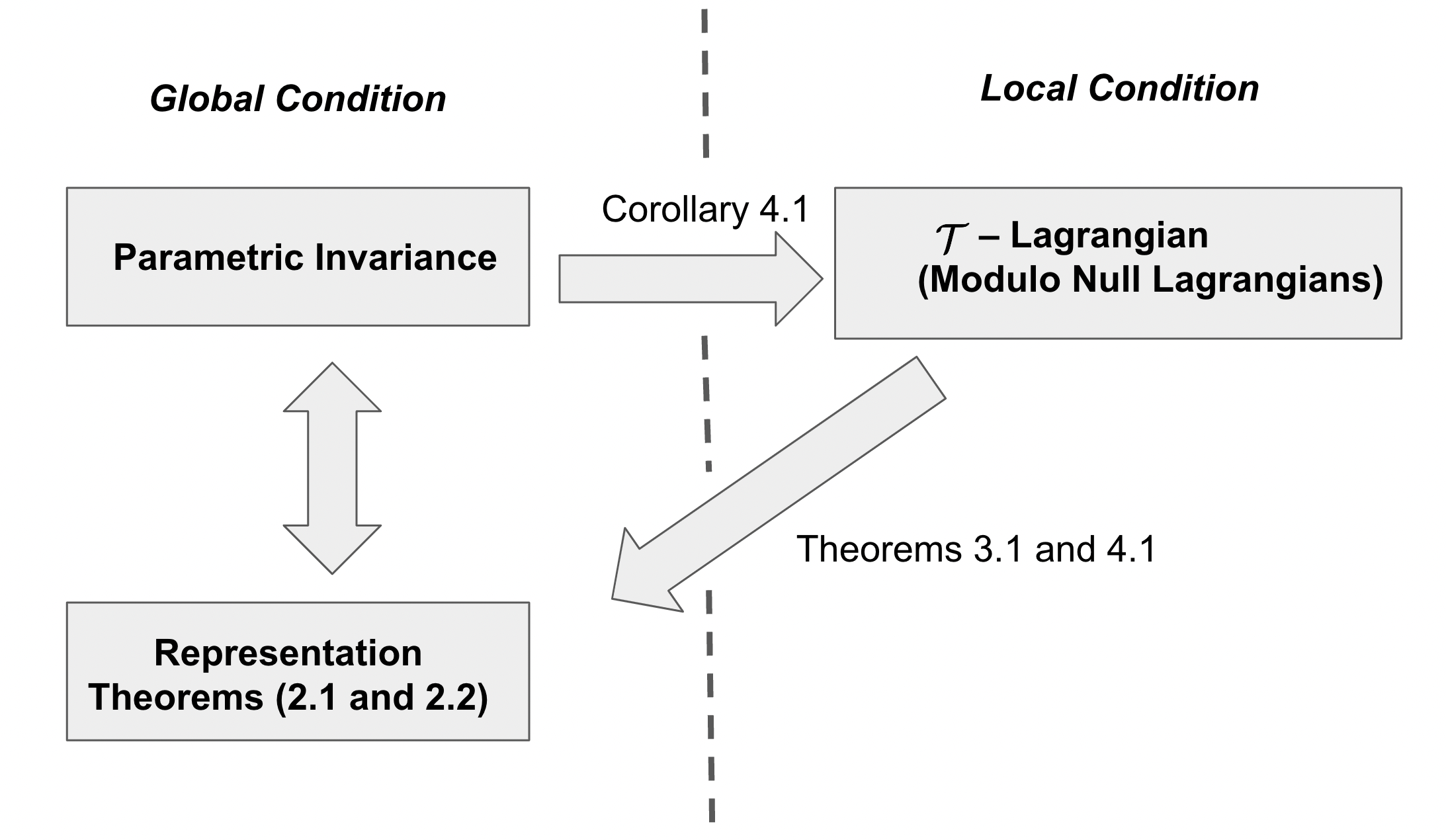
Figure 4: Figure showing the equivalence of parametrization invariance and $\mathcal{T}$-Lagrangian (modulo a null Lagrangian).

We introduce a weakened notion of parametrization invariance that we term as $\mathcal{T}$-Lagrangian. While the representation of functionals that possess parametrization invariance is well known [GH04], and summarized in Theorems 2.1 and 18, we derive the representation results for $\mathcal{T}$-Lagrangian. The significance of the weakened notion is that while parametrization invariance is a global condition on the functional, $\mathcal{T}$-Lagrangian is a local condition that can be enforced at the level of equilibrium equations. We see this in Propositions 21 and 33, where $\mathcal{T}$-Lagrangians are equivalently characterized by vanishing of the tangential component of the Euler-Lagrange equations. Through our results, viz., Theorems 3.1 and 4.1, we see that on one-dimensional domains, for first and second-order, parametrization invariance and $\mathcal{T}$-Lagrangians (modulo Null Lagrangians) are equivalent. This is summarized schematically in Fig. 4. Thus, a global condition on the Lagrangian (i.e., parametrization invariance) can be replaced by a local condition ($\mathcal{T}$-Lagrangian). The complementary concept of $\mathcal{N}$-Lagrangian recovers classical null Lagrangians.

new We emphasize that while the form of the parametrization invariance of the Lagrangian is known in the case $n=2$, our representation theorem 4.1 generalizes this observation for even $\mathcal{T}$-Lagrangians for $n\geq 1$.

In this paper, we utilize the classical framework of the calculus of variations [GFS00]; in other words, we deliberately avoid dwelling on the generalization to weakly differentiable functions and measure-theoretic approach [BCO81, Dac08]. Besides this, except for the use of Poincaré Lemma, we also have avoided the framework of differential geometry and the jet-bundle formalism of variational analysis [Sau89, Gri99, CS05]. These aspects are deemed important in the context of question raised in this paper but are relegated to future investigations.

newFrom certain viewpoint, we have proven that in the one-dimensional setting, our way of weakening the notion of parametrization invariance via $\mathcal{T}$-Lagrangian does not yield any new representations (up to a null Lagrangian). We conjecture that generalizing the results of the paper to higher dimensions as well as higher order Lagrangians ($p>1,\mathcal{L}(\bm{u})=\int_{\Omega}{\mathscr{L}}(\bm{x},\{\nabla^{k}\bm{u}(\bm{x})\}_{k=1}^{p})d{x}$) has non-trivial implications and the links with null Lagrangian are also anticipated [OS88, SB21]. However, the method of the present paper becomes cumbersome in this regard due to the presence of a high number of indices in the expressions as well as the difficulty of integrating some of the partial differential equations.

Appendix A Appendix: Auxiliary Claims

Lemma A.1 .

If ${\mathscr{L}}(s,{\mathbf{u}},{\mathbf{u}}^{\prime},{\mathbf{u}}^{\prime\prime})$ is a $\mathcal{T}$- Lagrangian, then

$$(p_{i}\mathscr{L}_{q_{i}})_{,q_{j}}=0,$$ (65)

$$p_{i}\Big{(}\mathscr{L}_{q_{i}p_{j}}-\mathscr{L}_{p_{i}q_{j}}+2q_{k}\mathscr{L}_{q_{i}q_{j}p_{k}}\Big{)}=0,$$ (66)

for each $j\in\{1,2\}$, where Einstein summation convention is assumed on the repeated indices $i$ and $k$.

Proof Writing (33) explicitly using the Einstein convention, we have

$$p_{i}\Big{(}D_{s}(\mathscr{L}_{q_{i}q_{j}}q_{j}^{\prime}+\mathscr{L}_{q_{i}p_{j}}p_{j}^{\prime}+\mathscr{L}_{q_{i}z_{j}}z_{j}^{\prime}+\mathscr{L}_{q_{i}s}-\mathscr{L}_{p_{i}})+\mathscr{L}_{z_{i}}\Big{)}=0.$$ (67)

Expanding the total derivative, $D_{s}(\cdot)$ and using the notation $z_{k}^{\prime}=p_{k}$, $p_{k}^{\prime}=q_{k}$, we obtain

$$p_{i}\Bigg{(}q_{j}^{\prime\prime}\mathscr{L}_{q_{i}q_{j}}+q_{j}^{\prime}\Big{(}\mathscr{L}_{q_{i}q_{j}q_{k}}q_{k}^{\prime}+\mathscr{L}_{q_{i}q_{j}p_{k}}q_{k}+\mathscr{L}_{q_{i}q_{j}z_{k}}p_{k}+\mathscr{L}_{q_{i}q_{j}s}\Big{)}+\\ \mathscr{L}_{q_{i}p_{j}}q_{j}^{\prime}+q_{j}\Big{(}\mathscr{L}_{q_{i}p_{j}q_{k}}q_{k}^{\prime}+\mathscr{L}_{q_{i}p_{j}p_{k}}q_{k}+\mathscr{L}_{p_{i}p_{j}z_{k}}p_{k}+\mathscr{L}_{q_{i}p_{j}s}\Big{)}+\\ \mathscr{L}_{q_{i}z_{j}}q_{j}+p_{j}\Big{(}\mathscr{L}_{q_{i}z_{j}q_{k}}q_{k}^{\prime}+\mathscr{L}_{q_{i}z_{j}p_{k}}q_{k}+\mathscr{L}_{q_{j}z_{j}z_{k}}p_{k}+\mathscr{L}_{q_{i}z_{j}s}\Big{)}+\\ \Big{(}\mathscr{L}_{q_{i}sq_{k}}q_{k}^{\prime}+\mathscr{L}_{q_{i}sp_{k}}q_{k}+\mathscr{L}_{q_{i}sz_{k}}p_{k}+\mathscr{L}_{q_{i}ss}\Big{)}-\\ \Big{(}\mathscr{L}_{p_{i}q_{k}}q_{k}^{\prime}+\mathscr{L}_{p_{i}p_{k}}q_{k}+\mathscr{L}_{p_{i}z_{k}}p_{k}+\mathscr{L}_{p_{i}s}\Big{)}+\mathscr{L}_{z_{i}}\Bigg{)}=0,$$ (68)

where the first three lines in the previous equation arise from the product rule of the first three terms in brackets of (67), and the next two lines, by applying $D_{s}$ to the last three bracketted terms in (67). Since (68) must hold for all $s$, ${\mathbf{u}}$, $\mathbf{p}$, and $\mathbf{q}$, the coefficient of $q_{j}^{\prime\prime}$ and $q_{j}^{\prime}$ must be zero. Setting the coefficient of $q_{j}^{\prime\prime}$ to zero results in

$$p_{i}\mathscr{L}_{q_{i}q_{j}}=0,$$ (69)

establishing (65). Differentiating the previous equation with respect to $q_{k}$, $z_{k}$, and $s$, respectively, results in the following conditions:

$$p_{i}\mathscr{L}_{q_{i}q_{j}q_{k}}=0,$$ (70)

$$p_{i}\mathscr{L}_{q_{i}q_{j}z_{k}}=0,$$ (71)

$$p_{i}\mathscr{L}_{q_{i}q_{j}s}=0,$$ (72)

where $i,k\in\{1,2\}$. As a consequence of the previous three equations, certain terms in (68) (which appear in terms involving $q_{j}^{\prime}$) vanish. Setting the coefficient of $q_{j}^{\prime}$ to zero, we obtain (66). ∎

Corollary A.1 .

If ${\mathscr{L}}(s,x,y,x^{\prime},y^{\prime})$ is a $\mathcal{T}$-Lagrangian (and therefore has the form (32), where for convenience of notation we write $E_{1}=-E$ and $E_{2}=F$), then the critical points $(x(s),y(s))$ of the (normal-component of the) Euler-Lagrange equation are either constant functions or satisfy

$$E_{,y}(x(s),y(s))+F_{,x}(x(s),y(s))=0.$$ (73)

Proof Recall (32), i.e., according to Theorem 3.1, if ${\mathscr{L}}(s,x,y,x^{\prime},y^{\prime})$ is an $\mathcal{T}$-Lagrangian, then ${\mathscr{L}}$ has the form

$${\mathscr{L}}(s,x,y,x^{\prime},y^{\prime})=\frac{d}{ds}\Psi(s,x(s),y(s))-\big{(}x^{\prime}E(x,y)-y^{\prime}F(x,y)\big{)},$$ (74)

where $\Psi(s,x,y)$, $E(x,y)$, and $F(x,y)$ are arbitrary functions.

Without loss of generality we can ignore the $\Psi$ term as its contribution to the normal component of Euler-Lagrange equation is trivially zero. So, let

$${\mathscr{L}}(s,x,y,x^{\prime},y^{\prime})=x^{\prime}E(x,y)-y^{\prime}F(x,y).$$ (75)

The normal component of this Lagrangian is:

$$\begin{split}&-\big{(}-(E_{,x}x^{\prime}+E_{,y}y^{\prime})+(x^{\prime}E_{,x}-y^{\prime}F_{,x})\big{)}y^{\prime}\\ &+\big{(}(F_{,x}x^{\prime}+F_{,y}y^{\prime})+(x^{\prime}E_{,y}-y^{\prime}F_{,y})\big{)}x^{\prime}=0.\end{split}$$ (76)

Cancelling $E_{,x}$ and $F_{,y}$ terms, we obtain

$$(E_{,y}+F_{,x})(x^{\prime 2}+y^{\prime 2})=0,$$ (77)

i.e.,

$$x^{\prime}=y^{\prime}=0\text{ or }(E_{,y}+F_{,x})(x(s),y(s))=0.$$ (78)

∎

Lemma A.2 .

$\mathbf{p}\cdot f_{,\mathbf{p}}(\mathbf{p})=0$ if and only if $f(\mathbf{p})=g({\bm{\theta}})$, for some function $g$, where ${\bm{\theta}}\in(\mathcal{S}^{1})^{n-1}$.

Proof

Let us first recall that every vector $\hat{\mathbf{p}}\in\mathcal{S}^{n-1}$ can be associated with a ${\bm{\theta}}\in{(\mathcal{S}^{1})^{n-1}}$, where ${\bm{\theta}}=(\theta_{1},\theta_{2},\dotsc,\theta_{n-1})$ in (23c) (schematically shown in Fig. 3).

Also note that by Euler’s theorem for homogeneous functions, a function $f(\mathbf{p})$ satisfies the partial differential equation

$$\mathbf{p}\cdot f_{,\mathbf{p}}=0,$$ (79)

iff $f(\mathbf{p})$ is homogeneous in $\mathbf{p}$ of degree $0$. Consider the change of variables:

$$\mathbf{p}(r,{\bm{\theta}})=r{\hat{\mathbf{p}}}({\bm{\theta}}),\quad{\hat{\mathbf{p}}}({\bm{\theta}})\cdot{\hat{\mathbf{p}}}({\bm{\theta}})=1.$$ (80)

where, ${\hat{\mathbf{p}}}({\bm{\theta}})$ is locally described in terms of $n-1$ coordinates $\theta_{i}\in\mathcal{S}^{1}$, $i=1,\dotsc,n-1$ noted above. It follows that

$$f_{,r}={\mathbf{p}}_{,r}[f_{,\mathbf{p}}]={\mathbf{p}}_{,r}\cdot f_{,\mathbf{p}},\;f_{,{\bm{\theta}}}=({\mathbf{p}}_{,{\bm{\theta}}})^{T}[f_{,\mathbf{p}}].$$ (81)

The second equation, in components, is $f_{,\theta_{i}}=f_{,p_{j}}p_{j,\theta_{i}}.$ Since $\mathbf{p}_{,r}={\hat{\mathbf{p}}}({\bm{\theta}})$, $({\mathbf{p}}_{,{\bm{\theta}}})^{T}[{\hat{\mathbf{p}}}({\bm{\theta}})]=\mathbf{0}$ (second equation, in components, holds as $p_{k}p_{k}=r^{2}$ so that $p_{k,\theta_{i}}p_{k}=0$), we have

$$rf_{,r}=f_{,\mathbf{p}}\cdot\mathbf{p},\;f_{,{\bm{\theta}}}=({\mathbf{p}}_{,{\bm{\theta}}})^{T}[f_{,\mathbf{p}}].$$

Due to (79), we have

$$rf_{,r}=0\implies f=g_{1}({\bm{\theta}}),\;\text{ for some function }g_{1}\text{ of }{\bm{\theta}}.$$

∎

Lemma A.3 .

$\hat{\mathbf{p}}_{,\theta_{i}}({\bm{\theta}})\cdot f_{,\mathbf{p}}=0$ for $i=1,\dotsc,n-1$ if and only if $f=g(\sqrt{\mathbf{p}\cdot\mathbf{p}})$, for some function $g$.

Proof Consider the change of variables:

$$\mathbf{p}(r,{\bm{\theta}})=r{\hat{\mathbf{p}}}({\bm{\theta}}),\quad{\hat{\mathbf{p}}}({\bm{\theta}})\cdot{\hat{\mathbf{p}}}({\bm{\theta}})=1.$$ (82)

It follows by differentiating $f$ that

$$f_{,{\bm{\theta}}}=(\mathbf{p}_{,{\bm{\theta}}})^{T}[f_{,\mathbf{p}}].$$ (83)

That is, for each $i=1,\dotsc n-1$, we have

$$f_{,\theta_{i}}=r\hat{\mathbf{p}}_{,\theta_{i}}\cdot f_{,\mathbf{p}}=0,$$ (84)

where the last equality follows from the hypothesis. Thus, $f$ is independent of ${\bm{\theta}}$ and must only depend on $r=\sqrt{\mathbf{p}\cdot\mathbf{p}}$. ∎

Appendix B Claims from Second Order Theory

Recall the change of variables given by (39d) and their inverse (40b). Taking the derivatives of $\mathbf{p}$ and $\mathbf{q}$ (as given by the inverse maps (40b)) with respect to $r$, $\bm{\theta}$, $\xi$, and $\bm{\eta}$, we obtain:

$$\mathbf{p}_{,r} = \hat{\mathbf{p}}(\bm{\theta}),$$ (85a)

$$\mathbf{q}_{,r} = \xi\hat{\mathbf{p}}+\hat{\mathbf{p}}_{,\bm{\theta}}\bm{\eta},$$ (85b)

$$\mathbf{p}_{,\bm{\theta}} = r\hat{\mathbf{p}}_{,\bm{\theta}},$$ (85c)

$$\mathbf{p}_{,\xi} = \mathbf{0},$$ (85d)

$$\mathbf{q}_{,\xi} = r\hat{\mathbf{p}}\quad(=\mathbf{p}),$$ (85e)

$$\mathbf{p}_{,\bm{\eta}} = \mathbf{O},$$ (85f)

$$\mathbf{q}_{,\bm{\eta}} = r\hat{\mathbf{p}}_{,\bm{\theta}},$$ (85g)

where $\mathbf{O}$ is a zero matrix (of appropriate dimension)

Lemma B.1 .

If $\mathscr{L}(s,{\mathbf{u}},\mathbf{p},\mathbf{q})$ is a function of the indicated variables, then, in terms of the new variables defined by (39d), we have the following identity:

$$\mathbf{p}\cdot\mathscr{L}_{\mathbf{p}}+2\mathbf{q}\cdot\mathscr{L}_{\mathbf{q}}=r\mathscr{L}_{,r}+\xi\mathscr{L}_{,\xi}+\bm{\eta}\cdot\mathscr{L}_{,\bm{\eta}}$$ (86)

Proof By inspection of (85a)–(85g), let us first note that $\mathbf{p}$ and $\mathbf{q}$ (recall (39d) and (40b)) both depend on $r$ and $\bm{\theta}$, while only $\mathbf{q}$ depends on $\xi$ and $\bm{\eta}$.

By the chain rule, it follows that,

$$\mathscr{L}_{,r}=\mathbf{p}_{,r}\cdot\mathscr{L}_{,\mathbf{p}}+\mathbf{q}_{,r}\cdot\mathscr{L}_{,\mathbf{q}}=\hat{\mathbf{p}}\cdot\mathscr{L}_{,\mathbf{p}}+\xi\hat{\mathbf{p}}\cdot\mathscr{L}_{,\mathbf{q}}+(\hat{\mathbf{p}}_{,\bm{\theta}}\bm{\eta})\cdot\mathscr{L}_{,\mathbf{q}},$$

where the second equality follows from (85a) and (85b). Multiplying both sides by $r$ and using $\mathbf{p}=r\hat{\mathbf{p}}$ and (40b) in the last term, we obtain

$$r\mathscr{L}_{,r}=\mathbf{p}\cdot\mathscr{L}_{,\mathbf{p}}+r\xi\hat{\mathbf{p}}\cdot\mathscr{L}_{,\mathbf{q}}+(\mathbf{q}-r\xi\hat{\mathbf{p}})\cdot\mathscr{L}_{,\mathbf{q}}.$$ (87)

Similarly, using (85d) and (85e), we obtain

$$\xi\mathscr{L}_{,\xi}=\xi\mathbf{p}\cdot\mathscr{L}_{,\mathbf{q}}.$$ (88)

Finally, differentiating $\mathscr{L}$ with respect to $\bm{\eta}$ and using (85f) and (85g), we obtain:

$$\mathscr{L}_{,\bm{\eta}}=\mathbf{p}_{,\bm{\eta}}^{T}[\mathscr{L}_{,\mathbf{p}}]+\mathbf{q}_{,\bm{\eta}}^{T}[\mathscr{L}_{,\mathbf{q}}]=r\hat{\mathbf{p}}^{T}_{,\bm{\theta}}[\mathscr{L}_{,\mathbf{q}}]$$

Dotting both sides with $\bm{\eta}$, we obtain

$$\bm{\eta}\cdot\mathscr{L}_{,\bm{\eta}}=\bm{\eta}\cdot r\hat{\mathbf{p}}^{T}_{,\bm{\theta}}[\mathscr{L}_{,\mathbf{q}}]=(r\hat{\mathbf{p}}_{,\bm{\theta}}\bm{\eta})\cdot\mathscr{L}_{,\mathbf{q}}=(\mathbf{q}-r\xi\hat{\mathbf{p}})\cdot\mathscr{L}_{,\mathbf{q}},$$ (89)

where the second equality follows from the definition of the transpose of matrix and the last equality from (40b). Combining (87), (88), and (89), we obtain:

$$r\mathscr{L}_{,r}+\xi\mathscr{L}_{,\xi}+\bm{\eta}\cdot\mathscr{L}_{,\bm{\eta}}=\mathbf{p}\cdot\mathscr{L}_{,\mathbf{p}}+2\mathbf{q}\cdot\mathscr{L}_{,\mathbf{q}}.$$

∎

The following proposition is a consequence of the previous lemma.

Proposition B.1 .

In terms of the new variables defined by (39d), the Lagrangian must satisfy the condition,

$$r\mathscr{L}_{,r}+\bm{\eta}\cdot\mathscr{L}_{,\bm{\eta}}-\mathscr{L}=\xi(r\hat{A}_{,r}-\hat{A})+\bm{\eta}\cdot\hat{A}_{,\bm{\theta}}+\hat{B},$$ (90)

where $\hat{A}$ and $\hat{B}$ are defined in (41) and (42), respectively.

Proof Note that $A$ and $B$ on the right side of (37) are independent of $\mathbf{q}$. That is, their polar forms are independent of $\xi$ and $\bm{\eta}$, c.f., (41), (42). It follows by chain rule that,

$$r\hat{A}_{,r}=\mathbf{p}\cdot A_{,\mathbf{p}}$$

$$\hat{A}_{,\bm{\theta}}=r(\hat{\mathbf{p}}^{T}_{,\bm{\theta}})A_{,\mathbf{p}}$$

Combining the previous two equations as follows, we obtain

$$\xi rA_{,r}+\bm{\eta}\cdot A_{,\bm{\theta}}=\xi\mathbf{p}\cdot A_{,\mathbf{p}}+(\mathbf{q}-\xi\mathbf{p})\cdot\mathbf{A}_{,\mathbf{p}}=\mathbf{q}\cdot\mathbf{A}_{,\mathbf{p}},$$ (91)

where we have used (40b) to replace $\bm{\eta}$ in terms of $\mathbf{q}$.

Using the Lemma 86, the left hand (37) of Lemma 37 can be written as $r\mathscr{L}_{,r}+\xi\mathscr{L}_{,\xi}+\bm{\eta}\cdot\mathscr{L}_{,\bm{\eta}}-\mathscr{L}$. Using (91) in the right side of (37) along with (45), i.e., $\mathscr{L}_{,\xi}=\hat{A}$, we deduce the require result. ∎

The following proposition is used in Theorem 4.1.

Proposition B.2 .

If the Lagrangian has the form (52), that is,

$$\mathscr{L}=D_{s}\mathcal{A}+Q(s,\mathbf{u},r,\bm{\theta})+rE(s,\mathbf{u},\bm{\theta},\frac{\bm{\eta}}{r}),$$

then if $\mathscr{L}$ satisfies the $\mathcal{T}$-Lagrangian condition (33), then $Q$ and $E$ must satisfy the condition:

$$\bm{\eta}\cdot Q_{,\bm{\theta}}-r\Big{(}\bm{\eta}\cdot Q_{,r\bm{\theta}}+r\xi Q_{,rr}-\hat{\mathbf{p}}(\bm{\theta})\cdot Q_{,{\mathbf{u}}}+\mathbf{p}Q_{,r{\mathbf{u}}}+Q_{,sr}\Big{)}-rE_{,s}=0.$$ (92)

Proof By repeated application of product rule for derivatives and using $\mathbf{q}=\mathbf{p}^{\prime}$, the three terms in (33) can be individually simplified as follows:

$$\mathbf{p}\cdot D_{ss}\mathscr{L}_{\mathbf{q}}=D_{s}(\mathbf{p}\cdot D_{s}\mathscr{L}_{\mathbf{q}})-\mathbf{q}\cdot D_{s}\mathscr{L}_{\mathbf{q}}=D_{s}(\mathbf{p}\cdot D_{s}\mathscr{L}_{\mathbf{q}})-D_{s}(\mathbf{q}\cdot\mathscr{L}_{\mathbf{q}})+\mathbf{q}^{\prime}\cdot\mathscr{L}_{\mathbf{q}}$$

$$-\mathbf{p}\cdot D_{s}\mathscr{L}_{\mathbf{p}}=-D_{s}(\mathbf{p}\cdot\mathscr{L}_{\mathbf{p}})+\mathbf{q}\cdot\mathscr{L}_{\mathbf{p}}$$

$$\mathbf{p}\cdot\mathscr{L}_{\mathbf{u}}=D_{s}\mathscr{L}-\mathscr{L}_{s}-\mathbf{q}\cdot\mathscr{L}_{\mathbf{p}}-\mathbf{q}^{\prime}\cdot\mathscr{L}_{\mathbf{q}},$$

where the last equation follows from chain rule. Adding the previous three equations, we see that the $\mathcal{T}$–Lagrangian condition (33) can be written as

$$D_{s}\Big{(}\mathbf{p}\cdot D_{s}\mathscr{L}_{\mathbf{q}}-\mathbf{q}\cdot\mathscr{L}_{\mathbf{q}}-\mathbf{p}\cdot\mathscr{L}_{\mathbf{p}}+\mathscr{L}\Big{)}-\mathscr{L}_{s}\equiv 0.$$

Using $\mathbf{p}\cdot D_{s}\mathscr{L}_{\mathbf{q}}=D_{s}(\mathbf{p}\cdot\mathscr{L}_{\mathbf{q}})-\mathbf{q}\cdot\mathscr{L}_{\mathbf{q}}$, we obtain

$$D_{s}\Big{(}D_{s}(\mathbf{p}\cdot\mathscr{L}_{\mathbf{q}})-2\mathbf{q}\cdot\mathscr{L}_{\mathbf{q}}-\mathbf{p}\cdot\mathscr{L}_{\mathbf{p}}+\mathscr{L}\Big{)}-\mathscr{L}_{s}\equiv 0.$$ (93)

Since the first term in (52) is a null Lagrangian, we can neglect it when we plug in the Lagrangian into (93).

Note that, neglecting the null Lagrangian term, $\mathscr{L}$ is independent of $\xi$ (c.f., (52)), i.e., $\mathscr{L}_{,\xi}=0$. Thus, it follows from Lemma 86 that

$$\mathbf{p}\cdot\mathscr{L}_{\mathbf{p}}+2\mathbf{q}\cdot\mathscr{L}_{\mathbf{q}}-\mathscr{L}=r\mathscr{L}_{,r}+\bm{\eta}\cdot\mathscr{L}_{\bm{\eta}}-\mathscr{L}.$$ (94)

Curiously, if $\mathscr{L}=Q+rE$, then,

$$\mathbf{p}\cdot\mathscr{L}_{\mathbf{q}}\equiv 0.$$ (95)

To see this first note that

$$r\hat{\mathbf{p}}(\bm{\theta})\bm{\eta}_{,\mathbf{q}}=\mathbf{I}-\hat{\mathbf{p}}\otimes\hat{\mathbf{p}},$$

which follows from differentiating (39d) with respect to $\mathbf{q}$. Thus, $\bm{\eta}_{,\mathbf{q}}[\mathbf{p}]=\mathbf{0}$. Since $Q$ is independent of $\mathbf{q}$, $\mathscr{L}_{\mathbf{q}}=\bm{\eta}_{\mathbf{q}}^{T}[E_{,\bm{\eta}}]$. Thus,

$$\mathbf{p}\cdot\mathscr{L}_{\mathbf{q}}=\mathbf{p}\cdot\bm{\eta}_{,\mathbf{q}}^{T}E_{,\bm{\eta}}=\bm{\eta}_{,\mathbf{q}}[\mathbf{p}]\cdot E_{,\bm{\eta}}=0.$$

Returning to (93) along with (94), we can simplify the former equation to

$$D_{s}\Big{(}-r\mathscr{L}_{,r}-\mathbf{\eta}\cdot\mathbf{\mathscr{L}}_{,\mathbf{\eta}}+\mathscr{L}\Big{)}-\mathscr{L}_{s}\equiv 0.$$

Plugging in $\mathscr{L}=Q+rE$ in the the previous equation established the required result (92). ∎

References

[Eul44]Leonhard Euler
“Methodus inveniendi lineas curvas maximi minimive proprietate gaudentes sive solutio problematis isoperimetrici latissimo sensu accepti”
chapter Additamentum 1. eulerarchive.org E065, 1744
[Lov27]Augustus Edward Hough Love
“A treatise on the mathematical theory of elasticity”
University press, 1927
[CH58]John W Cahn and John E Hilliard
“Free energy of a nonuniform system. I. Interfacial free energy”
In The Journal of chemical physics28.2American Institute of Physics, 1958, pp. 258–267
[Ede62]Dominic GB Edelen
“The null set of the Euler-Lagrange operator”
In Archive for Rational Mechanics and Analysis11.1Springer, 1962, pp. 117–121
[Eri62]JL Ericksen
“Nilpotent energies in liquid crystal theory”
In Archive for Rational Mechanics and Analysis10.1Springer, 1962, pp. 189–196
[Run66]Hanno Rund
“The Hamilton-Jacobi theory in the calculus of variations: its role in mathematics and physics”
Krieger Publishing Company, 1966
[Can70]Peter B Canham
“The minimum energy of bending as a possible explanation of the biconcave shape of the human red blood cell”
In Journal of theoretical biology26.1Elsevier, 1970, pp. 61–81
[Hel73]Wolfgang Helfrich
“Elastic properties of lipid bilayers: theory and possible experiments”
In Zeitschrift für Naturforschung C28.11-12Verlag der Zeitschrift für Naturforschung, 1973, pp. 693–703
[Nag73]Paul Mansour Naghdi
“The theory of shells and plates”
In Linear theories of elasticity and thermoelasticitySpringer, 1973, pp. 425–640
[She75]Ping Sheng
“Introduction to the elastic continuum theory of liquid crystals”
In Introduction to Liquid CrystalsSpringer, 1975, pp. 103–127
[AT76]Frederick J Almgren and Jean E Taylor
“The geometry of soap films and soap bubbles”
In Scientific American235.1JSTOR, 1976, pp. 82–93
[BCO81]John M Ball, JC Currie and Peter J Olver
“Null Lagrangians, weak continuity, and variational problems of arbitrary order”
In Journal of Functional Analysis41.2Elsevier, 1981, pp. 135–174
[Gur82]Morton E Gurtin
“An introduction to continuum mechanics”
Academic press, 1982
[HS86]Gary T Horowitz and Andrew Strominger
“Origin of gauge invariance in string theory”
In Physical review letters57.5APS, 1986, pp. 519
[Olv86]Peter J Olver
“Noether’s theorems and systems of Cauchy–Kovalevskaya type”
In Nonlinear Systems of Partial Differential Equations in Applied Mathematics23Am. Math. Soc., 1986, pp. 81–104
[BDM87]SA Brazovskii, IE Dzyaloshinskii and AR Muratov
“Theory of weak crystallization”
In Sov. Phys. JETP66.3, 1987, pp. 625
[OS88]Peter J Olver and J Sivaloganathan
“The structure of null Larangians”
In Nonlinearity1.2IOP Publishing, 1988, pp. 389
[Sau89]David J Saunders
“The geometry of jet bundles”
Cambridge University Press, 1989
[Nor93]John D Norton
“General covariance and the foundations of general relativity: eight decades of dispute”
In Reports on progress in physics56.7IOP Publishing, 1993, pp. 791
[FGT99]Geza Fulop, Dmitri Maximovitch Gitman and IV Tyutin
“Reparametrization invariance as gauge symmetry”
In International journal of theoretical physics38.7Springer, 1999, pp. 1941–1968
[Gri99]Dan Radu Grigore
“Variationally trivial Larangians and locally variational differential equations of arbitrary order”
In Differential Geometry and its Applications10.1Elsevier, 1999, pp. 79–105
[GFS00]IM Gelfand, SV Fomin and RA Silverman
“Calculus of variations (Unabridged repr. ed.)”
Dover Publications, Mineola, New York, 2000
[TMW00]Kip S Thorne, Charles W Misner and John Archibald Wheeler
“Gravitation”
Freeman, 2000
[CG02]Riccardo Capovilla and Jemal Guven
“Stresses in lipid membranes”
In Journal of Physics A: Mathematical and General35.30IOP Publishing, 2002, pp. 6233
[Ste+03]David Steigmann et al.
“On the variational theory of cell-membrane equilibria”
In Interfaces and Free Boundaries5.4, 2003, pp. 357–366
[GH04]Mariano Giaquinta and Stefan Hildebrandt
“The First Variation”
In Calculus of Variations ISpringer, 2004, pp. 3–86
[NPW04]David Nelson, Tsvi Piran and Steven Weinberg
“Statistical mechanics of membranes and surfaces”
World Scientific, 2004
[CS05]Michael Crampin and DJ Saunders
“On null Larangians”
In Differential Geometry and its Applications22.2Elsevier, 2005, pp. 131–146
[Dac08]B Dacorogna
“Direct methods in the calculus of variations Second edition”
In Applied Mathematical Sciences78.2Springer ScienceMedia, 2008
[Des09]Markus Deserno
“Mesoscopic Membrane Physics: Concepts, Simulations, and Selected Applications”
In Macromolecular Rapid Communications30.9-10, 2009, pp. 752–771
[CM11]Tobias H Colding and William P Minicozzi
“A course in minimal surfaces”
American Mathematical Soc., 2011
[HM11]Peter E Hydon and Elizabeth L Mansfield
“Extensions of Noether’s second theorem: from continuous to discrete systems”
In Proceedings of the Royal Society A: Mathematical, Physical and Engineering Sciences467.2135The Royal Society Publishing, 2011, pp. 3206–3221
[KS12]Ernst Kuwert and Reiner Schätzle
“The Willmore functional”
In Topics in modern regularity theorySpringer, 2012, pp. 1–115
[BCS16]Larry Bates, Robin Chhabra and Jedrzej Sniatycki
“Elastica as a dynamical system”
In Journal of Geometry and Physics110Elsevier, 2016, pp. 348–381
[Dha+16]Sanjay Dharmavaram et al.
“Landau theory and the emergence of chirality in viral capsids”
In Europhysics Letters116.2IOP Publishing, 2016, pp. 26002
[Nes+18]Michael Nestler, Ingo Nitschke, Simon Praetorius and Axel Voigt
“Orientational order on surfaces: The coupling of topology, geometry, and dynamics”
In Journal of Nonlinear Science28Springer, 2018, pp. 147–191
[NRV20]Ingo Nitschke, Sebastian Reuther and Axel Voigt
“Liquid crystals on deformable surfaces”
In Proceedings of the Royal Society A476.2241The Royal Society Publishing, 2020, pp. 20200313
[BW21]Juan Pablo Borthagaray and Shawn W Walker
“The Q-tensor model with uniaxial constraint”
In Handbook of Numerical Analysis22Elsevier, 2021, pp. 313–382
[GM21]Vesselin G Gueorguiev and Andre Maeder
“Reparametrization Invariance and Some of the Key Properties of Physical Systems”
In Symmetry13.3Multidisciplinary Digital Publishing Institute, 2021, pp. 522
[SB21]Basant Lal Sharma and Nirupam Basak
“Null lagrangians in Cosserat elasticity”
In Journal of Elasticity143Springer, 2021, pp. 337–358