Reinforcement Learning With Reward Machines in Stochastic Games

Abstract

We investigate multi-agent reinforcement learning for stochastic games with complex tasks, where the reward functions are non-Markovian. We utilize reward machines to incorporate high-level knowledge of complex tasks. We develop an algorithm called Q-learning with reward machines for stochastic games (QRM-SG), to learn the best-response strategy at Nash equilibrium for each agent. In QRM-SG, we define the Q-function at a Nash equilibrium in augmented state space. The augmented state space integrates the state of the stochastic game and the state of reward machines. Each agent learns the Q-functions of all agents in the system. We prove that Q-functions learned in QRM-SG converge to the Q-functions at a Nash equilibrium if the stage game at each time step during learning has a global optimum point or a saddle point, and the agents update Q-functions based on the best-response strategy at this point. We use the Lemke-Howson method to derive the best-response strategy given current Q-functions. The three case studies show that QRM-SG can learn the best-response strategies effectively. QRM-SG learns the best-response strategies after around 7500 episodes in Case Study I, 1000 episodes in Case Study II, and 1500 episodes in Case Study III, while baseline methods such as Nash Q-learning and MADDPG fail to converge to the Nash equilibrium in all three case studies.

1 Introduction

In games, multiple agents interact with each other and the behavior of each agent can affect the performance of other agents. Multi-agent reinforcement learning (MARL) [1] is a framework for multiple agents to optimize their strategies by repeatedly interacting with the environment. The interactions between agents in MARL problems can be modeled as a stochastic game (SG), where Nash equilibrium can be a solution concept. In a Nash equilibrium, agents have best-response strategies considering other agents’ actions.

In many complex games, the reward functions are non-Markovian (i.e., the reward of each agent can depend on the history of events). One way of encoding a non-Markovian reward function is by using a type of Mealy machine named reward machines [2]. In this paper, we focus on stochastic games where each agent intends to complete a complex task which can be represented by a reward machine capturing the temporal structure of the reward function.

We introduce a variant of the PAC-MAN game as a motivational example, where two agents try to capture each other, and the task completion is defined based on complex conditions, as illustrated in Figure 1. Two agents and evolve in a grid-world by taking synchronous steps towards adjacent cells. We also introduce two power bases and at fixed locations. We track whether the two agents encounter logical propositions such as , , and or not to evaluate the lower-level dynamics and specify the high-level reward. For instance, the proposition is true when agent is at power base . Similarly, the proposition is true when agents and meet on the same cell. In the simplest variant of the game, the goal of each agent is to first reach its own power base and then capture the other agent. Each agent obtains a reward of 1 when its task is completed. Whenever agent arrives at its power base , agent becomes more powerful than agent . However, if agent then arrives at its power base , agent becomes the more powerful agent. The more powerful agent is capable to capture the other agent.

We address the challenge of learning complex tasks in two-agent general-sum stochastic games with non-Markovian reward functions. We develop an algorithm called Q-learning with reward machines for stochastic games (QRM-SG), where we use reward machines to specify the tasks and expose the structure of reward functions. The proposed approach defines the Q-function at a Nash equilibrium in augmented state space to adapt Q-learning to the setting of stochastic games when the tasks are specified by reward machines. The augmented state space integrates the state of the stochastic game and the state of reward machines. During learning, we formulate a stage game at each time step based on the current Q-functions in augmented state space and use the Lemke-Howson method [3] to derive a Nash equilibrium. Q-functions in augmented state space are then updated according to the Nash equilibrium. QRM-SG enables the learning of the best-response strategy at a Nash equilibrium for each agent. Q-functions learned in QRM-SG converge to the Q-functions at a Nash equilibrium if the stage game at each time step during learning has a global optimum point or a saddle point, and the agents update Q-functions based on the best-response strategy at this point. We test QRM-SG in three case studies and compare QRM-SG with common baselines such as Nash Q learning [4], Nash Q-learning in augmented state space, multi-agent deep deterministic policy gradient (MADDPG) [5], and MADDPG in augmented state space. The results show that QRM-SG learns the best-response strategies at a Nash equilibrium effectively.

(a) Map of the environment. Agents and can move synchronously to an adjacent cell (or stay put) at each step. Locations and are called power bases.

(b) Reward machine for agent with sparse reward (zero when not specified on a transition). We suppose that , and cannot all be true at the same time, making this reward machine deterministic. $\top$ represents tautology.

Figure 1: The simplest variant of the PAC-MAN game is a symmetric zero-sum game where two agents try to capture each other. The agent that visited its own power base the most recently can capture the other agent. The low-level stochastic game plays out in a grid world (1(a)) and the high-level reward is captured by (1(b)).

2 Related Work

Multi-agent reinforcement learning with stochastic games: Our work is closely related to multi-agent reinforcement learning in stochastic games. Many recent works of multi-agent reinforcement learning (MARL) focus on a cooperative setting  [6, 7, 8, 9, 10, 11, 12, 13], where all the agents share a common reward function. [8] addresses the nonstationarity issue introduced by independent Q-learning in multi-agent reinforcement learning by using the importance sampling technique since the multiple agents usually learn concurrently. With the multi-agent actor-critic method as a backbone, [11] proposes counterfactual multi-agent (COMA) policy gradients that use a centralized critic to estimate the Q-function and decentralized actors to optimize the agents’ policies. Similar to both of these approaches that describe the multi-agent task in the stochastic game, but we tackle a non-cooperative multi-agent reinforcement learning problem in a stochastic game compared to  [14, 15, 16, 17]. As opposed to [14, 15], which extends inverse reinforcement learning (IRL) to the non-cooperative stochastic game to let the agent learn the reward function from the observation of other agent/expert’s behavior, we assume the reward function is given to all agents that participate in the stochastic game. However, our work shares the same objective as the works mentioned above, as each agent learns a policy at a Nash equilibrium in the stochastic game. Furthermore, the existing works rely on the Markovian property of the reward function. The definition of the stochastic game in this paper differs from the aforementioned works as we specify the reward function as non-Markovian, which is more applicable to many real-world applications.

Reinforcement learning with formal methods: This paper is also closely related to the work of using the formal methods in reinforcement learning (RL) with a non-Markovian reward function for single agent  [18, 19, 20, 21, 22, 23, 24, 25, 26], and multi-agent [27, 28]. In the single-agent RL, [18] proposes DeepSynth which is a new algorithm that synthesizes deterministic finite automation to infer the unknown non-Markovian rewards of achieving a sequence of high-level objectives. However, DeepSynth is based on the general Markov decision process, which makes it incapable of solving MARL problems that are modeled as a stochastic game. In a similar case for multi-agent reinforcement learning, [27] tackles the MARL problem in a stochastic game with non-Markovian reward expressed in temporal logic. [28] incorporate the non-Markovian reward to MARL in an unknown environment, with the complex task specification also described in temporal logic. In this work, the reward function for all the agents in a stochastic game is encoded by the reward machine, which provides an automata-based representation that enables an agent to decompose an RL problem into structured subproblems that can be efficiently learned via off-policy learning[2].

3 Preliminaries

In this section, we introduce the necessary background on stochastic games, reward machines, and how to connect stochastic games and reward machines.

3.1 Stochastic Games

Definition 1.

A two-player general-sum stochastic game (SG) is a tuple $\mathcal{G}=(S,s_{I},A_{\mathfrak{e}},A_{\mathfrak{a}},p,R_{\mathfrak{e}},R_{\mathfrak{a}},\gamma)$, where $S$ is the finite state space (consisting of states $s=[s_{\mathfrak{e}};s_{\mathfrak{a}}]$, $s_{\mathfrak{e}}$ and $s_{\mathfrak{a}}$ are the substates of the ego agent and the adversarial agent, respectively), $s_{I}\in S$ is the initial state, $A_{\mathfrak{e}}$ and $A_{\mathfrak{a}}$ are the finite set of actions for the ego agent and the adversarial agent, respectively, and $p\colon S\times A_{\mathfrak{e}}\times A_{\mathfrak{a}}\times S\rightarrow[0,1]$ is the probabilistic transition function. Reward functions $R_{\mathfrak{e}}:(S\times A_{\mathfrak{e}}\times A_{\mathfrak{a}})^{+}\times S\rightarrow\mathbb{R}$ and $R_{\mathfrak{a}}:(S\times A_{\mathfrak{e}}\times A_{\mathfrak{a}})^{+}\times S\rightarrow\mathbb{R}$ specify the non-Markovian rewards to the ego and adversarial agents, respectively. $\gamma\in(0,1]$ is the discount factor.

We use the subscripts $\mathfrak{e}$ and $\mathfrak{a}$ to represent the ego agent and the adversarial agent, respectively. Our definition of the SG differs from the “usual” definition used in reinforcement learning (e.g., [29]) in that the reward functions $R_{\mathfrak{e}}$ and $R_{\mathfrak{a}}$ are defined over the whole history (i.e., the rewards are non-Markovian). A trajectory is a sequence of states and actions $s_{0}a_{\mathfrak{e},0}a_{\mathfrak{a},0}s_{1}\ldots s_{k}a_{\mathfrak{e},k}a_{\mathfrak{a},k}s_{k+1}$, with $s_{0}=s_{I}$. Its corresponding reward sequence for agent $\mathfrak{i}$ ($\mathfrak{i}\in\{\mathfrak{e},\mathfrak{a}\}$) is $r_{\mathfrak{i},1}\ldots r_{\mathfrak{i},k}$, where $r_{\mathfrak{i},t}=R_{\mathfrak{i}}(s_{0}a_{\mathfrak{e},0}a_{\mathfrak{a},0}\ldots s_{t}a_{\mathfrak{e},t}a_{\mathfrak{a},t}s_{t+1})$, for each $t\leq k$. For both the ego agent and the adversarial agent, they observe the same trajectory $s_{0}a_{\mathfrak{e},0}a_{\mathfrak{a},0}\ldots s_{k}a_{\mathfrak{e},k}a_{\mathfrak{a},k}s_{k+1}$. The ego agent achieves a discounted cumulative reward $\sum_{t=0}^{k}\gamma^{t}r_{\mathfrak{e},t}$ for the trajectory $s_{0}a_{\mathfrak{e},0}a_{\mathfrak{a},0}\ldots s_{k}a_{\mathfrak{e},k}a_{\mathfrak{a},k}s_{k+1}$. Similarly, the adversarial agent achieves a discounted cumulative reward $\sum_{t=0}^{k}\gamma^{t}r_{\mathfrak{a},t}$ for the trajectory $s_{0}a_{\mathfrak{e},0}a_{\mathfrak{a},0}\ldots s_{k}a_{\mathfrak{e},k}a_{\mathfrak{a},k}s_{k+1}$.

In an SG, we consider each agent to be equipped with a Markovian strategy $\pi_{\mathfrak{i}}:S\times A_{\mathfrak{i}}\rightarrow[0,1],\mathfrak{i}\in\{\mathfrak{e},\mathfrak{a}\}$, mapping the state to the probability of selecting each possible action. The objective of the ego agent and the adversarial agent is to maximize the expected discounted cumulative reward $\tilde{v}_{\mathfrak{e}}$ and $\tilde{v}_{\mathfrak{a}}$, respectively.

$$\tilde{v}_{\mathfrak{i}}(s,\pi_{\mathfrak{e}},\pi_{\mathfrak{a}})=\sum_{t=0}^{\infty}\gamma^{t}\mathbb{E}(r_{\mathfrak{i},t}|\pi_{\mathfrak{e}},\pi_{\mathfrak{a}},s_{0}=s)$$ (1)

As a solution concept of an SG, a Nash equilibrium [30] is a collection of strategies for each of the agents such that each agent cannot improve its own reward by changing its own strategy, or we say that, each agent’s strategy is a best-response to the other agents’ strategies.

Definition 2.

For an SG $\mathcal{G}=(S,s_{I},A_{\mathfrak{e}},A_{\mathfrak{a}},R_{\mathfrak{e}},R_{\mathfrak{a}},p,\gamma)$, the strategies of the ego agent and the adversarial agent $\pi^{\ast}_{\mathfrak{e}}$ and $\pi^{\ast}_{\mathfrak{a}}$ are at a Nash equilibrium of the SG if

$$\begin{split}\tilde{v}_{\mathfrak{e}}(s,\pi^{\ast}_{\mathfrak{e}},\pi^{\ast}_{\mathfrak{a}})&\geq\tilde{v}_{\mathfrak{e}}(s,\pi_{\mathfrak{e}},\pi^{\ast}_{\mathfrak{a}})\\ \tilde{v}_{\mathfrak{a}}(s,\pi^{\ast}_{\mathfrak{e}},\pi^{\ast}_{\mathfrak{a}})&\geq\tilde{v}_{\mathfrak{a}}(s,\pi^{\ast}_{\mathfrak{e}},\pi_{\mathfrak{a}})\end{split}$$

hold for any $\pi_{\mathfrak{e}}$ and $\pi_{\mathfrak{a}}$.

A Nash equilibrium illustrates the stable point where each agent reacts optimally to the behavior of other agents. In a Nash equilibrium, given other agents’ strategies, the learning agent is not able to get a higher reward by unilaterally deviating from its current strategy. We refer to $\pi^{\ast}_{\mathfrak{i}}$ as the strategy of agent $\mathfrak{i}$ that constitutes a Nash equilibrium. The goal of each learning agent is to find a strategy that maximizes its discounted cumulative reward considering the other agent’s action once it reaches the game’s Nash equilibrium.

3.2 Reward Machines

In this paper, we use reward machines to express the task specification. Reward machines [31, 32] encode a (non-Markovian) reward in a type of finite-state machine. Technically, a reward machine is a special instance of a Mealy machine [33], the one that takes subsets of propositional variables as its input and outputs real numbers as reward values.

Definition 3.

A reward machine (RM) $\mathcal{A}=(V,{v_{I}},{2^{\mathcal{P}}},\mathbb{R},\delta,\sigma)$ consists of a finite, nonempty set $V$ of RM states, an initial RM state ${v_{I}}\in V$, an input alphabet ${2^{\mathcal{P}}}$ where $\mathcal{P}$ is a finite set of propositional variables, an output alphabet $\mathbb{R}$, a (deterministic) transition function $\delta\colon V\times{2^{\mathcal{P}}}\to V$, and an output function $\sigma\colon V\times{2^{\mathcal{P}}}\to\mathbb{R}$.

By using reward machines, we decompose a complex task into several stages. For example, considering the reward machine of the ego agent ( ) in the motivational example (Figure 1(b)), the initial RM state is $v_{0}$. At $v_{0}$, if the proposition becomes true and is not reached, the machine transitions to $v_{1}$ and outputs a reward of 0, or if the proposition becomes true and is not reached, the machine transitions to $v_{2}$ and outputs a reward of 0. At $v_{1}$, after is reached and the adversarial agent is not at its power base ($\lnot\leavevmode\hbox to6.03pt{\vbox to6.03pt{\text{[drawing]}}}$), the ego agent completes its task, and the machine transitions to $v_{end}$ and outputs a reward of 1. Similarly, at $v_{2}$, after is reached and $\lnot$ is true, the machine transitions to $v_{end}$ and outputs a reward of -1. Additionally, as any agent can be the more powerful of the two (i.e. with the power to capture the other agent) once it arrives at its own power base, the machine can transition between $v_{1}$ and $v_{2}$. We also have self-loops if the propositions do not lead to a change in the stage of the task.

3.3 Connecting Stochastic Games and Reward Machines

To build a bridge between the reward machine and the SG, a labeling function $L:S\times A_{\mathfrak{e}}\times A_{\mathfrak{a}}\times S\rightarrow 2^{\mathcal{P}}$ is required to map the states in an SG to the high-level events. High-level events represent expert knowledge of what is relevant for successfully executing a task and are assumed to be available to both the ego and adversarial agents. At time step $t$, we have $l_{t}=L(s_{t},a_{\mathfrak{e},t},a_{\mathfrak{a},t},s_{t+1})$ to determine the set of relevant high-level events that the agents detect in the environment. $l_{t}$ is a set consisting of the propositions in $\mathcal{P}$ that are true given $(s_{t},a_{\mathfrak{e},t},a_{\mathfrak{a},t},s_{t+1})$. We assume that the agents share the same set of propositional variables $\mathcal{P}$, and the agents observe the same sequences of high-level events for the same trajectory. Specifically, for the trajectory $s_{0}a_{\mathfrak{e},0}a_{\mathfrak{a},0}\ldots s_{k}a_{\mathfrak{e},k}a_{\mathfrak{a},k}s_{k+1}$, its corresponding event sequence is $l_{0}l_{1}\ldots l_{k}$. The reward machine $\mathcal{A}$ receives $l_{t}$ as an input and outputs a reward $r_{t}=\sigma(v_{t},l_{t})$. To connect the input and output of $\mathcal{A}$, we write $\mathcal{A}(l_{0}l_{1}\cdots l_{k})=r_{0}r_{1}\cdots r_{k}$. We call $(l_{0}l_{1}\ldots l_{k},r_{0}r_{1}\cdots r_{k})$ a trace and we consider finite traces (with possibly unbounded length) in this paper as a reward machine maps any sequence of events to a sequence of rewards. Given the detected high-level event $l_{t}$ at time step $t$, the RM state transitions to $v_{t+1}=\delta(v_{t},l_{t})$.

Definition 4.

A reward machine $\mathcal{A}_{\mathfrak{i}}=(V_{\mathfrak{i}},v_{I,\mathfrak{i}},{2^{\mathcal{P}}},\mathbb{R}_{\mathfrak{i}},\delta_{\mathfrak{i}},\sigma_{\mathfrak{i}})$ $(\mathfrak{i}\in\{\mathfrak{e},\mathfrak{a}\})$ encodes the non-Markovian reward function $R_{\mathfrak{i}}$ of the agent $\mathfrak{i}$ in the SG $\mathcal{G}=(S,s_{I},A_{\mathfrak{e}},A_{\mathfrak{a}},R_{\mathfrak{e}},R_{\mathfrak{a}},p,\gamma)$, if for every trajectory $s_{0}a_{\mathfrak{e},0}a_{\mathfrak{a},0}\ldots s_{k}a_{\mathfrak{e},k}a_{\mathfrak{a},k}s_{k+1}$ and the corresponding event sequence $l_{0}l_{1}\cdots l_{k}$, the reward sequence $r_{\mathfrak{i},0}\cdots r_{\mathfrak{i},k}$ of the agent $\mathfrak{i}$ equals $\mathcal{A}_{\mathfrak{i}}(l_{0}l_{1}\cdots l_{k})$.

We use reward machines $\mathcal{A}_{\mathfrak{e}}\text{ and }\mathcal{A}_{\mathfrak{a}}$ to encode the non-Markovian reward functions $R_{\mathfrak{e}}\text{ and }R_{\mathfrak{a}}$ in the SG $\mathcal{G}$ for the ego agent and the adversarial agent, respectively.

4 Problem formulation

We focus on a two-agent general-sum stochastic game (SG) with non-Markovian reward functions, $\mathcal{G}=(S,s_{I},A_{\mathfrak{e}},\\ A_{\mathfrak{a}},R_{\mathfrak{e}},R_{\mathfrak{a}},p,\gamma)$. Each agent is given a task to complete, and the task completion depends on the other agent’s behavior. We use a separate reward machine $\mathcal{A}_{\mathfrak{i}}=(V_{\mathfrak{i}},v_{I,\mathfrak{i}},{2^{\mathcal{P}}},\mathbb{R},\delta_{\mathfrak{i}},\sigma_{\mathfrak{i}})$ for agent $\mathfrak{i}$ ($\mathfrak{i}\in\{\mathfrak{e},\mathfrak{a}\}$) to specify a task that the agent intends to achieve. Moreover, $\mathcal{A}_{\mathfrak{i}}$ encodes the non-Markovian reward function $R_{\mathfrak{i}}$ in $\mathcal{G}$. An agent obtains a high discounted cumulative reward if its task is completed. Therefore, seeking to accomplish the task is consistent with maximizing the discounted cumulative reward for the learning agent.

In the two-player general-sum stochastic game, the agents operate in an adversarial environment, e.g., in the motivational example, the task of the ego agent is accomplished if the ego agent captures the adversarial agent. Similarly, the task of the adversarial agent is accomplished if the adversarial agent captures the ego agent.

In this paper, we aim to find the best-response strategy for each agent in the two-player general-sum stochastic game with reward functions encoded by reward machines. Agents try to maximize their own discounted cumulative reward. We have the following problem formulation.

Problem 1.

Given an SG $\mathcal{G}=(S,s_{I},A_{\mathfrak{e}},A_{\mathfrak{a}},R_{\mathfrak{e}},R_{\mathfrak{a}},p,\gamma)$, where the non-Markovian reward functions $R_{\mathfrak{e}}$ and $R_{\mathfrak{a}}$ are encoded by reward machines $\mathcal{A}_{\mathfrak{e}}=(V_{\mathfrak{e}},v_{I,\mathfrak{e}},2^{\mathcal{P}},\mathbb{R}_{\mathfrak{e}},\delta_{\mathfrak{e}},\sigma_{\mathfrak{e}})$ and $\mathcal{A}_{\mathfrak{a}}=(V_{\mathfrak{a}},v_{I,\mathfrak{a}},2^{\mathcal{P}},\mathbb{R}_{\mathfrak{a}},\delta_{\mathfrak{a}},\sigma_{\mathfrak{a}})$, respectively, learn the strategies of the ego agent and the adversarial agent $\pi^{\ast}_{\mathfrak{e}}$ and $\pi^{\ast}_{\mathfrak{a}}$ at a Nash equilibrium of the stochastic game.

We assume that the state, RM state, selected action, and earned reward of both agents are observable to each agent. The set of propositional variables $\mathcal{P}$ is the same in $\mathcal{A}_{\mathfrak{e}}$ and $\mathcal{A}_{\mathfrak{a}}$. The high-level events received in the reward machines are a function of both agents’ states and actions. Therefore, the learning processes of the two agents are coupled.

5 Q-learning with Reward Machine for Stochastic Game (QRM-SG)

In this section, we introduce the proposed QRM-SG algorithm for stochastic games with reward functions encoded by reward machines. We first define a stochastic game with reward machines and formulate it as a product stochastic game to obtain Markovian rewards. Then, we use QRM-SG to learn a strategy for each agent that constitutes a Nash equilibrium.

Definition 5.

Given a SG $\mathcal{G}=(S,s_{I},A_{\mathfrak{e}},A_{\mathfrak{a}},R_{\mathfrak{e}},R_{\mathfrak{a}},p,\gamma)$, where the reward functions $R_{\mathfrak{e}}$ and $R_{\mathfrak{a}}$ are encoded by reward machines $\mathcal{A}_{\mathfrak{e}}=(V_{\mathfrak{e}},v_{I,\mathfrak{e}},2^{\mathcal{P}},\mathbb{R}_{\mathfrak{e}},\delta_{\mathfrak{e}},\sigma_{\mathfrak{e}})$ and $\mathcal{A}_{\mathfrak{a}}=(V_{\mathfrak{a}},v_{I,\mathfrak{a}},2^{\mathcal{P}},\mathbb{R}_{\mathfrak{a}},\delta_{\mathfrak{a}},\sigma_{\mathfrak{a}})$, respectively, we define a stochastic game with reward machines (SGRM) as a product stochastic game $\mathcal{H}=(S^{\prime},s_{I}^{\prime},A_{\mathfrak{e}},A_{\mathfrak{a}},R_{\mathfrak{e}}^{\prime},R_{\mathfrak{a}}^{\prime},p^{\prime},\gamma)$, where

• $S^{\prime}=S\times V_{\mathfrak{e}}\times V_{\mathfrak{a}}$,

• $s_{I}^{\prime}=s_{I}\times v_{I,\mathfrak{e}}\times v_{I,\mathfrak{a}}$ ,

• $p^{\prime}(s,v_{\mathfrak{e}},v_{\mathfrak{a}},a_{\mathfrak{e}},a_{\mathfrak{a}},s^{\prime},v^{\prime}_{\mathfrak{e}},v^{\prime}_{\mathfrak{a}})=\begin{cases}p(s,a_{\mathfrak{e}},a_{\mathfrak{a}},s^{\prime})&\text{if }v^{\prime}_{\mathfrak{e}}=\delta_{\mathfrak{e}}(v_{\mathfrak{e}},L(s,a_{\mathfrak{e}},a_{\mathfrak{a}},s^{\prime}))\\ &\text{and }v^{\prime}_{\mathfrak{a}}=\delta_{\mathfrak{a}}(v_{\mathfrak{a}},L(s,a_{\mathfrak{e}},a_{\mathfrak{a}},s^{\prime})),\\ 0&\text{otherwise,}\\ \end{cases}$
  

• $R_{\mathfrak{e}}^{\prime}=\sigma_{\mathfrak{e}}(v_{\mathfrak{e}},L(s,a_{\mathfrak{e}},a_{\mathfrak{a}},s^{\prime}))$,

• $R_{\mathfrak{a}}^{\prime}=\sigma_{\mathfrak{a}}(v_{\mathfrak{a}},L(s,a_{\mathfrak{e}},a_{\mathfrak{a}},s^{\prime}))$.

where $L$ is the labeling function $L:S\times A_{\mathfrak{e}}\times A_{\mathfrak{a}}\times S\rightarrow 2^{\mathcal{P}}$.

Lemma 1.

A stochastic game with reward machines (SGRM) has Markovian reward functions to express the non-Markovian reward functions in the stochastic game encoded by reward machines.

The agents consider $S^{\prime}$ to select actions. At each time step, the agents select actions simultaneously and execute the actions $a_{\mathfrak{e}}$ and $a_{\mathfrak{a}}$ respectively. Then the state $s$ moves to $s^{\prime}$. The labeling function $L$ returns the high-level events given current state and actions, and next state. Given the events, reward machines deliver the transition of RM states, $(v_{\mathfrak{e}},v_{\mathfrak{a}})$ moving to $(v^{\prime}_{\mathfrak{e}},v^{\prime}_{\mathfrak{a}})$, where $v^{\prime}_{\mathfrak{e}}=\delta_{\mathfrak{e}}(v_{\mathfrak{e}},L(s,a_{\mathfrak{e}},a_{\mathfrak{a}},s^{\prime})),$ $v^{\prime}_{\mathfrak{a}}=\delta_{\mathfrak{a}}(v_{\mathfrak{a}},L(s,a_{\mathfrak{e}},a_{\mathfrak{a}},s^{\prime}))$. The transition ($(s,v_{\mathfrak{e}},v_{\mathfrak{a}})$ to $(s,v^{\prime}_{\mathfrak{e}},v^{\prime}_{\mathfrak{a}})$) leads to a reward of $\sigma_{\mathfrak{e}}(v_{\mathfrak{e}},L(s,a_{\mathfrak{e}},a_{\mathfrak{a}},s^{\prime}))$ for the ego agent and $\sigma_{\mathfrak{a}}(v_{\mathfrak{a}},L(s,a_{\mathfrak{e}},a_{\mathfrak{a}},s^{\prime}))$ for the adversarial agent.

To utilize Q-learning and considering a Nash equilibrium as a solution concept, we consider the optimal Q-function for agent $\mathfrak{i}$ ($\mathfrak{i}\in\{\mathfrak{e},\mathfrak{a}\}$) in an SGRM is the Q-function at a Nash equilibrium inspired by [4], which is the expected discounted cumulative reward obtained by agent $\mathfrak{i}$ when both agents follow a joint Nash equilibrium strategy from the next period on. Therefore, Q-function at a Nash equilibrium depends on both agent’s actions. Moreover, we define the Q-function at a Nash equilibrium in augmented state space $S\times V_{\mathfrak{e}}\times V_{\mathfrak{a}}$. Let $q^{\ast}_{\mathfrak{i}}(s,v_{\mathfrak{e}},v_{\mathfrak{a}},a_{\mathfrak{e}},a_{\mathfrak{a}})$ denote the Q-function at a Nash equilibrium for agent $\mathfrak{i}$. Mathematically,

$$q^{\ast}_{\mathfrak{i}}(s,v_{\mathfrak{e}},v_{\mathfrak{a}},a_{\mathfrak{e}},a_{\mathfrak{a}})=r_{\mathfrak{i}}(s,v_{\mathfrak{e}},v_{\mathfrak{a}},a_{\mathfrak{e}},a_{\mathfrak{a}})+\gamma\sum_{\begin{subarray}{c}s^{\prime}\in S\\ v^{\prime}_{\mathfrak{e}}\in V_{\mathfrak{e}}\\ v^{\prime}_{\mathfrak{a}}\in V_{\mathfrak{a}}\end{subarray}}p(s^{\prime},v^{\prime}_{\mathfrak{e}},v^{\prime}_{\mathfrak{a}}|s,v_{\mathfrak{e}},v_{\mathfrak{a}},a_{\mathfrak{e}},a_{\mathfrak{a}})\tilde{v}_{\mathfrak{i}}(s^{\prime},v^{\prime}_{\mathfrak{e}},v^{\prime}_{\mathfrak{a}},\pi_{\mathfrak{e}}^{\ast},\pi_{\mathfrak{a}}^{\ast})$$ (2)

where $\tilde{v}_{\mathfrak{i}}(s^{\prime},v^{\prime}_{\mathfrak{e}},v^{\prime}_{\mathfrak{a}},\pi_{\mathfrak{e}}^{\ast},\pi_{\mathfrak{a}}^{\ast})$ is the expected discounted cumulative reward starting from the augmented state $(s^{\prime},v^{\prime}_{\mathfrak{e}},v^{\prime}_{\mathfrak{a}})$ over infinite periods when agents follow the best-response strategies $\pi_{\mathfrak{e}}^{\ast}$ and $\pi_{\mathfrak{a}}^{\ast}$. When multiple equilibria are derived, different Nash strategy profile may lead to different Q-function at a Nash equilibrium.

The proposed algorithm QRM-SG tries to learn $q^{\ast}_{\mathfrak{i}}$ ($\mathfrak{i}\in\{\mathfrak{e},\mathfrak{a}\}$) for a Nash equilibrium strategy. At a Nash equilibrium, the strategy of one agent is optimal when considering the other agent’s behavior. Each agent maintains two Q-functions — learning the Q-functions of both itself and the other agent. $q_{\mathfrak{i}\mathfrak{j}}$ represents the Q-function for agent $\mathfrak{i}$ and learned by agent $\mathfrak{j}$. For instance, the ego agent is equipped with $q_{\mathfrak{e}\mathfrak{e}}$ and $q_{\mathfrak{a}\mathfrak{e}}$. Similarly, $\pi_{\mathfrak{i}\mathfrak{j}}$ is the strategy of agent $\mathfrak{i}$ learned by agent $\mathfrak{j}$. The agents learn the Q-functions through exploration and by observing state and RM state transitions, actions, and rewards. At each time step during learning, we can formulate a stage game for agent $\mathfrak{i}$ given the Q-functions $q_{\mathfrak{e}\mathfrak{i}}(s,v_{\mathfrak{e}},v_{\mathfrak{a}})$ and $q_{\mathfrak{a}\mathfrak{i}}(s,v_{\mathfrak{e}},v_{\mathfrak{a}})$ estimated by agent $\mathfrak{i}$.

Definition 6.

A two-player stage game is defined as $(r_{\mathfrak{e}},r_{\mathfrak{a}})$, where $r_{\mathfrak{i}}$ $(\mathfrak{i}\in\{\mathfrak{e},\mathfrak{a}\})$ is agent $\mathfrak{i}$’s reward function $R_{\mathfrak{i}}$ over the space of joint actions, $r_{\mathfrak{i}}=\{R_{\mathfrak{i}}(a_{\mathfrak{e}},a_{\mathfrak{a}})|a_{\mathfrak{e}}\in A_{\mathfrak{e}},a_{\mathfrak{a}}\in A_{\mathfrak{a}}\}$.

Given the stage game ($q_{\mathfrak{e}\mathfrak{i}}(s,v_{\mathfrak{e}},v_{\mathfrak{a}}),q_{\mathfrak{a}\mathfrak{i}}(s,v_{\mathfrak{e}},v_{\mathfrak{a}})$) during learning, we derive the best-response strategies at a Nash equilibrium and Q-functions are updated based on the expectation that agents would take best-response actions.

1 Hyperparameter: episode length eplength, $\gamma$, $\epsilon$

2 Input: Reward machines $\mathcal{A}_{\mathfrak{e}},\mathcal{A}_{\mathfrak{a}}$

3 $s\leftarrow\mathit{InitialState()};v_{\mathfrak{e}}\leftarrow v_{I,\mathfrak{e}};v_{\mathfrak{a}}\leftarrow v_{I,\mathfrak{a}}$

4 $q_{\mathfrak{e}\mathfrak{e}}(s,v_{\mathfrak{e}},v_{\mathfrak{a}},a_{\mathfrak{e}},a_{\mathfrak{a}}),\allowbreak q_{\mathfrak{a}\mathfrak{e}}(s,v_{\mathfrak{e}},v_{\mathfrak{a}},a_{\mathfrak{e}},a_{\mathfrak{a}}),\allowbreak q_{\mathfrak{e}\mathfrak{a}}(s,v_{\mathfrak{e}},v_{\mathfrak{a}},a_{\mathfrak{e}},a_{\mathfrak{a}}),\allowbreak q_{\mathfrak{a}\mathfrak{a}}(s,v_{\mathfrak{e}},v_{\mathfrak{a}},a_{\mathfrak{e}},a_{\mathfrak{a}})\allowbreak\leftarrow\mathit{InitialQfunctions()}$

5 for $episode=1,2,\cdots$ do

6       for $0\leq t<\mathit{eplength}$  do

7             for $\mathfrak{i}\in\{\mathfrak{e},\mathfrak{a}\}$  do

8                   $\overline{\epsilon}=$ GenerateRandomValue()

9                   if  $\overline{\epsilon}<\epsilon$  then

10                        $a_{\mathfrak{i}}\leftarrow$ ChooseActionRandomly()

11                  else

12                         $\pi_{\mathfrak{e}\mathfrak{i}}(\cdot|s,v_{\mathfrak{e}},v_{\mathfrak{a}}),\pi_{\mathfrak{a}\mathfrak{i}}(\cdot|s,v_{\mathfrak{e}},v_{\mathfrak{a}})\leftarrow$ CalculateNashEquilibrium($q_{\mathfrak{e}\mathfrak{i}}(s,v_{\mathfrak{e}},v_{\mathfrak{a}}),\allowbreak q_{\mathfrak{a}\mathfrak{i}}(s,v_{\mathfrak{e}},v_{\mathfrak{a}})$)

13                         $a_{\mathfrak{i}}\leftarrow\underset{a\in A_{\mathfrak{i}}}{\mathrm{argmax}}\ \pi_{ii}(a|s,v_{\mathfrak{e}},v_{\mathfrak{a}})$

14                  

15             $s^{\prime}\leftarrow\text{ExecuteAction}(s,a_{\mathfrak{e}},a_{\mathfrak{a}})$

16             $l_{t}\leftarrow L(s,a_{\mathfrak{e}},a_{\mathfrak{a}},s^{\prime})$

17             for $\mathfrak{i}\in\{\mathfrak{e},\mathfrak{a}\}$  do

18                   $v^{\prime}_{\mathfrak{i}}\leftarrow\delta_{\mathfrak{i}}(v_{\mathfrak{i}},l_{t})$

19                   $r_{\mathfrak{i},t}\leftarrow\sigma_{\mathfrak{i}}(v_{\mathfrak{i}},l_{t})$

20                  

21            for $\mathfrak{i}\in\{\mathfrak{e},\mathfrak{a}\}$  do

22                   $\pi_{\mathfrak{e}\mathfrak{i}}(\cdot|s^{\prime},v^{\prime}_{\mathfrak{e}},v^{\prime}_{\mathfrak{a}}),\pi_{\mathfrak{a}\mathfrak{i}}(\cdot|s^{\prime},v^{\prime}_{\mathfrak{e}},v^{\prime}_{\mathfrak{a}})\leftarrow$ CalculateNashEquilibrium($q_{\mathfrak{e}\mathfrak{i}}(s^{\prime},v^{\prime}_{\mathfrak{e}},v^{\prime}_{\mathfrak{a}}),\allowbreak q_{\mathfrak{a}\mathfrak{i}}(s^{\prime},v^{\prime}_{\mathfrak{e}},v^{\prime}_{\mathfrak{a}})$)

23                   $\overline{q}_{\mathfrak{e}\mathfrak{i}}(s^{\prime},v^{\prime}_{\mathfrak{e}},v^{\prime}_{\mathfrak{a}})\leftarrow\allowbreak\pi_{\mathfrak{e}\mathfrak{i}}(\cdot|s^{\prime},v^{\prime}_{\mathfrak{e}},v^{\prime}_{\mathfrak{a}})\pi_{\mathfrak{a}\mathfrak{i}}(\cdot|s^{\prime},v^{\prime}_{\mathfrak{e}},v^{\prime}_{\mathfrak{a}})q_{\mathfrak{e}\mathfrak{i}}(s^{\prime},v^{\prime}_{\mathfrak{e}},v^{\prime}_{\mathfrak{a}})$

24                   $\overline{q}_{\mathfrak{a}\mathfrak{i}}(s^{\prime},v^{\prime}_{\mathfrak{e}},v^{\prime}_{\mathfrak{a}})\leftarrow\allowbreak\pi_{\mathfrak{e}\mathfrak{i}}(\cdot|s^{\prime},v^{\prime}_{\mathfrak{e}},v^{\prime}_{\mathfrak{a}})\pi_{\mathfrak{a}\mathfrak{i}}(\cdot|s^{\prime},v^{\prime}_{\mathfrak{e}},v^{\prime}_{\mathfrak{a}})q_{\mathfrak{a}\mathfrak{i}}(s^{\prime},v^{\prime}_{\mathfrak{e}},v^{\prime}_{\mathfrak{a}})$

25                   $q_{\mathfrak{e}\mathfrak{i}}(s,v_{\mathfrak{e}},v_{\mathfrak{a}},a_{\mathfrak{e}},a_{\mathfrak{a}})\leftarrow\allowbreak(1-\alpha_{t})q_{\mathfrak{e}\mathfrak{i}}(s,v_{\mathfrak{e}},v_{\mathfrak{a}},a_{\mathfrak{e}},a_{\mathfrak{a}})+\alpha_{t}(r_{\mathfrak{e},t}+\gamma\overline{q}_{\mathfrak{e}\mathfrak{i}}(s^{\prime},v^{\prime}_{\mathfrak{e}},v^{\prime}_{\mathfrak{a}}))$

26                   $q_{\mathfrak{a}\mathfrak{i}}(s,v_{\mathfrak{e}},v_{\mathfrak{a}},a_{\mathfrak{e}},a_{\mathfrak{a}})\leftarrow(1-\alpha_{t})q_{\mathfrak{a}\mathfrak{i}}(s,v_{\mathfrak{e}},v_{\mathfrak{a}},a_{\mathfrak{e}},a_{\mathfrak{a}})+\alpha_{t}(r_{\mathfrak{a},t}+\gamma\overline{q}_{\mathfrak{a}\mathfrak{i}}(s^{\prime},v^{\prime}_{\mathfrak{e}},v^{\prime}_{\mathfrak{a}}))$

27                  

28             $s\leftarrow s^{\prime};v_{\mathfrak{e}}\leftarrow v^{\prime}_{\mathfrak{e}};v_{\mathfrak{a}}\leftarrow v^{\prime}_{\mathfrak{a}}$

29            

30      

return $(q_{\mathfrak{e}\mathfrak{e}},q_{\mathfrak{a}\mathfrak{e}},q_{\mathfrak{e}\mathfrak{a}},q_{\mathfrak{a}\mathfrak{a}})$

Algorithm 1 QRM-SG

Algorithm 1 shows the pseudocode for QRM-SG. QRM-SG begins with initializations of Q-functions (algorithm 1). Within an episode, each agent interacts with the environment (algorithms 1 to 1), and uses the observations perceived from the environment to update Q-functions (algorithms 1 to 1). The game restarts when the number of time steps reaches the threshold or at least one agent completes the task.

We have three loops within one episode in the QRM-SG. The first loop (algorithms 1 to 1) demonstrates how the agents select an action, where $\epsilon-\text{greedy}$ policy [29] is adopted to balance the exploration and exploitation. A random floating point number $\overline{\epsilon}$ is uniformly sampled in the range $[0.0,1.0)$ (algorithm 1). When $\overline{\epsilon}<\epsilon$ which has a probability of $\epsilon$ (algorithm 1), the learning agent takes a uniformly random action (algorithm 1). With probability $1-\epsilon$, the learning agent takes the Nash equilibrium action (algorithms 1 and 1). In implementation, we use the Lemke-Howson method [3] to derive a Nash equilibrium. In algorithm 1, the Lemke-Howson algorithm takes the learned Q-functions $q_{\mathfrak{e}\mathfrak{i}}(s,v_{\mathfrak{e}},v_{\mathfrak{a}})$ and $q_{\mathfrak{a}\mathfrak{i}}(s,v_{\mathfrak{e}},v_{\mathfrak{a}})$ with respect to the current augmented state $(s,v_{\mathfrak{e}},v_{\mathfrak{a}})$ as the input, and returns a Nash equilibrium which specifies probabilities of each available action. Then, the agent selects the action with the maximum probability (algorithm 1). In algorithm 1, agents execute the selected actions and the state $s$ transitions to $s^{\prime}$ according to the function $p$ in the stochastic game $\mathcal{G}$.

The second loop (algorithms 1 to 1) shows the transitions in the corresponding reward machine for each agent. The labeling function first detects the high-level event (algorithm 1). Given the current RM state and detected event, for each agent, we track the transition of RM state (algorithm 1) and compute the reward that the agent would receive according to its reward machine (algorithm 1).

The third loop (algorithms 1 to 1) is the learning loop. For agent $\mathfrak{i}$, a Nash equilibrium at $(s^{\prime},v^{\prime}_{\mathfrak{e}},v^{\prime}_{\mathfrak{a}})$ is first computed using the Q-functions learned by agent $\mathfrak{i}$ (algorithm 1). Then in algorithms 1 and 1, we calculate the discounted cumulative reward $\overline{q}_{\mathfrak{j}\mathfrak{i}}$ of agent $\mathfrak{j}$ $(\mathfrak{j}\in\{\mathfrak{e},\mathfrak{a}\})$ when the agents follow the Nash equilibrium obtained in algorithm 1 at $(s^{\prime},v^{\prime}_{\mathfrak{e}},v^{\prime}_{\mathfrak{a}})$. $\overline{q}_{\mathfrak{j}\mathfrak{i}}$ uses the corresponding Q-functions $q_{\mathfrak{j}\mathfrak{i}}$ to derive the discounted cumulative reward at $(s^{\prime},v^{\prime}_{\mathfrak{e}},v^{\prime}_{\mathfrak{a}})$.

$$\overline{q}_{\mathfrak{j}\mathfrak{i}}(s^{\prime},v^{\prime}_{\mathfrak{e}},v^{\prime}_{\mathfrak{a}})=\pi_{\mathfrak{e}\mathfrak{i}}(s^{\prime},v^{\prime}_{\mathfrak{e}},v^{\prime}_{\mathfrak{a}})\pi_{\mathfrak{a}\mathfrak{i}}(s^{\prime},v^{\prime}_{\mathfrak{e}},v^{\prime}_{\mathfrak{a}})q_{\mathfrak{j}\mathfrak{i}}(s^{\prime},v^{\prime}_{\mathfrak{e}},v^{\prime}_{\mathfrak{a}})$$ (3)

where $\pi_{\mathfrak{e}\mathfrak{i}}(s^{\prime},v^{\prime}_{\mathfrak{e}},v^{\prime}_{\mathfrak{a}})\pi_{\mathfrak{a}\mathfrak{i}}(s^{\prime},v^{\prime}_{\mathfrak{e}},v^{\prime}_{\mathfrak{a}})$ denotes the probabilities of possible combined actions and $q_{\mathfrak{j}\mathfrak{i}}(s^{\prime},v^{\prime}_{\mathfrak{e}},v^{\prime}_{\mathfrak{a}})$ denotes the Q-values of combined actions at state $(s^{\prime},v^{\prime}_{\mathfrak{e}},v^{\prime}_{\mathfrak{a}})$. We note that the product of $\pi_{\mathfrak{e}\mathfrak{i}}(s^{\prime},v^{\prime}_{\mathfrak{e}},v^{\prime}_{\mathfrak{a}})\pi_{\mathfrak{a}\mathfrak{i}}(s^{\prime},v^{\prime}_{\mathfrak{e}},v^{\prime}_{\mathfrak{a}})$ and $q_{\mathfrak{j}\mathfrak{i}}(s^{\prime},v^{\prime}_{\mathfrak{e}},v^{\prime}_{\mathfrak{a}})$ is a scalar. The Q-function $q_{\mathfrak{j}\mathfrak{i}}$ for agent $\mathfrak{j}$ estimated by agent $\mathfrak{i}$, ($\mathfrak{i},\mathfrak{j}\in\{\mathfrak{e},\mathfrak{a}\}$), is updated as follows (algorithms 1 and 1).

$$q_{\mathfrak{j}\mathfrak{i}}(s,v_{\mathfrak{e}},v_{\mathfrak{a}},a_{\mathfrak{e}},a_{\mathfrak{a}})=(1-\alpha_{t})q_{\mathfrak{j}\mathfrak{i}}(s,v_{\mathfrak{e}},v_{\mathfrak{a}},a_{\mathfrak{e}},a_{\mathfrak{a}})+\alpha_{t}(r_{\mathfrak{i},t}+\gamma\overline{q}_{\mathfrak{j}\mathfrak{i}}(s^{\prime},v^{\prime}_{\mathfrak{e}},v^{\prime}_{\mathfrak{a}}))$$ (4)

where $\alpha_{t}$ is the learning rate at time step $t$.

Figure 2 shows the structure of QRM-SG and focuses on the procedures in one time step.

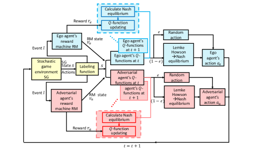
Figure 2: Flowchart of QRM-SG. Following the motivational example, blue indicates the elements related to the ego agent and red indicates the elements related to the adversarial agent.

QRM-SG is guaranteed to converge to best-response strategies in the limit, as stated in the following theorem and proven in the supplementary materials.

Assumption 1.

Every state $s\in S$, RM states $v_{\mathfrak{e}}\in V_{\mathfrak{e}},v_{\mathfrak{a}}\in V_{\mathfrak{a}}$, and actions $a_{\mathfrak{e}}\in A_{\mathfrak{e}},a_{\mathfrak{a}}\in A_{\mathfrak{a}}$, are visited infinitely often when the number of episodes goes to infinity.

Assumption 2.

The learning rate $\alpha_{t}$ satisfies the following conditions for all $t$:

1. $0<\alpha_{t}<1,\sum_{t=0}^{\infty}\alpha_{t}(s,v_{\mathfrak{e}},v_{\mathfrak{a}},a_{\mathfrak{e}},a_{\mathfrak{a}})=\infty,\sum_{t=0}^{\infty}[\alpha_{t}(s,v_{\mathfrak{e}},v_{\mathfrak{a}},a_{\mathfrak{e}},a_{\mathfrak{a}})]^{2}<\infty$, and the latter two hold uniformly and with probability 1.

2. $\alpha_{t}(s,v_{\mathfrak{e}},v_{\mathfrak{a}},a_{\mathfrak{e}},a_{\mathfrak{a}})=0$ if $(s,v_{\mathfrak{e}},v_{\mathfrak{a}},a_{\mathfrak{e}},a_{\mathfrak{a}})\neq(s^{t},v_{\mathfrak{e}}^{t},v_{\mathfrak{a}}^{t},a_{\mathfrak{e}}^{t},a_{\mathfrak{a}}^{t}).$

Assumptions 1 and 2 are standard assumptions and similar to those in Q-learning [34]. Condition 2 in Assumption 2 requires that at each step, only the Q-function elements related to the current state, RM state, and actions are updated.

Assumption 3.

One of the following conditions holds during learning.

1. Every stage game $(q_{\mathfrak{e}\mathfrak{i}}(s,v_{\mathfrak{e}},v_{\mathfrak{a}}),q_{\mathfrak{a}\mathfrak{i}}(s,v_{\mathfrak{e}},v_{\mathfrak{a}}))$, $\mathfrak{i}\in\{\mathfrak{e},\mathfrak{a}\}$, for all $t,s,v_{\mathfrak{e}},$ and $v_{\mathfrak{a}}$, has a global optimal point ($\tilde{\pi}_{\mathfrak{e}\mathfrak{i}},\tilde{\pi}_{\mathfrak{a}\mathfrak{i}}$), (i.e., $\tilde{\pi}_{\mathfrak{j}\mathfrak{i}}q_{\mathfrak{j}\mathfrak{i}}\geq\tilde{\pi}^{\prime}_{\mathfrak{j}\mathfrak{i}}q_{\mathfrak{j}\mathfrak{i}}$ for any $\tilde{\pi}^{\prime}_{\mathfrak{j}\mathfrak{i}},$ $\mathfrak{j}\in\{\mathfrak{e},\mathfrak{a}\}$) and agents’ rewards in this equilibrium are used to update their Q-functions.

2. Every stage game ($q_{\mathfrak{e}\mathfrak{i}}(s,v_{\mathfrak{e}},v_{\mathfrak{a}}),q_{\mathfrak{a}\mathfrak{i}}(s,v_{\mathfrak{e}},v_{\mathfrak{a}})$), $\mathfrak{i}\in\{\mathfrak{e},\mathfrak{a}\}$, for all $t,s,v_{\mathfrak{e}},$ and $v_{\mathfrak{a}}$, has a saddle point ($\tilde{\pi}_{\mathfrak{e}\mathfrak{i}},\tilde{\pi}_{\mathfrak{a}\mathfrak{i}}$), (i.e., $\tilde{\pi}_{\mathfrak{j}\mathfrak{i}}\tilde{\pi}_{-\mathfrak{j}\mathfrak{i}}q_{\mathfrak{j}\mathfrak{i}}\geq\tilde{\pi}^{\prime}_{\mathfrak{j}\mathfrak{i}}\tilde{\pi}_{-\mathfrak{j}\mathfrak{i}}q_{\mathfrak{j}\mathfrak{i}}$ for any $\tilde{\pi}^{\prime}_{\mathfrak{j}\mathfrak{i}}$, $\tilde{\pi}_{\mathfrak{j}\mathfrak{i}}\tilde{\pi}_{-\mathfrak{j}\mathfrak{i}}q_{\mathfrak{j}\mathfrak{i}}\leq\tilde{\pi}_{\mathfrak{j}\mathfrak{i}}\tilde{\pi}^{\prime}_{-\mathfrak{j}\mathfrak{i}}q_{\mathfrak{j}\mathfrak{i}}$ for any $\tilde{\pi}^{\prime}_{-\mathfrak{j}\mathfrak{i}}$, $\mathfrak{j}\in\{\mathfrak{e},\mathfrak{a}\}$), and agents’ rewards in this equilibrium are used to update their Q-functions.

In Assumption 3, $\tilde{\pi}_{\mathfrak{j}\mathfrak{i}}$ denotes the strategy of agent $\mathfrak{j}$ at either the global optimal point or the saddle point, given the Q-functions learned by agent $\mathfrak{i}$. $\tilde{\pi}_{-\mathfrak{j}\mathfrak{i}}$ is the strategy of the agent other than agent $\mathfrak{j}$, i.e., $\tilde{\pi}_{-\mathfrak{e}\mathfrak{i}}=\tilde{\pi}_{\mathfrak{a}\mathfrak{i}},\tilde{\pi}_{-\mathfrak{a}\mathfrak{i}}=\tilde{\pi}_{\mathfrak{e}\mathfrak{i}}.$ Assumption 3 requires that the stage game at each time step has either a global optimal point or a saddle point.

Theorem 1.

Under Assumptions 1, 2 and 3, the sequence $q_{\mathfrak{i}t}=(q_{\mathfrak{e}\mathfrak{i}}^{t},q_{\mathfrak{a}\mathfrak{i}}^{t})$ at time $t$, $\mathfrak{i}\in\{\mathfrak{e},\mathfrak{a}\}$ updated by

$$q_{\mathfrak{j}\mathfrak{i}}^{t+1}(s,v_{\mathfrak{e}},v_{\mathfrak{a}},a_{\mathfrak{e}},a_{\mathfrak{a}})=(1-\alpha_{t})q_{\mathfrak{j}\mathfrak{i}}^{t}(s,v_{\mathfrak{e}},v_{\mathfrak{a}},a_{\mathfrak{e}},a_{\mathfrak{a}})+\alpha_{t}\big{(}r_{\mathfrak{j},t}+\gamma\pi_{\mathfrak{e}\mathfrak{i}}(\cdot|s^{\prime},v^{\prime}_{\mathfrak{e}},v^{\prime}_{\mathfrak{a}})\pi_{\mathfrak{a}\mathfrak{i}}(\cdot|s^{\prime},v^{\prime}_{\mathfrak{e}},v^{\prime}_{\mathfrak{a}})q_{\mathfrak{j}\mathfrak{i}}^{t}(s^{\prime},v^{\prime}_{\mathfrak{e}},v^{\prime}_{\mathfrak{a}})\big{)}$$ (5)

for $\mathfrak{j}\in\{\mathfrak{e},\mathfrak{a}\}$, where $(\pi_{\mathfrak{e}\mathfrak{i}}(\cdot|s^{\prime},v^{\prime}_{\mathfrak{e}},v^{\prime}_{\mathfrak{a}}),\pi_{\mathfrak{a}\mathfrak{i}}(\cdot|s^{\prime},v^{\prime}_{\mathfrak{e}},v^{\prime}_{\mathfrak{a}}))$ is the appropriate type of Nash equilibrium solution for the stage game $(q_{\mathfrak{e}\mathfrak{i}}^{t}(s^{\prime},v^{\prime}_{\mathfrak{e}},v^{\prime}_{\mathfrak{a}}),q_{\mathfrak{a}\mathfrak{i}}^{t}(s^{\prime},v^{\prime}_{\mathfrak{e}},v^{\prime}_{\mathfrak{a}}))$, converges to the Q-functions at a Nash equilibrium $(q^{\ast}_{\mathfrak{e}\mathfrak{i}},q^{\ast}_{\mathfrak{a}\mathfrak{i}})$.

Note that $(\pi_{\mathfrak{e}\mathfrak{i}}(\cdot|s^{\prime},v^{\prime}_{\mathfrak{e}},v^{\prime}_{\mathfrak{a}}),\pi_{\mathfrak{a}\mathfrak{i}}(\cdot|s^{\prime},v^{\prime}_{\mathfrak{e}},v^{\prime}_{\mathfrak{a}}))$ is the appropriate type of Nash equilibrium solution if the strategy corresponds to the global optimal point or the saddle point for the stage game $(q_{\mathfrak{e}\mathfrak{i}}^{t}(s^{\prime},v^{\prime}_{\mathfrak{e}},v^{\prime}_{\mathfrak{a}}),q_{\mathfrak{a}\mathfrak{i}}^{t}(s^{\prime},v^{\prime}_{\mathfrak{e}},v^{\prime}_{\mathfrak{a}}))$. $q^{\ast}_{\mathfrak{i}\mathfrak{j}}$ is the Q-function at a Nash equilibrium for agent $\mathfrak{i}$ and learned by agent $\mathfrak{j}$.

6 Experiments

In this section, we evaluate the effectiveness of the proposed QRM-SG method in three case studies. We compare QRM-SG with following baseline methods:

• Nash-Q: we perform Nash Q-learning algorithm developed in [4] and the agents’ locations are taken as the state.
  

• Nash-QAS (Nash Q-learning in augmented state space): to have more information on high-level events, we include an extra binary vector in the state representing whether each event has been encountered or not.
  

• MADDPG-SG (multi-agent deep deterministic policy gradient with state of the stochastic game): we adopt one of the state-of-the-art MARL baselines — MADDPG algorithm developed in [5] — and include the agents’ locations as the state.
  

• MADDPG-AS (multi-agent deep deterministic policy gradient in augmented state space): similar to Nash-QAS, we include an extra binary vector in the state to represent high-level information for MADDPG [5].

In each case study, each agent is given a task with sparse rewards to achieve, which can be specified as a reward machine. Each agent receives a reward of one if and only if the task is completed. We have two agents in a 6$\times$6 grid world for three case studies, as shown in Figure 3. Following the notations in the motivational example, we use the blue color to indicate the locations corresponding to the ego agent and the red color for the adversarial agent. The power bases are represented by circles and starting locations are represented by triangles. At each time step, each agent can select from: {up, down, left, right}. Each action has a slip rate of 0.5% and $\epsilon$ is set to 0.25.

Figure 3: The grid world for case studies. In Case Study I and II, the adversarial agent starts from location ‘a’. In Case Study III, the adversarial agent starts from location ‘a’ or ‘b’.

(a) Case study I.

(b) Case studies II and III.

Figure 4: The reward machines used in the case studies. In each case study, the reward machine of each agent has the same structure, only the reward differs. Hence, we present the rewards for agent in blue, and the rewards for agent in red. The reward is sparse (zero for both agents when not specified on a transition). Omitted transitions are self-looping transitions with reward 0.

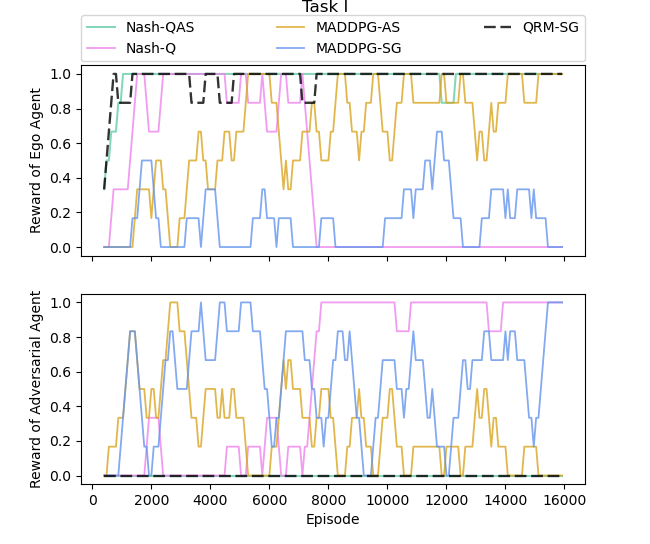
(a) Case study I.

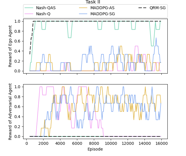
(b) Case study II.

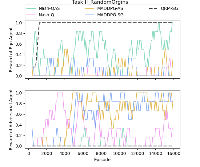
(c) Case study III.

Figure 5: Cumulative reward comparison for each case study. Smoothed plot with a rolling window of size 6. QRM-SG is the proposed method.

The first case study is designed as an ’appetizer’ to test QRM-SG. Then, we make the ego agent’s task more demanding in the second and third case studies. Randomnesses in the starting locations of the adversarial agent are included in the third case study. We define that one agent is captured by the other agent when the distance between two agents is smaller than 2. Each agent is considered to complete the task after capturing the other agent. Only when an agent is the more powerful of the two agents, it has the capability to capture the other agent. We set different conditions for the ego agent to be the more powerful in different case studies. The tasks for agents to complete are specified as reward machines, which are demonstrated in Figure 4. The adversarial agent is given the same task in three case studies, which requires it to be the more powerful by reaching its power base ( ) and then capture the ego agent ( ). In Case Study I, the ego agent is required to first reach its own power base ( ), then destroy/reach the adversarial agent’s power base ( ) to be the more powerful, and capture the adversarial agent afterward ( ). In Case Study II, the required sequential events for the ego agent to be powerful are: reaching its power base ( ), reaching the adversarial agent’s power base ( ), reaching its power base ( ). These events demonstrate the scenario in that the ego agent first gets energy at its power base, destroys the adversarial agent’s power base using most of its energy, and then gets recharged to capture the adversarial agent. Case Study III is different from Case Study II in that the adversarial agent randomly samples the starting location from 2 possible locations. In all case studies, we define that after the adversarial agent arrives at its power base, the ego agent has to reach its own power base again to be able to destroy the adversarial agent’s power base. After a power base is destroyed, the corresponding agent is not possible to be more powerful.

To better analyze the results, each case study is designed to have best-response strategies for agents. The ego agent is expected to complete the required sequence of events to be the more powerful agent, capture the adversarial agent, and complete the task resulting in a cumulative reward of 1. As the adversarial agent is far away from its power base, its power base would be destroyed by the ego agent before it arrives at a Nash equilibrium. Thus, the adversarial agent would fail to complete its task. The learning processes of each agent in three case studies are plotted in Figures 5(a), 5(b) and 5(c). Every 80 episodes, we stop learning, test the algorithms’ performance, and save the cumulative rewards of each agent. In Case Study I, QRM-SG finds the Nash equilibrium in around 7500 episodes. Nash-QAS finds the Nash equilibrium after 12000 episodes, which indicates that using the augmented state can be sufficient for the ego agent to learn to complete the task. When learning by Nash-Q, the adversarial agent completes the task. The reason can be that the task for the adversarial agent is much easier. MADDPG-SG and MADDPG-AS do not converge within 16000 episodes. In MADDPG-SG, the ego agent needs more episodes for completing the task compared to MADDPG-AS. One possible reason is that MADDPG-AS perceives more information represented in the augmented state space. In Case Study II, the policies of agents reach the Nash equilibrium after around 1000 episodes utilizing QRM-SG, while baselines fail to converge to the Nash equilibrium. In Case Study III, QRM-SG finds the Nash equilibrium in around 1500 episodes, while baselines have difficulty converging to the Nash equilibrium. The ego agent learned by Nash-QAS receives a higher reward than other baselines. The ego agent learned by other baselines rarely finishes the task. From the results of the three case studies, QRM-SG outperforms the four baseline methods, where the ego agent can accomplish the task at a Nash equilibrium in several thousand episodes.

An analysis of the effect of $\epsilon$ on the performance of QRM-SG is available in the supplementary materials. Additionally, an extensive evaluation of QRM-SG on a 12$\times$12 grid world is conducted in the supplementary materials.

7 Conclusions

In this paper, we introduce the utilization of reward machines to expose the structure of non-Markovian reward functions for the learning agents in two-agent general-sum stochastic games. Each task is specified by a reward machine. We propose QRM-SG as a variant of Q-learning for the setting of stochastic games and integrated with reward machines to learn best-response strategies at a Nash equilibrium for each agent. We prove that QRM-SG converges to Q-functions at a Nash equilibrium under certain conditions. Three case studies are conducted to evaluate the performance of QRM-SG.

This paper opens the door for using reward machines in stochastic games. First, one immediate extension is to jointly learn reward machines and best-response strategies during RL. Second, extending the methodology to general-sum stochastic games with more agents is worth further investigation. Finally, the same methodology can be readily applied to other forms of RL, such as model-based RL, or actor-critic methods.

Appendix A Proof of Theorem 1

In the supplementary material, we provide the convergence proof of QRM-SG in Theorem 1. Recall that agent $\mathfrak{i}$ ($\mathfrak{i}\in\{\mathfrak{e},\mathfrak{a}\}$) in QRM-SG maintains the Q-functions of both agents $q_{\mathfrak{i}}=(q_{\mathfrak{e}\mathfrak{i}},q_{\mathfrak{a}\mathfrak{i}})$ in the two-agent stochastic game. Agents aim to find the best-response strategies given their own estimations of the Q-functions of both agents. We prove that $(q_{\mathfrak{e}\mathfrak{i}},q_{\mathfrak{a}\mathfrak{i}})$ converges to the Q-functions at a Nash equilibrium $(q^{\ast}_{\mathfrak{e}},q^{\ast}_{\mathfrak{a}})$ for agent $\mathfrak{i}$. In the supplementary materials, to simplify the notation, we omit the subscript ${\mathfrak{i}}$ (which represents the learning agent $\mathfrak{i}$) in the Q-functions. Each agent is equipped with $q=(q_{\mathfrak{e}},q_{\mathfrak{a}})$ and strategy estimations of both agents $\pi=(\pi_{\mathfrak{e}},\pi_{\mathfrak{a}})$. The proof is based on the following lemma in [35].

Lemma 2.

Assume that $\alpha_{t}$ satisfies Assumption 2 and the mapping $F^{t}:\mathbb{Q}\rightarrow\mathbb{Q}$ satisfies the following condition: there exists a number $0<\beta<1$ and a sequence $\lambda^{t}\geq 0$ converging to zero with probability 1 such that $||F^{t}q-F^{t}q^{\ast}||\leq\beta||q-q^{\ast}||+\lambda^{t}$ for all $q\in\mathbb{Q}$ and $q^{\ast}=\mathbb{E}[F^{t}q^{\ast}]$, then the iteration defined by

$$q^{t+1}=(1-\alpha_{t})q^{t}+\alpha_{t}[F^{t}q^{t}]$$ (6)

converges to $q^{\ast}$ with probability 1.

Q-functions in QRM-SG uses the same updating structure as the iteration equation in Equation 6. Thus, we show the convergence of Q-functions in QRM-SG to the Q-functions at a Nash equilibrium by adapting Equation 6 to QRM-SG. We first define the operator $F^{t}$ in the two-agent stochastic game and then prove $F^{t}$ satisfies the condition in Lemma 2.

For each agent, we have $q=(q_{\mathfrak{e}},q_{\mathfrak{a}})$, where $q\in\mathbb{Q}\text{ and }q_{\mathfrak{j}}\in\mathbb{Q}_{\mathfrak{j}}$ for $\mathfrak{j}={\mathfrak{e}},{\mathfrak{a}}$. Thus, $\mathbb{Q}=\mathbb{Q}_{\mathfrak{e}}\times\mathbb{Q}_{\mathfrak{a}}$. Recall that the Q-functions in QRM-SG are in augmented state space, taking the state of the stochastic game and states of the reward machines as input.

Definition 7.

We define the mapping $F^{t}:\mathbb{Q}\rightarrow\mathbb{Q}$ is on the complete metric space $\mathbb{Q}$ to $\mathbb{Q}$, $F^{t}q=(F^{t}q_{\mathfrak{e}},F^{t}q_{\mathfrak{a}})$, where

$$\text{For }\mathfrak{j}\in\{\mathfrak{e},\mathfrak{a}\},F^{t}q_{\mathfrak{j}}(s,v_{\mathfrak{e}},v_{\mathfrak{a}},a_{\mathfrak{e}},a_{\mathfrak{a}})=r_{\mathfrak{j},t}+\gamma\pi_{\mathfrak{e}}(s^{\prime},v^{\prime}_{\mathfrak{e}},v^{\prime}_{\mathfrak{a}})\pi_{\mathfrak{a}}(s^{\prime},v^{\prime}_{\mathfrak{e}},v^{\prime}_{\mathfrak{a}})q_{\mathfrak{j}}(s^{\prime},v^{\prime}_{\mathfrak{e}},v^{\prime}_{\mathfrak{a}})$$ (7)

where $(s^{\prime},v^{\prime}_{\mathfrak{e}},v^{\prime}_{\mathfrak{a}})$ represents the state and RM states in the next time step, and $(\pi_{\mathfrak{e}}(s^{\prime},v^{\prime}_{\mathfrak{e}},v^{\prime}_{\mathfrak{a}}),\pi_{\mathfrak{a}}(s^{\prime},v^{\prime}_{\mathfrak{e}},v^{\prime}_{\mathfrak{a}}))$ represents a Nash equilibrium solution for the stage game ($q_{\mathfrak{e}}(s^{\prime},v^{\prime}_{\mathfrak{e}},v^{\prime}_{\mathfrak{a}}),q_{\mathfrak{a}}(s^{\prime},v^{\prime}_{\mathfrak{e}},v^{\prime}_{\mathfrak{a}})$). $\pi_{\mathfrak{e}}(s^{\prime},v^{\prime}_{\mathfrak{e}},v^{\prime}_{\mathfrak{a}})\pi_{\mathfrak{a}}(s^{\prime},v^{\prime}_{\mathfrak{e}},v^{\prime}_{\mathfrak{a}})$ denotes the probabilities of all possible combined actions and $q_{\mathfrak{j}}(s^{\prime},v^{\prime}_{\mathfrak{e}},v^{\prime}_{\mathfrak{a}})$ denotes all Q-values of combined actions at state $(s^{\prime},v^{\prime}_{\mathfrak{e}},v^{\prime}_{\mathfrak{a}})$. We note that the product of $\pi_{\mathfrak{e}}(s^{\prime},v^{\prime}_{\mathfrak{e}},v^{\prime}_{\mathfrak{a}})\pi_{\mathfrak{a}}(s^{\prime},v^{\prime}_{\mathfrak{e}},v^{\prime}_{\mathfrak{a}})$ and $q_{\mathfrak{j}}(s^{\prime},v^{\prime}_{\mathfrak{e}},v^{\prime}_{\mathfrak{a}})$ is a scalar.

Recall that in an SG, agent $\mathfrak{j}$ $(\mathfrak{j}\in\{\mathfrak{e},\mathfrak{a}\})$ aims to maximize the expected discounted cumulative reward $\tilde{v}_{\mathfrak{j}}$. In the stage game ($q^{\ast}_{\mathfrak{e}}(s,v_{\mathfrak{e}},v_{\mathfrak{a}}),q^{\ast}_{\mathfrak{a}}(s,v_{\mathfrak{e}},v_{\mathfrak{a}})$), the optimal discounted cumulative reward $\tilde{v}_{\mathfrak{j}}$ can be linked to the rewards when the agents reach a Nash equilibrium based on the following lemma in [36].

Lemma 3.

The following assertions are equivalent:

1. $(\pi^{\ast}_{\mathfrak{e}},\pi^{\ast}_{\mathfrak{a}})$ is a Nash equilibrium point in a stochastic game with rewards ($\tilde{v}_{\mathfrak{e}}(\pi^{\ast}_{\mathfrak{e}},\pi^{\ast}_{\mathfrak{a}}),\tilde{v}_{\mathfrak{a}}(\pi^{\ast}_{\mathfrak{e}},\pi^{\ast}_{\mathfrak{a}})$), where $\tilde{v}_{\mathfrak{j}}(\pi^{\ast}_{\mathfrak{e}},\pi^{\ast}_{\mathfrak{a}})=\big{(}\tilde{v}_{\mathfrak{j}}(s^{1},v^{1}_{\mathfrak{e}},v^{1}_{\mathfrak{a}},\pi^{\ast}_{\mathfrak{e}},\pi^{\ast}_{\mathfrak{a}}),\dots,\tilde{v}_{\mathfrak{j}}(s^{k},v^{k}_{\mathfrak{e}},v^{k}_{\mathfrak{a}},\pi^{\ast}_{\mathfrak{e}},\pi^{\ast}_{\mathfrak{a}})\big{)},\mathfrak{j}\in\{\mathfrak{e},\mathfrak{a}\}$

2. For each $(s,v_{\mathfrak{e}},v_{\mathfrak{a}})\in S\times V_{\mathfrak{e}}\times V_{\mathfrak{a}}$, a Nash equilibrium point $\big{(}\pi^{\ast}_{\mathfrak{e}}(s,v_{\mathfrak{e}},v_{\mathfrak{a}}),\pi^{\ast}_{\mathfrak{a}}(s,v_{\mathfrak{e}},v_{\mathfrak{a}})\big{)}$ in the stage game $\big{(}q^{\ast}_{\mathfrak{e}}(s,v_{\mathfrak{e}},v_{\mathfrak{a}}),q^{\ast}_{\mathfrak{a}}(s,v_{\mathfrak{e}},v_{\mathfrak{a}})\big{)}$ achieves rewards $\big{(}\tilde{v}_{\mathfrak{e}}(s,v_{\mathfrak{e}},v_{\mathfrak{a}},\pi^{\ast}_{\mathfrak{e}},\pi^{\ast}_{\mathfrak{a}}),\tilde{v}_{\mathfrak{a}}(s,v_{\mathfrak{e}},v_{\mathfrak{a}},\pi^{\ast}_{\mathfrak{e}},\pi^{\ast}_{\mathfrak{a}})\big{)}$, where for $\mathfrak{j}\in\{\mathfrak{e},\mathfrak{a}\}$,

   $$q^{\ast}_{\mathfrak{j}}=r_{\mathfrak{j}}+\gamma\sum_{\begin{subarray}{c}s^{\prime}\in S\\ v^{\prime}_{\mathfrak{e}}\in V_{\mathfrak{e}}\\ v^{\prime}_{\mathfrak{a}}\in V_{\mathfrak{a}}\end{subarray}}p(s^{\prime},v^{\prime}_{\mathfrak{e}},v^{\prime}_{\mathfrak{a}}|s,v_{\mathfrak{e}},v_{\mathfrak{a}},a_{\mathfrak{e}},a_{\mathfrak{a}})\tilde{v}_{\mathfrak{j}}(s^{\prime},v^{\prime}_{\mathfrak{e}},v^{\prime}_{\mathfrak{a}},\pi_{\mathfrak{e}}^{\ast},\pi_{\mathfrak{a}}^{\ast})$$ (8)

Lemma 3 demonstrates the relationship between $q^{\ast}_{\mathfrak{j}}$ and $\tilde{v}_{\mathfrak{j}}$, $\tilde{v}_{\mathfrak{j}}(s,v_{\mathfrak{e}},v_{\mathfrak{a}})=\pi^{\ast}_{\mathfrak{e}}(s,v_{\mathfrak{e}},v_{\mathfrak{a}})\pi^{\ast}_{\mathfrak{a}}(s,v_{\mathfrak{e}},v_{\mathfrak{a}})q^{\ast}(s,v_{\mathfrak{e}},v_{\mathfrak{a}})$. With Lemma 3, we can achieve $q^{\ast}=\mathbb{E}[F^{t}q^{\ast}]$ shown as follows.

Lemma 4.

For a two-agent stochastic game, given that $F^{t}$ is defined in Definition 7, $q^{\ast}$ is the Q-functions at a Nash equilibrium, and $q^{\ast}=(q^{\ast}_{\mathfrak{e}},q^{\ast}_{\mathfrak{a}})$, we have $q^{\ast}=\mathbb{E}[F^{t}q^{\ast}]$.

Proof.

In the stage game $\big{(}q^{\ast}_{\mathfrak{e}}(s^{\prime},v^{\prime}_{\mathfrak{e}},v^{\prime}_{\mathfrak{a}}),q^{\ast}_{\mathfrak{a}}(s^{\prime},v^{\prime}_{\mathfrak{e}},v^{\prime}_{\mathfrak{a}})\big{)}$, given the strategies at a Nash equilibrium point $\big{(}\pi^{\ast}_{\mathfrak{e}}(s^{\prime},v^{\prime}_{\mathfrak{e}},v^{\prime}_{\mathfrak{a}}),\\ \pi^{\ast}_{\mathfrak{a}}(s^{\prime},v^{\prime}_{\mathfrak{e}},v^{\prime}_{\mathfrak{a}})\big{)}$ and the reward $\tilde{v}_{\mathfrak{j}}(s^{\prime},v^{\prime}_{\mathfrak{e}},v^{\prime}_{\mathfrak{a}},\pi^{\ast}_{\mathfrak{e}},\pi^{\ast}_{\mathfrak{a}})$ of agent $\mathfrak{j}$ obtained at the Nash equilibrium point, $\tilde{v}_{\mathfrak{j}}(s^{\prime},v^{\prime}_{\mathfrak{e}},v^{\prime}_{\mathfrak{a}},\pi^{\ast}_{\mathfrak{e}},\pi^{\ast}_{\mathfrak{a}})\\ =\pi^{\ast}_{\mathfrak{e}}(s^{\prime},v^{\prime}_{\mathfrak{e}},v^{\prime}_{\mathfrak{a}})\pi^{\ast}_{\mathfrak{a}}(s^{\prime},v^{\prime}_{\mathfrak{e}},v^{\prime}_{\mathfrak{a}})q^{\ast}_{\mathfrak{j}}(s^{\prime},v^{\prime}_{\mathfrak{e}},v^{\prime}_{\mathfrak{a}})$. The reward at a Nash equilibrium point depends on the best-response strategies of both agents. Following Lemma 3, for $\mathfrak{j}\in\{\mathfrak{e},\mathfrak{a}\}$,

$$q^{\ast}_{\mathfrak{j}} =r_{\mathfrak{j}}+\allowbreak\gamma\sum_{\begin{subarray}{c}s^{\prime}\in S\\ v^{\prime}_{\mathfrak{e}}\in V_{\mathfrak{e}}\\ v^{\prime}_{\mathfrak{a}}\in V_{\mathfrak{a}}\end{subarray}}p(s^{\prime},v^{\prime}_{\mathfrak{e}},v^{\prime}_{\mathfrak{a}}|s,v_{\mathfrak{e}},v_{\mathfrak{a}},a_{\mathfrak{e}},a_{\mathfrak{a}})\tilde{v}_{\mathfrak{j}}(s^{\prime},v^{\prime}_{\mathfrak{e}},v^{\prime}_{\mathfrak{a}},\pi_{\mathfrak{e}}^{\ast},\pi_{\mathfrak{a}}^{\ast})$$ (9)

$$=r_{\mathfrak{j}}+\allowbreak\gamma\sum_{\begin{subarray}{c}s^{\prime}\in S\\ v^{\prime}_{\mathfrak{e}}\in V_{\mathfrak{e}}\\ v^{\prime}_{\mathfrak{a}}\in V_{\mathfrak{a}}\end{subarray}}p(s^{\prime},v^{\prime}_{\mathfrak{e}},v^{\prime}_{\mathfrak{a}}|s,v_{\mathfrak{e}},v_{\mathfrak{a}},a_{\mathfrak{e}},a_{\mathfrak{a}})\pi^{\ast}_{\mathfrak{e}}(s^{\prime},v^{\prime}_{\mathfrak{e}},v^{\prime}_{\mathfrak{a}})\pi^{\ast}_{\mathfrak{a}}(s^{\prime},v^{\prime}_{\mathfrak{e}},v^{\prime}_{\mathfrak{a}})q^{\ast}_{\mathfrak{j}}(s^{\prime},v^{\prime}_{\mathfrak{e}},v^{\prime}_{\mathfrak{a}})$$

$$=\sum_{\begin{subarray}{c}s^{\prime}\in S\\ v^{\prime}_{\mathfrak{e}}\in V_{\mathfrak{e}}\\ v^{\prime}_{\mathfrak{a}}\in V_{\mathfrak{a}}\end{subarray}}p(s^{\prime},v^{\prime}_{\mathfrak{e}},v^{\prime}_{\mathfrak{a}}|s,v_{\mathfrak{e}},v_{\mathfrak{a}},a_{\mathfrak{e}},a_{\mathfrak{a}})\big{(}r_{\mathfrak{j}}+\gamma\pi^{\ast}_{\mathfrak{e}}(s^{\prime},v^{\prime}_{\mathfrak{e}},v^{\prime}_{\mathfrak{a}})\pi^{\ast}_{\mathfrak{a}}(s^{\prime},v^{\prime}_{\mathfrak{e}},v^{\prime}_{\mathfrak{a}})q^{\ast}_{\mathfrak{j}}(s^{\prime},v^{\prime}_{\mathfrak{e}},v^{\prime}_{\mathfrak{a}})\big{)}$$

$$=\mathbb{E}[F^{t}q^{\ast}_{\mathfrak{j}}]$$

As $q^{\ast}_{\mathfrak{e}}=\mathbb{E}[F^{t}q^{\ast}_{\mathfrak{e}}]$ and $q^{\ast}_{\mathfrak{a}}=\mathbb{E}[F^{t}q^{\ast}_{\mathfrak{a}}]$, we have $q^{\ast}=\mathbb{E}[F^{t}q^{\ast}]$. ∎

In Assumption 3, we introduce a global optimal point $(\tilde{\pi}_{\mathfrak{e}},\tilde{\pi}_{\mathfrak{a}})$ of the stage game $(q_{\mathfrak{e}}(s,v_{\mathfrak{e}},v_{\mathfrak{a}}),q_{\mathfrak{a}}(s,v_{\mathfrak{e}},v_{\mathfrak{a}}))$, and we have $\tilde{\pi}_{\mathfrak{j}}q_{\mathfrak{j}}\geq\tilde{\pi}^{\prime}_{\mathfrak{j}}q_{\mathfrak{j}}$ for any $\tilde{\pi}^{\prime}_{\mathfrak{j}},$ $\mathfrak{j}\in\{\mathfrak{e},\mathfrak{a}\}$. A global optimal point is a Nash equilibrium and all global optima are equivalent in their values.

Lemma 5.

Let $\tilde{\pi}=(\tilde{\pi}_{\mathfrak{e}},\tilde{\pi}_{\mathfrak{a}})$ and $\acute{\pi}=(\acute{\pi}_{\mathfrak{e}},\acute{\pi}_{\mathfrak{a}})$ denote the global optimal points of the two-agent stage game $(q_{\mathfrak{e}},q_{\mathfrak{a}})$. Then, $\tilde{\pi}q_{\mathfrak{j}}=\acute{\pi}q_{\mathfrak{j}}$, for $\mathfrak{j}\in\{\mathfrak{e},\mathfrak{a}\}$.

Proof.

According to the definition of a global point,

$$\tilde{\pi}_{\mathfrak{j}}q_{\mathfrak{j}}\geq\acute{\pi}_{\mathfrak{j}}q_{\mathfrak{j}}\text{ and }\acute{\pi}_{\mathfrak{j}}q_{\mathfrak{j}}\geq\tilde{\pi}_{\mathfrak{j}}q_{\mathfrak{j}}$$ (10)

Then, the only consistent solution is $\tilde{\pi}_{\mathfrak{j}}q_{\mathfrak{j}}=\acute{\pi}_{\mathfrak{j}}q_{\mathfrak{j}}$ ∎

Similarly, all saddle points introduced in Assumption 3 have equal values.

Lemma 6.

Let $\tilde{\pi}=(\tilde{\pi}_{\mathfrak{e}},\tilde{\pi}_{\mathfrak{a}}$) and $\acute{\pi}=(\acute{\pi}_{\mathfrak{e}},\acute{\pi}_{\mathfrak{a}}$) denote the saddle points of the two-agent stage game ($q_{\mathfrak{e}},q_{\mathfrak{a}}$). Then $\tilde{\pi}q_{\mathfrak{j}}=\acute{\pi}q_{\mathfrak{j}}$, for $\mathfrak{j}\in\{\mathfrak{e},\mathfrak{a}\}$.

Proof.

According to the definition of a saddle point,

$$\tilde{\pi}_{\mathfrak{j}}\tilde{\pi}_{-\mathfrak{j}}q_{\mathfrak{j}}\geq\acute{\pi}_{\mathfrak{j}}\tilde{\pi}_{-\mathfrak{j}}q_{\mathfrak{j}}$$ (11)

$$\acute{\pi}_{\mathfrak{j}}\acute{\pi}_{-\mathfrak{j}}q_{\mathfrak{j}}\leq\acute{\pi}_{\mathfrak{j}}\tilde{\pi}_{-\mathfrak{j}}q_{\mathfrak{j}}$$

Then, we have $\tilde{\pi}_{\mathfrak{j}}\tilde{\pi}_{-\mathfrak{j}}q_{\mathfrak{j}}\geq\acute{\pi}_{\mathfrak{j}}\acute{\pi}_{-\mathfrak{j}}q_{\mathfrak{j}}$. Similarly, we can have $\acute{\pi}_{\mathfrak{j}}\acute{\pi}_{-\mathfrak{j}}q_{\mathfrak{j}}\geq\tilde{\pi}_{\mathfrak{j}}\tilde{\pi}_{-\mathfrak{j}}q_{\mathfrak{j}}$. Then, the only consistent solution is

$$\tilde{\pi}_{\mathfrak{j}}\tilde{\pi}_{-\mathfrak{j}}q_{\mathfrak{j}}=\acute{\pi}_{\mathfrak{j}}\acute{\pi}_{-\mathfrak{j}}q_{\mathfrak{j}}$$ (12)

Thus, we have $\tilde{\pi}q_{\mathfrak{j}}=\acute{\pi}q_{\mathfrak{j}}$. ∎

In Equation 6, the other condition for the convergence of $q$ to $q^{\ast}$ is that $||F^{t}q-F^{t}q^{\ast}||\leq\beta||q-q^{\ast}||+\lambda^{t}$, which requires that $F^{t}$ is a pseudo-contraction operator. $F^{t}$ maps $q\in\mathbb{Q}$ to $q^{\ast}$ when $\lambda=0$. We restrict the stage games to have a global optimal point or a saddle point at a Nash equilibrium as mentioned in Assumption 3. Under such restriction, we prove that $F^{t}$ is a real contraction operator, mapping every two points $q$ and $\acute{q}$ in the space $\mathbb{Q}$ close to each other, as introduced in Lemma 7. As a real contraction operator is a stronger version of the pseudo-contraction operator, the real contraction operator $F^{t}$ satisfies the condition on the contraction property in Equation 6. We first define the distance between two Q-functions.

Definition 8.

For $q,\acute{q}\in\mathbb{Q}$, the distance between Q-functions is defined as

$$||q-\acute{q}||=\max_{\mathfrak{j}\in\{\mathfrak{e},\mathfrak{a}\}}\max_{(s,v_{\mathfrak{e}},v_{\mathfrak{a}})}\max_{a_{\mathfrak{e}},a_{\mathfrak{a}}}||q_{\mathfrak{j}}(s,v_{\mathfrak{e}},v_{\mathfrak{a}})-\acute{q}_{\mathfrak{j}}(s,v_{\mathfrak{e}},v_{\mathfrak{a}})||$$ (13)

Then, we show the operator $F^{t}$ defined in Definition 7 is a contraction mapping operator.

Lemma 7.

$||F^{t}q-F^{t}\acute{q}||\leq\gamma||q-\acute{q}||$ for all $q,\acute{q}\in\mathbb{Q}$, where $F^{t}$ is defined in Definition 7.

Proof.

Given $(\pi_{\mathfrak{e}},\pi_{\mathfrak{a}})$ is the Nash equilibrium strategy for the stage game $(q_{\mathfrak{e}},q_{\mathfrak{a}})$, $(\acute{\pi}_{\mathfrak{e}},\acute{\pi}_{\mathfrak{a}})$ is the Nash equilibrium strategy for the stage game $(\acute{q}_{\mathfrak{e}},\acute{q}_{\mathfrak{a}})$, we have

$$||F^{t}q-F^{t}\acute{q}|| =\max_{\mathfrak{j}}\max_{(s,v_{\mathfrak{e}},v_{\mathfrak{a}})}|\gamma\pi_{\mathfrak{e}}(s,v_{\mathfrak{e}},v_{\mathfrak{a}})\pi_{\mathfrak{a}}(s,v_{\mathfrak{e}},v_{\mathfrak{a}})q_{\mathfrak{j}}(s,v_{\mathfrak{e}},v_{\mathfrak{a}})-\gamma\acute{\pi}_{\mathfrak{e}}(s,v_{\mathfrak{e}},v_{\mathfrak{a}})\acute{\pi}_{\mathfrak{a}}(s,v_{\mathfrak{e}},v_{\mathfrak{a}})\acute{q}_{\mathfrak{j}}(s,v_{\mathfrak{e}},v_{\mathfrak{a}})|$$ (14)

$$=\max_{\mathfrak{j}}\max_{(s,v_{\mathfrak{e}},v_{\mathfrak{a}})}\gamma|\pi_{\mathfrak{e}}(s,v_{\mathfrak{e}},v_{\mathfrak{a}})\pi_{\mathfrak{a}}(s,v_{\mathfrak{e}},v_{\mathfrak{a}})q_{\mathfrak{j}}(s,v_{\mathfrak{e}},v_{\mathfrak{a}})-\acute{\pi}_{\mathfrak{e}}(s,v_{\mathfrak{e}},v_{\mathfrak{a}})\acute{\pi}_{\mathfrak{a}}(s,v_{\mathfrak{e}},v_{\mathfrak{a}})\acute{q}_{\mathfrak{j}}(s,v_{\mathfrak{e}},v_{\mathfrak{a}})|$$

To simplify the notation, we omit the inputs of $\pi\text{ and }\acute{\pi}$. The next step is to show

$$|\pi_{\mathfrak{e}}\pi_{\mathfrak{a}}q_{\mathfrak{j}}(s,v_{\mathfrak{e}},v_{\mathfrak{a}})-\acute{\pi}_{\mathfrak{e}}\acute{\pi}_{\mathfrak{a}}\acute{q}_{\mathfrak{j}}(s,v_{\mathfrak{e}},v_{\mathfrak{a}})|\leq||q(s,v_{\mathfrak{e}},v_{\mathfrak{a}})-\acute{q}(s,v_{\mathfrak{e}},v_{\mathfrak{a}})||$$ (15)

1. Under condition 1 in Assumption 3:

Both $(\pi_{\mathfrak{e}},\pi_{\mathfrak{a}})$ and $(\acute{\pi}_{\mathfrak{e}},\acute{\pi}_{\mathfrak{a}})$ are global optimal points.

If $\pi_{\mathfrak{e}}\pi_{\mathfrak{a}}q_{\mathfrak{j}}(s,v_{\mathfrak{e}},v_{\mathfrak{a}})\geq\acute{\pi}_{\mathfrak{e}}\acute{\pi}_{\mathfrak{a}}\acute{q}_{\mathfrak{j}}(s,v_{\mathfrak{e}},v_{\mathfrak{a}})$, we have

$$\pi_{\mathfrak{e}}\pi_{\mathfrak{a}}q_{\mathfrak{j}}(s,v_{\mathfrak{e}},v_{\mathfrak{a}})-\acute{\pi}_{\mathfrak{e}}\acute{\pi}_{\mathfrak{a}}\acute{q}_{\mathfrak{j}}(s,v_{\mathfrak{e}},v_{\mathfrak{a}})$$ (16)

$$\leq \pi_{\mathfrak{e}}\pi_{\mathfrak{a}}q_{\mathfrak{j}}(s,v_{\mathfrak{e}},v_{\mathfrak{a}})-\pi_{\mathfrak{e}}\pi_{\mathfrak{a}}\acute{q}_{\mathfrak{j}}(s,v_{\mathfrak{e}},v_{\mathfrak{a}})$$

$$= \sum_{a_{\mathfrak{e}},a_{\mathfrak{a}}}\pi_{\mathfrak{e}}(a_{\mathfrak{e}})\pi_{\mathfrak{a}}(a_{\mathfrak{a}})(q_{\mathfrak{j}}(s,v_{\mathfrak{e}},v_{\mathfrak{a}},a_{\mathfrak{e}},a_{\mathfrak{a}})-\acute{q}_{\mathfrak{j}}(s,v_{\mathfrak{e}},v_{\mathfrak{a}},a_{\mathfrak{e}},a_{\mathfrak{a}}))$$

$$\leq \sum_{a_{\mathfrak{e}},a_{\mathfrak{a}}}\pi_{\mathfrak{e}}(a_{\mathfrak{e}})\pi_{\mathfrak{a}}(a_{\mathfrak{a}})||q_{\mathfrak{j}}(s,v_{\mathfrak{e}},v_{\mathfrak{a}})-\acute{q}_{\mathfrak{j}}(s,v_{\mathfrak{e}},v_{\mathfrak{a}})||$$

$$\leq ||q_{\mathfrak{j}}(s,v_{\mathfrak{e}},v_{\mathfrak{a}})-\acute{q}_{\mathfrak{j}}(s,v_{\mathfrak{e}},v_{\mathfrak{a}})||$$

The first inequality derives from the property of the global point that $\acute{\pi}_{\mathfrak{e}}\acute{\pi}_{\mathfrak{a}}\acute{q}_{\mathfrak{j}}(s,v_{\mathfrak{e}},v_{\mathfrak{a}})\geq\pi_{\mathfrak{e}}\pi_{\mathfrak{a}}\acute{q}_{\mathfrak{j}}(s,v_{\mathfrak{e}},v_{\mathfrak{a}})$. The second inequality is based on $||q_{\mathfrak{j}}(s,v_{\mathfrak{e}},v_{\mathfrak{a}})-\acute{q}_{\mathfrak{j}}(s,v_{\mathfrak{e}},v_{\mathfrak{a}})||=\max_{a_{\mathfrak{e}},a_{\mathfrak{a}}}|q_{\mathfrak{j}}(s,v_{\mathfrak{e}},v_{\mathfrak{a}},a_{\mathfrak{e}},a_{\mathfrak{a}})-\acute{q}_{\mathfrak{j}}(s,v_{\mathfrak{e}},v_{\mathfrak{a}},a_{\mathfrak{e}},a_{\mathfrak{a}})|$.

If $\pi_{\mathfrak{e}}\pi_{\mathfrak{a}}q_{\mathfrak{j}}(s,v_{\mathfrak{e}},v_{\mathfrak{a}})\leq\acute{\pi}_{\mathfrak{e}}\acute{\pi}_{\mathfrak{a}}\acute{q}_{\mathfrak{j}}(s,v_{\mathfrak{e}},v_{\mathfrak{a}})$, we have

$$\acute{\pi}_{\mathfrak{e}}\acute{\pi}_{\mathfrak{a}}\acute{q}_{\mathfrak{j}}(s,v_{\mathfrak{e}},v_{\mathfrak{a}})-\pi_{\mathfrak{e}}\pi_{\mathfrak{a}}q_{\mathfrak{j}}(s,v_{\mathfrak{e}},v_{\mathfrak{a}})\leq\acute{\pi}_{\mathfrak{e}}\acute{\pi}_{\mathfrak{a}}\acute{q}_{\mathfrak{j}}(s,v_{\mathfrak{e}},v_{\mathfrak{a}})-\acute{\pi}_{\mathfrak{e}}\acute{\pi}_{\mathfrak{a}}q_{\mathfrak{j}}(s,v_{\mathfrak{e}},v_{\mathfrak{a}})$$ (17)

and the rest of the proof is similar to the above.

2. Under condition 2 in Assumption 3:

Both $(\pi_{\mathfrak{e}},\pi_{\mathfrak{a}})$ and $(\acute{\pi}_{\mathfrak{e}},\acute{\pi}_{\mathfrak{a}})$ are saddle points.

If $\pi_{\mathfrak{e}}\pi_{\mathfrak{a}}q_{\mathfrak{j}}(s,v_{\mathfrak{e}},v_{\mathfrak{a}})\geq\acute{\pi}_{\mathfrak{e}}\acute{\pi}_{\mathfrak{a}}\acute{q}_{\mathfrak{j}}(s,v_{\mathfrak{e}},v_{\mathfrak{a}})$, we have

$$\pi_{\mathfrak{e}}\pi_{\mathfrak{a}}q_{\mathfrak{j}}(s,v_{\mathfrak{e}},v_{\mathfrak{a}})-\acute{\pi}_{\mathfrak{e}}\acute{\pi}_{\mathfrak{a}}\acute{q}_{\mathfrak{j}}(s,v_{\mathfrak{e}},v_{\mathfrak{a}})$$ (18)

$$\leq\pi_{\mathfrak{e}}\pi_{\mathfrak{a}}q_{\mathfrak{j}}(s,v_{\mathfrak{e}},v_{\mathfrak{a}})-\pi_{\mathfrak{e}}\acute{\pi}_{\mathfrak{a}}\acute{q}_{\mathfrak{j}}(s,v_{\mathfrak{e}},v_{\mathfrak{a}})$$

$$\leq\pi_{\mathfrak{e}}\acute{\pi}_{\mathfrak{a}}q_{\mathfrak{j}}(s,v_{\mathfrak{e}},v_{\mathfrak{a}})-\pi_{\mathfrak{e}}\acute{\pi}_{\mathfrak{a}}\acute{q}_{\mathfrak{j}}(s,v_{\mathfrak{e}},v_{\mathfrak{a}})$$

$$\leq||q_{\mathfrak{j}}(s,v_{\mathfrak{e}},v_{\mathfrak{a}})-\acute{q}_{\mathfrak{j}}(s,v_{\mathfrak{e}},v_{\mathfrak{a}})||$$

The inequalities are based on the properties of saddle points, which are mentioned in Assumption 3.

If $\pi_{\mathfrak{e}}\pi_{\mathfrak{a}}q_{\mathfrak{j}}(s,v_{\mathfrak{e}},v_{\mathfrak{a}})\leq\acute{\pi}_{\mathfrak{e}}\acute{\pi}_{\mathfrak{a}}\acute{q}_{\mathfrak{j}}(s,v_{\mathfrak{e}},v_{\mathfrak{a}})$, the proof is similar to the above.

Thus,

$$||F^{t}q-F^{t}\acute{q}|| =\max_{\mathfrak{j}}\max_{(s,v_{\mathfrak{e}},v_{\mathfrak{a}})}\gamma|\pi_{\mathfrak{e}}(s,v_{\mathfrak{e}},v_{\mathfrak{a}})\pi_{\mathfrak{a}}(s,v_{\mathfrak{e}},v_{\mathfrak{a}})q_{\mathfrak{j}}(s,v_{\mathfrak{e}},v_{\mathfrak{a}})-\acute{\pi}_{\mathfrak{e}}(s,v_{\mathfrak{e}},v_{\mathfrak{a}})\acute{\pi}_{\mathfrak{a}}(s,v_{\mathfrak{e}},v_{\mathfrak{a}})\acute{q}_{\mathfrak{j}}(s,v_{\mathfrak{e}},v_{\mathfrak{a}})|$$ (19)

$$\leq\max_{\mathfrak{j}}\max_{(s,v_{\mathfrak{e}},v_{\mathfrak{a}})}\gamma||q_{\mathfrak{j}}(s,v_{\mathfrak{e}},v_{\mathfrak{a}})-\acute{q}_{\mathfrak{j}}(s,v_{\mathfrak{e}},v_{\mathfrak{a}})||$$

$$\leq\gamma||q-\acute{q}||$$

∎

Based on Lemma 7 and Lemma 4, the operator $F^{t}$ defined for two-agent stochastic game in Definition 7 satisfies the condition for convergence in Lemma 2. Moreover, the updating function of Q-functions in QRM-SG uses the same updating method in Equation 6. Thus, we apply Equation 6 to QRM-SG and achieve Theorem 1 that Q-functions in QRM-SG converge to Q-functions at a Nash equilibrium under certain conditions.

Appendix B Effect of $\epsilon$ on QRM-SG

When using the $\epsilon$-greedy policy, $\epsilon$ determines the probability of taking a random action at each step during training, which affects the balance between exploration and exploitation and would further affect the learning speed [37, 38]. To study the effect of $\epsilon$ on QRM-SG, we compare the performance of QRM-SG with varying $\epsilon$ values to learn the task in Case Study I, including $\epsilon=0.05$, $\epsilon=0.25$ (which is adopted in Section 6), $\epsilon=0.90$, and $\epsilon=0.90$ decaying with $\epsilon\times 0.9986$ until $\epsilon$ reaches 0.05 (which is adopted in  [39]).

We evaluate the performance of QRM-SG with different $\epsilon$ every 80 episodes during training, and Figure 6 plots the cumulative rewards of each agent during the evaluations. We note that $\epsilon$ is set to 0 during the evaluations. When using QRM-SG with $\epsilon$ of 0.05 or 0.90, the ego agent starts to complete the task after around 2000 episodes, significantly more training episodes compared to QRM-SG with $\epsilon$ of 0.25 or decaying $\epsilon$. The reason is that $\epsilon$ with a large value focuses on exploring the environment to collect data about different actions and their outcomes, whereas $\epsilon$ with a small value focuses on actions that have previously resulted in higher rewards. In this case study, $\epsilon$ of 0.25 strikes a balance between exploration and exploitation, allowing the agent to efficiently learn the complex task.

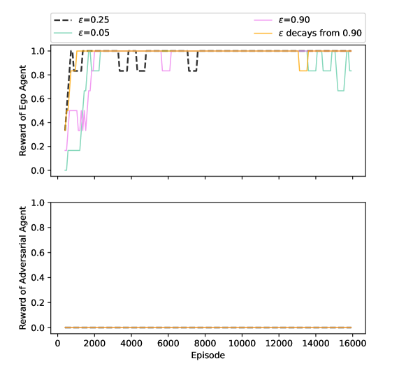
Figure 6: Cumulative reward comparison for learning the task introduced in Case Study I using QRM-SG with varying $\epsilon$. Smoothed plot with a rolling window of size 6. The adversarial agent receives a cumulative reward of 0 with all $\epsilon$ values.

Appendix C Evaluation of QRM-SG on a 12$\times$12 Grid World

To further evaluate the performance of QRM-SG, we generalize QRM-SG to learn the task introduced in Case Study I in a 12$\times$12 grid world. The grid world size aligns with the case studies in other existing research papers, such as the 9$\times$12 office world scenario in [31] and 15$\times$15 grid world in [40]. As shown in Figure 7, the adversarial agent is far away from its power base, thus it is expected to fail to complete its own task, whereas the ego agent is expected to complete its own task. Figure 8 shows the learning process of each agent. Similar to the case studies in Section 6, every 80 episodes, we stop learning, test the algorithm’s performance, and save the cumulative rewards of each agent. The ego agent starts to complete the task after around 7000 episodes and QRM-SG finds the Nash equilibrium in around 21000 episodes.

Figure 7: The 12$\times$12 grid world for scalability analysis of QRM-SG. Locations and denote the power bases of the ego agent and adversarial agent, respectively. and indicate the starting locations of the ego agent and adversarial agent, respectively.

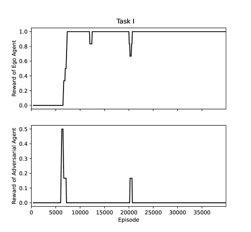
Figure 8: Cumulative reward of learning the task introduced in Case Study I in the 12$\times$12 grid world using QRM-SG. Smoothed plot with a rolling window of size 6.

References

- [1] L. Buşoniu, R. Babuška, and B. D. Schutter, “Multi-agent reinforcement learning: An overview,” in Innovations in Multi-Agent Systems and Applications - 1. Springer Berlin Heidelberg, 2010, pp. 183–221. [Online]. Available: https://doi.org/10.1007/978-3-642-14435-6_7
- [2] R. T. Icarte, T. Klassen, R. Valenzano, and S. McIlraith, “Using reward machines for high-level task specification and decomposition in reinforcement learning,” in International Conference on Machine Learning. PMLR, 2018, pp. 2107–2116.
- [3] C. E. Lemke and J. T. Howson, Jr, “Equilibrium points of bimatrix games,” Journal of the Society for industrial and Applied Mathematics, vol. 12, no. 2, pp. 413–423, 1964.
- [4] J. Hu and M. P. Wellman, “Nash q-learning for general-sum stochastic games,” Journal of machine learning research, vol. 4, no. Nov, pp. 1039–1069, 2003.
- [5] R. Lowe, Y. I. Wu, A. Tamar, J. Harb, O. Pieter Abbeel, and I. Mordatch, “Multi-agent actor-critic for mixed cooperative-competitive environments,” Advances in neural information processing systems, vol. 30, 2017.
- [6] K. Zhang, Z. Yang, H. Liu, T. Zhang, and T. Basar, “Fully decentralized multi-agent reinforcement learning with networked agents,” in International Conference on Machine Learning. PMLR, 2018, pp. 5872–5881.
- [7] G. Palmer, K. Tuyls, D. Bloembergen, and R. Savani, “Lenient multi-agent deep reinforcement learning,” arXiv preprint arXiv:1707.04402, 2017.
- [8] J. Foerster, N. Nardelli, G. Farquhar, T. Afouras, P. H. Torr, P. Kohli, and S. Whiteson, “Stabilising experience replay for deep multi-agent reinforcement learning,” in International conference on machine learning. PMLR, 2017, pp. 1146–1155.
- [9] S. Omidshafiei, J. Pazis, C. Amato, J. P. How, and J. Vian, “Deep decentralized multi-task multi-agent reinforcement learning under partial observability,” in International Conference on Machine Learning. PMLR, 2017, pp. 2681–2690.
- [10] J. K. Gupta, M. Egorov, and M. Kochenderfer, “Cooperative multi-agent control using deep reinforcement learning,” in International conference on autonomous agents and multiagent systems. Springer, 2017, pp. 66–83.
- [11] J. Foerster, G. Farquhar, T. Afouras, N. Nardelli, and S. Whiteson, “Counterfactual multi-agent policy gradients,” in Proceedings of the AAAI conference on artificial intelligence, vol. 32, no. 1, 2018.
- [12] P. Sunehag, G. Lever, A. Gruslys, W. M. Czarnecki, V. Zambaldi, M. Jaderberg, M. Lanctot, N. Sonnerat, J. Z. Leibo, K. Tuyls et al., “Value-decomposition networks for cooperative multi-agent learning,” arXiv preprint arXiv:1706.05296, 2017.
- [13] T. Rashid, M. Samvelyan, C. Schroeder, G. Farquhar, J. Foerster, and S. Whiteson, “Qmix: Monotonic value function factorisation for deep multi-agent reinforcement learning,” in International conference on machine learning. PMLR, 2018, pp. 4295–4304.
- [14] X. Zhang, K. Zhang, E. Miehling, and T. Basar, “Non-cooperative inverse reinforcement learning,” in Advances in Neural Information Processing Systems, H. Wallach, H. Larochelle, A. Beygelzimer, F. d'Alché-Buc, E. Fox, and R. Garnett, Eds., vol. 32. Curran Associates, Inc., 2019. [Online]. Available: https://proceedings.neurips.cc/paper/2019/file/56bd37d3a2fda0f2f41925019c81011d-Paper.pdf
- [15] X. Lin, S. C. Adams, and P. A. Beling, “Multi-agent inverse reinforcement learning for certain general-sum stochastic games,” Journal of Artificial Intelligence Research, vol. 66, pp. 473–502, 2019.
- [16] T. Zhang, Q. Ye, J. Bian, G. Xie, and T.-Y. Liu, “Mfvfd: A multi-agent q-learning approach to cooperative and non-cooperative tasks.” in IJCAI, 2021, pp. 500–506.
- [17] D. H. Mguni, Y. Wu, Y. Du, Y. Yang, Z. Wang, M. Li, Y. Wen, J. Jennings, and J. Wang, “Learning in nonzero-sum stochastic games with potentials,” in Proceedings of the 38th International Conference on Machine Learning, ser. Proceedings of Machine Learning Research, M. Meila and T. Zhang, Eds., vol. 139. PMLR, 18–24 Jul 2021, pp. 7688–7699. [Online]. Available: https://proceedings.mlr.press/v139/mguni21a.html
- [18] M. Hasanbeig, N. Y. Jeppu, A. Abate, T. Melham, and D. Kroening, “Deepsynth: Automata synthesis for automatic task segmentation in deep reinforcement learning,” in Proceedings of the AAAI Conference on Artificial Intelligence, vol. 35, no. 9, 2021, pp. 7647–7656.
- [19] Z. Xu, I. Gavran, Y. Ahmad, R. Majumdar, D. Neider, U. Topcu, and B. Wu, “Joint inference of reward machines and policies for reinforcement learning,” in Proceedings of the International Conference on Automated Planning and Scheduling, vol. 30, 2020, pp. 590–598.
- [20] R. Toro Icarte, E. Waldie, T. Klassen, R. Valenzano, M. Castro, and S. McIlraith, “Learning reward machines for partially observable reinforcement learning,” Advances in neural information processing systems, vol. 32, 2019.
- [21] G. Rens, J.-F. Raskin, R. Reynouad, and G. Marra, “Online learning of non-markovian reward models,” arXiv preprint arXiv:2009.12600, 2020.
- [22] Z. Xu, B. Wu, A. Ojha, D. Neider, and U. Topcu, “Active finite reward automaton inference and reinforcement learning using queries and counterexamples,” in International Cross-Domain Conference for Machine Learning and Knowledge Extraction. Springer, 2021, pp. 115–135.
- [23] G. Rens and J.-F. Raskin, “Learning non-markovian reward models in mdps,” arXiv preprint arXiv:2001.09293, 2020.
- [24] D. Neider, J.-R. Gaglione, I. Gavran, U. Topcu, B. Wu, and Z. Xu, “Advice-guided reinforcement learning in a non-markovian environment,” in Proceedings of the AAAI Conference on Artificial Intelligence, vol. 35, no. 10, 2021, pp. 9073–9080.
- [25] G. De Giacomo, L. Iocchi, M. Favorito, and F. Patrizi, “Restraining bolts for reinforcement learning agents,” in Proceedings of the AAAI Conference on Artificial Intelligence, vol. 34, no. 09, 2020, pp. 13 659–13 662.
- [26] G. De Giacomo, M. Favorito, L. Iocchi, F. Patrizi, and A. Ronca, “Temporal logic monitoring rewards via transducers,” in Proceedings of the International Conference on Principles of Knowledge Representation and Reasoning, vol. 17, no. 1, 2020, pp. 860–870.
- [27] D. Muniraj, K. G. Vamvoudakis, and M. Farhood, “Enforcing signal temporal logic specifications in multi-agent adversarial environments: A deep q-learning approach,” in 2018 IEEE Conference on Decision and Control (CDC), 2018, pp. 4141–4146.
- [28] B. G. León and F. Belardinelli, “Extended markov games to learn multiple tasks in multi-agent reinforcement learning,” arXiv preprint arXiv:2002.06000, 2020.
- [29] R. S. Sutton and A. G. Barto, Reinforcement learning: An introduction. MIT press, 2018.
- [30] J. Nash, “Non-cooperative games,” Annals of mathematics, pp. 286–295, 1951.
- [31] R. T. Icarte, T. Q. Klassen, R. A. Valenzano, and S. A. McIlraith, “Using reward machines for high-level task specification and decomposition in reinforcement learning,” in ICML’2018, 2018, pp. 2112–2121. [Online]. Available: http://proceedings.mlr.press/v80/icarte18a.html
- [32] A. Camacho, R. Toro Icarte, T. Q. Klassen, R. Valenzano, and S. A. McIlraith, “LTL and beyond: Formal languages for reward function specification in reinforcement learning,” in IJCAI’2019, 7 2019, pp. 6065–6073. [Online]. Available: https://doi.org/10.24963/ijcai.2019/840
- [33] J. O. Shallit, A Second Course in Formal Languages and Automata Theory. Cambridge University Press, 2008. [Online]. Available: http://www.cambridge.org/gb/knowledge/isbn/item1173872/?site_locale=en_GB
- [34] F. S. Melo, “Convergence of q-learning: A simple proof,” Institute Of Systems and Robotics, Tech. Rep, pp. 1–4, 2001.
- [35] C. Szepesvári and M. L. Littman, “A unified analysis of value-function-based reinforcement-learning algorithms,” Neural computation, vol. 11, no. 8, pp. 2017–2060, 1999.
- [36] J. Filar and K. Vrieze, Competitive Markov decision processes. Springer Science & Business Media, 2012.
- [37] H. Van Hasselt, A. Guez, and D. Silver, “Deep reinforcement learning with double q-learning,” in Proceedings of the AAAI conference on artificial intelligence, vol. 30, no. 1, 2016.
- [38] Z. Lin, B. Harrison, A. Keech, and M. O. Riedl, “Explore, exploit or listen: Combining human feedback and policy model to speed up deep reinforcement learning in 3d worlds,” arXiv preprint arXiv:1709.03969, 2017.
- [39] I. Zamora, N. G. Lopez, V. M. Vilches, and A. H. Cordero, “Extending the openai gym for robotics: a toolkit for reinforcement learning using ros and gazebo,” arXiv preprint arXiv:1608.05742, 2016.
- [40] M. Lopes, F. Melo, and L. Montesano, “Active learning for reward estimation in inverse reinforcement learning,” in Joint European Conference on Machine Learning and Knowledge Discovery in Databases. Springer, 2009, pp. 31–46.