Generation and control of non-local quantum equivalent extreme ultraviolet photons

Abstract

We present a high precision, self-referencing, common path XUV interferometer setup to produce pairs of spatially separated and independently controllable XUV pulses that are locked in phase and time. The spatial separation is created by introducing two equal but opposite wavefront tilts or using superpositions of orbital angular momentum. In our approach, we can independently control the relative phase/delay of the two optical beams with a resolution of 52 zs (zs = zeptoseconds = $10^{-21}$s ). In order to explore the level of entanglement between the non-local photons, we compare three different beam modes: Bessel-like, and Gaussian with or without added orbital angular momentum. By reconstructing interference patterns one or two photons at a time we conclude that the beams are not entangled, yet each photon in the attosecond pulse train contains information about the entire spectrum. Our technique generates non-local, quantum equivalent XUV photons with a temporal jitter of 3 zs, just below the Compton unit of time of 8 zs. We argue that this new level of temporal precision will open the door for new dynamical QED tests. We also discuss the potential impact on other areas, such as imaging, measurements of non-locality, and molecular quantum tomography.

1 Introduction

Over the last few decades the timescales for observing new ultrafast phenomena have been ever decreasing, mainly driven by new laser technologies. Lasers started with pulse durations $\gg 1$ ns in the early 1960s utilizing CW and Q-switching technology. Since then they have developed rapidly to the first attosecond pulse train of 250 as pulses in 2001 [1] and to a single pulse just under 50 as in 2018 [2] using evermore powerful mode-locked lasers and the process of higher-order harmonic generation (HHG) [3, 4, 5, 6].

While the 21st century saw the arrival of measurements at the atomic unit time scale of 24 as, a new temporal frontier is the Compton time scale $\tau_{C}=\lambda_{C}/c=8.2~{}zs$ (zeptosecond, zs=$10^{-21}$s), dictated by the Heisenberg uncertainty principle, with $\lambda_{C}=h/m_{e}c$ the Compton wavelength for an electron at rest. Access to this new time frontier would allow, for example, new tests of quantum electrodynamics (QED) processes such as radiation reactions [7, 8, 9, 10] in a completely new regime without the need of extreme intensity.

At the same time, homodyne and heterodyne techniques have made possible a broad set of applications ranging from radio technologies to quantum optics. However, most of this work has been limited to the optical or lower frequencies regime, with very little attention paid to other regions of the EM spectrum [11] or attosecond science. These techniques are so widely useful since the signal to noise ratio in a homodyne measurement is only limited by the quantum noise [12]. Homodyne extensions that include correlations [13] and multichannel detection [14] have been proposed for full characterization of field quadratures or quantum state tomography.

One potential reason for the lack of work in the XUV and higher frequency is that with decreasing time scales, comes increasing technological challenges, as distance variations on the Angstrom scale can change the time/phase information by 0.33 as. For this reason, extensive research has been put into stabilizing optical setups and delay lines [15], which has allowed the development of techniques capable of shaping IR pulses with around 11 zs precision [16] and creating phase locked XUV pulses with attosecond or sub-attosecond precision. These techniques range from birefringent wedges [17, 18, 19], interferometric locked beam paths [20] to self-referencing and common path interferometers utilizing spatial light modulators [21, 22], and even through electron-bunching in free-electron lasers [23], to name a few.

In this work we present a high precision, self-referencing, common path XUV interferometer setup, akin to Young’s double slit, in that there are a pair of spatially separated and independently controllable XUV pulses that are locked in phase and time. The XUV pulses are generated through HHG and form an attosecond pulse train. The technique allows for temporal (phase) control of 52 zs (0.86 mrad) of 113 nm light pulses as well as the ability to measure temporal events with a precision of 3 zs (0.08 mrad at 72 nm). Furthermore, by using Bessel-Gauss beams we create pairs of XUV photons without the presence of the intense IR driving fields. Careful measurement of the XUV spectra, one- and two-photon at a time, demonstrate that each photon carries the full spectrum [24] but we find no evidence of two-photon entanglement. We also present a semi-classical theoretical framework and discuss applications such as complete molecular experiments and tomographic imaging with sub-nm resolution.

2 Results

Through HHG, an attosecond pulse train in the XUV ranging from the 7th to the 23rd harmonic of the fundamental at 800 nm is generated. This fundamental is imprinted with two intertwined phase masks that result in two foci after focusing optics [21, 25, 22]. In this work we use both a lens and an axicon as the focusing elements and the studies made use of Gaussian, Bessel-Gaussian, and Laguerre modes. The non-local Bessel-like beams have the advantage of a vanishing far field which results in a pair of non-local HHG photons traveling though space with no other field present, making them ideally suited for field-free transient absorption spectroscopy or non-local photoelectron spectroscopy. We call this approach interferometric transient absorption spectroscopy (ITAS). An experimental setup is shown in Fig. 1 (a) and thoroughly described in the methods as well as reference [22]. Phase effects are measured by evaluating the motion of the spatial interference fringes for each harmonic (Fig. 1 (d)). This process is described in detail in the supplemental material section 4.

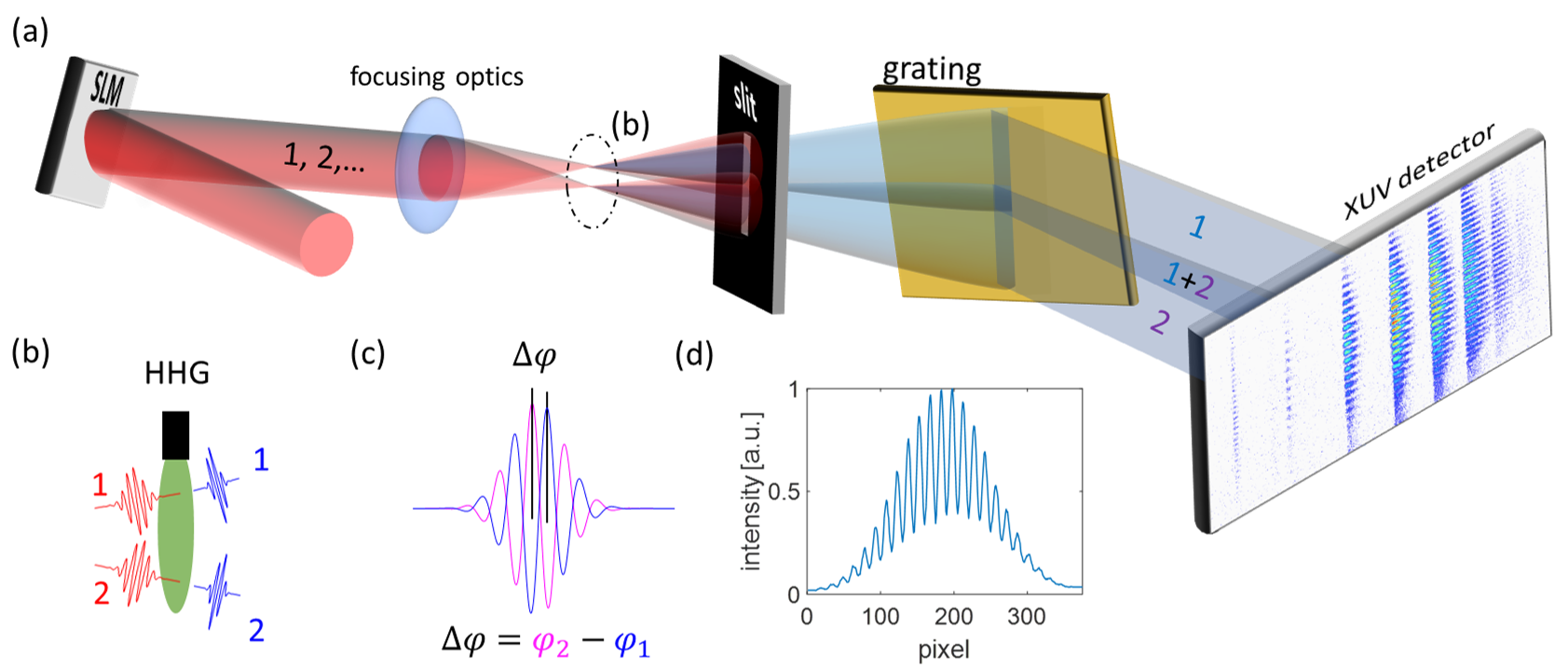
Figure 1: (a) Sketch of the experimental setup. A spatial light modulator (SLM) is used to separate the incoming beam into multiple (here two) phase locked beams. They are used to generate spatially separated but phase locked harmonics which interfere in the far field and are detected with an XUV spectrometer. (b) Schematic of the HHG in the gas jet (c) Relative phase difference and relative time delay between the interferometric beams. (d) A sample line-out of the fringes seen in the spectrometer.

As an initial experiment the stability of the interferometer is thoroughly characterized. This series of experiments can be split into two measurable quantities: resolution as how precisely the phase delay can be controlled and precision as the resolving power in phase delay. The values used for comparison are the RMS deviation from a linear phase for the resolution and the standard error for the accuracy. To demonstrate control, one fundamental beam is delayed with respect to the other by using the SLM to add an optical phase $\Delta\phi_{SLM}$, which can be tracked in the interference fringes for harmonic 2q+1, following $\Delta\phi_{2q+1}=(2q+1)\times\Delta\phi_{SLM}$.

For a light pulse traveling in vacuum, an optical phase $\Delta\phi_{2q+1}$ is equivalent to a time delay, $\Delta\tau_{(2q+1)}=\frac{\Delta\phi_{2q+1}}{2\pi}\times\frac{T_{f}}{2q+1}$ with $T_{f}$ the fundamental’s period. Fig. 2(a) shows a delay phase scan over $\pi$ rads of the 17th harmonic ($\Delta\phi_{SLM}=\pi/17$ rads of the fundamental) in 100 steps leading to a precision in the step size of 75 zs across several harmonics. The resolution is determined from the root mean square (RMS) deviation from the intended linear slope. The inset of Fig. 2(a) shows a scan with steps close to its resolution. Here, the 7th harmonic pulses are delayed in 0.2 mrad steps over 2 mrads of the fundamental (840 zs) achieving a resolution of $\,52\,$ zs. In other words, we can control two pulses that are spatially separated by 0.3 mm at 72 nm center wavelength (17.3 eV) with a precision that is only found in optical cavities. This relative stability value, equivalent to a non-local relative phase stability in the fundamental of 0.12 mrad is reached after 21 M laser shots or 350 minutes at 1 kHz rate.

Most attosecond experiments have a strong caveat, the strong fundamental co-propagates with the XUV pulses. To overcome this limitation we use Bessel-Gauss beams [26, 27]. The phase stability with these beams, reported as the standard error (100 laser shots make a measurement) as a function on number of laser shots, is shown in Fig. 2(b) for harmonics 7-11 generated in ethylene. These harmonics, used for experiments later in this paper, showed a much greater variance in brightness than the Gaussian beams. The brightest harmonic, the 11th, has the best signal to noise ratio of any harmonic and reaches a standard error of 3 zs (0.079 mrad) after 4 M shots (65 minutes at 1 kHz). In contrast, the standard errors of the 15th-21st harmonics for the Gaussian experiment show a similar $1/\sqrt{N}$ shots trend but with multiple harmonics reaching sub 100 zs stabilities after 2M shots, shown in the supplemental materials section 1.

Overall, this constitutes an improvement of two order of magnitude in step size compared to earlier experiments [21] and one order of magnitude compared to other state of the art XUV-XUV delay lines [19, 15, 20].

One has to mention that with a higher repetition rate source, e.g. 50 kHz which is not uncommon for XUV sources [28] or our own upcoming source at 200 kHz [29], millions of shots could be reached within seconds making this setup a prefect candidate for high precision measurements with resolutions less than 10 zs.Ytterbium based sources can even reach repetition rates over 10 MHz [30] and will decrease the measurement time even further. A high repetition rate system could be simply integrated into a setup without needing to replace other equipment as the limiting factor for this system is the damage threshold of the SLM. This damage threshold is mostly dictated by the peak intensity of the fundamental pulses, not the average power. Liquid crystal on silicon (LCOS) SLMs have been tested with average powers nearly two orders of magnitude higher than those used here [31, 32, 33].

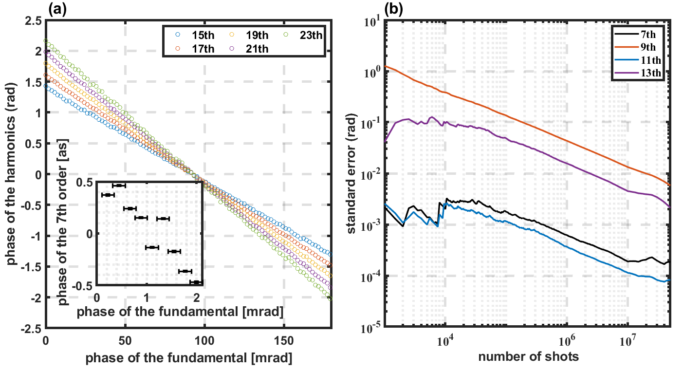
Figure 2: (a) The phase evolution of harmonics 15-21, generated in Ar, as a function of fundamental phase difference. These harmonics show resolutions of around 75zs. Inset, a finer scan of the phase evolution in time of the 7th harmonic (113 nm) showing a resolution of 52 zs (0.86 mrad). Here the resolution is close to the intended step size of the scan (84 zs) and is shown as the horizontal error bars. The vertical error bars show the precision achieved (10 zs) (b) Standard error when characterizing the phase of one mask as a function of laser shots. This is shown for harmonics 7-11 generated from a bessel-like beam.

While we demonstrated the precision required to make interferometric measurements on the Compton timescale, the question of whether they are entangled naturally arises as the interfering photons come from the same source. Beams with orbital angular momentum (OAM) have been shown to generate a high degree of entanglement [34, 35] and they have been used in HHG in the past [36, 37]. For this study, we created beams with superposed OAM beams of order $\pm 1$ so that they generate harmonics from two foci [37] which can be used for ITAS. A description of the modifications needed to accomplish these different kinds of beams can be found in the supplemental material section.

In order to check for entanglement, the XUV flux is decreased by lowering the gas pressure. Due to the coherent nature of HHG, XUV flux is dependent on the number of emitters squared [38, 39] making this a simple way to reach the photon counting limit. Photon correlations should result from any entanglement between the beams. Three beam modes are examined in this regime: a single Gaussian, two Gaussians, and superimposed OAM $\pm 1$. Initially spectral correlations are inspected. Only two-photon events are studied and a condition is imposed on the measurement: at least one photon’s wavefunction is required to have collapsed in a spectral region or "gate". Spectra with only these photons and their secondary photons are shown in Figure 3 (b) and (c). The parts of the spectra in the gates are amplified but outside of those effects they are independent of where the gate was placed. This is a commonly used method to check for correlations between two events as correlated events should deviate strongly from the ungated spectrum. In these experiments there is no spectral correlation between the two photons and they appear to be completely independent.

Additionally, figure 3(a) shows the harmonic spectra for each mode recreated with one, two, three, or four photons per laser shot. It is evident that the spectra do not depend on the number of photons detected indicating that spectral content is independent of the number of photons generated. To our knowledge, this is the first demonstration of the theoretical proposal on this regard [24]. Our experiment indicates that each photon generated through HHG indeed contains information about the entire XUV spectrum. This is a necessary condition for producing entangled photons, however, it provides no information on the entanglement between the two non-local beams.

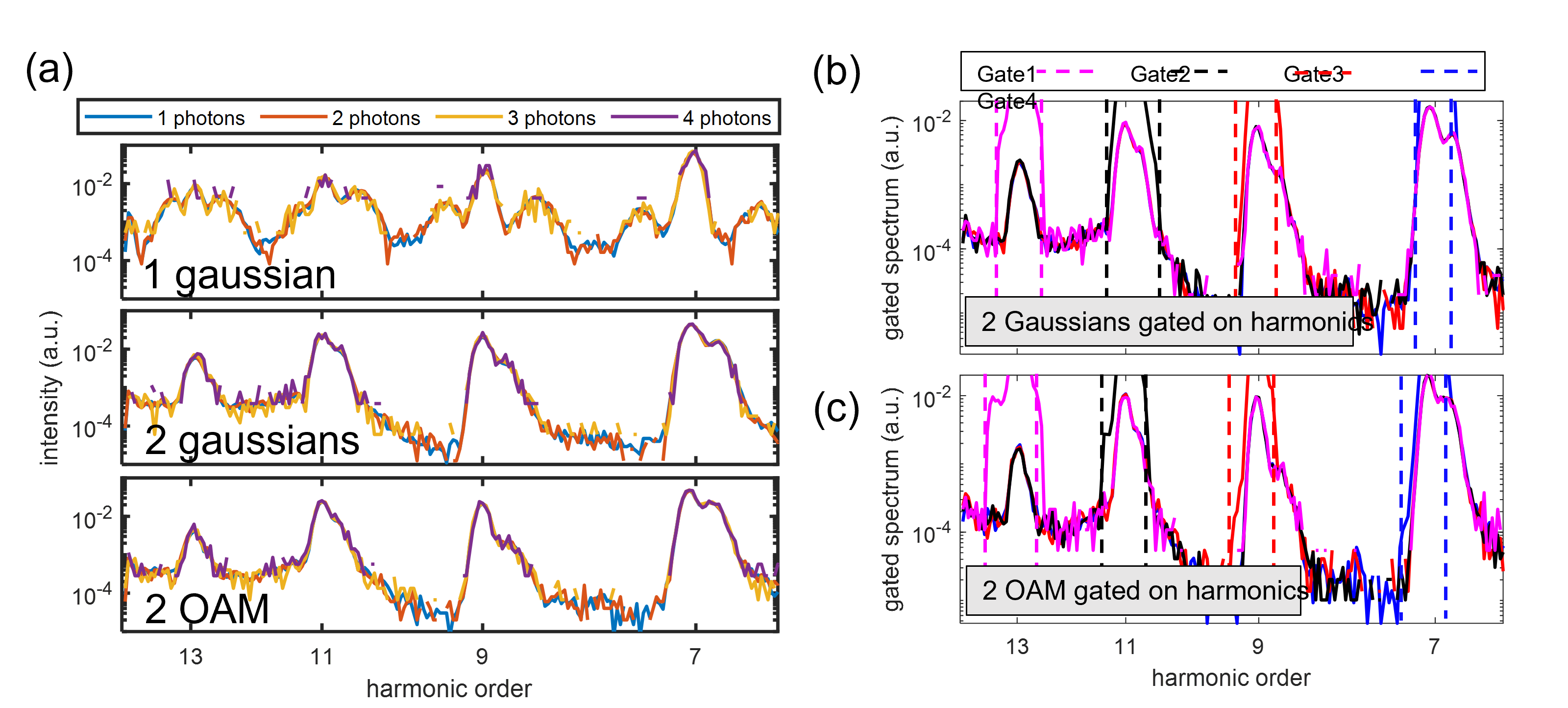
Figure 3: (a) Measured XUV spectra 1,2,3 or 4 events at a time for 3 scenarios: one gaussian beam, two gaussian beams and two beams consisting of +1 and -1 OAM. (b) (c) retrieved spectra when at least one photon is detected within the spectral gate. The gated harmonic is strongly amplified, yet the rest of the spectrum is identical. (b) and (c) depict data for two gaussian beams and two OAM beams, respectively.

We also need to rule out any spatial entanglement between the two beams in order to use pairs of XUV photons for TAS measurements, For this purpose only images which meet two conditions are examined: First, only two photons are detected. Secondly we gate the photons spatially on one of the interference fringes. The gated accumulated spectra after 16 hours is depicted in Figure 4 on the left. Here photon gates are highlighted as overlaid squares. Projections of the fringe pattern for the 7th harmonic (113nm) are shown in the right panel of Fig. 4 for three cases. Fringes reconstructed one photon at a time (orange) or two photons at a time with two different gates. The fringes within the gates are amplified again, as the gating requires at least one photon in that fringe. If the two detected photons were entangled, when collapsing the wavefunction of one, the interference pattern on the detector would get lost, as we should not be able to determine the relative phase of both photons. Fig. 4 clearly shows that the interference fringes do not change when two-photon measurements are done and we collapse the wavefunction of one photon at a time. This is the case for all the harmonics and all wavefronts we have analyzed including beams utilizing OAM as explained above.

From a homodyne perspective, the overall results show it is now possible to perform precise quantum optics measurements in the XUV with phase precisions that are normally only attainable inside optical cavities.

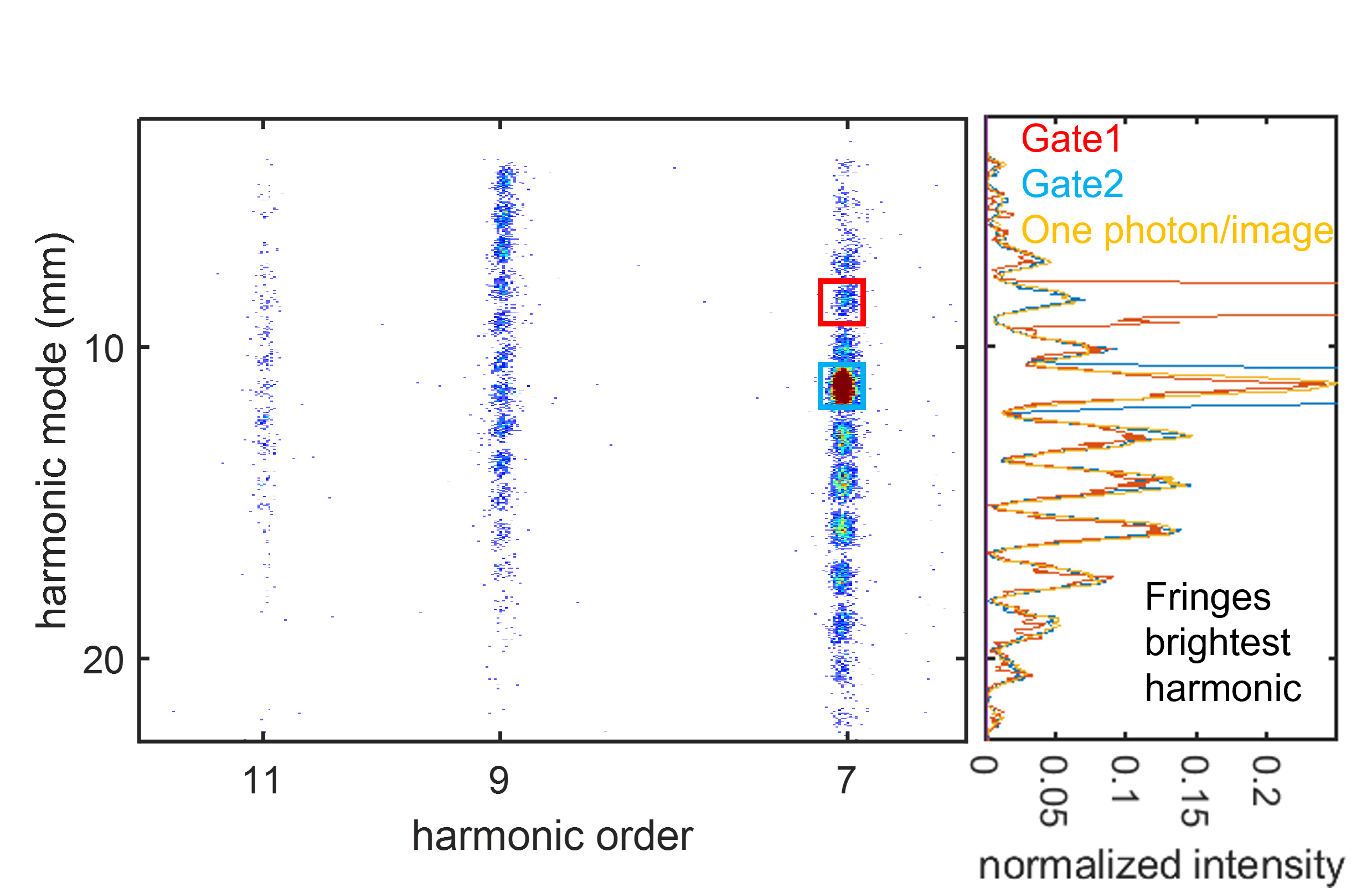
Figure 4: Accumulated image imposing two conditions on the detected photons: First, exactly two photons are detected within one image. Second, one photon is detected within a predefined gate. The gate for this image is depicted in blue. Right side shows the projection of the brightest harmonic onto the y-axis for two different gates and for the single-photon data. The gates used for these fringes are indicated in the image in red and blue.

In order to motivate the application of our approach we theoretically describe the process of the interaction of two non-local XUV beams with a medium. Details of the theoretical model are found in the supplemental section 5. Briefly, as photons travel through a medium there are secondary light emissions due to the induced dipole acceleration, with the dipole given by $\mathbf{d}(t)\!=\!\langle\Psi(t)\lvert\mathbf{\hat{d}}\rvert\Psi(t)\rangle$[40]. In our case there will be two spatially-separated sources of emission as depicted in Fig. 1 which we assume to be two XUV plane waves that propagate with no IR fields, as is the case with Bessel-like beam generation discussed above. The two beams will interact with two media having index of refraction $n_{\alpha}$ and optical thickness $L^{\alpha}_{S}$ where $\alpha=1,2$ represents source 1 or 2. Since the XUV flux is low, the cross section for non-linear processes is negligible and only the linear response is calculated. For light linearly polarized in the z direction, and following the symmetry of the two sources with respect to the spectrometer, only the $z-$ component of the field remains, see discussion in Sec. 5 and Fig. S4 in supplemental material.

Experimental spectra are determined by the time-average of the Fourier transform of the Poynting vector at point $\boldsymbol{r}_{d}$ on the detector plane and frequency $\omega$:

$$\langle\mathbf{S}_{D}\rangle(\mathbf{r}_{d},\omega)=\Big{\lvert}\sum_{\alpha}E^{(\alpha)}_{z}(\mathbf{r}_{d},\omega)\Big{\rvert}^{2}\,\text{{e}}_{r},$$ (1)

Which gives a simple equation for the detected spectrum as a sum of each beam’s spectral intensity along with an interference term, $\langle\mathbf{S}_{D}\rangle(\mathbf{r}_{d},\omega)\!\!=\!\!I^{(1)}(\mathbf{r}_{d},\omega)+I^{(2)}(\mathbf{r}_{d},\omega)+I_{\text{int}}(\mathbf{r}_{d},\omega)$, where $I_{\text{int}}(\mathbf{r}_{d},\omega)$ is given by,

$$I_{\text{int}}(\mathbf{r}_{d},\omega)\propto\big{\lvert}d^{(1)}_{z}(\omega)\big{\rvert}\,\big{\lvert}d^{(2)}_{z}(\omega)\big{\rvert}\,\cos\big{[}\phi^{(1)}_{dip}(\omega)-\phi^{(2)}_{dip}(\omega)+\Delta\theta_{\text{opt}}(\mathbf{r}_{d},\omega)\big{]},$$ (2)

with

$$\phi^{(\alpha)}_{dip}(\omega)\equiv\arg\big{[}\tilde{\ddot{d}}^{(\alpha)}_{z}(\omega)\big{]},$$ (3)

the spectral phase of the dipole acceleration in sample $\alpha$ and $\Delta\theta_{\text{opt}}$ is the difference in optical paths between the two beams. The argument in the $\cos$ term in Eq. (2) is a function of the relative phase between the dipole distributions within each sample which contains the fingerprints of the quantum dynamics triggered by the incident fields. This difference represents the experimentally measured change in phase when some parameter e.g., relative CEP phase, time delay, etc, of the field interacting with one of the sources is varied.

In our numerical simulations detailed in the supplemental section 7, we use Argon as a prototype. The multi-electron dynamics in Argon are treated in the context of the Time-Dependent Configuration Singles (TDCIS) which approximates correlated multi-electron dynamics as a linear combination of channel-resolved correlated electron-hole excitations from the neutral Hartree-Fock ground state to initially unoccupied Slater determinants describing single electron-hole excitations [41].

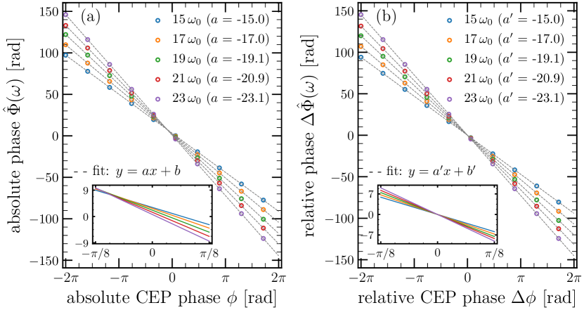
Figure 5: Numerical Simulations of the dipole acceleration induced by an XUV pulse in Ar. (a) Absolute spectral phase of the dipole acceleration $\phi^{(\alpha)}_{dip}(\omega)$ as defined in Eq. 3 for different harmonic frequencies, $\omega=(2k\!+\!1)\omega_{0}$, as a function of the absolute CEP of the IR field generating harmonics in arm 1. (b) Spectral phase of the interfering term of the Poynting vector Eq. 2 as a function of the relative CEP phase of the IR field generating harmonics.

3 Discussion

Electronic and molecular dynamics

In the case where the optical phase is constant, only dipole contributions are present and it is clear that measurements will yield information about the dipole phase. To demonstrate this point, in Fig. 5(a) we show the calculated absolute dipole acceleration phase, induced by an XUV pulse in Ar (in arm 1), as a function of the CEP of the IR generating pulse. In comparison, panel(b) shows the full argument of the cosine of the interference term in Eq. 2 under the same conditions. From the figures we can clearly see the dipole phase evolution of the target plotted in panel (a) is equivalent to the argument of Eq. 2 shown in panel (b) up to a constant $\Delta\theta_{\text{opt}}(\mathbf{r}_{d},\omega)$. A comparison with an equivalent experimental measurement shown in Fig. 2 shows an incredible agreement between theory and experiment.

Of special interest are cases where the induced dipole is controlled by a third beam that could be weak (perturbative) or intense(non-perturbative). This opens the door for interferometric transient absorption spectroscopy methods, where the observable is not restricted to only the absolute value of dipole but can also measure phase. Thus, we could have access to the phase of a quantum wavepacket either bound or in the continuum. An example is the dynamical study of molecular ro-vibrational and/or electronic wavepackets. In both cases one or more pulses populate a superposition of excited states creating wavepackets with an overall phase.

Finally, with the resolution 3 zs, we could perform experiments to test temporal aspects of QED. For example, tests of the radiation reaction time at the Compton characteristic timescale.

Interferometric 3D imaging with sub-nm resolution

Another possible application of our separated beam interferometer is for 3D imaging of small samples by measuring changes in the fringe patterns due to differences in optical path as a sample is moved through the beam. To show how our interferometric technique could be used, we start with Eq. 2 and in particular, the term $\Delta\theta_{\text{opt}}(\mathbf{r}_{d},\omega)$. Contributions to the geometrical phase come from the difference in optical paths from either source. So far, we have assumed that XUV pulses travel through the same medium and that the interacting medium has an identical composition. This assumption doesn’t need to be so however. If instead source 1 travels through a medium with index of refraction $n_{1}$ and thickness $L^{1}_{S}$ while source 2 travels through $n_{2}$, $L^{2}_{S}$, then our interferometer will measure a phase difference, $\Delta\theta_{\text{opt}}(\mathbf{r}_{d},\omega)=-\omega/c\times(n_{1}L^{1}_{S}-n_{2}L^{2}_{S})$. For 3D imaging of a sample that scans across XUV beam 2, under vacuum, the phase difference reduces to, $\Delta\theta_{\text{opt}}(\mathbf{r}_{d},\omega)=(\omega/c)n_{2}L(x,y)$, where $L(x,y)$ is the thickness profile of the sample being imaged. With a phase precision of 0.08 mrad in the 11th harmonic (72 nm), we could be able to measure thickness profiles with a resolution of $1\times 10^{-3}$ nm = 1 pm. While images taken in this fashion only provide access to a convolution of the optical mode profile and the sample, having access to relative depth profiles with this resolution could be revolutionary.

Non-local measurements in condensed matter

Another possibility of using two quantum equivalent XUV photons is the exploration of true non-local measurements in solids through photoelectron spectroscopy, or the so-called time-resolved angle photoelectron spectroscopy (trARPES) [42, 43, 44]. Theoretical proposals to use two-electron ARPES measurements to uncover correlations have been discussed in the past [45, 46]. However, the proposed measurements only involved local electron pairs. Our non-local equivalent XUV photons could probe correlations in a solid across macroscopic distances while still preserving the energy and momentum resolution power of ARPES. This, we argue, could open the door to new set of experiments to explore and resolve the spatial and temporal extent of quasi-particle correlations.

Concluding remarks

In this work we present a simple methodology for the generation and control of two quantum equivalent XUV photons with high precision using an SLM. The pair of photons are part of two attosecond pulse trains that co-propagate but are spatially separated. By using Bessel-like beams for the fundamental, we guarantee XUV propagation without the presence of the generating strong fields. In the far field the two XUV beams interfere and measurements of this interference allows for a precise determination of the relative phase and temporal jitter. The delay between the two photons can be controlled with a resolution of 52 zs and measured with a precision of 3 zs in the 11th harmonic.

We have also performed photon counting experiments, recreating full HHG spectra with one, two, three and four photons. These measurements allowed us to establish that each photon carries with it, information of the entire HHG spectrum. Additionally, after collapsing the wave function of one photon at a time, in the two-photon experiment, we showed that interference is still present leading us to conclude that photons emerging from each foci are not entangled.

We have also presented a theoretical framework on the relationship of the observed interference pattern and the phase of the quantum state of a target, through the dipole phase difference. The framework allows for a straightforward way of generalizing attosecond transient absorption spectroscopy to interferometric measurements providing values for the dipole phase.

Finally, we discussed applications of the methodology to several possible measurements.

4 Methods

Experimental Setup

The experimental setup is depicted in in the main paper in Fig. 1(a). A titanium sapphire laser (2.5 mJ, 30 fs, 1 kHz) is incident on an SLM, which divides the light into two phase locked pulses. These pulses are imprinted with two interwoven linear wavefronts, which focus into two separate locations. Depending on the focusing optics used these foci can be Gaussian, Bessel-like or generated via the interference of $\pm 1$ OAM beams. The details of how to achieve the different foci used in these experiments can be found in the supplemental materials, sections 1, 2, and 3. In all cases the foci are used to generate XUV light via HHG in a thin gas target, see Fig. 1(b). It has been shown that the SLM only adds a small amount of temporal chirp and that both beams are shorter than 40 fs[22]. The generated harmonics preserve the phase locked nature of the fundamental beams and are used as a precise, self-referencing interferometer, as has been demonstrated in previous work [21]. Later, the interference of the two HHG beams is detected in an XUV spectrometer and used to measure the phase difference between the beams. The SLM used for all experiments is a Meadowlark XY Phase series 512L. It is a LCOS device with a resolution of 512x512 pixels covering 8x8 mm and a bit of depth of 14. The high bit depth allows fine control over the phase from $0$ to $2\pi$ in $2^{14}$ steps, resulting in a minimum delay step size of 160 zs for 800 nm light. This limit can be lowered further by using masks with irrational slopes as shown by Harrison et al[22]. The aluminum back mirror of the SLM has a total reflection efficiency of around 50% at 800 nm leaving 1.25 mJ to be split between the two beams. By switching to an SLM with dielectric back mirror up to double the power would be available in the HHG process thus a higher cut-off and flux are easily reachable. The HHG gas jet is a fused silica capillary nozzle mounted on an in-vacuum 3-D stage. An 4D Aligna TEM beam-pointing system is used before the SLM to compensate for long term drift in the beam line, allowing for extended measurement periods.

Detectors

For this work two different XUV spectrometers were employed.

For harmonics >20 eV a grazing incidence spectrometer based on a McPherson design is used with a curved 600 g/mm XUV grating. The grating is designed for 1 nm - 65 nm, i.e. 19 eV - 1240 eV. The CCD recording the images is a low noise Andor Newton DO940P-BEN with 2048 x 512 pixel and a pixel size of $13.5~{}\mu m$. Due to the design of the spectrometer a 300 nm thick aluminum foil is needed to filter the fundamental 800 nm beam as the scattered light would overexpose the camera.

For the photon counting and lower harmonics a Shimadzu (30-007) unequally spaced curved-groove laminar type replica grating was used, which is designed for 50 nm - 200 nm, i.e. 6 eV - 25 eV. A micro channel plate (MCP) stack and phosphor screen is placed in the focus of the grating and gets imaged by a low noise camera (Hammamatsu Orca Flash 4.0, C11440). The advantage of this spectrometer design is that the fundamental light does not produce any scattering and that the zero order can be easily blocked, consequently no metal filter is needed. Additionally, the fast low noise camera allows for single shot measurements due to a short exposure time ($<1~{}ms$) as well as the capability to be triggered to the lasers repetition rate.

Theory

Full detail of the theoretical work can be found in the Supplemental material.

Acknowledgements

We thank fruitful discussions with Peter Brunt of AVR Optics. Research supported by US Department of Energy, Office of Science, Chemical Sciences, Geosciences, & Biosciences Division grant DE-SC0019098 and DE-SC0023192.

Ethics declarations

The authors declare no competing interests.

Generation and control of non-local quantum equivalent extreme ultraviolet photons: supplemental document

1 Phase Mask Creation for Gaussian Beams

The multiple beam phase masks for the SLM are generated by intertwining two opposing linear slopes. This is done by randomly assigning each pixel to a particular mask. The randomization prevents structures from forming increasing the diffraction efficiency of the device. It also allows us to arbitrarily distribute the light between the beams by biasing the random number assignment, for example giving one beam 50$~{}\%$ of the pixels and the other 40$~{}\%$ would give a 20$~{}\%$ difference between the intensities at the focus, which corresponds to an unbalanced scheme. In such a case, the extra ten percent is put in a third beam that focuses far away from the others and doesn’t affect the experiment. The stability of a balanced scan (15th - 21st harmonic) as well as a sample line cut of one harmonic (7th) for the unbalanced case is given in figure S1(a) and (b), respectively. Even within only $3\times 10^{6}$ shots these harmonics reach a precision of under 100-zs. The unbalanced data was taken with the MCP-Phosphor detector scheme and thus the spatial resolution is slightly limited, yet the fringes are clearly resolved.

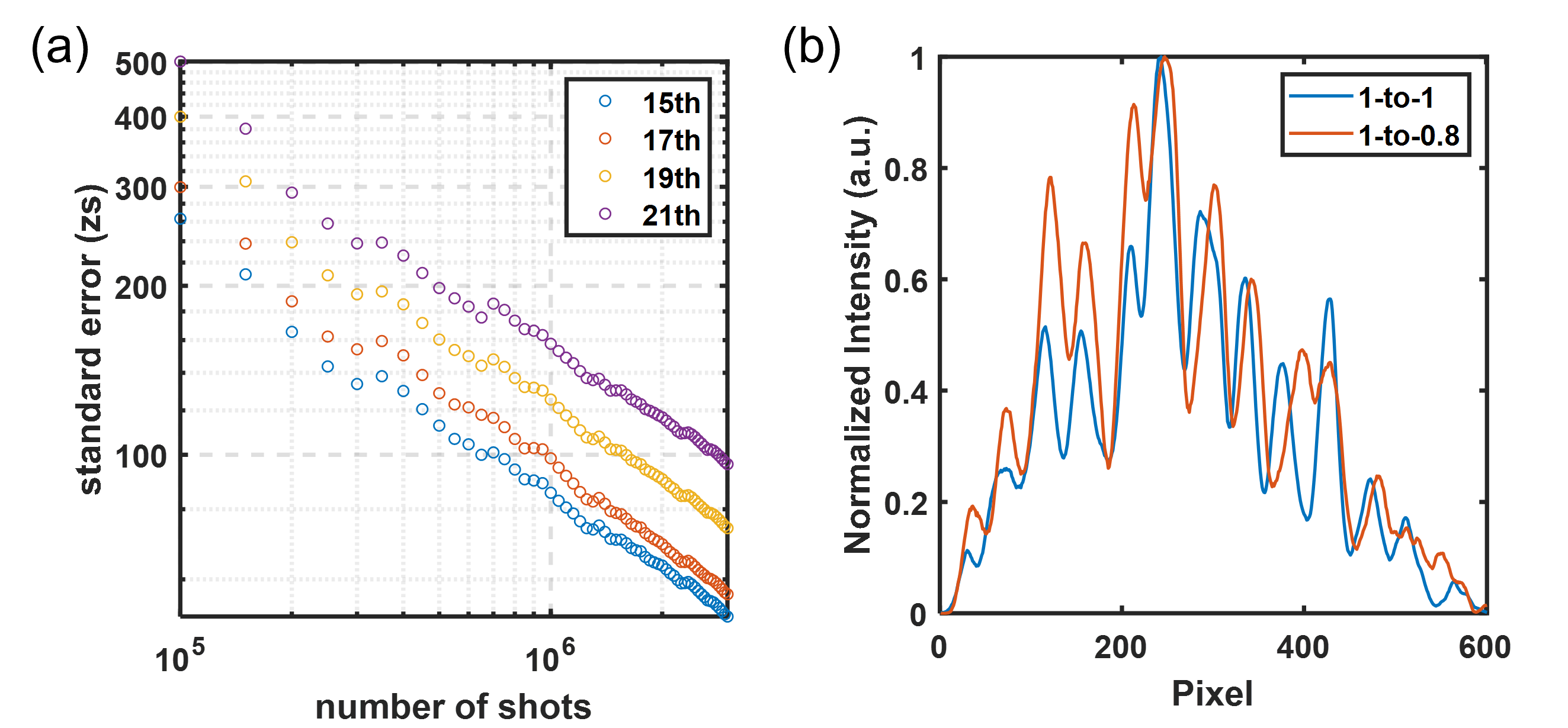
Figure S1: (a) Standard error in zs of two balanced Gaussian beams as a function of the number of shots. Data is shown for the 15th - 21st harmonic. (b) Unbalanced fringes for the 7th with the fundamental beam split 1-to-1 and 1-to-0.8

Additionally, this method is not limited to two beams but can be scaled depending on the pixel resolution of the SLM and the beam size impinging on it.

2 Orbital Angular Momentum beam generation

To check for entanglement beams with superimposed $\pm 1$ units of orbital angular momentum (OAM) are created in the following scheme, as presented before by Tross et al. [37]. In the same manner as for the Gaussian beams pixels were chosen at random and one of two different phase masks is applied. The first phase mask continuously ramps up the phase circularly from 0 to 2$\pi$, whereas the other starts at 2$\pi$ and decreased circularly to 0. It is important that the phase jump between 0 and 2$\pi$ happens at the same spot on the SLM. The resulting co-linear beam is a superposition of $\pm 1$ OAM and focused via a lens develops two distinct foci, which can be used for HHG.

3 Bessel-like beam generation

To switch from Gaussian beams to Bessel-like beams only one optical element needs to be added to the optical system: an axicon after the lens. Such beams have been used in the past for HHG in a thin gas jet [27]. Figure S2 (a) shows a typical focus achieved when using these beams in conjunction with two different wavefronts as in the Gaussian case. Figure S2 (b) shows the far field with zero intensity on axis, Well suited for IR-free experiments.

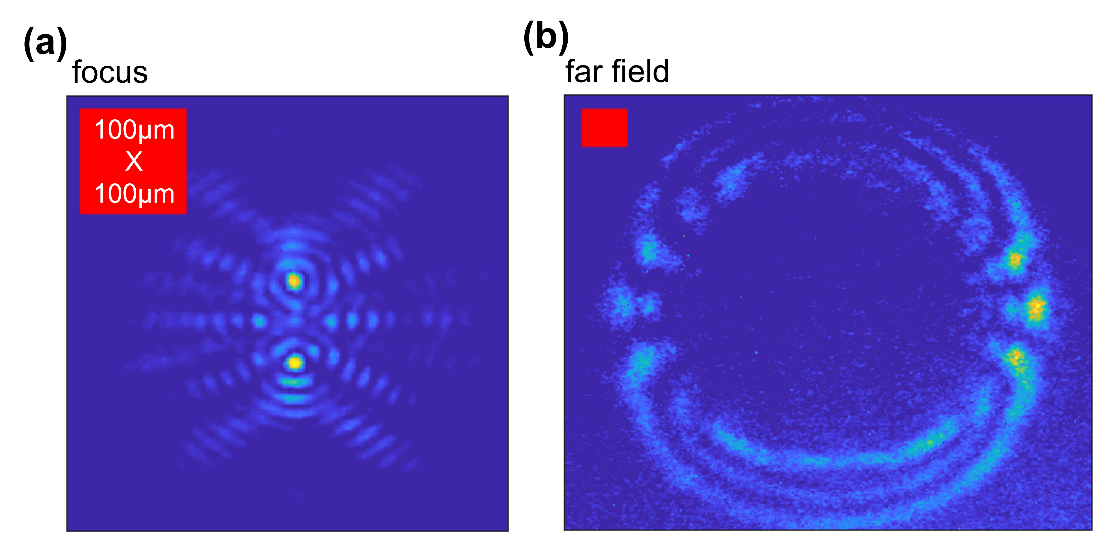
Figure S2: (a) The focus of two Bessel-like beams with two different interwoven wavefronts. (b) Far field of the beams depicted in (a).

4 Phase evaluation of the experimental data

To extract reliable phase information from the collected images several steps are taken. First, each harmonic gets projected on the spatial axis such that the fringes are obtained for each (a sample for one harmonic is given in figure S3). Second, the projected harmonic is background subtracted and zero padded with $2^{10}$ zeros on each side. Third, a Hamming filter is applied to suppress windowing effects. As a forth step the fast Fourier-transform (FFT) of the data is calculated, see figure S3 (c) for the magnitude of the FFT. The fringes are clearly visible as a distinct frequency. The phase of this frequency gives the phase difference between the two beams with some constant offset.

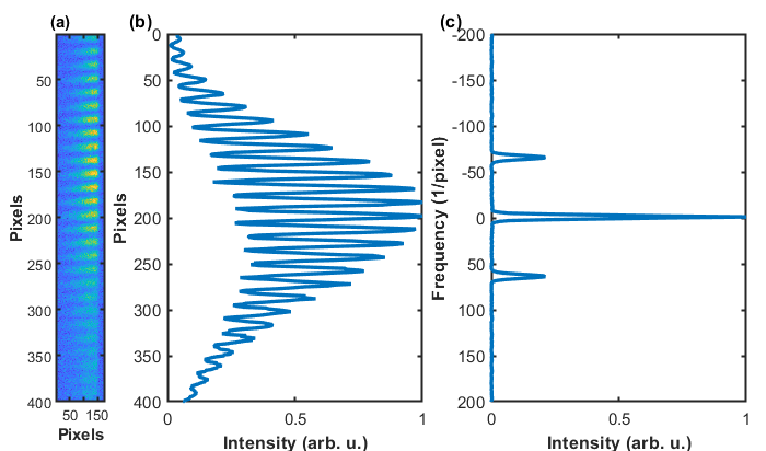
Figure S3: (a) A zoomed in harmonic showing fringes. (b) An integrated lineout of the fringe in (a) with a hamming filter applied. For the analysis this line is also zero-padded but the padding is cropped out for clarity. (c) The Fourier Transform of the lineout shown in (b). This figure is again cropped for clarity. The only peaks present are those corresponding to the DC component and the frequency of the fringes.

5 Theoretical model

5.1 Microscopic Description of Laser-Induced Electromagnetic Radiation

To describe propagation of the incident IR/XUV fields through the samples $\alpha=1,2$ (see main text), we solve the Maxwell equations in the Lorenz gauge. We first consider the generation of electromagnetic radiation due to the interaction of the incident, external radiation with a single atom. Macroscopic effects will be included as a second step, as described in Sec. 5.2. The homogeneous solution to the Maxwell equations (vanishing charge density and current density ) describe the propagation of the incident field in the absence of the samples, i.e., free space, whereas the particular solution to the inhomogeneous equation describe the radiative emission response due to the non-stationary charge distributions and charge currents triggered by the (total) field in the medium. Propagation of the incident field through the medium thus results in the emission of an effective secondary radiation source that adds up to the incident field to obtain the effective, propagated field. To obtain the particular solution, we first solve the Maxwell equations for the scalar and vector potentials, which satisfy,

$$\boldsymbol{\square}\,\Phi(\boldsymbol{r},t) = \rho(\boldsymbol{r},t)/\epsilon_{0}\,,$$ (S1a)

$$\boldsymbol{\square}\,\boldsymbol{A}(\boldsymbol{r},t) = \mu_{0}\boldsymbol{j}(\boldsymbol{r},t)\,,$$ (S1b)

with $\boldsymbol{\square}\equiv\boldsymbol{\nabla}^{2}\,-\,\partial^{2}/\partial t^{2}$ and where $\rho(\boldsymbol{r},t)$ and $\boldsymbol{j}(\boldsymbol{r},t)$ denote the charge density and current density distributions in the medium generating the secondary radiation field. Both, $\rho(\boldsymbol{r},t)$ and $\boldsymbol{j}(\boldsymbol{r},t)$ are treated quantum mechanically. At the single-atom level, the time-dependent dipole moment is given by $\boldsymbol{d}(t)=\int\boldsymbol{r}\rho(\boldsymbol{r},t)\,d^{3}\boldsymbol{r}$, with $\rho(\boldsymbol{r},t)\!=\!\langle\Psi(t)|\boldsymbol{r}\rangle\langle\boldsymbol{r}|\Psi(t)\rangle$ the charge probability density distribution and $|\Psi(t)\rangle$ the state vector obeying the time-dependent Schrödinger equation,

$$i(\partial/\partial t)\,|\Psi(t)\rangle=\hat{H}(t)|\Psi(t)\rangle\,,$$ (S2)

with $\hat{H}(t)\!=\!\hat{H}_{0}+\hat{V}(t)$ with $\hat{H}_{0}$ and $\hat{V}(t)$ denoting the field-free and interaction Hamiltonians respectively. Solutions of (S1) obeying causality are given by the “retarded" scalar and vector potentials,

$$\Phi(\boldsymbol{r},t) = \dfrac{1}{4\pi\epsilon_{0}}\,\int\dfrac{\rho(\boldsymbol{r}^{\prime},t_{r})}{|\boldsymbol{r}-\boldsymbol{r}^{\prime}|}\,\,d^{3}\boldsymbol{r}^{\prime}\,,$$ (S3a)

$$\boldsymbol{A}(\boldsymbol{r},t) = \dfrac{\mu_{0}}{4\pi}\,\int\dfrac{\boldsymbol{j}(\boldsymbol{r}^{\prime},t_{r})}{|\boldsymbol{r}-\boldsymbol{r}^{\prime}|}d^{3}\boldsymbol{r}^{\prime}\,,$$ (S3b)

with $t_{r}\equiv|\boldsymbol{r}-\boldsymbol{r}^{\prime}|/c$ the retarded time and $c$ is the velocity of light in vacuum. In the far-field region, and to the lowest order approximation in $r/r^{\prime}$, (S3) takes the asymptotic form,

$$\boldsymbol{A}(\boldsymbol{r},t) \underset{r\gg r^{\prime}}{=} \dfrac{\mu_{0}}{4\pi r}\,\boldsymbol{\dot{d}}(t-r/c)\,.$$ (S4a)

$$\Phi(\boldsymbol{r},t) = \dfrac{Q_{e}}{4\pi\epsilon_{0}r}+\dfrac{\mu_{0}c}{4\pi r}\,\,\hat{\text{{e}}}_{r}\cdot\boldsymbol{\dot{d}}(t-r/c)\,,$$ (S4b)

with $Q_{e}\!=\!\int d^{3}\boldsymbol{r}^{\prime}\rho(\boldsymbol{r}^{\prime},t^{\prime})$ the total charge. In deriving (S4a) we have assumed that the current of probability density passing through a closed surface of arbitrarily large radius from the radiation source can be neglected. Weak ionization probabilities are therefore implicit in the model. In spherical coordinates, the magnetic field $\boldsymbol{B}(\boldsymbol{r},t)=\boldsymbol{\nabla}\times\boldsymbol{A}(\boldsymbol{r},t)$ becomes

$$B_{r}(\boldsymbol{r},t) = 0\,,$$ (S5a)

$$B_{\vartheta}(\boldsymbol{r},t) = \mathcal{M}_{x}(r,t^{\prime})\cos\varphi-\mathcal{M}_{y}(r,t^{\prime})\sin\varphi\,,$$ (S5b)

$$B_{\varphi}(\boldsymbol{r},t) = \mathcal{M}_{x}(r,t^{\prime})\cos\vartheta\cos\varphi-\mathcal{M}_{z}(r,t^{\prime})\sin\vartheta+\mathcal{M}_{y}(r,t^{\prime})\cos\vartheta\sin\varphi\,.$$ (S5c)

with $\mathcal{M}_{j}(r,t^{\prime})\!=\!-(\mu_{0}/4\pi)\big{[}\dot{d}_{j}(t\!-\!r/c)/{r^{2}}+\ddot{d}_{j}(t\!-\!r/c)/(rc)\big{]}$, and where $d_{j}$, for $j=(x,y,z)$, indicates the Cartesian components of the dipole moment. Finally, $\dot{d}_{j}(t^{\prime})\equiv(\partial/\partial t)\,d(t-r/c)$ and $\ddot{d}_{j}(t^{\prime})\equiv(\partial^{2}/\partial t^{2})\,d(t-r/c)$ denote the dipole velocity and acceleration, respectively. The electric field, $\boldsymbol{E}(\textbf{r},t)\!=\!-\boldsymbol{\nabla}\Phi(\boldsymbol{r},t)\!-\!(\partial/\partial t)\,\boldsymbol{A}(\boldsymbol{r},t)$ due to the charge distribution and current density reads

$$E_{r}(\boldsymbol{r},t) = Q_{x}(r,t^{\prime})\sin\vartheta\cos\varphi-Q_{y}(r,t^{\prime})\sin\vartheta\sin\varphi+Q_{z}(r,t^{\prime})\cos\vartheta\,,\quad\quad$$ (S6a)

$$E_{\vartheta}(\boldsymbol{r},t) = G_{x}(r,t^{\prime})\cos\vartheta\cos\varphi+G_{y}(r,t^{\prime})\cos\vartheta\sin\varphi-G_{z}(r,t^{\prime})\sin\vartheta\,,$$ (S6b)

$$E_{\varphi}(\boldsymbol{r},t) = G_{y}(r,t^{\prime})\cos\varphi-G_{x}(r,t^{\prime})\sin\varphi\,,\quad\quad$$ (S6c)

with $Q_{j}(r,t^{\prime})=-(\mu_{0}c/2\pi)\big{[}\dot{d}_{j}(t^{\prime})/{r^{2}}+d_{j}(t^{\prime})/(r^{3}c^{-1})\big{]}$, and $G_{j}(r,t^{\prime})=-(\mu_{0}c/4\pi)\big{[}\ddot{d}_{j}(t^{\prime})/(rc)+\dot{d}_{j}(t^{\prime})/{r^{2}}+d_{j}(t^{\prime})c/{r^{3}}\big{]}$. Note that in the far-field region, only the dipole acceleration $\ddot{\boldsymbol{d}}(t^{\prime})$ contributes in (S5) and (S6) as the dipole and velocity counterparts fall off as $1/r^{3}$ and $1/r^{2}$, respectively. In the far-field region, the particular solutions for the radiation fields then become,

$$E_{\vartheta}(\boldsymbol{r},t) = \dfrac{\mu_{0}}{4\pi r}\Big{[}\ddot{d}_{z}(t^{\prime})\sin\vartheta-\ddot{d}_{y}(t^{\prime})\cos\vartheta\sin\varphi-\ddot{d}_{x}(t^{\prime})\cos\vartheta\cos\varphi\,\Big{]}\,,$$ (S7a)

$$E_{\varphi}(\boldsymbol{r},t) = \dfrac{\mu_{0}}{4\pi r}\Big{[}\ddot{d}_{x}(t^{\prime})\sin\varphi-\ddot{d}_{y}(t^{\prime})\cos\varphi\,\Big{]}\,,$$ (S7b)

$$E_{r}(\boldsymbol{r},t) = 0\,,$$ (S7c)

for the electric radiation field at the single-atom level. Conversely, for the magnetic field,

$$B_{\vartheta}(\boldsymbol{r},t) = \dfrac{\mu_{0}}{4\pi rc}\Big{[}-\ddot{d}_{x}(t^{\prime})\sin\varphi+\ddot{d}_{y}(t^{\prime})\cos\varphi\,\Big{]}$$ (S8a)

$$B_{\varphi}(\boldsymbol{r},t) = \dfrac{\mu_{0}}{4\pi rc}\Big{[}\ddot{d}_{z}(t^{\prime})\sin\vartheta-\ddot{d}_{y}(t^{\prime})\cos\vartheta\sin\varphi-\ddot{d}_{x}(t^{\prime})\cos\vartheta\cos\varphi\,\Big{]}\,,$$ (S8b)

$$B_{r}(\boldsymbol{r},t) = 0\,.$$ (S8c)

Comparing (S7) and  (S8), $B_{\vartheta}(\textbf{r},t)=-E_{\varphi}(\boldsymbol{r},t)/c$, and $B_{\varphi}(\textbf{r},t)=+E_{\vartheta}(\boldsymbol{r},t)/c$. In the far-field limit, the corresponding Poynting vector $\boldsymbol{S}(\boldsymbol{r},t)\!=\!\boldsymbol{E}(\boldsymbol{r},t)\times\boldsymbol{B}(\boldsymbol{r},t)/\mu_{0}$ measuring the energy-flux density per unit area per unit time, reduces to

$$\boldsymbol{S}(\boldsymbol{r},t)=\sqrt{\dfrac{\epsilon_{0}}{\mu_{0}}}\,\big{[}|E_{\vartheta}(\boldsymbol{r},t)|^{2}+|E_{\varphi}(\boldsymbol{r},t)|^{2}\big{]}\,\hat{\text{{e}}}_{r}\,.$$ (S9)

5.2 Macroscopic Propagation and Volume Averaging

Making use of the property $\mathcal{F}\{d(t-r/c)\}(\omega)\!=\!e^{i\omega r/c}\mathcal{F}\{d(t)\}(\omega)$, the frequency distribution of the electric field component defined by the first term in the RHS in (S7a) at a point $\boldsymbol{r}_{d}=(x_{d},y_{d},z_{d})$ on the detector plane due to the atomic charge distribution located at the position $\boldsymbol{r}_{i}=(x_{i},y_{i},z_{i})$ is given by

$$E_{\vartheta}(\boldsymbol{r}_{d}-\boldsymbol{r}_{i},\omega)=\dfrac{\mu_{0}}{4\pi|\boldsymbol{r}_{d}-\boldsymbol{r}_{i}|}\,\sin{\vartheta_{d,i}}\,\,e^{i\omega|\boldsymbol{r}_{d}-\boldsymbol{r}_{i}|/c}\,\hat{\ddot{d}}_{z}(\omega;[E_{ext}(\boldsymbol{r}_{i})])\,.$$ (S10)

The position vectors $\boldsymbol{r}_{d}$ and $\boldsymbol{r}_{i}$ are defined with respect to the coordinate system $\mathcal{R}=(x,y,z)$ shown in Fig. S4 whilst $\theta_{d,i}$ denotes the spherical polar angle defined by an arbitrary $\tilde{z}-$ axis in the atomic frame of reference centered at $\boldsymbol{r}_{i}$ and the vector $\boldsymbol{r}_{d}-\boldsymbol{r}_{i}$. The quantity $\hat{\ddot{d}}_{z}(\omega;[E_{ext}(\boldsymbol{r}_{i})])$ in (S10) stands for the Fourier Transform of the atomic dipole acceleration obtained by solving the time-dependent Schrödinger equation for the atomic system located at $\boldsymbol{r}_{i}$ in $\mathcal{R}$ subject to the electric field $E_{ext}(t,\boldsymbol{r}_{i})$. The latter may or may not be a function of the position $\boldsymbol{r}_{i}$ within the samples $\alpha=1,2$ macroscopically characterized by the refractive index $n_{\alpha}(\omega)$ in Fig. S4. Analytical models allowing to obtain closed-form expressions for HHG radiation fields that incorporates macroscopic effects have been obtained by solving the 1D-Maxwell equations in a infinitely thin, infinitely long gas distribution [47] as well as by accounting for non-uniform intensity distribution of focused Gaussian beams in the slowly-varying envelope approximation [40]. Here, we resort to define the “net” electric field originating from the sample $\alpha$ as net contribution of the individual atomic charge distributions within each sample, namely,

$$E^{(\alpha)}_{\vartheta}(\boldsymbol{r}_{d},\omega)=\sum^{N_{\alpha}}_{i=1}E_{\vartheta}(\boldsymbol{r}_{d}-\boldsymbol{r}_{i},\omega)\,,$$ (S11)

with $N_{\alpha}$ the number of microscopic charge distributions (atoms) in the sample $\alpha$ and $E_{\vartheta}(\boldsymbol{r}_{d}-\boldsymbol{r}_{i},\omega)$ defined in (S10). We approximate (S11) according to

$$E^{(\alpha)}_{\vartheta}(\boldsymbol{r}_{d},\omega)=\int_{V_{\alpha}}d^{3}\boldsymbol{r}^{\prime}\,\,\rho_{\alpha}(\boldsymbol{r}^{\prime})\,\,E_{\vartheta}(\boldsymbol{r}_{d}-\boldsymbol{r}^{\prime},\omega)$$ (S12)

with $\rho_{\alpha}(r^{\prime})$ the macroscopic density of atoms in the sample $\alpha$. Using (S10), (S12) becomes,

$$E^{(\alpha)}_{\vartheta}(\boldsymbol{r}_{d},\omega) = \dfrac{\mu_{0}}{4\pi}\int_{V_{\alpha}}d^{3}\boldsymbol{r}^{\prime}\,\,\dfrac{e^{i\frac{\omega}{c}|\boldsymbol{r}_{d}-\boldsymbol{r}^{\prime}|}}{\boldsymbol{r}_{d}-\boldsymbol{r}^{\prime}}\sin\vartheta^{\prime}_{d}\,\,\rho_{\alpha}(\boldsymbol{r}^{\prime})\,\,\hat{\ddot{d}}_{z}(\omega;[E_{ext}(\boldsymbol{r}^{\prime})])\,.$$ (S13)

In the coordinate system $\mathcal{R}$, the volume integration is given, according to Fig. S4, by,

$$\int_{V_{\alpha}}d^{3}\boldsymbol{r}^{\prime}\equiv\int^{{y_{\alpha}+\frac{\Delta y}{2}}}_{y_{\alpha}-\frac{\Delta y}{2}}\,dy^{\prime}\int^{{x_{\alpha}+\frac{\Delta x}{2}}}_{y_{\alpha}-\frac{\Delta x}{2}}dx^{\prime}\int^{{z_{\alpha}+\frac{\Delta z}{2}}}_{y_{\alpha}-\frac{\Delta z}{2}}dz^{\prime}\,,$$ (S14)

where $\Delta{x}$, $\Delta{y}$ and $\Delta{z}$ denote the dimensions of the samples in arms $\alpha=1,2$, and $\boldsymbol{r}_{\alpha}=(x_{\alpha},y_{\alpha},z_{\alpha})$ the center-of-mass position of the samples represented by the yellow ($\alpha=1$) and red ($\alpha=2$) bullets in Fig. S4. In our numerical simulations, we have set $\boldsymbol{r}_{\alpha}=(0,0,z_{\alpha})$ with $z_{2}=-z_{1}$, see vectors $\boldsymbol{r}_{1}$ and $\boldsymbol{r}_{2}$ in Fig. S4.

Close-form expressions to (S12) can be obtained by considering an homogeneous gas density, with $N_{\alpha}$ atoms per unit volume $V_{\alpha}$ in the sample $\alpha$, i.e., $\rho_{\alpha}(\boldsymbol{r}^{\prime})=N_{\alpha}/V_{\alpha}$. As a second approximation, we consider a plane-wave distribution for the incident external IR field $E_{ext}(t,\boldsymbol{r}^{\prime})$,

$$\boldsymbol{E}_{ext}(t,\boldsymbol{r}^{\prime})=\int d\omega\,\,\hat{E}_{ext}(\omega)\,e^{-i(\omega t-k(\omega)\,y^{\prime})}\,\,\hat{e}_{z}\,,$$ (S15)

see Fig. S4 for choice of coordinates, with constant spatial distribution along the propagation direction within the width of the sample. With these approximations, we may neglect the spatial dependencies of $\rho_{a}(\boldsymbol{r})\approx N_{\alpha}/V_{\alpha}$ and that of the dipole acceleration which depends implicitly on $E_{ext}(t,\boldsymbol{r}^{\prime})$, i.e., $\hat{\ddot{d}}(\omega;[E_{ext}(\boldsymbol{r}^{\prime})])\approx\hat{\ddot{d}}(\omega)$. Finally, in the fair-field limit, the distance between a point $\boldsymbol{r}_{d}$ in the detection plane and a point $\boldsymbol{r}^{\prime}$ in the sample can be approximated according to,

$$|\boldsymbol{r}_{d}-\boldsymbol{r}^{\prime}| = (y_{d}-y^{\prime})\sqrt{1+\dfrac{(x_{d}-x^{\prime})^{2}}{(y_{d}-y^{\prime})^{2}}+\dfrac{(x_{d}-x^{\prime})^{2}}{(y_{d}-y^{\prime})^{2}}}$$ (S16)

$$\approx (y_{d}-y^{\prime})+\dfrac{1}{2}\dfrac{(x_{d}-x^{\prime})^{2}}{(y_{d}-y^{\prime})}+\dfrac{1}{2}\dfrac{(z_{d}-z^{\prime})^{2}}{(y_{d}-y^{\prime})}+\dots$$

Retaining the zeroth order approximation for the denominator $1/|\boldsymbol{r}_{d}-\boldsymbol{r}^{\prime}|$ in (S13) and first order approximation in the exponents $\exp(iw|\boldsymbol{r}-\boldsymbol{r}^{\prime}|/c)$, we obtain

$$\small E^{(\alpha)}_{\vartheta}(\boldsymbol{r}_{d},\omega)=\dfrac{\mu_{0}}{4\pi}\left(\dfrac{N_{\alpha}}{V_{\alpha}}\right)\,\,\hat{\ddot{d}}_{z}(\omega)\int^{{y_{\alpha}+\frac{\Delta y}{2}}}_{y_{\alpha}-\frac{\Delta y}{2}}\,dy^{\prime}\dfrac{e^{i\frac{\omega}{c}(y_{d}-y^{\prime})}}{y_{d}-y^{\prime}}\int^{{x_{\alpha}+\Delta x/2}}_{y_{\alpha}-\Delta x/2}dx^{\prime}e^{-i\frac{\omega}{c}\frac{x_{d}}{y_{d}}\,x^{\prime}}\int^{{z_{\alpha}+\frac{\Delta z}{2}}}_{y_{\alpha}-\Delta z/2}dz^{\prime}\,\,e^{-i\frac{\omega}{c}\frac{z_{d}}{y_{d}}\,z^{\prime}}$$ (S17)

For small divergence angles $\Omega_{Z}$ and $\Omega_{X}$ depicted by the blue, resp. red lines in Fig. S4, we approximate both quantities according to its first order expansion

$$\dfrac{x_{d}}{y_{d}} \equiv \tan(\Omega_{X})\approx\Omega_{X}$$ (S18)

$$\dfrac{z_{d}}{y_{d}} \equiv \tan(\Omega_{Z})\approx\Omega_{Z}\,.$$ (S19)

With these approximations, analytical integration of (S17) finally gives

$$E^{(\alpha)}_{\vartheta}(\boldsymbol{r}_{d},\omega) = \dfrac{\mu_{0}}{4\pi\,|y_{d}|}\,N_{\alpha}\,\,\hat{\ddot{d}}_{z}(\omega)\,\,e^{i\frac{\omega}{c}(y_{d}-y_{\alpha})}\,e^{-i\frac{\omega}{c}\,x_{\alpha}\,\Omega_{X}}\,e^{-i\frac{\omega}{c}\,z_{\alpha}\,\Omega_{Z}}$$ (S20)

$$\times \mathrm{sinc}\left(\dfrac{\omega}{c}\dfrac{\Delta y}{2}\right)\,\mathrm{sinc}\left(\frac{\omega}{c}\frac{\Delta x}{2}\Omega_{X}\right)\,\mathrm{sinc}\left(\frac{\omega}{c}\frac{\Delta z}{2}\Omega_{Z}\right)\,,$$

where $E^{(\alpha)}_{\vartheta}(\boldsymbol{r}_{d},\omega)\equiv E^{(\alpha)}_{\vartheta}(\boldsymbol{r}_{d}-\boldsymbol{r}_{a},\omega)$ is a function of the center-of-mass position $\boldsymbol{r}_{a}\equiv(x_{a},y_{a},z_{a})$ of the sample $\alpha=1,2$. After integrating (S17), the volume $V_{\alpha}$ in the denominator is compensated by the same quantity that eventually appears in the numerator. Integration over a continuum and homogeneous ensemble of atomic dipoles subject to an homogeneous external field $E_{ext}(t)$ leads to a sharply focused sinc-like spatial electric field distribution as opposed to its single-atom counterpart, i.e., compare (S20) and first term in the RHS of (S7a). Finally, it is straightforward to show that the above procedure to obtain the closed-form expression for the macroscopic field in (S20) is totally equivalent to solving the well-known inhomogeneous equation in the radiation zone for the macroscopic field [40],

$$\left(\boldsymbol{\nabla}^{2}-\dfrac{\partial^{2}}{\partial t^{2}}\right)\boldsymbol{E}(\boldsymbol{r},t)=\mu_{0}\dfrac{\partial^{2}}{\partial t^{2}}\boldsymbol{P}(t)\,,$$ (S21)

for a homogeneous ensemble of $N$ atoms per unit volume $V$, with $\boldsymbol{P}(t)=N_{\alpha}\,\langle\boldsymbol{d}^{(\alpha)}(t)\rangle_{V}$ the macroscopic polarization of the sample $\alpha$ defined by the dipole density $\langle\boldsymbol{d}^{(\alpha)}(t)\rangle_{V}=(1/V)\int d^{3}\boldsymbol{r}_{i}\,\boldsymbol{d}(t;\boldsymbol{r}_{i})$, with $\boldsymbol{d}(t;\boldsymbol{r}_{i})$ the single-atom dipole moment with center-of-mass location $\boldsymbol{r}_{i}$.

6 Two-beam interferometry

An illustrative sketch of the two-pathway interferometric setup is shown in Fig. S4 setup. As the experimental observable, we consider the time-averaged flux of the Poynting vector [48, 49, 50, 40] arriving at the detector plane, i.e.,

$$\langle\boldsymbol{S}_{D}(\boldsymbol{r}_{d},t)\rangle\equiv(1/T)\int\boldsymbol{S}_{D}(\boldsymbol{r}_{d},t)\,dt\,,$$ (S22)

where $\boldsymbol{S}_{D}(\boldsymbol{r}_{d},t)\!=\!(\epsilon_{0}/\mu_{0})\,\big{|}\sum_{\alpha}\boldsymbol{E}^{\prime(\alpha)}(\boldsymbol{r}_{d}\!-\!\boldsymbol{r}_{\alpha},t)\big{|}^{2}\,\text{{e}}_{r}$, see (S9), is the instantaneous intensity (directional energy flux) of the EM radiation at a point $\boldsymbol{r}_{d}$ in the detector plane; $\boldsymbol{r}_{\alpha}=(x_{\alpha},y_{\alpha},z_{\alpha})$ the origin of coordinates associated to the sample $\alpha\!=\!1,2$ with respect to the coordinate system $x,y,z$ in Fig. S4, and $\boldsymbol{E}^{\prime(\alpha)}(\boldsymbol{r}_{d}\!-\!\boldsymbol{r}_{\alpha},t)$ the electric vector field arriving to the detector from the sample $\alpha$ after being diffracted by a system of slits of aperture function $S(x_{s},z_{s})$ located at a fixed $y_{s}=L_{S}$ with respect to the coordinate system $(x,y,z)$ in Fig. S4. Expressing $\boldsymbol{E}^{\prime(\alpha)}_{\vartheta}(\boldsymbol{r}_{d}\!-\!\boldsymbol{r}_{\alpha},t)$ in terms of its frequency components, we obtain, after time integration in (S22), the frequency distribution, denoted $\langle\boldsymbol{S}_{D}\rangle(\boldsymbol{r}_{d},\omega)$ and defined by $\langle\boldsymbol{S}_{D}\rangle(\boldsymbol{r}_{d},\omega)\equiv d\langle\boldsymbol{S}(\boldsymbol{r}_{d},t)\rangle\,/\,d\omega$, which reads,

$$\langle\boldsymbol{S}_{D}\rangle(\boldsymbol{r}_{d},\omega)=\big{|}\sum_{\alpha}\boldsymbol{E}^{\prime(\alpha)}(\boldsymbol{r}_{d}-\boldsymbol{r}_{\alpha},\omega)\big{|}^{2}\,\text{{e}}_{r}\,,$$ (S23)

with $\hat{\boldsymbol{E}}^{\prime(\alpha)}(\boldsymbol{r},\omega)\!\equiv\mathcal{F}\big{[}\boldsymbol{E}^{\prime(\alpha)}(\boldsymbol{r},t)\big{]}(\omega)\!=\!\int^{\infty}_{\infty}e^{+i\omega t}\boldsymbol{E}^{\prime(\alpha)}(\boldsymbol{r},t)\,dt$.

We consider an slit with aperture function $S(x_{s},z_{s})=\text{rect}\big{(}x_{d}/\Delta_{x}\big{)}\times\text{rect}\big{(}{z_{d}/\Delta_{z}}\big{)}$ with the aperture widths satisfying $\Delta_{x}\!\ll\!\Delta_{z}$, where $\text{rect}(x_{d}/\Delta_{x})$ denotes a rectangular function in $x_{d}$ and correspondingly for $z_{d}$. In the reference frame associated to each oscillating charge distribution (samples $\alpha=1,2$), a point $\boldsymbol{r}_{s,\alpha}=\boldsymbol{r}_{s}-\boldsymbol{r}_{\alpha}$ on the slit aperture parallel to the $y$ (incident) direction is, with the coordinate convention of (S7), then determined by $\phi_{\alpha}\approx\pi/2$ and $\theta_{\alpha}\approx\pi/2$. Consequently, according to (S7a), $E_{\vartheta}(\boldsymbol{r}_{s,\alpha},t)\approx\mu_{0}\ddot{d}_{z}(t)/4\pi r_{s,\alpha}$. This is, only the $z$-component of the dipole acceleration contributes to the RHS of (S7a). As for (S7b), the oscillations in the $x$ direction of the dipole acceleration can be neglected as the leading contribution is given by $\ddot{d}_{z}$ for an atomic system interacting with a field linearly polarized along the $z$ direction. If this condition is not fulfilled, then both,  (S7a) and (S7b) must be used in (S23). Within this configuration and making use of $\mathcal{F}\{d(t-r/c)\}(\omega)\!=\!e^{i\omega r/c}\mathcal{F}\{d(t)\}(\omega)$, the dipole acceleration $\hat{\ddot{d}}^{(\alpha)}_{z}(\omega)$ and field $\hat{E}^{\prime(\alpha)}_{z}(\boldsymbol{r}_{d},\omega)$ spectra are related, in the Fraunhoffer approximation, according to

$$E^{\prime(\alpha)}_{z}(\boldsymbol{r}_{d},\omega)=-i\frac{\mu_{0}\omega}{4\pi r_{ds}}\,\,\tilde{\ddot{d}}^{(\alpha)}_{z}(\omega)\,\,\hat{S}(k^{\alpha}_{x},k^{\alpha}_{z})e^{i\frac{\omega}{c}L_{D}}\,\,\,e^{i\frac{\omega}{c}\frac{x^{2}_{d}+z^{2}_{d}}{2\Delta L_{D}}}\,\,\,e^{i\frac{\omega}{c}n_{\alpha}L_{S}}\,\,\,e^{i\frac{\omega}{c}\frac{x^{2}_{\alpha}+z^{2}_{\alpha}}{2L_{D}}}\,,\quad$$ (S24)

with $\boldsymbol{r}_{\alpha}\!=\!(x_{\alpha},y_{\alpha},z_{\alpha})$ the origin of coordinates of the sample $S_{\alpha}$ with respect to the coordinate system $(x,y,z)$ in Fig. S4, $n_{\alpha}\equiv n_{\alpha}(\omega)$ the corresponding index of refraction; $L_{S}$ the fixed position of the slit aperture in the $\hat{e}_{y}$ direction, $L_{D}$ the detection plane position in the $\hat{e}_{y}$ direction; $\boldsymbol{r}_{d}\!=\!(x_{d},y_{d},z_{d})\!=\!(x_{d},L_{D},z_{d})$ a point in the detector plane with fixed position at $y_{d}=L_{D}$ and finally, $\Delta L_{D}\!=\!L_{D}\!-\!L_{S}$ as indicated in Fig. S4. Finally, $\hat{S}(k^{\alpha}_{x},k^{\alpha}_{z})$ is the Fourier transform of the aperture function, given by $\hat{S}(k^{a}_{x},k^{a}_{z})\!=\!\int\int S(x_{s},z_{s})\,e^{-ik^{\alpha}_{x}(\omega)x_{s}}e^{-ik^{\alpha}_{z}(\omega)z_{s}}dx_{s}dz_{s}$, evaluated at the wave numbers $k^{\alpha}_{x}(\omega)\!=\!(\omega/c)\big{(}z_{d}/{\Delta L_{D}}\!+\!n_{\alpha}(\omega)z_{\alpha}/L_{S}\big{)}$, and $k^{\alpha}_{z}(\omega)\!=\!(\omega/c)\big{(}z_{d}/\Delta L_{D}\!+\!n_{\alpha}(\omega)x_{\alpha}/L_{S}\big{)}$.

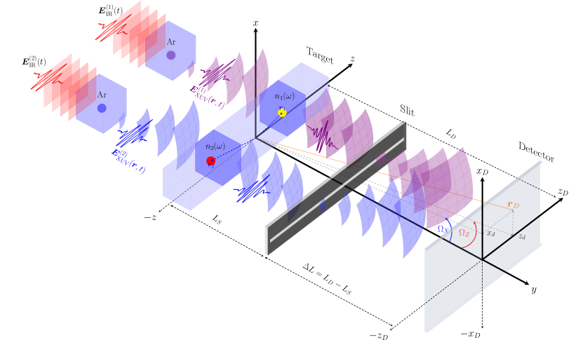
Figure S4: Idealized interferometric set up: Two XUV sources $E^{(1)}_{\mathrm{XUV}}$ and $E^{(2)}_{\mathrm{XUV}}$ generated by two phase-locked IR fields through HHG interact with two spatially separated samples, $S_{1}$ and $S_{2}$, characterized by the indices of refraction $n_{1}(\omega)$ and $n_{2}(\omega)$. After interacting with the sources, and passing trough a diffraction system (Slit) the resulting output fields interfere on the Screen/Detector plane. The output fields resulting from each arm are obtained by solving the Maxwell’s equations at the single-atom level, and are functions of the atomic dipole probed by each XUV field. Interference between both fields encodes information about the IR relative CEP phase and exhibits oscillations as a function of the spectral phase difference of each atomic dipole probed by the incident XUV fields on each sample.

With the exception of $\tilde{\ddot{d}}^{(\alpha)}_{z}(\omega)$ in (S24), all terms contain details of the diffraction and relative path differences (setup geometry and relative position of the samples). These relative phases, however, remain unchanged for fixed $\boldsymbol{r}_{d}$. Consequently, any change in spectral phase in the distribution (S23) can thus be attributed to changes in the relative spectral phase bewteen the acceleration dipoles $\tilde{\ddot{d}}^{(\alpha)}_{z}(\omega)$ in (S24) showing up in (S23), which expands according to

$$\langle\boldsymbol{S}_{D}\rangle(\boldsymbol{r}_{d},\omega) \!= \!\boldsymbol{\mathcal{I}}^{(1)}_{\text{DC}}(\boldsymbol{r}_{d},\omega)+\boldsymbol{\mathcal{I}}^{(2)}_{\text{DC}}(\boldsymbol{r}_{d},\omega)+\boldsymbol{\mathcal{I}}^{(1,2)}_{\text{int}}(\boldsymbol{r}_{d},\omega)\,,\quad$$

with the DC components,

$$\boldsymbol{\mathcal{I}}^{(\alpha)}_{\text{DC}}(\boldsymbol{r}_{d},\omega) = \boldsymbol{\mathcal{I}}_{o}(\omega)\,\,\big{|}\tilde{\ddot{d}}^{(\alpha)}_{z}(\omega)\big{|}^{2}\,\,\big{|}\hat{S}(k^{(\alpha)}_{x},k^{(\alpha)}_{z})\big{|}^{2}\,,\quad\quad$$ (S25b)

for $$\alpha=1,2 \boldsymbol{\mathcal{I}}_{o}(\omega)=(\mu_{o}/4\pi)(\omega/c)^{2}\,\textbf{\text{e}}_{r} \boldsymbol{\mathcal{I}}_{\text{int}}(\boldsymbol{r}_{d},\omega) 1 2$$. and where is an oscillating function resulting from the interference of the output fields of arms () and () after the slit,

$$\boldsymbol{\mathcal{I}}_{\text{int}}(\boldsymbol{r}_{d},\omega)=\boldsymbol{\mathcal{I}}_{o}(\omega)\!\!\prod_{\alpha=1,2}\big{|}\tilde{\ddot{d}}^{(\alpha)}_{z}(\omega)\big{|}\,\,\big{|}\hat{S}(k^{(\alpha)}_{x},k^{(\alpha)}_{z})\big{|}\,\cos\big{[}\phi^{(1)}_{dip}(\omega)-\phi^{(2)}_{dip}(\omega)+\Delta\theta_{\text{opt}}(\boldsymbol{r}_{d},\omega)\big{]}\,,$$ (S25c)

with $\phi^{(\alpha)}_{dip}(\omega)\equiv\arg\big{[}\tilde{\ddot{d}}^{(\alpha)}_{z}(\omega)\big{]}$ the spectral phase of the dipole acceleration, and $\Delta\theta_{\text{opt}}=\Delta\theta_{M}(\omega)+\Delta\theta_{P}(\omega)+\Delta\theta_{S}(\boldsymbol{r}_{d},\omega)$ an optical phase, where

$$\Delta\theta_{M}(\omega) = \omega\Delta n(\omega)L_{S}/c\,,$$ (S26a)

is a phase resulting from the refractive index difference $$\Delta n(\omega)=n_{1}(\omega)-n_{2}(\omega) S_{\alpha}$$ of the samples . Next,

$$\Delta\theta_{P}(\omega)=\dfrac{\omega/c}{2\Delta L_{D}}\left[(n_{2}(\omega)\big{(}x^{2}_{2}-z^{2}_{2}\big{)}-n_{1}(\omega)\big{(}x^{2}_{1}-z^{2}_{1}\big{)}\right]\,,$$ (S26b)

is the optical phase arising from the path difference due to the relative positions $$\boldsymbol{r}_{\alpha}$$, and finally,

$$\Delta\theta_{S}(\boldsymbol{r}_{d},\omega)=\theta^{(1)}_{S}(\boldsymbol{r}_{d},\omega)-\theta^{(2)}_{S}(\boldsymbol{r}_{d},\omega)\,,$$ (S26c)

with $\theta^{(\alpha)}_{S}(\boldsymbol{r}_{b},\omega)=\arg\big{[}\hat{S}(k^{(\alpha)}_{x},k^{(\alpha)}_{z})\big{]}$ the optical phase at the detection point $\boldsymbol{r}_{d}$ due to diffraction by the slit.

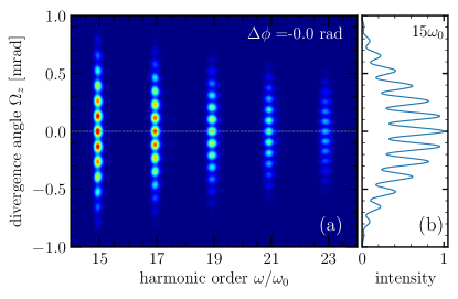
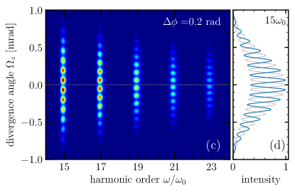
Figure S5: Numerical Simulations: (a) Frequency distribution of the volume-integrated HHG signal as a function of the divergence angle $\Omega_{z}$ defined in Fig. S4 for $\Delta\phi=0$ rad. (b) Normalized intensity profile of harmonic $15$ for $\Delta\phi=0$. (c) Same as (a) but for $\Delta\phi=0.2$ rad. (d) Intensity profiles for $\Delta\phi=0.2$ rad (solid-blue line) and $\Delta\phi=0$ rad (dashed-gray line) shown as a reference. Intensity profiles in (b) and (d) are normalized with respect to the peak intensity in (b). As a function of $\Delta\phi$, the intensity profiles of the harmonics are shifted with respect to the reference signal, i.e., compare intensity profiles shown in blue and gray colors in panel (d) . These shifts are used to extract the relative spectral phase of the atomic dipoles shown in Fig. S6(b). Geometry parameters are $x_{\alpha}=0$, $y_{\alpha}=0$ and $z_{\alpha}=\pm 50\,\mu\text{m}$ for the position of the samples $\alpha=1,2$; and $\Delta x=\Delta y=\Delta z=50\,\mu\text{m}$ for their dimensions in the $x,y,z$ direction.

7 Numerical Simulations

7.1 Quantum Dynamics and Multi-electron wave function

The spectral distribution $\hat{\ddot{d}}^{(\alpha)}_{z}(\omega)$ in (S24) is obtained from the Fourier Transform of the quantum mechanical dipole acceleration $\ddot{d}^{(\alpha)}_{z}(t)=(d^{2}/dt^{2})\,\langle\Psi^{(\alpha)}(t)|\hat{z}|\Psi^{(\alpha)}(t)\rangle$ where $|\Psi^{(\alpha)}(t)\rangle$ designates the wave function propagated under the influence of the field-free Hamiltonian $\hat{H}_{0}$ and the external IR field in arm $\alpha$ in the dipole approximation, as indicated above. We simulate the experimental HHG measurements using Argon as a prototype. The multi-electron dynamics in Argon is treated in terms of the Time-Dependent Configuration Interactions Singles (TDCIS) with active $3s$ and $3p$ orbitals. The TDCIS formalism describes single excitations of correlated electron-hole pairs from the Hartree-Fock ground state to initially unoccupied Hartree-Fock orbitals [41]. For each arm $\alpha=1,2$, the IR pulse in (S15) is modeled by a 800 nm (central frequency $\omega_{0}=1.55\,$ eV), transform-limited pulse of full width at half maximum in intensity of 30 fs with Gaussian envelope and fixed carrier-envelope phase (CEP). The CEP in arm 1 is fixed to zero while the CEP if the IR field acting on the sample $\alpha=2$ is varied. All other pulse parameters are keep equal for both IR fields.

7.2 Numerical Results

Figure S5 shows the angular distribution ($\Omega_{Z}$, vertical axis) of the time-averaged, macroscopic frequency distribution of the Poynting vector $\langle S_{D}\rangle(\boldsymbol{r}_{d},\omega)$, defined in (S25), as a function of the harmonic order (horizontal axis), for two different relative CEP: $\Delta\phi=0.0\,$ rad (panels (a) and (b)), and $\Delta\phi=0.2\,$ rad. (panels (c) and (d)), for $\Omega_{X}=0$. We recall that $\Delta\phi$ refers to the relative CEP between the IR fields acting on the samples denoted by $\alpha=1$ and $\alpha=2$, see Fig. S4. The decrease in intensity for large divergence angles is a consequence of the macroscopic effect due to the volume averaging. The divergence angle $\Omega_{Z}$ is defined in (S19) and depicted in Fig. S4. It is to note the similarities between angular distributions of the signal at a fixed harmonic order shown in Fig. S5, panels (b) and (d), and the experimental data shown in Fig. S3.

As a function of the relative CEP phase, the overall interfering HHG signal is shifted: in panel (d), we compare the signal intensities at the harmonic $15\omega_{0}$ for two relative CEP, $\Delta\phi=0.0\,$ rad. and $\Delta\phi=0.2\,$ rad. The relative spectral phase of the atomic dipoles generating the radiation fields arising from each arm are obtained from the spectral phase of the signals shown in Fig. S5. The latter is extracted from the shift as a function of the relative CEP shown in panel (d).

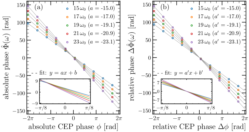
Figure S6: Numerical Simulations. Relative Spectral Phase Retrieval: (a) Absolute spectral phase of the dipole acceleration $\Phi_{1}(\omega)=\arg_{\omega}\mathcal{F}\left[\ddot{d}_{z}(t)\right](\omega)$ for different harmonic frequencies, $\omega=(2k\!+\!1)\omega_{0}$, as a function of the absolute CEP of the IR field in Arm 1 (in the absence of IR 2). $\Phi_{1}(\omega/\omega_{0})$ exhibits a linear behaviour $y=ax+b$ as a function of the IR CEP with a slope $a$ that corresponds to the harmonic order. (b) Spectral phase of the interfering HHG harmonic signal arising from both arms, corresponding to the phase in the interference fringes shown in Fig. S5 as a function of the relative CEP phase of the IR fields acting on the samples in arms 1 and 2. It corresponds to the relative spectral phase $\Delta\Phi(\omega)\equiv\Phi^{(1)}_{dip}(\omega)-\Phi^{(2)}_{dip}(\omega)$ appearing in (S25c).

The quantity $\langle S_{D}\rangle(\boldsymbol{r}_{d},\omega)$ in (S25) describes the interfering HHG radiation signal arising from both arms and depends parametrically on $\Delta\phi$, i.e., $\langle S_{D}\rangle(\boldsymbol{r}_{d},\omega)=\langle S_{D}\rangle(\boldsymbol{r}_{d},\omega;\Delta\phi)$. To extract the phase from $\langle S_{D}\rangle(\boldsymbol{r}_{d},\omega;\Delta\phi)$, for each $\Delta\phi$ we introduce the transformation,

$$\hat{G}_{\Delta\phi}\big{[}\langle S_{D}\rangle(\boldsymbol{r}_{d},\omega;\Delta\phi)\big{]}(\omega_{j})=\int dZ\,\,\langle S_{D}\rangle(\boldsymbol{r}_{d},\omega;\Delta\phi)\,e^{-i\omega_{j}\,Z}\,,$$ (S27a)

with $$Z\equiv\Omega_{Z}\,\delta z/c \delta z\equiv z_{2}-z_{1} z- x_{\alpha}=y_{\alpha}=0 \alpha=1,2 n_{1}(\omega)=n_{2}(\omega)=1 \langle S_{D}\rangle(\boldsymbol{r}_{d},\omega;\Delta\phi) \omega=\omega_{j} \Delta\phi$$ and where is relative position of the samples along the axis in Fig. S4. As stated above, we have assumed that for both , and , see main text. The phase of at fixed and relative CEP is then given by,

$$\Delta\hat{\Phi}(\omega_{j};\Delta\phi)=\arg\big{\{}\hat{G}_{\Delta\phi}[\langle S_{D}\rangle(\boldsymbol{r}_{d},\omega;\Delta\phi)](\omega_{j})\big{\}}\,.$$ (S27b)

Figure S6 is repeated from the main text here for simplicity. Panel (a) shows the absolute spectral phase of the Fourier transform of the dipole acceleration,$\hat{\ddot{d}}(\omega)$, in arm $\alpha=2$ for the harmonics $(2j+1)\omega_{0}$ as a function of the absolute CEP phase of the IR pulse acting on a single-atom in the sample $\alpha=2$. A linear fit $y=ax+b$ shows that, at the atomic level, the absolute spectral phase of a given high-order harmonic $\omega_{2k+1}=(2k+1)\omega_{0}$ exhibits a linear dependence on the absolute CEP phase of the IR pulse, whereby the slope $a$ in Fig. S6(a) coincides with the harmonic order $(2k+1)$.

On the other hand, Fig. S6(b) shows the spectral phase of the interfering HHG radiation signal extracted from $\langle S_{D}\rangle(\boldsymbol{r}_{d},\omega;\Delta\phi)$ using (S27). This is, the phase of the the “macroscopic”, time-averaged Poynting vector given by (S25) for which we have used the macroscopic, i.e., volume-averaged, electric fields arising from both arms $(\alpha=1,2)$ that interfere at a common point in the detector. In Fig. S6(b) the horizontal axis correspond to the relative CEP of the IR pulses acting on samples $\alpha=1$ and $\alpha=2$. It is to note that from (S25c), the phase of $\langle S_{D}\rangle(\boldsymbol{r}_{d},\omega;\Delta\phi)$ corresponds to the relative spectral phases of the atomic dipoles $\Delta\phi_{dip}(\omega)=\phi^{(1)}_{dip}(\omega)-\phi^{(2)}_{dip}(\omega)$. For a relative CEP $\Delta\phi=0$, we obtain a value of $\Delta\hat{\Phi}(\omega_{j})=0$, see inset in Eq. S5(b). For comparison, absolute phase information are shown in the inset of Fig. S5(a). Numerical simulations are thus in good agreement with the experimental measurements reported in Fig. (2) in the main text, showing the linear phase evolution of harmonics 15-21 generated in Ar as a function of fundamental phase difference.

As an alternative approach to (S27), relative spectral phase information can also be extracted by using a variational approach on the quantity $\langle S_{D}\rangle(\boldsymbol{r}_{d},\omega;\Delta\phi)$,

$$\delta\langle S_{D}\rangle(\boldsymbol{r}_{d},\omega;\Delta\phi)\equiv\langle S_{D}\rangle(\boldsymbol{r}_{d},\omega;\Delta\phi+d(\Delta\phi))-\langle S_{D}\rangle(\boldsymbol{r}_{d},\omega;\Delta\phi)=0$$ (S28a)

After Taylor expansion of the first term in the RHS of the above expression to the first order, we obtain the extremum condition $$\omega\delta zd\Omega_{z}/c+\Delta\hat{\Phi}^{\prime}(\omega,\Delta\phi)=0 \Delta\hat{\Phi}^{\prime}\equiv d(\Delta\hat{\Phi})/d(\Delta\phi) d\Delta\hat{\Phi}/d(\Delta\phi) \omega$$ with , where is precisely the quantity of interest, i.e., the slope of the (linear) functions shown in Fig. S6(b) at a fixed frequency . This gives an alternative way to extract the relative phase information, namely

$$\Delta\Phi^{\prime}\equiv(\partial/\partial(\Delta\phi))\,\Delta{\Phi}(\omega,\Delta\phi)=-\dfrac{\omega}{c}\delta_{z}\,\,\dfrac{d\Omega_{z}}{d(\Delta\Phi)}$$ (S28b)

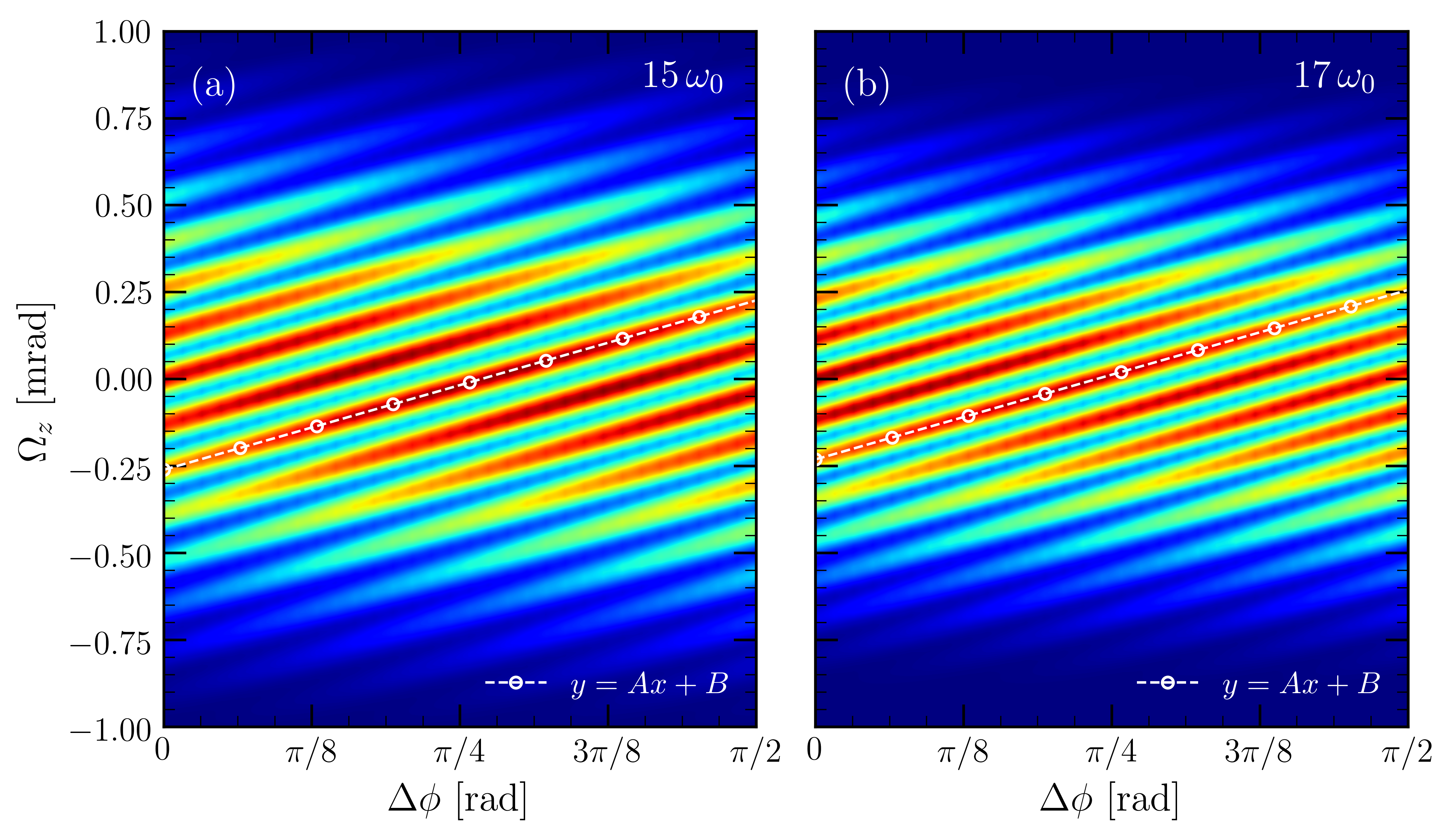
Figure S7: Numerical Simulations: (a) Surface projection of $\langle S_{D}\rangle(\boldsymbol{r}_{d},\omega;\Delta\phi)$ as a function of the divergence angle $\Omega_{Z}$ and relative CEP $\Delta\phi$ for the harmonics $15\omega_{0}$ (a) and $17\omega_{0}$ (b). Dashed-white lines correspond to isolines within a small surface area $\delta^{2}A=d\Omega_{Z}\times d\Delta\phi$. The slopes $d(\Omega_{z})/d(\Delta\phi)$ along the parallel lines are used to extract the spectral phase information following (S28).

where the function $d\Omega_{z}/d(\Delta\Phi)$ appearing in the RHS in (S28b) corresponds to the isolines of the surface projection of $\langle S_{D}\rangle(\boldsymbol{r}_{d},\omega;\Delta\phi)$ on the $(\Omega_{z}-\Delta\phi)$ plane for a fixed value of $\omega$. Figure S7 shows this projection for some fixed harmonics $\omega$. In the projection plane, $\Omega_{Z}$ can be viewed a linear function of the relative CEP $\Delta\phi$. The slope $d(\Omega_{z})/d(\Delta\phi)$ denoted by $A$ in Fig. S7 can be evaluated numerically following the isolines within a small surface area $\delta^{2}A=d\Omega_{Z}\times d\Delta\phi$. The slope of the relative spectral phase is then given by $\Delta\hat{\Phi}(\omega)/d(\Delta\phi)=-\dfrac{\omega}{c}\,\delta z\,A$ for each $\Delta\phi$. Numerical evaluation of the slopes $d(\Omega_{z})/d(\Delta\phi)$ along e.g., the white-dashed lines in Fig. S7 results in a constant value for $d(\Omega_{z})/d(\Delta\phi)$ at all $\Delta\phi$ and depend only on the harmonic considered. The multiplicative factor $\omega\delta z/c$ in the RHS of Eq. (S28b) ultimately gives the slope of the spectral phase of $\langle S_{D}\rangle(\boldsymbol{r}_{d},\omega;\Delta\phi)$ as a function of $\Delta\phi$, which again coincides with the harmonic order, i.e., the numerical values denotes as $a\prime$ in Fig. S6(b). Geometry parameters: same as in Fig. S5 but $z_{\alpha}=\pm 20\,\mu\text{m}$.

References

- [1] P. M. Paul, E. S. Toma, P. Breger, G. Mullot, F. Auge, P. Balcou, H. G. Muller, and P. Agostini, “Observation of a train of attosecond pulses from high harmonic generation,” \JournalTitleScience 292, 1689–1692 (2001).
- [2] K. Oguri, H. Mashiko, T. Ogawa, Y. Hanada, H. Nakano, and H. Gotoh, “Sub-50-as isolated extreme ultraviolet continua generated by 1.6-cycle near-infrared pulse combined with double optical gating scheme,” \JournalTitleApplied Physics Letters 112, 181105 (2018).
- [3] M. Lewenstein, P. Balcou, M. Y. Ivanov, A. L’huillier, and P. B. Corkum, “Theory of high-harmonic generation by low-frequency laser fields,” \JournalTitlePhysical Review A 49, 2117 (1994).
- [4] A. L’Huillier and P. Balcou, “High-order harmonic generation in rare gases with a 1-ps 1053-nm laser,” \JournalTitlePhysical Review Letters 70, 774 (1993).
- [5] J. L. Krause, K. J. Schafer, and K. C. Kulander, “High-order harmonic generation from atoms and ions in the high intensity regime,” \JournalTitlePhysical Review Letters 68, 3535 (1992).
- [6] I. Orfanos, I. Makos, I. Liontos, E. Skantzakis, B. Förg, D. Charalambidis, and P. Tzallas, “Attosecond pulse metrology,” \JournalTitleApl Photonics 4, 080901 (2019).
- [7] V. I. Ritus, “Quantum effects of the interaction of elementary particles with an intense electromagnetic field,” \JournalTitleJ. Sov. Laser Res. 6, 497–617 (1985).
- [8] A. Di Piazza, C. Müller, K. Z. Hatsagortsyan, and C. H. Keitel, “Extremely high-intensity laser interactions with fundamental quantum systems,” \JournalTitleRev. Mod. Phys. 84, 1177–1228 (2012).
- [9] T. N. Wistisen, A. Di Piazza, H. V. Knudsen, and U. I. Uggerhøj, “Experimental evidence of quantum radiation reaction in aligned crystals,” \JournalTitleNat. Commun. 9, 1–6 (2018).
- [10] K. Poder, M. Tamburini, G. Sarri, A. Di Piazza, S. Kuschel, C. D. Baird, K. Behm, S. Bohlen, J. M. Cole, D. J. Corvan, M. Duff, E. Gerstmayr, C. H. Keitel, K. Krushelnick, S. P. Mangles, P. McKenna, C. D. Murphy, Z. Najmudin, C. P. Ridgers, G. M. Samarin, D. R. Symes, A. G. Thomas, J. Warwick, and M. Zepf, “Experimental Signatures of the Quantum Nature of Radiation Reaction in the Field of an Ultraintense Laser,” \JournalTitlePhys. Rev. X 8, 031004 (2018).
- [11] M. Lewenstein, N. Baldelli, U. Bhattacharya, J. Biegert, M. F. Ciappina, U. Elu, T. Grass, P. T. Grochowski, A. Johnson, T. Lamprou, A. S. Maxwell, A. Ordóñez, E. Pisanty, J. Rivera-Dean, P. Stammer, I. Tyulnev, and P. Tzallas, “Attosecond Physics and Quantum Information Science,” \JournalTitlearXiv (2022).
- [12] H. P. Yuen and V. W. S. Chan, “Noise in homodyne and heterodyne detection,” \JournalTitleOptics Letters 8, 177 (1983).
- [13] B. Kühn and W. Vogel, “Unbalanced Homodyne Correlation Measurements,” \JournalTitlePhysical Review Letters 116, 163603 (2016).
- [14] G. Roumpos and S. T. Cundiff, “Multichannel homodyne detection for quantum optical tomography,” \JournalTitleJournal of the Optical Society of America B 30, 1303 (2013).
- [15] A. Mandal, M. S. Sidhu, J. M. Rost, T. Pfeifer, and K. P. Singh, “Attosecond delay lines: Design, characterization and applications,” \JournalTitleThe European Physical Journal Special Topics pp. 1–19 (2021).
- [16] J. Köhler, M. Wollenhaupt, T. Bayer, C. Sarpe, and T. Baumert, “Zeptosecond precision pulse shaping,” \JournalTitleOptics Express 19, 11638–11653 (2011).
- [17] R. Zerne, C. Altucci, M. Bellini, M. B. Gaarde, T. Hänsch, A. L’Huillier, C. Lyngå, and C.-G. Wahlström, “Phase-locked high-order harmonic sources,” \JournalTitlePhysical Review Letters 79, 1006 (1997).
- [18] Y. Meng, C. Zhang, C. Marceau, A. Y. Naumov, P. Corkum, and D. Villeneuve, “Octave-spanning hyperspectral coherent diffractive imaging in the extreme ultraviolet range,” \JournalTitleOptics Express 23, 28960–28969 (2015).
- [19] G. Jansen, D. Rudolf, L. Freisem, K. Eikema, and S. Witte, “Spatially resolved fourier transform spectroscopy in the extreme ultraviolet,” \JournalTitleOptica 3, 1122–1125 (2016).
- [20] L.-M. Koll, L. Maikowski, L. Drescher, M. J. Vrakking, and T. Witting, “Phase-locking of time-delayed attosecond xuv pulse pairs,” \JournalTitleOptics Express 30, 7082–7095 (2022).
- [21] J. Tross, G. Kolliopoulos, and C. A. Trallero-Herrero, “Self referencing attosecond interferometer with zeptosecond precision,” \JournalTitleOptics Express 27, 22960–22969 (2019).
- [22] G. R. Harrison, T. Saule, B. Davis, and C. A. Trallero-Herrero, “Increased phase precision of spatial light modulators using irrational slopes: application to attosecond metrology,” \JournalTitleApplied Optics 61, 8873–8879 (2022).
- [23] T. Kaneyasu, Y. Hikosaka, S. Wada, M. Fujimoto, H. Ota, H. Iwayama, and M. Katoh, “Time domain double slit interference of electron produced by XUV synchrotron radiation,” \JournalTitleSci. Reports 2023 131 13, 1–8 (2023).
- [24] A. Gorlach, O. Neufeld, N. Rivera, O. Cohen, and I. Kaminer, “The quantum-optical nature of high harmonic generation,” \JournalTitleNature communications 11, 1–11 (2020).
- [25] J. Troß, X. Ren, V. Makhija, S. Mondal, V. Kumarappan, and C. A. Trallero-Herrero, “N 2 HOMO-1 orbital cross section revealed through high-order-harmonic generation,” \JournalTitlePhysical Review A 95, 033419 (2017).
- [26] Z. Rodnova, T. Saule, R. Sadlon, E. McManus, N. May, X. Yu, S. Shahbazmohamadi, and C. Trallero, “Generation and control of phase-locked Bessel beams with a persistent non-interfering region,” \JournalTitleJournal of the Optical Society of America B 37, 3179–3183 (2020).
- [27] M. Davino, A. Summers, T. Saule, J. Tross, E. McManus, B. Davis, and C. Trallero-Herrero, “Higher-order harmonic generation and strong field ionization with bessel–gauss beams in a thin jet geometry,” \JournalTitleJOSA B 38, 2194–2200 (2021).
- [28] H. Wang, Y. Xu, S. Ulonska, J. S. Robinson, P. Ranitovic, and R. A. Kaindl, “Bright high-repetition-rate source of narrowband extreme-ultraviolet harmonics beyond 22 ev,” \JournalTitleNature communications 6, 1–7 (2015).
- [29] D. Wilson, M. Ivanov, G. Tempea, A. Labranche, A. Ramirez, F. Legare, C. Paradis, A. Hage, T. Mans, C. Trallero, and B. E. Schmidt, “10mJ Hollow-Core Fiber operation at 250W average power with 90% efficiency,” in 2022 Conference on Lasers and Electro-Optics, CLEO 2022 - Proceedings, (Optica Publishing Group, 2022), p. SM3O.6.
- [30] S. Hädrich, M. Krebs, A. Hoffmann, A. Klenke, J. Rothhardt, J. Limpert, and A. Tünnermann, “Exploring new avenues in high repetition rate table-top coherent extreme ultraviolet sources,” \JournalTitleLight: Science & Applications 4, e320–e320 (2015).
- [31] G. Zhu, D. Whitehead, W. Perrie, O. Allegre, V. Olle, Q. Li, Y. Tang, K. Dawson, Y. Jin, S. Edwardson et al., “Investigation of the thermal and optical performance of a spatial light modulator with high average power picosecond laser exposure for materials processing applications,” \JournalTitleJournal of Physics D: Applied Physics 51, 095603 (2018).
- [32] J. J. Kaakkunen, I. Vanttaja, and P. Laakso, “Fast micromachining using spatial light modulator and galvanometer scanner with infrared pulsed nanosecond fiber laser,” \JournalTitleJournal of Laser Micro Nanoengineering 9, 37 (2014).
- [33] S. Carbajo and K. Bauchert, “Power handling for lcos spatial light modulators,” in Laser Resonators, Microresonators, and Beam Control XX, vol. 10518 (SPIE, 2018), pp. 282–290.
- [34] A. Mair, A. Vaziri, G. Weihs, and A. Zeilinger, “Entanglement of the orbital angular momentum states of photons,” \JournalTitleNature 412, 313–316 (2001).
- [35] R. Fickler, G. Campbell, B. Buchler, P. K. Lam, and A. Zeilinger, “Quantum entanglement of angular momentum states with quantum numbers up to 10,010,” \JournalTitleProceedings of the National Academy of Sciences of the United States of America 113, 13642–13647 (2016).
- [36] F. Kong, C. Zhang, F. Bouchard, Z. Li, G. G. Brown, D. H. Ko, T. J. Hammond, L. Arissian, R. W. Boyd, E. Karimi, and P. B. Corkum, “Controlling the orbital angular momentum of high harmonic vortices,” \JournalTitleNature Communications 8 (2017).
- [37] J. Troß and C. A. Trallero-Herrero, “High harmonic generation spectroscopy via orbital angular momentum,” \JournalTitleThe Journal of Chemical Physics 151, 084308 (2019).
- [38] A. D. Shiner, C. Trallero-Herrero, N. Kajumba, H.-C. Bandulet, D. Comtois, F. Légaré, M. Giguère, J.-C. Kieffer, P. B. Corkum, and D. M. Villeneuve, “Wavelength scaling of high harmonic generation efficiency.” \JournalTitlePhysical Review Letters 103, 073902 (2009).
- [39] A. Shiner, C. Trallero-Herrero, N. Kajumba, B. Schmidt, J. Bertrand, K. T. Kim, H.-C. Bandulet, D. Comtois, J.-C. Kieffer, D. Rayner, P. Corkum, F. Légaré, and D. Villeneuve, “High harmonic cutoff energy scaling and laser intensity measurement with a 1.8 m laser source,” \JournalTitleJournal of Modern Optics 60, 1458–1465 (2013).
- [40] B. Shore and K. Kulander, “Generation of optical harmonics by intense pulses of laser radiation,” \JournalTitleJournal of Modern Optics 36, 857–875 (1989).
- [41] L. Greenman, P. J. Ho, S. Pabst, E. Kamarchik, D. A. Mazziotti, and R. Santra, “Implementation of the time-dependent configuration-interaction singles method for atomic strong-field processes,” \JournalTitlePhys. Rev. A 82, 023406 (2010).
- [42] C. L. Smallwood, J. P. Hinton, C. Jozwiak, W. Zhang, J. D. Koralek, H. Eisaki, D.-H. Lee, J. Orenstein, and A. Lanzara, “Tracking Cooper pairs in a cuprate superconductor by ultrafast angle-resolved photoemission.” \JournalTitleScience 336, 1137 (2012).
- [43] C. Corder, P. Zhao, J. Bakalis, X. Li, M. D. Kershis, A. R. Muraca, M. G. White, and T. K. Allison, “Ultrafast extreme ultraviolet photoemission without space charge,” \JournalTitleStruct. Dyn. 5, 054301 (2018).
- [44] E. J. Sie, T. Rohwer, C. Lee, and N. Gedik, “Time-resolved XUV ARPES with tunable 24–33 eV laser pulses at 30 meV resolution,” \JournalTitleNat. Commun. 10, 1–11 (2019).
- [45] J. Berakdar, “Emission of correlated electron pairs following single-photon absorption by solids and surfaces,” \JournalTitlePhysical Review B - Condensed Matter and Materials Physics 58, 9808–9816 (1998).
- [46] F. Mahmood, T. Devereaux, P. Abbamonte, and D. K. Morr, “Distinguishing finite-momentum superconducting pairing states with two-electron photoemission spectroscopy,” \JournalTitlePhysical Review B 105, 064515 (2022).
- [47] J. C. Baggesen and L. B. Madsen, “On the dipole, velocity and acceleration forms in high-order harmonic generation from a single atom or molecule,” \JournalTitleJournal of Physics B: Atomic, Molecular and Optical Physics 44, 115601 (2011).
- [48] M. Born and E. Wolf, Principles of Optics: 60th Anniversary Edition (Cambridge University Press, 2019), 7th ed.
- [49] B. Saleh and M. Teich, Fundamentals of Photonics, 3rd Edition (2019).
- [50] A. E. Siegman, Lasers / Anthony E. Siegman (University Science Books Mill Valley, Calif, 1986).