FineMorphs: affine-diffeomorphic sequences for regression

Abstract.

A multivariate regression model of affine and diffeomorphic transformation sequences—FineMorphs—is presented. Leveraging concepts from shape analysis, model states are optimally “reshaped” by diffeomorphisms generated by smooth vector fields during learning. Affine transformations and vector fields are optimized within an optimal control setting, and the model can naturally reduce (or increase) dimensionality and adapt to large datasets via suboptimal vector fields. An existence proof of solution and necessary conditions for optimality for the model are derived. Experimental results on real datasets from the UCI repository are presented, with favorable results in comparison with state-of-the-art in the literature and densely-connected neural networks in TensorFlow.

1. Introduction

We present FineMorphs—an affine-diffeomorphic sequence model for multivariate regression. Our approach combines arbitrary sequences of affine and diffeomorphic transformations with a training algorithm using concepts from optimal control. Predictors, estimated responses, and states in between are transformed or “reshaped” via diffeomorphisms of their respective ambient spaces, in an optimal way to facilitate learning.

Recall that diffeomorphisms of an open subset $M$ of a Euclidean space $\mathbb{R}^{d}$ (where we will typically take $M=\mathbb{R}^{d}$) are one-to-one, invertible, $C^{1}$ transformations mapping $M$ onto itself that have $C^{1}$ inverse. (If $C^{1}$ is replaced by $C^{0}$, one speaks of homeomorphisms.) Because diffeomorphisms form a group, arbitrary large deformations can be generated via the composition of many small ones, making them natural objects to utilize within a feed forward setting. In the limit of infinite compositions of transformations that differ infinitesimally from the identity, one finds the classical representation of diffeomorphisms as flows associated to ordinary differential equations (ODEs).

Several papers have recently explored the possibility of using homeomorphic or diffeomorphic transformations within feed-forward machine learning models. Discrete invertible versions of the ResNet architecture (He et al., 2016) were proposed as “normalizing flows” in Rezende and Mohamed (2015) (see Kobyzev et al. (2020) for a recent review), and extended to a time-continuous form in Chen et al. (2018); Rousseau et al. (2019); Dupont et al. (2019). Continuous-time optimal control as a learning principle was proposed in Weinan (2017); Owhadi (2023); Ganaba (2021). Applications of deep residual neural networks (NNs) to the large deformation diffeomorphic metric mapping (LDDMM) framework of shape analysis have recently been explored (Amor et al., 2023; Wu and Zhang, 2023) as well as sub-Riemannian landmark matching as time-continuous NNs (Jansson and Modin, 2022).

A direct formalization of the diffeomorphic learning approach was proposed in Younes (2020). While most flow-based learning approaches build dynamical systems that are adapted to NN implementations, diffeomorphic learning is presented as a non-parametric penalized regression problem, parametrized by a diffeomorphism of the data space. The penalty is specified as a Riemannian metric on the diffeomorphism group, in a framework directly inspired from shape analysis (Younes, 2010). When applied to finite training data, the method reduces to a finite-, albeit large-, dimensional problem involving reproducing kernels (see Section 6). Shape analysis methods were also introduced for dimensionality reduction in Walder and Schölkopf (2009). Similar models were used combined with a shooting formulation for the comparison of geodesics in Vialard et al. (2020).

In this paper, we provide three extensions to the approach in Younes (2020), with existence proof of solution and derivation of necessary conditions for optimality. First, we extend the single diffeomorphic layer sequence approach to arbitrary affine-diffeomorphic sequences, providing a natural framework for automated data scaling as well as dimensionality reduction. Second, we extend the model from classification to regression. In particular, we consider vector regression predictors of the form

(1) $$x\in\mathbb{R}^{d_{X}}\mapsto A_{m}\circ\varphi_{m}\circ A_{m-1}\circ\cdots\circ\varphi_{1}\circ A_{0}(x)\in\mathbb{R}^{d_{Y}},$$

where $A_{q},$ $q=0,\dots,m,$ are affine transformations from $\mathbb{R}^{{d}_{q}}$ to $\mathbb{R}^{{d}_{q+1}},$ and $\varphi_{q},$ $q=1,\dots,m,$ are diffeomorphisms on $\mathbb{R}^{d_{q}}.$ In this model, a $d_{Y}$-dimensional output variable is predicted by the transformation of a $d_{X}$-dimensional input through an arbitrary number and order of arbitrary affine and diffeomorphic transformations. Third, we extend the approach to include a more general sub-optimal vector fields setting to train diffeomorphisms on a subset of the training data, providing a natural framework for dataset (and model) reduction in the case of very large datasets. Combined with a GPU implementation, this allows for experiments on datasets beyond smaller-sized, simulated datasets to real-world data with larger, more realistic dimensions and sizes.

We test our diffeomorphic regression models on real datasets from the UCI repository (Dua and Graff, 2017), with favorable results in comparison with the literature and with densely-connected NNs (DNNs) in TensorFlow (Abadi et al., 2015). We note improved performance with multiple sequential diffeomorphic modules with decreasing kernel sizes as well as a robustness of our models to “out-of-distribution” testing. For the largest dataset in our experiments, in both dimensionality and number size, our model reduces dimensionality through affine transformations and reduces number through sub-optimal vector fields, with a significant decrease in run-time and good predictive results in comparison with the literature and DNNs.

Notation

For our multivariate regression setting, $X:\Omega\to\mathbb{R}^{d_{X}}$ is the predictor variable and $Y:\Omega\to\mathbb{R}^{d_{Y}}$ is the response. The training dataset is denoted

$${\mathcal{T}_{0}=(x_{1},y_{1},\dots,x_{N},y_{N}).}$$

The training predictors are $\boldsymbol{x}=(x_{1},\dots,x_{N})\in(\mathbb{R}^{d_{X}})^{N}$ and training responses are $\boldsymbol{y}=(y_{1},\dots,y_{N})\in(\mathbb{R}^{d_{Y}})^{N}$. We define the operator $\iota_{j}:\mathbb{R}^{d}\to\mathbb{R}^{d+j}$, where $\iota_{j}(x)$ appends $j$ zero coordinates to $x$, and the operator $\pi_{j}:\mathbb{R}^{d}\to\mathbb{R}^{d-j}$, where $\pi_{j}(x)$ removes the last $j$ coordinates from $x.$ For matrix notation, if $k,l$ are two integers, $\mathcal{M}_{k,l}(\mathbb{R})$ is the space of all $k\times l$ real matrices, reducing to $\mathcal{M}_{k}(\mathbb{R})$ for square $k\times k$ real matrices. The $d\times d$ identity matrix is denoted $\mathrm{I}_{d}.$ When applied to vectors and matrices, the norm $\|\cdot\|$ is the Euclidean and Frobenius norm, respectively. For time-dependent vector fields

$$v:\mathbb{R}\times\mathbb{R}^{d} \rightarrow\mathbb{R}^{d}$$

$$(t,x) \mapsto v(t,x)$$

we will denote by $v$ the mapping ${t\mapsto v(t),}$ where $v(t)$ is the time-indexed vector field $x\mapsto v(t,x).$ In particular, the time-dependent vector fields $v$ in the Bochner spaces $L^{2}(I,V)$ will represent the mapping

$$t\in I\mapsto v(t)\in V,$$

where $V$ is a Hilbert space.

2. Model

We consider the following regression model approximating $Y$ by $f(X)$, in which we complete (1) by possibly padding zeros in input and removing coordinates in output,

$$f:x\in\mathbb{R}^{d_{X}}\mapsto\pi_{r}\left(A_{m}\circ\varphi_{m}\circ A_{m-1}\circ\cdots\circ\varphi_{1}\circ A_{0}(\iota_{s}(x))\right)\in\mathbb{R}^{d_{Y}}.$$

Here, $\iota_{s}$ pads the input with $s$ zeros so that ${d_{0}=d_{X}+s,}$ and $\pi_{r}$ removes the last $r$ coordinates from the model output so that $d_{m+1}=d_{Y}+r$. Advantages of adding “dummy” dimensions are discussed in Section 9. In contrast to the single affine layered approach of standard linear regression, this model alternates $m+1$ affine transformations and $m$ diffeomorphic layers, denoted as A and D modules, respectively, starting and ending with affine modules. For affine modules A${}_{q},$ ${q=0,\dots,m,}$ the corresponding affine transformations are

$${A}_{q}:x\in\mathbb{R}^{{d}_{q}}\mapsto M_{q}x+b_{q}\in\mathbb{R}^{{d}_{q+1}},$$

where ${M_{q}\in\mathcal{M}_{d_{q+1},d_{q}}(\mathbb{R}),}$ ${b_{q}\in\mathbb{R}^{d_{q+1}}.}$ For diffeomorphic modules D${}_{q},$ $q=1,\dots,m,$ the corresponding diffeomorphisms and their domains are $\varphi_{q}$ and $\mathbb{R}^{d_{q}},$ respectively.

The values of $n$ and $r$, and the internal dimensions $d_{1},\ldots,d_{m}$ are parts of the design of the model, i.e., they are user-specified. Given them, the dimensions of the linear operators are uniquely determined, and so are the spaces on which the diffeomorphisms operate. Any module in a sequence with identical input and output dimensions can be set to the identity map, $\mathrm{id}$, which allows for simple definitions of submodels from an initial sequence of modules (obviously, one wants to keep at least one A module and at least one D module free to optimize by the system). The flexibility of assigning module dimensions as well as arbitrary modules to the identity generalizes our model from a simple and fixed alternating sequence to an arbitrary sequence of arbitrary affine and diffeomorphic transformations. In this setting, affine modules can provide not only useful data scaling prior to diffeomorphic transforms but also a natural approach to dimensionality reduction or increase. In the following, the naming convention for sequences includes only non-identity modules, e.g., the sequence of modules A${}_{0},$ D${}_{1},$ A${}_{1},$ D${}_{2},$ A${}_{2},$ D${}_{3},$ and A${}_{3},$ where A₁ and D₃ are identities, is denoted ADDAA. For sequence names containing repetitive module or module subsequence elements, we further adopt a simplified notation superscripting the repetition, e.g., ADDAA can be expressed as AD²A${}^{2},$ and sequence ADAD$\cdots$A with x sequential AD module pairs before the final A can be denoted as (AD)^xA. Several sequence examples are illustrated in Figure 1, including the smallest possible sequences that can be represented in our model, DA and AD.

Figure 1. Standard linear regression (top) followed by four example transformation sequences that can be operated by the FineMorphs model, with naming convention (from top to bottom): A, DA, AD, DADA or (DA)${}^{2},$ and ADDAA or AD²A² (A: affine module; D: diffeomorphic module). Identity modules are omitted.

3. Objective Function

Learning is implemented by minimizing the objective function

$$\sum_{q=1}^{m}d_{V_{q}}(\mathrm{id},\varphi_{q})^{2}+\lambda\sum_{q=0}^{m}U_{q}({A}_{q})+\frac{1}{\sigma^{2}}\sum_{k=1}^{N}\Gamma_{k}(\pi_{r}({A}_{m}\circ\varphi_{m}\circ{A}_{m-1}\circ\cdots\circ\varphi_{1}\circ{A}_{0}(\iota_{s}(x_{k}))))$$

over $\varphi_{1},\dots,\varphi_{m},{A}_{0},\dots,{A}_{m}.$ The objective function combines an optimal deformation cost $d_{V_{q}},$ an affine cost $U_{q},$ and a standard loss function or endpoint cost $\Gamma_{k}.$ In our setting, $d_{V_{q}}$ is a Riemannian distance in a group of diffeomorphisms of $\mathbb{R}^{d_{q}}$ described in Section 4, $U_{q}$ is a ridge regularization function

$$U_{q}({A})=\left\|M\right\|^{2}=\mathrm{trace}(M^{T}M)$$

for affine transformations ${A}:\mathbb{R}^{d_{q}}\rightarrow\mathbb{R}^{d_{q+1}}$ of the form ${A}(x)=Mx+b,$ ${M\in\mathcal{M}_{d_{q+1},d_{q}}(\mathbb{R}),}$ ${b\in\mathbb{R}^{d_{q+1}},}$ and $\Gamma_{k}$ is a squared error loss function

$$\Gamma_{k}(\cdot)=\left\|y_{k}-(\cdot)\right\|^{2}$$

for comparison of experimental responses with model predictions.

4. Distance over Diffeomorphisms

Spaces of diffeomorphisms are defined as follows. Let $\mathrm{\textbf{B}}_{p}=C_{0}^{p}(\mathbb{R}^{d},\mathbb{R}^{d})$ denote the space of $C^{p}$ vector fields on $\mathbb{R}^{d}$ that tend to zero (together with their first $p$ derivatives) at infinity. This is a Banach space for the norm

$$\left\|f\right\|_{p,\infty}=\max_{0\leq k\leq p}\left\|d^{k}f\right\|_{\infty},$$

where $\left\|\,\cdot\,\right\|_{\infty}$ denotes the usual supremum norm. Let $V$ denote a Hilbert space of vector fields on $\mathbb{R}^{d},$ continuously embedded in $\mathrm{\textbf{B}}_{p}$ for some $p\geq 1,$ so that there exists a $C>0$ such that

$$\left\|f\right\|_{p,\infty}\leq C\left\|f\right\|_{V},$$

for all $f\in V,$ where $\left\|\cdot\right\|_{V}$ is the Hilbert norm on $V$ with inner product $\langle\cdot,\cdot{\rangle}_{V}.$

Diffeomorphisms can be generated as flows of ODEs associated with time-dependent elements of $V.$ Let $\mathcal{H}$ denote the Hilbert space ${L^{2}([0,1],V)}$ of time-dependent vector fields, so that ${v\in\mathcal{H}}$, if and only if ${v(t)\in V}$ for $t\in[0,1]$, $v$ is measurable and

$$\|v\|_{\mathcal{H}}^{2}=\int_{0}^{1}\|v(t)\|_{V}^{2}dt<\infty,$$

where $\|\cdot\|_{\mathcal{H}}$ denotes the norm on $\mathcal{H}$ with inner product $\langle\cdot,\cdot{\rangle}_{\mathcal{H}}$. Then the ODE

$$\partial_{t}y(t)=v(t)(y(t))$$

has a unique solution over $[0,1]$ given any initial condition $y(0)=x.$ The flow of the ODE is the function

$${\boldsymbol{\varphi}}_{v}:(t,x)\mapsto y(t),$$

where $y(t)$ is the solution starting at $x,$ after $t$ units of time. This function is the unique flow of $\mathbb{R}^{d}$-diffeomorphisms satisfying the dynamical system

$$\partial_{t}{\boldsymbol{\varphi}}_{v}(t,x) =v(t)({\boldsymbol{\varphi}}_{v}(t,x))$$

$${\boldsymbol{\varphi}}_{v}(0,x) =x$$

over $t\in[0,1].$ We will often write ${\boldsymbol{\varphi}}_{v}(t)$ for the time-indexed function $x\mapsto{\boldsymbol{\varphi}}_{v}(t,x)$ satisfying

$$\partial_{t}{\boldsymbol{\varphi}}_{v}(t) =v(t)\circ{\boldsymbol{\varphi}}_{v}(t),\quad t\in[0,1]$$

$${\boldsymbol{\varphi}}_{v}(0) =\mbox{id}.$$

The set of diffeomorphisms that can be generated in such a way forms a group denoted $\mathrm{Diff}_{V},$ such that a flow path associated with some $v\in V$ is a curve on $\mathrm{Diff}_{V}$. Let $\frac{1}{2}\|v(t)\|_{V}^{2}$ denote the kinetic energy associated with the flow’s velocity at time $t$ along this curve. Given $\psi\in\mathrm{Diff}_{V}$, we define the optimal deformation cost from $\mathrm{id}$ to $\psi$ as the minimal kinetic energy among all curves between $\mathrm{id}$ and $\psi$ on $\mathrm{Diff}_{V}$, i.e., the minimum of $\int_{0}^{1}\|v(t)\|_{V}^{2}dt$ over all ${v\in\mathcal{H}}$ such that ${\boldsymbol{\varphi}}_{v}(1)=\psi.$ A right-invariant distance $d_{V}(\cdot,\cdot)$ can then be defined on $\mathrm{Diff}_{V}$. Given $\psi,\psi^{\prime}\in\mathrm{Diff}_{V},$ ${d_{V}(\psi,\psi^{\prime})=d_{V}(\mathrm{id},\psi^{\prime}\circ\psi^{-1})}$ and

$$d_{V}(\mathrm{id},\psi)^{2}=\min_{v\in\mathcal{H}}\left\{\int_{0}^{1}\|v(t)\|_{V}^{2}dt:{\boldsymbol{\varphi}}_{v}(1)=\psi\right\}\,.$$

In our setting of $m$ distinct D modules, we assume for each D_q module the corresponding Hilbert space $V_{q}$ of vector fields on $\mathbb{R}^{d_{q}}$ and Hilbert space ${L^{2}([0,1],V_{q})}$ denoted $\mathcal{H}_{q},$ and let the time-dependent vector fields ${v_{q}\in\mathcal{H}_{q}}$ generate the corresponding $\mathrm{Diff}_{V_{q}}$ space of diffeomorphisms. Our optimal deformation cost can then be expressed in terms of the vector fields as

$$\sum_{q=1}^{m}d_{V_{q}}(\mathrm{id},\varphi_{q})^{2}=\sum_{q=1}^{m}\min_{v_{q}\in\mathcal{H}_{q}}\left\{\int_{0}^{1}\|v_{q}(t)\|_{V_{q}}^{2}dt:{\boldsymbol{\varphi}}_{v_{q}}(1)=\varphi_{q}\right\},$$

and the objective function becomes

(2) $$\begin{split}&\sum_{q=1}^{m}\int_{0}^{1}\|v_{q}(t)\|_{V_{q}}^{2}dt+\lambda\sum_{q=0}^{m}U_{q}({A}_{q})\\ &\qquad\quad\quad+\frac{1}{\sigma^{2}}\sum_{k=1}^{N}\Gamma_{k}(\pi_{r}({A}_{m}\circ{\boldsymbol{\varphi}}_{v_{m}}(1)\circ{A}_{m-1}\circ\cdots\circ{\boldsymbol{\varphi}}_{v_{1}}(1)\circ{A}_{0}(\iota_{s}(x_{k}))))\end{split}$$

minimized over ${A}_{0},\dots,{A}_{m},$ and $v_{q}\in\mathcal{H}_{q},$ $q=1,\dots,m,$ such that ${\boldsymbol{\varphi}}_{v_{q}}(t)$ satisfies

$$\partial_{t}{\boldsymbol{\varphi}}_{v_{q}}(t) =v_{q}(t)\circ{\boldsymbol{\varphi}}_{v_{q}}(t),\quad t\in[0,1]$$

$${\boldsymbol{\varphi}}_{v_{q}}(0) =\mbox{id}.$$

When the norms on the RKHS’s are translation invariant, a minimizer of this objective function always exists. This is demonstrated in Appendix A.

5. Forward States

We define forward states between modules as $\xi^{0},\zeta^{1},\xi^{1},\zeta^{2},\dots,\xi^{m},\zeta^{m+1},$ as shown in Figure 2, with model input $\xi_{k}^{0}$ and model output $\zeta_{k}^{m+1}.$ The forward states

$$\xi_{k}^{q}={\boldsymbol{\varphi}}_{v_{q}}(1)(\zeta_{k}^{q}),\quad q=1,\dots,m$$

and

$$\zeta_{k}^{q+1}={A}_{q}(\xi_{k}^{q}),\quad q=0,\dots,m$$

are the outputs of the corresponding D_q and A_q modules, respectively, with initialization

$$\xi_{k}^{0}=\iota_{s}(x_{k}).$$

Let

$$z_{k}^{q}(t)={\boldsymbol{\varphi}}_{v_{q}}(t)(\zeta_{k}^{q})$$

represent the time-dependent state in $\mathbb{R}^{d_{q}}$ of module D${}_{q},$ and denote the array of $N$ states as ${\boldsymbol{z}^{q}(\cdot)=(z_{1}^{q}(\cdot),\dots,z_{N}^{q}(\cdot)).}$

6. Kernel Reduction

The assumptions in Section 4 imply that $V_{1},\dots,V_{m}$ are vector-valued RKHSs (Aronszajn, 1950; Wahba, 1990; Joshi and Miller, 2000; Miller et al., 2002; Vaillant et al., 2004; Micchelli and Pontil, 2005). By Riesz’s representation theorem, each $V_{q}$ has an associated matrix-valued kernel function

$$K_{q}:\mathbb{R}^{d_{q}}\times\mathbb{R}^{d_{q}}\rightarrow\mathcal{M}_{d_{q}}(\mathbb{R})$$

that reproduces every function in $V_{q}.$ More precisely, for every $y,a\in\mathbb{R}^{d_{q}}$, there exists a unique element $K_{q}(\cdot,y)a$ of $V_{q}$ such that

$$K_{q}(\cdot,y)a:x\in\mathbb{R}^{d_{q}}\mapsto K_{q}(x,y)a$$

and

$$\langle K_{q}(\cdot,y)a,f{\rangle}_{V_{q}}=a^{T}f(y)$$

for all $f\in V_{q}$. These properties imply

$$\langle K_{q}(\cdot,x)a,K_{q}(\cdot,y)b{\rangle}_{V_{q}}=a^{T}K_{q}(x,y)b$$

and thus symmetry, $K_{q}(y,x)=K_{q}(x,y)^{T}$, and positive semi-definiteness for all $x,y,a,b\in\mathbb{R}^{d_{q}}.$ Conversely, by the Moore–Aronszajn theorem, any matrix-valued kernel that is symmetric and positive semi-definite induces the corresponding vector-valued RKHS of functions reproducible by this kernel.

An RKHS argument similar to the kernel trick used in standard kernel methods can reduce the dimension of our problem as follows. The dependence of our endpoint cost on each vector field $v_{q}(t)$ is through the $N$ trajectories

$$\partial_{t}z_{k}^{q}(t)=v_{q}(t)(z_{k}^{q}(t)),\quad k=1,\dots,N$$

generating the $N$ corresponding endpoints $\zeta_{1}^{m+1},\dots,\zeta_{N}^{m+1}.$ The vector fields minimizing this cost are regularized by the RKHS norm $\|\cdot\|_{V_{q}}$ on their respective spaces $V_{q}.$ By the representer theorem, these minimizers must then take the form

$$v_{q}(t)(\cdot)=\sum_{l=1}^{N}K_{q}(\cdot,z_{l}^{q}(t))a_{l}^{q}(t),$$

where $\boldsymbol{a}^{q}(\cdot)=(a_{1}^{q}(\cdot),\dots,a_{N}^{q}(\cdot))$ are the unknown time-dependent vectors in $\mathbb{R}^{d_{q}}$ to be determined. In this reduced representation, our objective function

$$\begin{split}&\sum_{q=1}^{m}\int_{0}^{1}\sum_{k,l=1}^{N}a_{k}^{q}(t)^{T}K_{q}(z_{k}^{q}(t),z_{l}^{q}(t))a_{l}^{q}(t)dt\\ &\qquad\qquad\qquad\qquad\qquad\quad+\lambda\sum_{q=0}^{m}U_{q}({A}_{q})+\frac{1}{\sigma^{2}}\sum_{k=1}^{N}\Gamma_{k}(\pi_{r}(\zeta_{k}^{m+1}))\end{split}$$

is minimized over $\boldsymbol{a}^{1}(\cdot),\dots,\boldsymbol{a}^{m}(\cdot),$ ${A}_{0},\dots,{A}_{m},$ subject to the system of trajectories and initial conditions

$$\partial_{t}z_{k}^{q}(t) =\sum_{l=1}^{N}K_{q}(z_{k}^{q}(t),z_{l}^{q}(t))a_{l}^{q}(t)$$

$$z_{k}^{q}(0) =\zeta_{k}^{q}={A}_{q-1}(\xi_{k}^{q-1})$$

$$\xi_{k}^{q} =z_{k}^{q}(1)$$

and initialization $\xi_{k}^{0}=\iota_{s}(x_{k}).$ Our learning problem can now be solved as an optimal control problem with a finite dimensional control space.

7. Optimal Control

An optimal control steers the state of a system from a given initial state to a final state while optimizing an objective function, typically a running cost and an endpoint cost to be minimized. Our learning problem can be solved in an optimal control framework, as we seek the optimal deformations (control) and affine parameters for our system of trajectories and initial conditions such that a deformation (running) cost and a learning (endpoint) cost are minimized.

Assuming existence of solutions, the Pontryagin Maximum Principle (PMP) (Hocking, 1991; Macki and Strauss, 2012) provides necessary conditions for optimality in optimal control settings. By the PMP, an optimal control and trajectory must also solve a Hamiltonian system with a corresponding costate and a stationarity condition. We derive the PMP for our model within the Lagrangian variational framework in Appendix B, with the resulting solutions as follows.

First define backpropagation states between modules as $\rho^{1},\eta^{1},\rho^{2},\dots,\eta^{m},\rho^{m+1},$ as shown in Figure 2, where

$$\eta_{k}^{q}=M_{q}^{T}\rho_{k}^{q+1},\quad q=m,\dots,1$$

and

$$\rho_{k}^{q}=\mathcal{F}_{q}(\eta_{k}^{q}),\quad q=m,\dots,1$$

are states propagating back from corresponding A_q and D_q modules, respectively, with initialization

$$\rho^{m+1}_{k}=-\frac{1}{\sigma^{2}}\iota_{r}(\nabla\Gamma_{k}(\pi_{r}(\zeta^{m+1}_{k}))).$$

$\mathcal{F}_{q}(\eta_{k}^{q})$ is obtained by solving the ODEs

$$\begin{cases}\partial_{t}z_{k}^{q}(t)=\sum\limits_{l=1}^{N}K_{q}(z_{k}^{q}(t),z_{l}^{q}(t))a_{l}^{q}(t),\quad z_{k}^{q}(0)=\zeta_{k}^{q}\\ \partial_{t}p_{k}^{q}(t)=-\sum\limits_{l=1}^{N}\nabla_{1}K_{q}(z_{k}^{q}(t),z_{l}^{q}(t))(p_{k}^{q}(t)^{T}a_{l}^{q}(t)+a_{k}^{q}(t)^{T}p_{l}^{q}(t)\\ \phantom{\partial_{t}p_{k}^{q}(t)}\qquad\qquad\qquad\qquad\qquad\qquad\qquad\qquad\quad-2a_{k}^{q}(t)^{T}a_{l}^{q}(t)),\quad p_{k}^{q}(1)=\eta_{k}^{q}\end{cases}$$

for the state $z_{k}^{q}(t)$ and costate $p_{k}^{q}(t)$ of module D${}_{q},$ and assigning $\mathcal{F}_{q}(\eta_{k}^{q})=p_{k}^{q}(0).$ Note the states $z_{k}^{q}(t)$ are calculated on the forward pass of the model and cached for the backpropagation pass.

Figure 2. General model of alternating A and D modules. Forward states are ${\xi^{0},\zeta^{1},\xi^{1},\zeta^{2},\dots,\xi^{m},\zeta^{m+1},}$ with ${\xi_{k}^{q}={\boldsymbol{\varphi}}_{v_{q}}(1)(\zeta_{k}^{q}),}$ ${\zeta_{k}^{q+1}={A}_{q}(\xi_{k}^{q}),}$ and initialization ${\xi^{0}_{k}=\iota_{s}(x_{k}).}$ Backpropagation states are ${\rho^{1},\eta^{1},\rho^{2},\dots,\eta^{m},\rho^{m+1},}$ with ${\eta_{k}^{q}=M_{q}^{T}\rho_{k}^{q+1},}$ ${\rho_{k}^{q}=\mathcal{F}_{q}(\eta_{k}^{q}),}$ and initialization ${\rho^{m+1}_{k}=-\frac{1}{\sigma^{2}}\iota_{r}(\nabla\Gamma_{k}(\pi_{r}(\zeta^{m+1}_{k}))).}$

Let $G$ denote our objective function. The gradients for determining our optimal control parameters $\boldsymbol{a}^{1}(\cdot),\dots,\boldsymbol{a}^{m}(\cdot)$ and affine parameters ${A}_{0},\dots,{A}_{m}$ are then

$$\partial_{a_{k}^{q}(t)}G=\sum_{l=1}^{N}K_{q}(z_{k}^{q}(t),z_{l}^{q}(t))(2a_{l}^{q}(t)-p_{l}^{q}(t)),\quad q=1,\dots,m$$

$$\partial_{M_{q}}G=\lambda\partial_{M_{q}}U_{q}({A}_{q})-\sum_{k=1}^{N}\rho_{k}^{q+1}{\xi_{k}^{q}}^{T},\quad q=0,\dots,m$$

$$\partial_{b_{q}}G=-\sum_{k=1}^{N}\rho_{k}^{q+1},\quad q=0,\dots,m,$$

which can be used in gradient descent methods as the directions in which to step the current parameters to minimize the objective function. Once the parameters are updated, another forward pass through our model is run, recalculating the forward states and objective function, followed by backpropagation, recalculating the backpropagation states and gradients. The parameters are then updated again, and the cycle repeated, until a sufficient minimum in the objective function or total gradient is achieved.

8. Subset Training

Large datasets and large models are time and resource prohibitive in many machine learning tasks. Our model can be naturally adapted to large datasets, in an approach that suggests both model compression and dataset condensation. Extending our optimal vector fields model to the more general “sub-Riemannian” or sub-optimal vector fields approach, we can train the diffeomorphisms on a subset of the training data, which simultaneously decreases the number of model parameters. During learning, the lower-complexity diffeomorphisms are applied to the entire training dataset for analysis in the endpoint cost. Similar approximations were introduced in shape analysis (see Younes et al. (2020) for a review and references) and in Walder and Schölkopf (2009); Vialard et al. (2020).

We choose a training data subset of size $N_{S}\leq N$ and, without loss of generality, renumber the training data such that its first $N_{S}$ elements coincide with this subset. Then the sub-optimal vector fields notation is

$$v_{q}(t)(\cdot)=\sum_{l=1}^{N_{S}}K_{q}(\cdot,z_{l}^{q}(t))a_{l}^{q}(t),$$

where ${(z_{1}^{q}(\cdot),\dots,z_{N_{S}}^{q}(\cdot))}$ and ${\boldsymbol{a}^{q}(\cdot)=(a_{1}^{q}(\cdot),\dots,a_{N_{S}}^{q}(\cdot))}$ are the states corresponding to this subset and the control parameters, respectively. The resulting objective function

(3) $$\begin{split}&\sum_{q=1}^{m}\int_{0}^{1}\sum_{k,l=1}^{N_{S}}a_{k}^{q}(t)^{T}K_{q}(z_{k}^{q}(t),z_{l}^{q}(t))a_{l}^{q}(t)dt\\ &\qquad\qquad\qquad\qquad\qquad\quad+\lambda\sum_{q=0}^{m}U_{q}({A}_{q})+\frac{1}{\sigma^{2}}\sum_{k=1}^{N}\Gamma_{k}(\pi_{r}(\zeta_{k}^{m+1})),\end{split}$$

is minimized over $\boldsymbol{a}^{1}(\cdot),\dots,\boldsymbol{a}^{m}(\cdot),$ ${A}_{0},\dots,{A}_{m},$ subject to the system of trajectories

$$\partial_{t}z_{k}^{q}(t)=\sum_{l=1}^{N_{S}}K_{q}(z_{k}^{q}(t),z_{l}^{q}(t))a_{l}^{q}(t),\quad k=1,\dots,N$$

with the same initial conditions and initialization as in the optimal vector fields case. The existence of a minimizer of this objective function is demonstrated in Appendix A. The PMP is derived in Appendix B, resulting in more general expressions for the costate trajectories and gradients for the optimal control.

9. Dummy Dimensions

Adding “dummy” dimensions to a dataset provides two benefits in our setting (Younes, 2020; Dupont et al., 2019). First, in cases where a diffeomorphism of the given domain cannot reshape the data to within an affine transformation of the true responses for successful regression—or is too costly to do so—adding dimensions can provide a more viable or less costly pathway for the diffeomorphism. An example is illustrated with the two-dimensional Rings on the left in Figure 3, where the data point locations and colors represent the predictors and true responses, respectively. Zero padding the predictors with one additional dimension then applying our model leads to a linear representation of the true responses by a simple diffeomorphism of the predictors as shown on the right. Second, the construction of our diffeomorphisms is predicated on the assumption of data non-redundancy. In cases where predictors may be redundant, e.g., in real datasets, one can initialize the extra dimensions with random number values small enough to break the symmetry without impacting data structure.

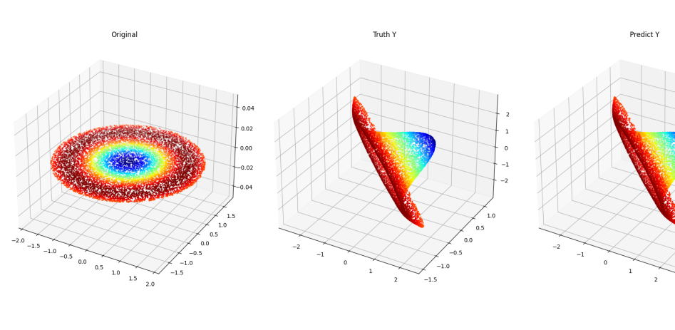
Figure 3. Two-dimensional Rings dataset (left) with a linear representation of the color-coded true responses (right) following a diffeomorphism on the domain with one added dummy dimension.

10. Implementation

The model is implemented in Python using a dynamic programming approach, with objective function

$$\sum\limits_{q=1}^{m}\frac{1}{T_{q}}\sum\limits_{i=0}^{T_{q}-1}\sum\limits_{k,l=1}^{N}a_{k}^{q}(i/T_{q})^{T}K_{q}(z_{k}^{q}(i/T_{q}) ,z_{l}^{q}(i/T_{q}))a_{l}^{q}(i/T_{q})$$

$$+\lambda\sum\limits_{q=0}^{m}U_{q}({A}_{q})+\frac{1}{\sigma^{2}}\sum\limits_{k=1}^{N}\Gamma_{k}(\pi_{r}(\zeta_{k}^{m+1}))$$

minimized over

$$\boldsymbol{a}^{q}(i/T_{q})=(a_{1}^{q}(i/T_{q}),\dots,a_{N}^{q}(i/T_{q}))\in(\mathbb{R}^{d_{q}})^{N},\quad i=0,\dots,T_{q}-1,\quad q=1,\dots,m$$

and ${A}_{0},\dots,{A}_{m},$ i.e.,

$$M_{q}\in\mathcal{M}_{d_{q+1},d_{q}}(\mathbb{R}),\mbox{ }b_{q}\in\mathbb{R}^{d_{q+1}},\quad q=0,\dots,m,$$

subject to

$$z_{k}^{q}((i+1)/T_{q})=z_{k}^{q}(i/T_{q})+\frac{1}{T_{q}}\sum_{l=1}^{N}K_{q}(z_{k}^{q}(i/T_{q}),z_{l}^{q}(i/T_{q}))a_{l}^{q}(i/T_{q})$$

with $z_{k}^{q}(0)=\zeta_{k}^{q}={A}_{q-1}(\xi_{k}^{q-1}),$ $\xi_{k}^{q}=z_{k}^{q}(1),$ and initialization $\xi_{k}^{0}=\iota_{s}(x_{k}).$ The model parameters are initialized as

1. $\boldsymbol{a}^{q}(i/T_{q})=0\in(\mathbb{R}^{d_{q}})^{N},\quad i=0,\dots,T_{q}-1,\quad q=1,\dots,m$

2. $M_{q}\sim\mathcal{N}(0,0.01^{2})\in\mathcal{M}_{d_{q+1},d_{q}}(\mathbb{R}),$ $b_{q}=0\in\mathbb{R}^{d_{q+1}},\quad q=0,\dots,m.$

We include an option to speed up kernel computations using PyKeOps (Charlier et al., 2021) with user-specified precision and GPUs. Our optimization algorithms are gradient descent methods implemented with line search.

To run the model, the user specifies an arbitrary sequence and number of non-identity A and D modules, dimension parameters $s,$ $r,$ and $d_{1},\dots,d_{m},$ ridge regularization weight $\lambda,$ and optimization algorithm parameters for gradient descent, including stopping thresholds and maximum number of iterations. For each D_q module, the user specifies the kernel type and the number of discretized time points $T_{q}$ for state and costate propagation and the control variables. For each kernel $K_{q},$ the algorithm assumes a default kernel width $h_{q}$ of 0.5, as the affine module preceding D_q automatically scales and adapts its input to the kernel width of the subsequent D${}_{q}.$ Input and output dimension assignments for each module in the sequence are automated by our algorithm based on $d_{X},$ $d_{Y},$ $s,$ $r,$ and the inner module dimensions provided by the user. The normalization factor $\sigma$ of the error term is determined by our model as a function of the training data and initial training iterations, as described in Section 12.

11. Data Preprocessing

Prior to training, the $\boldsymbol{x}$ and $\boldsymbol{y}$ training data in $\mathcal{T}_{0}$ are standardized to zero mean and unit variance by subtracting their respective means, ${\mu_{X}\in\mathbb{R}^{d_{X}}}$ and ${\mu_{Y}\in\mathbb{R}^{d_{Y}},}$ and dividing by their respective standard deviations, ${\sigma_{X}\in\mathbb{R}^{d_{X}}}$ and ${\sigma_{Y}\in\mathbb{R}^{d_{Y}}.}$ The test predictors are standardized using the standardization parameters of the training predictors, $\mu_{X}$ and $\sigma_{X}.$ For $s>0,$ $s$ extra dimensions are then appended to the training and test predictors by $N$ vector draws from $\mathcal{N}(0,0.01^{2})\in\mathbb{R}^{s}$ and $N_{\mathit{test}}$ zero vectors $0\in\mathbb{R}^{s},$ respectively, where $N_{\mathit{test}}$ is the number of data points in the test set.

12. Normalization Factor and Model Training

To determine an optimal penalty for endpoint matching errors, the $\sigma$ normalization factor of the error term is calculated by the model as follows. For each data point $x_{i}$ in the unappended, standardized $\mathcal{T}_{0},$ $(y_{j}-y_{i}),j\in J_{i}$ is linearly regressed on ${(x_{j}-x_{i}),j\in J_{i}},$ where $J_{i}$ indexes the $k$ nearest neighbors of $x_{i}$ for ${k=\min\left\{2d_{X}+1,\lfloor\frac{N}{5}\rfloor\right\}.}$ This regression (without intercept) estimates “gradients” $g_{i}\in\mathcal{M}_{d_{Y},d_{X}}(\mathbb{R})$, with residuals

$$r_{ji}=(y_{j}-y_{i})-g_{i}(x_{j}-x_{i}),j\in J_{i}$$

and mean square error

$$\sigma^{2}_{\mathrm{MSE}}=\frac{1}{Nkd_{Y}}\sum_{i=1}^{N}\sum_{j\in J_{i}}\|r_{ji}\|^{2}.$$

The initial $\sigma$ is set to

$$\sigma^{2}=N^{\frac{1}{2}}\max\left\{\sqrt{\sigma^{2}_{\mathrm{MSE}}}/2,0.01\right\},$$

Training begins with the initialized model parameters $\boldsymbol{a}^{1}(\cdot),\dots,\boldsymbol{a}^{m}(\cdot),$ ${A}_{0},\dots,{A}_{m},$ the initial $\sigma,$ and the appended, standardized training data. The model iteratively decreases $\sigma$ until the training MSE

$$\frac{1}{N}\sum_{k=1}^{N}\Gamma_{k}(\sigma_{Y}\odot\pi_{r}(\zeta_{k}^{m+1})+\mu_{Y}),$$

using the unstandardized experimental responses $y_{k},$ is less than

$$\max\left\{\sigma^{2}_{\mathrm{MSE}},0.01\right\}$$

or a maximum number of model loops are reached. Using the final value for $\sigma$ and parameters $\boldsymbol{a}^{1}(\cdot),\dots,\boldsymbol{a}^{m}(\cdot),{A}_{0},\dots,{A}_{m}$ initialized to their final values in this step, a final training loop through the model is executed to complete training.

13. Evaluation Metric

The diffeomorphisms and affine transformations learned on the training set are applied to the corresponding test set for performance analysis. Specifically, the test predictors are forward propagated through the model, transformed in turn by the learned affine transformations of each A_q and the vector fields of each D${}_{q},$ the latter functions of the learned $\boldsymbol{a}^{q}(\cdot)$ and cached $\boldsymbol{z}^{q}(\cdot).$ The evaluation metric is root-MSE (RMSE) between the model outputs $\zeta_{k,\mathit{test}}^{m+1}$ and the test experimental responses

$$\sqrt{\frac{1}{N_{\mathit{test}}}\sum_{k=1}^{N_{\mathit{test}}}\Gamma_{k}(\sigma_{Y}\odot\pi_{r}(\zeta_{k,\mathit{test}}^{m+1})+\mu_{Y})},$$

which we will denote test RMSE.

14. Baseline Experiments

While DA and AD are the smallest possible sequences that can be represented in our model, the AD sequence is not as practical for regression purposes, and the DA sequence requires the user to specify a data-specific kernel width for the D₁ diffeomorphism. Therefore, we consider the ADA model, which is the sequence case for $m=1$ and no identity modules, as our simplest regression model sequence, and we choose this baseline model for our experiments, as shown in Figure 4. Additionally, we choose the simplest reasonable values for our model parameters. We set $\lambda=1$ and assign dimensions ${s=1,}$ ${r=0,}$ and ${d_{1}=d_{X}+s,}$ ensuring the dummy dimension added to the dataset is carried through module A₀ to the diffeomorphism in D${}_{1}.$ For module D${}_{1},$ we set ${T_{1}=10}$, and we construct a matrix-valued kernel from the scalar Matérn kernel and the identity matrix $\mathrm{I}_{d_{1}}$ (Younes, 2020). In particular,

$$K_{1}(x,y)=\left(1+u+0.4u^{2}+\frac{1}{15}u^{3}\right)e^{-u}\mathrm{I}_{d_{1}},\quad u=\frac{|y-x|}{h_{1}}$$

with default kernel width $h_{1}=0.5$. The optimization algorithm is the limited-memory Broyden–Fletcher–Goldfarb–Shanno algorithm (L-BFGS) with Wolfe conditions on the line search. Early stopping, typically used to prevent overfitting, is avoided by setting the maximum number of gradient descent iterations large enough to ensure numerical convergence.

Figure 4. ADA transformation sequence used in the experiments.

Our model is tested on nine UCI datasets—Concrete, Energy, Kin8nm, Naval, Power, Protein, Wine Red, Yacht, and Year—with standard splits originally generated for the experiments in Hernandez-Lobato and Adams (2015) and gap splits generated by Foong et al. (2019). Datasets are split into training and test sets by uniform subsampling for the standard splits and by a custom split assigning “outer regions” to the training sets and “middle regions” to the test sets for the gap splits. For the standard splits, 20 randomized train-test splits (90% train, 10% test) of each dataset are provided, with the exception of the larger Protein (5 splits) and Year (1 split) datasets. Note that the Year standard split is not provided in the standard splits repositories, so we assume it follows the single split (90% train, 10% test) guideline provided for that dataset in the UCI respository. For the gap splits, $d_{X}$ train-test splits of each dataset are provided, each split corresponding to one of the $d_{X}$ dimensions of that dataset. These splits are generated by sorting the data points in increasing order in the dimension of interest, then assigning the middle third to the test set and the outer two-thirds to the training set. The Year dataset is not included in the gap splits repository or experiments. For each multiple split experiment, the evaluation metric is test RMSE averaged over all splits with standard error.

The total number of data points $N_{T}$ prior to splitting and the dimensions $d_{X}$ and $d_{Y}$ of each provided dataset are listed in Tables 3A and 3B. Note that although two of the original datasets—Energy and Naval—have response dimension ${d_{Y}=2,}$ all provided standard and gap splits have $d_{Y}=1.$ In the Year dataset (${N_{T}=515345,}$ ${d_{X}=90}$) experiment, to make it computationally tractable, we set $d_{1}=10$ to reduce dimensionality and train the diffeomorphisms on a training data subset ($N_{S}=1000$) selected from the training data as the initial $N_{S}$ cluster seeds for $k$-means clustering according to the $k$-means++ algorithm. Kernel computations are performed using PyKeOps in all experiments.

We implement standard ridge regression (A) and five DNNs for performance comparison with our model. Ridge regression is implemented in Python with regularization weight ${\lambda=1.}$ The DNN models, implemented in TensorFlow and denoted DNN-x, ${\mathrm{x}=1,2,3,5,10}$, consist of x sequential densely-connected hidden layers with ReLU activation and layer sizes listed in Table 1, followed by a densely-connected output layer. In TensorFlow, we use the Adam optimizer (Kingma and Ba, 2015), MSE loss, and 400 training epochs or number of complete passes through the training datasets. Default values are assumed for all other TensorFlow parameters, including learning rate of 0.001, batch size of 32, and no validation split of the data. The A and DNN models are trained and tested on the standardized datasets, and the standardization is removed from the model outputs for performance analysis.

Table 1. Hidden Layer Sizes of Densely-Connected Neural Networks.

Hidden Layer Model 1 2 3 4 5 6 7 8 9 10 DNN-1 64 DNN-2 128 64 DNN-3 256 128 64 DNN-5 256 128 64 32 16 DNN-10 256 128 64 32 16 16 8 8 4 4

Performance of our ADA model is compared in Tables 3A and 3B with the A and DNN models and with RMSE experimental results found in the literature using the same standard splits and gap splits. The literature results in those tables are the top performing models from each literature reference in Table 2 that conducted experiments on the same standard splits and gap splits. A comprehensive list of all Table 2 results is found in Appendix Tables C.1A and C.1B for standard split experiments and Tables C.2A and C.2B for gap split experiments. Gray shading in Tables C.1A and C.1B indicates experiments using standard splits that are different from those used in our experiments but generated following the training-test protocol from Hernandez-Lobato and Adams (2015). The literature models include Bayesian deep learning techniques such as variational inference (VI); backpropagation (BP) and probabilistic BP (PBP) for Bayesian NNs (BNNs); Monte Carlo dropout run in a timed setting (Dropout-TS or Dropout), to convergence (Dropout-C), and with grid hyperparameter tuning (Dropout-G); BNNs with variational matrix Gaussian posteriors (VMG) and horseshoe priors (HS-BNN); and PBP with the matrix variate Gaussian distribution (PBP-MV). Additional models are Bayes by backprop (BBB); stochastic, low-rank, approximate natural-gradient (SLANG) method; variations of the neural linear (NL) model: maximum a posteriori (MAP) estimation NL (MAP NL), regularized NL (Reg NL), Bayesian noise (BN) NL by marginal likelihood maximization (BN(ML) NL) and by Bayesian optimization (BO) (BN(BO) NL); depth uncertainty network (DUN) with multi-layer perceptron (MLP) architecture (DUN (MLP)); deep ensembles (Ensemble); Gaussian mean field VI (MFVI); vanilla NNs (SGD); and distributional regression by negative log-likelihood (NLL) with alternative loss formulation ($\beta\mathrm{-NLL}$) ($\mathcal{L}_{\beta\mathrm{-NLL}}$), “moment matching” (MM) ($\mathcal{L}_{\mathrm{MM}}$), MSE loss ($\mathcal{L}_{\mathrm{MSE}}$), Student’s t-distribution (Student-t), and different variance priors and variational inference (xVAMP, xVAMP*, VBEM, VBEM*). An integer “-x” appended to a model name denotes x hidden layers in the network. All presented literature results involve some form of hyperparameter tuning, typically by BO or a grid approach, using a portion of each training set as a validation set.

Table 2. Literature Models Tested on Standard Splits (S), Gap Splits (G), and Different Standard Splits (D).

Models Splits Reference VI, BP, PBP S Hernandez-Lobato and Adams (2015) Dropout-TS S Gal and Ghahramani (2016) VMG D Louizos and Welling (2016) HS-BNN D Ghosh et al. (2019) PBP-MV D Sun et al. (2017) Dropout-C, Dropout-G S Mukhoti et al. (2018) BBB, SLANG S Mishkin et al. (2018) MAP, MAP NL, Reg NL, D,G Ober and Rasmussen (2019) BN(ML) NL, BN(BO) NL DUN, DUN (MLP), Dropout, S,G Antoran et al. (2020) Ensemble, MFVI, SGD $\mathcal{L}_{\beta\mathrm{-NLL}},$ $\mathcal{L}_{\mathrm{MM}},$ $\mathcal{L}_{\mathrm{MSE}},$ Student-t, S,D Seitzer et al. (2022) xVAMP, xVAMP*, VBEM, VBEM*

For consistency in performance comparison, we convert the standard deviation results in Ghosh et al. (2019), Antoran et al. (2020), and Seitzer et al. (2022) to standard errors and use the standard error representation of the results in Gal and Ghahramani (2016) found in Mukhoti et al. (2018). Due to size, the larger Protein and Year datasets are not analyzed in some of the literature references. Louizos and Welling (2016) and Sun et al. (2017) generate their own standard splits, following the training-test protocol from Hernandez-Lobato and Adams (2015), and randomly generate the Year data split. Seitzer et al. (2022) also generate their own standard splits for the Energy and Naval datasets (maintaining the original response dimensions of $d_{Y}=2$) and use the standard splits from Hernandez-Lobato and Adams (2015) for the rest of the datasets. In Ghosh et al. (2019) and Ober and Rasmussen (2019), it is unclear if the standard splits are those used in Hernandez-Lobato and Adams (2015) or if they are generated by the authors following that training-test protocol, thus these results are shaded in gray in Tables C.1A and C.1B. All literature results are provided in 2-digit decimal precision, with the exception of 3-digit decimal precision in Hernandez-Lobato and Adams (2015), Antoran et al. (2020) and the Kin8nm and Wine Red analysis in Seitzer et al. (2022) and 4-digit decimal precision for the Naval analysis in Seitzer et al. (2022).

The lowest average test RMSE in each standard splits column and each gap splits column in Tables 3A and 3B is bolded, determined in the Kin8nm and Naval standard split columns and the Kin8nm and Wine Red gap split columns by a comparison of results in higher decimal precision. Result values in these four columns from sources with only 2-digit decimal representation that cannot be confirmed as lower or higher than these lowest values are bolded as well. Examples of final reshaped sequences through module D₁ of standard training splits of Kin8nm, Concrete, and Energy are illustrated in Figures 5, 6, and 7, respectively. In each figure plot, data point locations represent the first three principal components of $\boldsymbol{z}^{1}(t)$ at a fixed time $t,$ and color coding represents the true responses. Each figure contains six plots, corresponding to $t=0,$ 0.2, 0.4, 0.6, 0.8, and 1, respectively.

Table 3A. Average test RMSE $\pm$ 1 standard error (best values in bold).

UCI Standard Splits (Top) and Gap Splits (Bottom) Concrete Energy Kin8nm Naval Power $N_{T}=1030$ $N_{T}=768$ $N_{T}=8192$ $N_{T}=11934$ $N_{T}=9568$ $d_{X}=8$ $d_{X}=8$ $d_{X}=8$ $d_{X}=16$ $d_{X}=4$ Model $d_{Y}=1$ $d_{Y}=1$ $d_{Y}=1$ $d_{Y}=1$ $d_{Y}=1$ ADA $4.93\pm 0.13$ $0.50\pm 0.01$ $\mathbf{0.07\pm 0.00}$ ¹ $\mathbf{0.00\pm 0.00}$ ¹ $\mathbf{3.36\pm 0.05}$ A $10.31\pm 0.14$ $3.06\pm 0.05$ $0.20\pm 0.00$ $0.01\pm 0.00$ $4.61\pm 0.03$ DNN-1 $5.02\pm 0.14$ $0.53\pm 0.01$ $0.08\pm 0.00$ $0.00\pm 0.00$ $3.98\pm 0.04$ DNN-2 $4.47\pm 0.13$ $0.51\pm 0.01$ $0.08\pm 0.00$ $0.00\pm 0.00$ $3.70\pm 0.04$ DNN-3 $\mathbf{4.46\pm 0.12}$ $\mathbf{0.43\pm 0.02}$ $0.08\pm 0.00$ $0.00\pm 0.00$ $3.63\pm 0.05$ DNN-5 $4.71\pm 0.15$ $0.46\pm 0.02$ $0.08\pm 0.00$ $0.00\pm 0.00$ $3.67\pm 0.05$ DNN-10 $4.64\pm 0.14$ $0.54\pm 0.08$ $0.08\pm 0.00$ $0.01\pm 0.00$ $3.59\pm 0.04$ BP-3 $5.57\pm 0.13$ $0.63\pm 0.03$ $0.07\pm 0.00$ $0.00\pm 0.00$ $4.11\pm 0.04$ BP-4 $5.53\pm 0.14$ $0.67\pm 0.03$ $0.07\pm 0.00$ $0.00\pm 0.00$ $4.18\pm 0.06$ PBP-2 $5.24\pm 0.12$ $0.90\pm 0.05$ $0.07\pm 0.00$ $0.00\pm 0.00$ $4.03\pm 0.03$ PBP-3 $5.73\pm 0.11$ $1.24\pm 0.06$ $0.07\pm 0.00$ $0.01\pm 0.00$ $4.07\pm 0.04$ Dropout-TS $5.23\pm 0.12$ $1.66\pm 0.04$ $0.10\pm 0.00$ $0.01\pm 0.00$ $4.02\pm 0.04$ Dropout-C $4.93\pm 0.14$ $1.08\pm 0.03$ $0.09\pm 0.00$ $\mathbf{0.00\pm 0.00}$ $4.00\pm 0.04$ Dropout-G $4.82\pm 0.16$ $0.54\pm 0.06$ $0.08\pm 0.00$ $\mathbf{0.00\pm 0.00}$ $4.01\pm 0.04$ BBB $6.16\pm 0.13$ $0.97\pm 0.09$ $0.08\pm 0.00$ $\mathbf{0.00\pm 0.00}$ $4.21\pm 0.03$ SLANG $5.58\pm 0.19$ $0.64\pm 0.03$ $0.08\pm 0.00$ $\mathbf{0.00\pm 0.00}$ $4.16\pm 0.04$ DUN (MLP) $4.57\pm 0.16$ $0.95\pm 0.11$ $0.08\pm 0.00$ ${0.00\pm 0.00}$ $3.67\pm 0.06$ Dropout $4.61\pm 0.13$ $0.57\pm 0.05$ $0.07\pm 0.00$ ${0.00\pm 0.00}$ $3.82\pm 0.08$ Ensemble $4.55\pm 0.13$ $0.51\pm 0.02$ $0.30\pm 0.22$ ${0.00\pm 0.00}$ $3.44\pm 0.05$ $\mathbf{\mathcal{L}_{\beta-NLL}(\beta=0.75)}$ $5.67\pm 0.16$ $--$ $0.08\pm 0.00$ $--$ $4.04\pm 0.03$ $\mathbf{\mathcal{L}_{MSE}}$ $4.96\pm 0.14$ $--$ $0.08\pm 0.00$ $--$ $4.01\pm 0.04$ VBEM* $5.17\pm 0.13$ $--$ $0.08\pm 0.00$ $--$ $4.02\pm 0.04$ ADA $7.53\pm 0.29$ $3.61\pm 1.23$ $\mathbf{0.07\pm 0.00}$ ¹ $0.02\pm 0.00$ $5.53\pm 0.58$ A $10.75\pm 0.29$ $3.96\pm 0.36$ $0.20\pm 0.00$ $0.03\pm 0.00$ $4.47\pm 0.08$ DNN-1 $7.53\pm 0.34$ $4.59\pm 1.75$ $0.08\pm 0.00$ $0.03\pm 0.00$ $4.33\pm 0.13$ DNN-2 $7.45\pm 0.31$ $3.77\pm 1.34$ $0.08\pm 0.00$ $0.03\pm 0.00$ $5.17\pm 0.33$ DNN-3 $7.44\pm 0.23$ $3.93\pm 1.42$ $0.08\pm 0.00$ $0.03\pm 0.00$ $5.67\pm 0.33$ DNN-5 $7.28\pm 0.16$ $3.23\pm 1.08$ $0.08\pm 0.00$ $0.03\pm 0.00$ $5.78\pm 0.41$ DNN-10 $8.41\pm 1.05$ $5.98\pm 1.42$ $0.08\pm 0.00$ $0.02\pm 0.00$ $5.56\pm 0.45$ MAP-1 $7.79\pm 0.18$ $\mathbf{2.83\pm 0.99}$ $0.09\pm 0.01$ $0.02\pm 0.00$ $\mathbf{4.24\pm 0.12}$ MAP-2 $7.78\pm 0.23$ $3.70\pm 1.33$ $0.08\pm 0.00$ $0.03\pm 0.00$ $4.33\pm 0.18$ MAP-2 NL $7.44\pm 0.17$ $3.48\pm 1.21$ $\mathbf{0.07\pm 0.00}$ $0.03\pm 0.00$ $4.27\pm 0.08$ BN(ML)-2 NL $7.33\pm 0.36$ $4.10\pm 1.64$ $0.08\pm 0.00$ $\mathbf{0.01\pm 0.00}$ $5.17\pm 0.28$ DUN $7.20\pm 0.18$ $2.94\pm 0.67$ $0.08\pm 0.00$ $0.02\pm 0.00$ $4.30\pm 0.09$ Dropout $7.06\pm 0.21$ $2.87\pm 0.50$ $0.07\pm 0.00$ $0.03\pm 0.00$ $4.69\pm 0.07$ Ensemble $\mathbf{6.85\pm 0.18}$ $3.36\pm 0.83$ $1.63\pm 0.99$ $0.02\pm 0.00$ $4.37\pm 0.09$ MFVI $7.55\pm 0.19$ $8.61\pm 2.10$ $0.10\pm 0.01$ $0.03\pm 0.01$ $4.68\pm 0.16$

• Lowest results in their respective column sections, when compared in higher decimal precision.
  Also bolded are 2-digit decimal literature results that cannot be confirmed as lower or higher
  than these lowest results.

Table 3B. Average test RMSE $\pm$ 1 standard error (best values in bold).

UCI Standard Splits (Top) and Gap Splits (Bottom) Protein Wine Red Yacht Year $N_{T}=45730$ $N_{T}=1599$ $N_{T}=308$ $N_{T}=515345$ $d_{X}=9$ $d_{X}=11$ $d_{X}=6$ $d_{X}=90$ Model $d_{Y}=1$ $d_{Y}=1$ $d_{Y}=1$ $d_{Y}=1$ ADA $3.33\pm 0.05$ $\mathbf{0.59\pm 0.01}$ $0.72\pm 0.06$ $\mathbf{8.84\pm\mbox{NA}}$ A $5.21\pm 0.02$ $0.65\pm 0.01$ $8.95\pm 0.27$ $9.51\pm\mbox{NA}$ DNN-1 $4.35\pm 0.04$ $0.66\pm 0.01$ $0.95\pm 0.07$ $8.96\pm\mbox{NA}$ DNN-2 $3.79\pm 0.02$ $0.73\pm 0.02$ $0.92\pm 0.08$ $9.78\pm\mbox{NA}$ DNN-3 $3.83\pm 0.03$ $0.66\pm 0.02$ $1.27\pm 0.15$ $10.73\pm\mbox{NA}$ DNN-5 $3.70\pm 0.01$ $0.64\pm 0.01$ $1.22\pm 0.12$ $10.20\pm\mbox{NA}$ DNN-10 $4.73\pm 0.52$ $0.70\pm 0.02$ $3.32\pm 1.02$ $10.31\pm\mbox{NA}$ BP-3 $4.01\pm 0.03$ $0.65\pm 0.01$ $1.11\pm 0.09$ $8.93\pm\mbox{NA}$ BP-4 $3.96\pm 0.01$ $0.65\pm 0.02$ $1.27\pm 0.13$ $9.05\pm\mbox{NA}$ PBP-2 $4.25\pm 0.02$ $0.64\pm 0.01$ $0.85\pm 0.05$ $8.92\pm\mbox{NA}$ PBP-3 $4.09\pm 0.03$ $0.64\pm 0.01$ $0.89\pm 0.10$ $8.87\pm\mbox{NA}$ Dropout-TS $4.36\pm 0.01$ $0.62\pm 0.01$ $1.11\pm 0.09$ $8.85\pm\mbox{NA}$ Dropout-C $4.27\pm 0.01$ $0.61\pm 0.01$ $0.70\pm 0.05$ $--$ Dropout-G $4.27\pm 0.02$ $0.62\pm 0.01$ $0.67\pm 0.05$ $--$ BBB $--$ $0.64\pm 0.01$ $1.13\pm 0.06$ $--$ SLANG $--$ $0.65\pm 0.01$ $1.08\pm 0.06$ $--$ DUN (MLP) $3.41\pm 0.03$ $0.63\pm 0.01$ $2.47\pm 0.19$ $--$ Dropout $3.43\pm 0.03$ $0.64\pm 0.01$ $0.88\pm 0.09$ $--$ Ensemble $\mathbf{3.26\pm 0.03}$ $1.93\pm 1.28$ $1.43\pm 0.11$ $--$ $\mathbf{\mathcal{L}_{\beta-NLL}(\beta=0.75)}$ $4.28\pm 0.01$ $0.64\pm 0.01$ $1.97\pm 0.23$ $--$ $\mathbf{\mathcal{L}_{MSE}}$ $4.28\pm 0.03$ $0.63\pm 0.01$ $0.78\pm 0.06$ $--$ VBEM* $4.35\pm 0.04$ $0.63\pm 0.01$ $\mathbf{0.65\pm 0.04}$ $--$ ADA $5.10\pm 0.18$ $0.68\pm 0.01$ $1.03\pm 0.14$ A $5.34\pm 0.04$ $0.64\pm 0.01$ $9.24\pm 0.31$ DNN-1 $5.08\pm 0.09$ $0.72\pm 0.01$ $2.33\pm 0.29$ DNN-2 $5.56\pm 0.20$ $0.81\pm 0.01$ $3.40\pm 0.64$ DNN-3 $5.95\pm 0.21$ $0.73\pm 0.01$ $3.53\pm 0.59$ DNN-5 $5.85\pm 0.24$ $0.74\pm 0.01$ $3.29\pm 0.54$ DNN-10 $6.04\pm 0.21$ $0.76\pm 0.01$ $3.95\pm 0.71$ MAP-1 $5.16\pm 0.04$ $\mathbf{0.63\pm 0.01}$ $1.31\pm 0.14$ MAP-2 $5.07\pm 0.06$ $\mathbf{0.63\pm 0.01}$ $1.05\pm 0.09$ MAP-2 NL $5.08\pm 0.06$ $\mathbf{0.63\pm 0.01}$ $\mathbf{1.01\pm 0.09}$ BN(ML)-2 NL $5.37\pm 0.17$ $0.64\pm 0.01$ $1.31\pm 0.16$ DUN $5.21\pm 0.35$ $0.70\pm 0.01$ $1.85\pm 0.17$ Dropout $5.13\pm 0.28$ $0.66\pm 0.01$ $2.29\pm 0.47$ Ensemble $\mathbf{4.80\pm 0.27}$ $0.67\pm 0.01$ $1.84\pm 0.19$ MFVI $5.12\pm 0.13$ $\mathbf{0.63\pm 0.01}$ ¹ $1.84\pm 0.16$

• Lowest results in their respective column sections, when compared in higher
  decimal precision. Also bolded are 2-digit decimal literature results that cannot
  be confirmed as lower or higher than these lowest results.

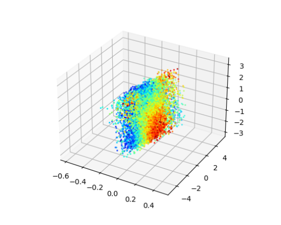
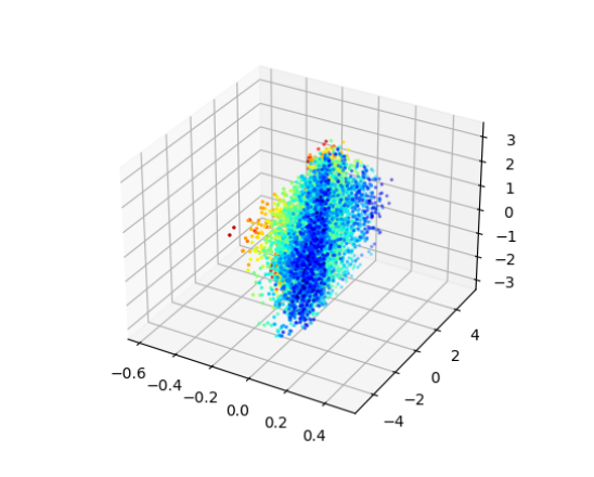
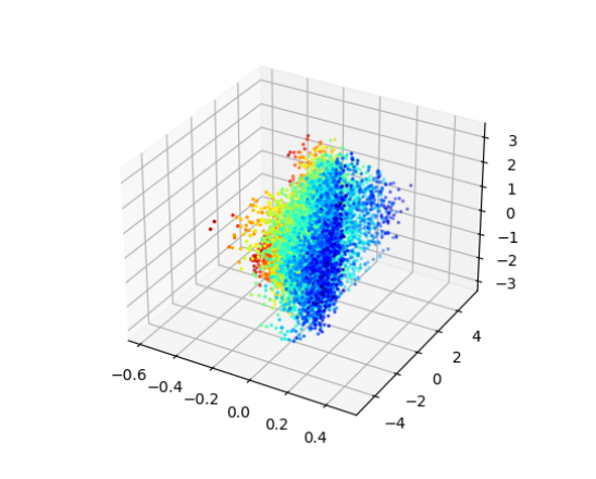
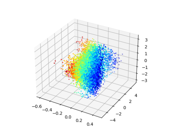
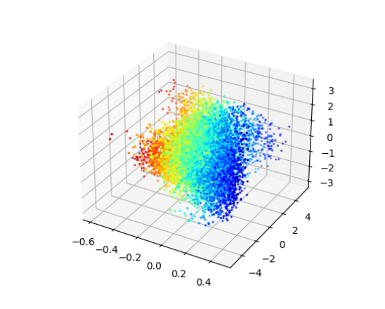
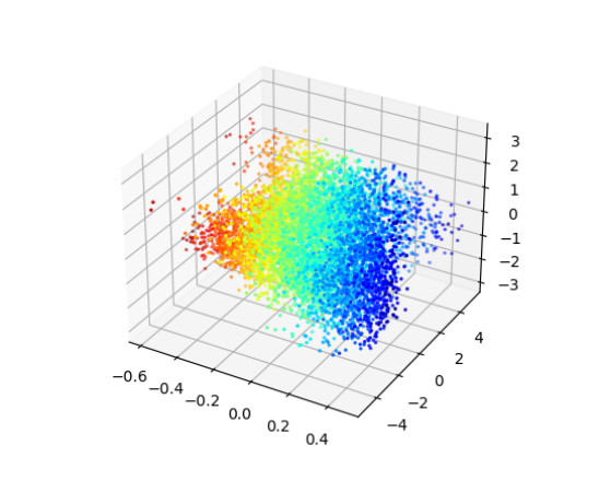
Figure 5. Reshaped sequence of a Kin8nm standard training split through module D${}_{1}.$ Each plot corresponds to the first three principal components of $\boldsymbol{z}^{1}(t)$ at a fixed time $t,$ with the true responses color coded. Starting at top and viewing left to right, $t=0,$ 0.2, 0.4, 0.6, 0.8, and 1, respectively.

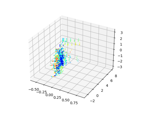
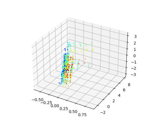
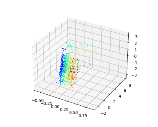
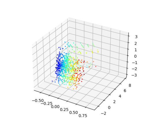
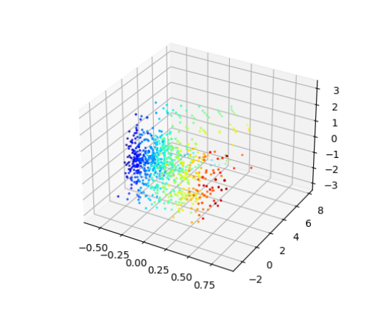
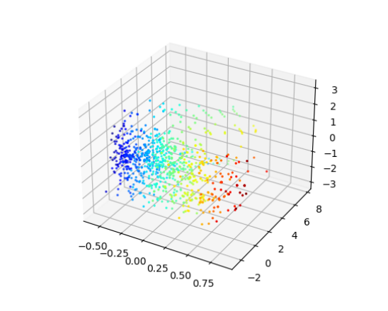
Figure 6. Reshaped sequence of a Concrete standard training split through module D${}_{1}.$ Each plot corresponds to the first three principal components of $\boldsymbol{z}^{1}(t)$ at a fixed time $t,$ with the true responses color coded. Starting at top and viewing left to right, $t=0,$ 0.2, 0.4, 0.6, 0.8, and 1, respectively.

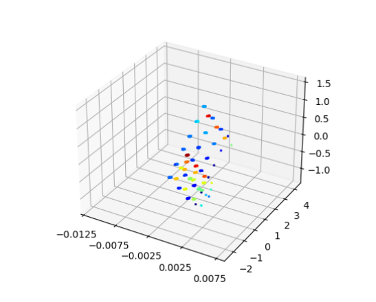
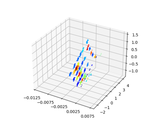
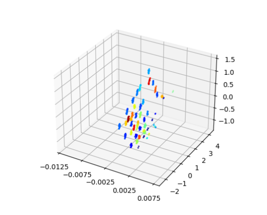
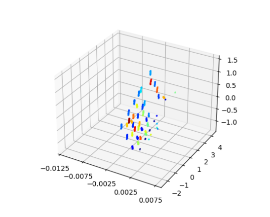
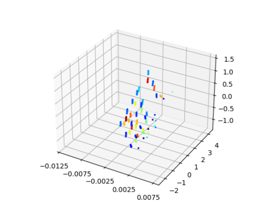
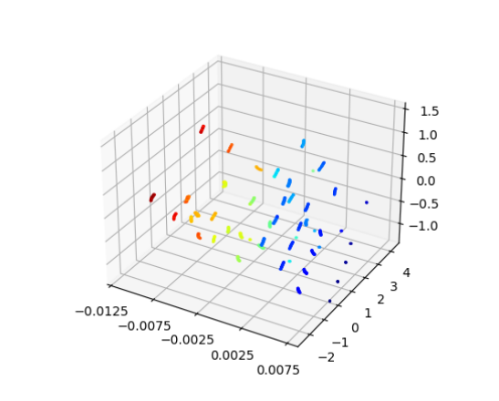
Figure 7. Reshaped sequence of an Energy standard training split through module D${}_{1}.$ Each plot corresponds to the first three principal components of $\boldsymbol{z}^{1}(t)$ at a fixed time $t,$ with the true responses color coded. Starting at top and viewing left to right, $t=0,$ 0.2, 0.4, 0.6, 0.8, and 1, respectively.

15. Discussion

In comparison with all models tested on the same UCI standard splits in Tables 3A and 3B, our baseline ADA model performs well in general, ranking lowest in average test RMSE for five datasets (Kin8nm, Naval , Power, Wine Red, and Year), second lowest for Protein, third lowest for Energy, and fourth lowest for Yacht. Additionally, the use of subset training and dimensionality reduction for the Year experiment ensures experiment tractability and significantly reduces its running time. The DNN-3 model outperforms all models for the Concrete and Energy datasets, and Ensemble and VBEM* have the lowest average RMSEs for Protein and Yacht, respectively. In comparison with all models tested on different standard splits in Tables C.1A and C.1B, our ADA model maintains a similar performance level, as those literature model experiments—with the exception of the Year dataset on which PBP-MV performs best—primarily show improved performance for the smaller Energy and Yacht datasets on which ADA did not have top performance. Sample D₁ deformation sequences in Figures 5-7 from these experiments demonstrate the smooth invertibility of data transformations through the D modules of our model.

While the standard splits are useful for testing a model’s ability to fit data, the gap splits can test in a sense how well a model generalizes to out-of-distribution data. A robust model will simultaneously perform well on the standard splits and not critically fail on the gap splits. Our ADA model demonstrates above average performance overall in ranking comparisons with all models tested on the UCI gap splits in Tables 3A and 3B, with no excessively poor predictions. Specifically, our model’s average test RMSE ranks lowest for Kin8nm, second lowest for Yacht, fifth lowest for Protein, twelfth lowest (fourth highest) for Power, and approximately center ranking performance for Concrete, Energy, Naval, and Wine Red.

16. Beyond the Baseline

We test more complex model architectures beyond the ADA baseline in Table 4, using the Airfoil dataset in the UCI repository for the experiments. Performance is compared with DNNs, as the Airfoil dataset has similar size and dimensions to the Concrete and Energy datasets on which the DNN models perform best in Table 3A. We generate 10 randomized train-test splits (90% train, 10% test) and again evaluate prediction performance of the test splits. The parameters of the diffeomorphic regression models in Table 4 follow those in the experiments in Section 14, including the same A and D modules used in our ADA model, with two exceptions. First, for (AD)^xA models with x sequential AD module pairs, the affine costs of the inner A modules are the functions

$$U_{q}({A})=\left\|M-\mathrm{I}_{d}\right\|^{2}=\mathrm{trace}((M-\mathrm{I}_{d})^{T}(M-\mathrm{I}_{d})),\quad q=1,\dots,m-1$$

for affine transformations from $\mathbb{R}^{{d_{q}}}$ to $\mathbb{R}^{{d_{q}}}$ (here, $d_{q+1}=d_{q}$) of the form ${A}(x)=Mx+b,$ ${M\in\mathcal{M}_{d_{q}}(\mathbb{R}),}$ ${b\in\mathbb{R}^{d_{q}}.}$ The initialization of these inner A modules is

$$M_{q}=\mathrm{I}_{d_{q}}+\mathrm{diag}(w),w\sim\mathcal{N}(0,0.01^{2})\in\mathbb{R}^{d_{q}},\hskip 2.84544ptb_{q}=0\in\mathbb{R}^{d_{q}},\quad q=1,\dots,m-1.$$

Second, for AD^xA models with x sequential D modules, while the D modules have the same dimension, kernel type, and number of discretized time points as in our ADA model, the kernel widths of this sequence of $m$ D modules increase ($h_{q}\uparrow$), with respective values $\frac{1}{m+1},\frac{2}{m+1},\dots,\frac{m}{m+1}$, or decrease ($h_{q}\downarrow$), with respective values $\frac{m}{m+1},\frac{m-1}{m+1},\dots,\frac{1}{m+1}.$ All other experimental parameters in Table 4 are the same as in Section 14. Starting with the original ADA model, the results show improved performance with increased model complexity, with the AD⁴A ($h_{q}\downarrow$) model outperforming all models, including the DNNs. Note that to ensure these improved results are not the result of the increased number of time steps inherent in increasing the number of D modules, the ADA model is also run with increased $T_{1}$, as shown in Table 4.

Table 4. Average test RMSE $\pm$ 1 standard error (best values in bold).

Airfoil $N_{T}=1503$ $d_{X}=5$ Model $d_{Y}=1$ ADA $1.53\pm 0.05$ ADA ($T_{1}=20)$ $1.40\pm 0.06$ ADA ($T_{1}=30)$ $1.43\pm 0.06$ ADA ($T_{1}=40)$ $1.44\pm 0.05$ AD²A ($h_{q}\uparrow$) $1.38\pm 0.05$ AD³A ($h_{q}\uparrow$) $1.33\pm 0.05$ AD⁴A ($h_{q}\uparrow$) $1.32\pm 0.05$ AD²A ($h_{q}\downarrow$) $1.25\pm 0.04$ AD³A ($h_{q}\downarrow$) $1.18\pm 0.03$ AD⁴A ($h_{q}\downarrow$) $\mathbf{1.08\pm 0.03}$ (AD)²A $1.41\pm 0.05$ (AD)³A $1.28\pm 0.04$ (AD)⁴A $1.21\pm 0.05$ (AD)⁵A $1.25\pm 0.05$ DNN-1 $2.02\pm 0.06$ DNN-2 $1.36\pm 0.05$ DNN-3 $1.25\pm 0.05$ DNN-5 $1.16\pm 0.04$ DNN-10 $1.79\pm 0.60$

We test the AD⁴A ($h_{q}\downarrow$) model further in Table 5 on the standard and gap splits of six of the UCI datasets, using the same Section 14 experimental parameters. In comparison with the ADA results, the AD⁴A ($h_{q}\downarrow$) model shows improved (Concrete, Kin8nm, Power) and similar (Energy, Wine Red) results for the standard split experiments, and improved (Concrete, Power) and similar (Kin8nm, Yacht) results for the gap split experiments, with slightly worse performance on average on the remaining experiments—Yacht standard splits and Energy and Wine Red gap splits. In particular, for the standard splits, the improved Concrete result is now comparable with the lowest result in DNN-3, and the improved Kin8nm result is the lowest in both Tables 3A and C.1A. For the gap splits, the improved Concrete result does not improve its ranking in Table 3A but the improved Power result does, bringing its performance up to approximately center ranking.

Table 5. Average test RMSE $\pm$ 1 standard error (best values in bold).

UCI Standard Splits (Top) and Gap Splits (Bottom) Model Concrete Energy Kin8nm Power Wine Red Yacht ADA $4.93\pm 0.13$ $\mathbf{0.50\pm 0.01}$ $0.07\pm 0.00$ $3.36\pm 0.05$ $\mathbf{0.59\pm 0.01}$ $\mathbf{0.72\pm 0.06}$ AD⁴A ($h_{q}\downarrow$) $\mathbf{4.49\pm 0.12}$ $\mathbf{0.50\pm 0.01}$ $\mathbf{0.06\pm 0.00}$ $\mathbf{3.24\pm 0.05}$ $\mathbf{0.59\pm 0.01}$ $0.78\pm 0.05$ ADA $7.53\pm 0.29$ $\mathbf{3.61\pm 1.23}$ $\mathbf{0.07\pm 0.00}$ $5.53\pm 0.58$ $\mathbf{0.68\pm 0.01}$ $\mathbf{1.03\pm 0.14}$ AD⁴A ($h_{q}\downarrow$) $\mathbf{7.47\pm 0.29}$ $3.66\pm 1.15$ $\mathbf{0.07\pm 0.00}$ $\mathbf{4.60\pm 0.23}$ $0.69\pm 0.01$ $\mathbf{1.03\pm 0.18}$

17. Summary

We present a layered approach to multivariate regression using FineMorphs, a sequence model of affine and diffeomorphic transformations. Optimal control concepts from shape analysis are leveraged to optimally “reshape” model states while learning. Diffeomorphisms (the model states) are generated by RKHS time-dependent vector fields (the control) calculated by Hamiltonian control theory, minimizing—along with the optimal affine parameters—a learning objective functional consisting of a kinetic energy term and affine and endpoint costs. In our setting, any arbitrary number and order of arbitrary affine and diffeomorphic transformations is possible, and diffeomorphisms can be generated as flows of sub-optimal vector fields to reduce dataset size and model complexity, while affine modules can scale data prior to diffeomorphic transforms as well as reduce (or increase) dimensionality. For both the optimal and sub-optimal vector fields cases, a proof of the existence of a solution to the variational problem and a derivation of the necessary conditions for optimality are provided. On standard UCI benchmark experiments, our baseline diffeomorphic regression model—ADA—performs favorably overall against state-of-the-art, hyperparameter-tuned deep BNNs and other models in the literature as well as DNNs in TensorFlow. The computational intractability of the largest dataset in the experiments is successfully addressed with our model’s dimensionality and dataset reduction capabilities, with good performance. A general trend of improved performance with increased model complexity is observed, in particular with “coarse-to-fine” models containing multiple sequential diffeomorphisms of decreasing kernel sizes. Additionally, our models demonstrate out-of-distribution robustness with reasonable performances in experiments using custom gap splits, in which the “middle regions” of the data are assigned to the test sets. In general, our diffeomorphic regression models provide an important degree of explainability and interpretability, even for the more complex architectures, as each diffeomorphic module in the model is a smooth invertible transformation of the data. Future work includes further understanding of the theoretical basis, limitations, and advantages of our models; investigating dimensionality reduction and transformer architectures; and improving model run-time through adaptation of L-BFGS or stochastic optimization approaches.

Appendix A Existence of Solution to the FineMorph Variational Problem

The variational problem in (LABEL:eq:obj2) is to minimize

(A.1) $$\begin{split}G(v_{1},\dots,v_{m},M_{0},\dots,M_{m},b_{0},\dots,b_{m})=&\sum_{q=1}^{m}\|v_{q}\|_{\mathcal{H}_{q}}^{2}+\lambda\sum_{q=0}^{m}\|M_{q}\|^{2}\\ &+\frac{1}{\sigma^{2}}\sum_{k=1}^{N}\Gamma_{k}(\pi_{r}(\zeta_{k}^{m+1}))\end{split}$$

over $v_{q}\in\mathcal{H}_{q},$ $q=1,\dots,m,$ and ${M_{q}\in\mathcal{M}_{d_{q+1},d_{q}}(\mathbb{R}),}$ ${b_{q}\in\mathbb{R}^{d_{q+1}}},$ $q=0,\dots,m,$ subject to

(A.2) $$\left\{\begin{aligned} \partial_{t}{\boldsymbol{\varphi}}_{v_{q}}(t)&=v_{q}(t)\circ{\boldsymbol{\varphi}}_{v_{q}}(t),\quad t\in[0,1]\\ \zeta_{k}^{q+1}&=M_{q}{\boldsymbol{\varphi}}_{v_{q}}(1,\zeta_{k}^{q})+b_{q}\\ {\boldsymbol{\varphi}}_{v_{q}}(0)&=\mbox{id},\quad\zeta_{k}^{1}=M_{0}\iota_{s}(x_{k})+b_{0}.\end{aligned}\right.$$

$G$ is bounded from below and thus has an infimum $G_{\mathrm{min}}.$ We want to show that $G_{\mathrm{min}}$ is also a minimum, i.e., there exists $v_{q}^{(*)}\in\mathcal{H}_{q},$ $q=1,\dots,m,$ and ${M_{q}^{(*)}\in\mathcal{M}_{d_{q+1},d_{q}}(\mathbb{R}),}$ ${b_{q}^{(*)}\in\mathbb{R}^{d_{q+1}}},$ ${q=0,\dots,m,}$ such that

$$G(v_{1}^{(*)},\dots,v_{m}^{(*)},M_{0}^{(*)},\dots,M_{m}^{(*)},b_{0}^{(*)},\dots,b_{m}^{(*)})=G_{\mathrm{min}}.$$

We prove this under the following weak assumptions which are satisfied in all practical cases within our problem space. We introduce the following action of translation on diffeomorphisms: $b\cdot\varphi_{q}:x\mapsto\varphi(x+b)-b$ and corresponding infinitesimal action on vector fields $b\cdot f:x\mapsto f(x+b)$. (As is customary, we use the same notation for action and infinitesimal action.)

1. The Hilbert norms on $V_{q}$ (recall that ${\mathcal{H}_{q}=L^{2}([0,1],V_{q})}$) are translation invariant: for any $f\in V_{q}$ and $b\in\mathbb{R}^{d_{q}}$, the vector field $b\cdot f$ belongs to $V_{q}$ with $\|b\cdot f\|_{V_{q}}=\|f\|_{V_{q}}$.

2. The functions $\Gamma_{k}$ are continuous, non-negative and satisfy $\Gamma_{k}(\zeta)\to\infty$ when $\|\zeta\|\to\infty$.

The existence proof is detailed below, first in the unconstrained case of equation A.1, then in the “sub-Riemannian” case introduced in Section 8.

Existence: unconstrained case. If $v\in\mathcal{H}_{q}$ and $b\in\mathbb{R}^{d_{q}}$, we will denote by $b\cdot v$ the time-dependent vector field ${t\mapsto b\cdot v(t)}$. Importantly, the associated flow ${\boldsymbol{\varphi}}_{b\cdot v}$ (defined by ${\partial_{t}{\boldsymbol{\varphi}}_{b\cdot v}(t,x)=b\cdot v(t)({\boldsymbol{\varphi}}_{b\cdot v}(t,x))}$ and ${\boldsymbol{\varphi}}_{b\cdot v}(0,x)=x$) satisfies ${\boldsymbol{\varphi}}_{b\cdot v}=b\cdot{\boldsymbol{\varphi}}_{v}$.

Indeed $b\cdot{\boldsymbol{\varphi}}_{v}(0,x)={\boldsymbol{\varphi}}_{v}(0,x+b)-b=x$, and

$$\partial_{t}(b\cdot{\boldsymbol{\varphi}}_{v})(t,x) =\partial_{t}({\boldsymbol{\varphi}}_{v}(t,x+b)-b)$$

$$=v(t)({\boldsymbol{\varphi}}_{v}(t,x+b))$$

$$=b\cdot v(t)({\boldsymbol{\varphi}}_{v}(t,x+b)-b)=b\cdot v(t)((b\cdot{\boldsymbol{\varphi}}_{v})(t,x)).$$

As a consequence, if (H1) is true, one can assume, without changing the value of the infimum, that $b_{0}=\cdots=b_{m-1}=0$. Indeed, given $v_{1},\ldots,v_{m}$, $M_{0},\ldots,M_{m}$, $b_{0},\ldots,b_{m}$, one can define

$$c_{q}=\begin{cases}b_{0},&\text{if $q=0$}\\ M_{q}c_{q-1}+b_{q},&\text{if $1\leq q\leq m,$}\end{cases}$$

and, one has, letting $\tilde{v}_{q}=c_{q-1}\cdot v_{q}$, $q\geq 1$, $\tilde{b}_{0}=\cdots=\tilde{b}_{m-1}=0$, $\tilde{b}_{m}=c_{m}$,

(A.3) $$\begin{split}&G(\tilde{v}_{1},\dots,\tilde{v}_{m},M_{0},\dots,M_{m},0,\cdots,0,\tilde{b}_{m})\\ &\qquad\qquad\qquad\qquad\qquad\quad=G(v_{1},\dots,v_{m},M_{0},\dots,M_{m},b_{0},\dots,b_{m}).\end{split}$$

To see this, let ${\boldsymbol{\varphi}}_{\tilde{v}_{q}}$ and $\tilde{\zeta}_{k}^{q}$ be defined by (A.2), i.e.,

$$\left\{\begin{aligned} \partial_{t}{\boldsymbol{\varphi}}_{\tilde{v}_{q}}(t)&=\tilde{v}_{q}(t)\circ{\boldsymbol{\varphi}}_{\tilde{v}_{q}}(t),\quad t\in[0,1]\\ \tilde{\zeta}_{k}^{q+1}&=M_{q}{\boldsymbol{\varphi}}_{\tilde{v}_{q}}(1,\tilde{\zeta}_{k}^{q})+\tilde{b}_{q}\\ {\boldsymbol{\varphi}}_{\tilde{v}_{q}}(0)&=\mbox{id},\quad\tilde{\zeta}_{k}^{1}=M_{0}\iota_{s}(x_{k})+\tilde{b}_{0}.\end{aligned}\right.$$

As we just saw, we have ${\boldsymbol{\varphi}}_{\tilde{v}_{q}}=c_{q-1}\cdot{\boldsymbol{\varphi}}_{v_{q}}$. Moreover, for $q\leq m-1$ (so that $\tilde{b}_{q}=0$), we have

$$\tilde{\zeta}_{k}^{q+1}=M_{q}(c_{q-1}\cdot{\boldsymbol{\varphi}}_{v_{q}})(1,\tilde{\zeta}_{k}^{q})=M_{q}{\boldsymbol{\varphi}}_{v_{q}}(1,\tilde{\zeta}_{k}^{q}+c_{q-1})-M_{q}c_{q-1},$$

yielding

$$\tilde{\zeta}_{k}^{q+1}+c_{q}=M_{q}{\boldsymbol{\varphi}}_{v_{q}}(1,\tilde{\zeta}_{k}^{q}+c_{q-1})+b_{q}.$$

So $\tilde{\zeta}_{k}^{q+1}+c_{q}$ satisfy the same iterations as $\zeta_{k}^{q+1}$, with same initial condition

$$\tilde{\zeta}_{k}^{1}+c_{0}=M_{0}\iota_{s}(x_{k})+c_{0}=\zeta_{k}^{1}$$

(since $c_{0}=b_{0}$). This shows that $\tilde{\zeta}_{k}^{q+1}+c_{q}=\zeta_{k}^{q+1}$, $q=0,\ldots,m-1$. Finally,

$$\tilde{\zeta}_{k}^{m+1}=M_{m}{\boldsymbol{\varphi}}_{v_{m}}(1,\tilde{\zeta}_{k}^{m}+c_{m-1})-M_{m}c_{m-1}+c_{m}=M_{m}{\boldsymbol{\varphi}}_{v_{m}}(1,\zeta_{k}^{m})+b_{m}=\zeta_{k}^{m+1}.$$

Since $\|\tilde{v}_{q}\|_{\mathcal{H}_{q}}=\|v_{q}\|_{\mathcal{H}_{q}}$, (LABEL:eq:b) is satisfied.

We now conclude the argument by considering a minimizing sequence for $G$ in the form $v_{q}^{(n)}\in\mathcal{H}_{q},$ $q=1,\dots,m,$ and ${M_{q}^{(n)}\in\mathcal{M}_{d_{q+1},d_{q}}(\mathbb{R}),}$ ${b_{q}^{(n)}\in\mathbb{R}^{d_{q+1}}},$ $q=0,\dots,m,$ with $b^{(n)}_{0}=\cdots=b^{(n)}_{q-1}=0$, satisfying

$$\lim_{n\rightarrow\infty}{G(v_{1}^{(n)},\dots,v_{m}^{(n)},M_{0}^{(n)},\dots,M_{m}^{(n)},b_{0}^{(n)},\dots,b_{m}^{(n)})}=G_{\mathrm{min}}.$$

Denote by ${\boldsymbol{\varphi}}_{v_{q}^{(n)}}$ and ${\zeta_{k}^{q}}^{(n)}$ the diffeomorphisms and vectors defined in (A.2) for each $n$.

Each $M_{q}^{(n)}$ sequence is bounded in $\mathcal{M}_{d_{q+1},d_{q}}(\mathbb{R}),$ and each $v_{q}^{(n)}$ is bounded in $\mathcal{H}_{q}$. There is therefore no loss of generality (just using a subsequence) in assuming that $M_{q}^{(n)}$ converges to some ${M_{q}^{(*)}\in\mathcal{M}_{d_{q+1},d_{q}}(\mathbb{R})}$, and that $v_{q}^{(n)}$ converges weakly in $\mathcal{H}_{q}$ to some $v_{q}^{(*)}$ that satisfies

(A.4) $$\liminf_{n\rightarrow\infty}{\|v_{q}^{(n)}\|_{\mathcal{H}_{q}}^{2}}\geq\|v_{q}^{(*)}\|_{\mathcal{H}_{q}}^{2}.$$

Let ${\boldsymbol{\varphi}}_{v_{q}^{(*)}}(t)$ be the flow associated with $v_{q}^{(*)}$. Weak convergence in $\mathcal{H}_{q}$ implies, at each fixed $t\in[0,1],$ uniform convergence of ${\boldsymbol{\varphi}}_{v_{q}^{(n)}}(t)$ to ${{\boldsymbol{\varphi}}_{v_{q}^{(*)}}(t)}$ on $\mathbb{R}^{d_{q}}$ (Younes, 2010). As a consequence, for all $q\leq m$, the sequence $({\zeta_{k}^{q}}^{(n)},n\geq 0)$ also converges to a limit ${\zeta_{k}^{q}}^{(*)}$ that satisfies (A.2).

Each $\Gamma_{k}(\pi_{r}({\zeta_{k}^{m+1}}^{(n)}))$ must be bounded independently of $n$, since we have a minimizing sequence. Assumption (H2) then implies that $\pi_{r}({\zeta_{k}^{m+1}}^{(n)})$ is also bounded, with $\pi_{r}({\zeta_{k}^{m+1}}^{(n)})=\pi_{r}(M_{m}^{(n)}{\boldsymbol{\varphi}}_{v_{m}^{(n)}}(1,{\zeta_{k}^{m}}^{(n)}))+\pi_{r}(b_{m}^{(n)})$. Since the first term in this sum converges, we see that $\pi_{r}(b_{m}^{(n)})$ is also bounded, so that, taking a subsequence if needed, we can assume that $\pi_{r}(b_{m}^{(n)})$ converges to some $b_{m}^{(*)}$ (with $\pi_{r}(b_{m}^{(*)})=b_{m}^{(*)}$). Using (A.4), we obtain

$$G(v_{1}^{(*)},\dots,v_{m}^{(*)},M_{0}^{(*)},\dots,M_{m}^{(*)},0,\dots,0,b_{m}^{(*)})=G_{\mathrm{min}},$$

which concludes the proof.

Existence: sub-Riemannian case. The situation in which the vector fields $v_{q}$ are restricted to sub-optimal finite-dimensional spaces, as considered in Section 8, is handled similarly, and follows arguments previously made in Younes (2012); Arguillere et al. (2015); Gris et al. (2018); Younes et al. (2020). Here, we associate a closed subspace of $V_{q}$ with a diffeomorphism $\psi$ on $\mathbb{R}^{d_{q}}$. This subspace will also depend on the configuration (denoted $\zeta^{q}$) that comes as input to the diffeomorphic module. We denote this subspace as $W_{q}(\psi,\zeta)$, with $\psi\in\mathrm{Diff}_{V_{q}}$ and $\zeta\in(\mathbb{R}^{d_{q}})^{N}$. We also denote the orthonormal projection of $f\in V_{q}$ onto $W_{q}(\psi,\zeta)$ as $P_{W_{q}(\psi,\zeta)}(f)$.

We will make the following hypotheses on the spaces $W_{q}(\psi,\zeta)$, which form a “distribution” in the terminology of sub-Riemannian geometry.

1. For $b\in\mathbb{R}^{d_{q}}$, let ${b\cdot W_{q}(\psi,\zeta)=\{b\cdot f:f\in W_{q}(\psi,\zeta)\}}$. We assume $b\cdot W_{q}(\psi,\zeta)=W_{q}(b\cdot\psi,\zeta-b)$.

2. The spaces $W_{q}(\psi,\zeta)$ depend continuously on $\psi$ and $\zeta$, in the sense that the mapping ${\psi\mapsto P_{W_{q}(\psi,\zeta)}}$, which takes values in the space of linear operators on $V_{q}$, is continuous in $\psi$ (for uniform convergence) and $\zeta$.

In the setting of equation (A.1), we now add to the minimization the requirement that each $v_{q}$ belongs to the space

$$\mathcal{W}_{q}({\boldsymbol{\varphi}}_{v_{q}}(\cdot),\zeta^{q})=\left\{v\in\mathcal{H}_{q}:v(t)\in W_{q}({\boldsymbol{\varphi}}_{v_{q}}(t),\zeta^{q})\text{ for almost all }t\in[0,1]\right\}.$$

Then, assuming (H1), (H2), (HS1) and (HS2), there exists a solution to this minimization problem.

The proof starts by repeating the argument made in the unconstrained case. The combination of (H1) and (HS1) allows us to claim that there is no loss of generality in restricting the minimization to $b_{1}=\cdots=b_{m-1}=0$. Then, given any minimizing sequence $v_{q}^{(n)}\in\mathcal{H}_{q},$ $q=1,\dots,m$, ${M_{q}^{(n)}\in\mathcal{M}_{d_{q+1},d_{q}}(\mathbb{R})}$, ${b_{q}^{(n)}\in\mathbb{R}^{d_{q+1}}}$, $q=0,\dots,m,$ with $b^{(n)}_{0}=\cdots=b^{(n)}_{m-1}=0$, one can find a subsequence such that each $v_{q}^{(n)}$ converges weakly to $v_{q}^{(*)}\in\mathcal{H}_{q}$, and $M_{q}^{(n)},b_{q}^{(n)}$ converge to $M_{q}^{(*)},b_{q}^{(*)}$, and such that the limit achieves the minimum of the objective function in (A.1), with the additional property that ${\boldsymbol{\varphi}}_{v_{q}^{(n)}}$ converges uniformly to ${\boldsymbol{\varphi}}_{v_{q}^{(*)}}$ (which also ensures that the sequence ${\zeta^{q}}^{(n)}$ converges to a limit ${\zeta^{q}}^{(*)}$).

The only point that remains to be shown in the sub-Riemannian context is that $v_{q}^{(*)}$ satisfies the constraints, i.e., that $v_{q}^{(*)}\in\mathcal{W}_{q}({\boldsymbol{\varphi}}_{v_{q}^{(*)}}(\cdot),{\zeta^{q}}^{(*)})$, $q=1,\dots,m$. We now proceed with the argument.

Given a continuous function ${\boldsymbol{\varphi}}:t\mapsto{\boldsymbol{\varphi}}(t)$ and $\zeta\in(\mathbb{R}^{d_{q}})^{N}$ , let $\boldsymbol{P}_{q,{\boldsymbol{\varphi}},\zeta}$ be defined on $\mathcal{H}_{q}$ by ${\boldsymbol{P}_{q,{\boldsymbol{\varphi}},\zeta}(v)(t)=P_{W_{q}({\boldsymbol{\varphi}}(t),\zeta)}(v(t))}$. Clearly, $\boldsymbol{P}_{q,{\boldsymbol{\varphi}},\zeta}$ is bounded, maps $\mathcal{H}_{q}$ to $\mathcal{W}_{q}({\boldsymbol{\varphi}}(\cdot),\zeta)$, and $\boldsymbol{P}_{q,{\boldsymbol{\varphi}},\zeta}(v)=v$ if and only if $v\in\mathcal{W}_{q}({\boldsymbol{\varphi}}(\cdot),\zeta)$, showing that this set is closed and that $\boldsymbol{P}_{q,{\boldsymbol{\varphi}},\zeta}$ is its orthogonal projection. Moreover, if ${\boldsymbol{\varphi}}^{(n)}$ converges to ${\boldsymbol{\varphi}}$ and $\zeta^{(n)}$ to $\zeta$, then $\boldsymbol{P}_{q,{\boldsymbol{\varphi}}^{(n)},\zeta^{(n)}}$ converges to $\boldsymbol{P}_{q,{\boldsymbol{\varphi}},\zeta}$, as can be deduced by dominated convergence and the hypotheses made on $P_{W_{q}({\boldsymbol{\varphi}}(t),\zeta)}$.

Returning to $v_{q}^{(*)}$, assume that $v\in\mathcal{H}_{q}$ is perpendicular to $\mathcal{W}_{q}({\boldsymbol{\varphi}}_{v_{q}^{(*)}}(\cdot),{\zeta^{q}}^{(*)})$. Then

$$|\langle v,v_{q}^{(n)}\rangle_{\mathcal{H}_{q}}|=|\langle\boldsymbol{P}_{q,{\boldsymbol{\varphi}}_{v_{q}^{(n)}},{\zeta^{q}}^{(n)}}(v),v_{q}^{(n)}\rangle_{\mathcal{H}_{q}}|\leq\|\boldsymbol{P}_{q,{\boldsymbol{\varphi}}_{v_{q}^{(n)}},{\zeta^{q}}^{(n)}}(v)\|_{\mathcal{H}_{q}}\|v_{q}^{(n)}\|_{\mathcal{H}_{q}}.$$

Since $\boldsymbol{P}_{q,{\boldsymbol{\varphi}}_{v_{q}^{(n)}},{\zeta^{q}}^{(n)}}(v)$ converges to $\boldsymbol{P}_{q,{\boldsymbol{\varphi}}_{v_{q}^{(*)}},{\zeta^{q}}^{(*)}}(v)=0$, we find that $\langle v,v_{q}^{(n)}\rangle_{\mathcal{H}_{q}}$ tends to 0. By weak convergence, this quantity also converges to $\langle v,v_{q}^{(*)}\rangle_{\mathcal{H}_{q}}$, which must therefore also vanish. Since this is true for all $v\in\mathcal{W}_{q}({{\boldsymbol{\varphi}}_{v_{q}^{(*)}}}(\cdot),{\zeta^{q}}^{(*)})^{\perp}$, we find that ${v_{q}^{(*)}\in(\mathcal{W}_{q}({{\boldsymbol{\varphi}}_{v_{q}^{(*)}}}(\cdot),{\zeta^{q}}^{(*)})^{\perp})^{\perp}=\mathcal{W}_{q}({{\boldsymbol{\varphi}}_{v_{q}^{(*)}}}(\cdot),{\zeta^{q}}^{(*)})}$ (since the space is closed). This concludes the proof in the sub-Riemannian case.

To conclude, we check that (HS1) and (HS2) hold in the context of Section 8 (assuming that (H1) is true). In that section, the finite-dimensional space is generated by the columns of the matrices $K_{q}(\cdot,z_{l})$, $l=1,\ldots,N_{S}$, which leads us to define

$$W_{q}(\psi,\zeta)=\left\{\sum_{l=1}^{N_{S}}K_{q}(\cdot,z_{l})w_{l}:w_{1},\ldots,w_{N_{S}}\in\mathbb{R}^{d_{q}},z_{l}=\psi(\zeta_{l})\right\},$$

for a diffeomorphism $\psi$ and $\zeta\in(\mathbb{R}^{d_{q}})^{N}$. We have $f\in b\cdot W_{q}(\psi,\zeta)$ if and only if there exists $w_{1},\ldots,w_{N_{S}}$ such that, for all $x\in\mathbb{R}^{d_{q}}$,

$$f(x)=\sum_{l=1}^{N_{S}}K_{q}(x+b,z_{l})w_{l}$$

with $z_{l}=\psi(\zeta_{l})$. By translation invariance of the norm in $V_{q}$, this is equivalent to

$$f(x)=\sum_{l=1}^{N_{S}}K_{q}(x,z_{l}-b)w_{l}.$$

We have $z_{l}-b=\psi(\zeta_{l}-b+b)-b=(b\cdot\psi)(\zeta_{l}-b)$ showing that $f\in b\cdot W_{q}(\psi,\zeta)$ is equivalent to $f\in W_{q}(b\cdot\psi,\zeta-b)$, proving (HS1).

Continuity of the projections is true because $P_{W(\psi,\zeta^{q})}(f)$ for $f\in V_{q}$ takes the form

$$\sum_{l=1}^{N_{S}}K_{q}(\cdot,z_{l})w_{l}(f),$$

where $w_{1}(f),\ldots,w_{N_{S}}(f)$ satisfy the linear system

$$\sum_{l=1}^{N_{S}}K_{q}(z_{k},z_{l})w_{l}(f)=f(z_{k}),\quad k=1,\ldots,N_{S},$$

which has a unique solution, continuous in $z$ (over the set of $N_{S}$ distinct points in $\mathbb{R}^{d_{q}}$) and thus in $\psi$ and $\zeta$.

Appendix B Necessary Conditions for Optimality

Recall the notation for the general case of sub-optimal vector fields, where a training data subset of size $N_{S}\leq N$ is chosen, the training data renumbered such that the first $N_{S}$ elements coincide with this subset, and ${(z_{1}^{q}(\cdot),\dots,z_{N_{S}}^{q}(\cdot))}$ and ${\boldsymbol{a}^{q}(\cdot)=(a_{1}^{q}(\cdot),\dots,a_{N_{S}}^{q}(\cdot))}$ represent the states corresponding to this subset and the controls, respectively. We now let $G$ denote the general reduced objective function in (LABEL:eq:obj4), namely

$$G(\boldsymbol{a}^{1}(\cdot),\dots,\boldsymbol{a}^{m}(\cdot),{A}_{0},\dots,{A}_{m})=\sum_{q=1}^{m}\int_{0}^{1}L_{q}(\boldsymbol{z}^{q}(t),\boldsymbol{a}^{q}(t))dt\\ +\lambda\sum_{q=0}^{m}U_{q}({A}_{q})+\frac{1}{\sigma^{2}}\sum_{k=1}^{N}\Gamma_{k}(\pi_{r}(\zeta_{k}^{m+1})),$$

where the Lagrangian or running cost functions $L_{q}$ are

$$L_{q}:(\mathbb{R}^{d_{q}})^{N_{S}}\times(\mathbb{R}^{d_{q}})^{N_{S}} \rightarrow\mathbb{R}$$

$$(\boldsymbol{u},\boldsymbol{w}) \mapsto\sum_{k,l=1}^{N_{S}}w_{k}^{T}K_{q}(u_{k},u_{l})w_{l}.$$

The dynamical system constraints are, for $k=1,\ldots,N$,

$$\left\{\begin{aligned} \xi_{k}^{0}&=\iota_{s}(x_{k})\\ \zeta_{k}^{q}&={A}_{q-1}(\xi_{k}^{q-1})\\ z_{k}^{q}(0)&=\zeta_{k}^{q}\\ \partial_{t}{z}_{k}^{q}(t)&=v_{q}(t)(z_{k}^{q}(t))\\ \xi_{k}^{q}&=z_{k}^{q}(1),\\ \end{aligned}\right.$$

where

$$v_{q}(t)(\cdot)=\sum_{l=1}^{N_{S}}K_{q}(\cdot,z_{l}^{q}(t))a_{l}^{q}(t).$$

Adjoin these constraints to $G$ by the Lagrange multipliers ${\rho_{1}^{q},\dots,\rho_{N}^{q}\in\mathbb{R}^{d_{q}}}$ and ${\boldsymbol{p}^{q}(\cdot)=(p_{1}^{q}(\cdot),\dots,p_{N}^{q}(\cdot)),}$ ${q=1,\dots,m,}$ respectively,

$$\sum_{q=1}^{m}\left[\sum_{k=1}^{N}{\rho_{k}^{q}}^{T}(z_{k}^{q}(0)-\zeta_{k}^{q})+\int_{0}^{1}\bigg{(}L_{q}(\boldsymbol{z}^{q},\boldsymbol{a}^{q})+\sum_{k=1}^{N}{p_{k}^{q}}^{T}(\partial_{t}{z}_{k}^{q}-v_{q}(t)(z_{k}^{q}))\bigg{)}dt\right]$$

$$\qquad\qquad\qquad\qquad\qquad\qquad\qquad\qquad\qquad+\lambda\sum_{q=0}^{m}U_{q}({A}_{q})+\frac{1}{\sigma^{2}}\sum_{k=1}^{N}\Gamma_{k}(\pi_{r}(\zeta_{k}^{m+1})),$$

where $p_{k}^{q}(\cdot)$ is a time-dependent vector in $\mathbb{R}^{d_{q}}$. In the Hamiltonian formulation, the adjoined objective function becomes

$$\sum_{q=1}^{m}\left[\sum_{k=1}^{N}{\rho_{k}^{q}}^{T}(z_{k}^{q}(0)-\zeta_{k}^{q})+\int_{0}^{1}\bigg{(}\sum_{k=1}^{N}{p_{k}^{q}}^{T}\partial_{t}{z}_{k}^{q}-H^{q}_{\boldsymbol{a}^{q}}(\boldsymbol{z}^{q},\boldsymbol{p}^{q})\bigg{)}dt\right]$$

$$\qquad\qquad\qquad\qquad\qquad\qquad\qquad\qquad\qquad+\lambda\sum_{q=0}^{m}U_{q}({A}_{q})+\frac{1}{\sigma^{2}}\sum_{k=1}^{N}\Gamma_{k}(\pi_{r}(\zeta_{k}^{m+1})),$$

with Hamiltonian functions $H^{q}_{\boldsymbol{w}},$ $\boldsymbol{w}\in(\mathbb{R}^{d_{q}})^{N_{S}},$

$$H^{q}_{\boldsymbol{w}}:(\mathbb{R}^{d_{q}})^{N}\times(\mathbb{R}^{d_{q}})^{N} \rightarrow\mathbb{R}$$

$$(\boldsymbol{u},\boldsymbol{r}) \mapsto\sum_{k=1}^{N}{r_{k}}^{T}\sum_{l=1}^{N_{S}}K_{q}(u_{k},u_{l})w_{l}-L_{q}(\boldsymbol{u}_{S},\boldsymbol{w})$$

$$\phantom{\mapsto}=\sum_{k=1}^{N}\sum_{l=1}^{N_{S}}{r_{k}}^{T}K_{q}(u_{k},u_{l})w_{l}-\sum_{k,l=1}^{N_{S}}w_{k}^{T}K_{q}(u_{k},u_{l})w_{l},$$

where $\boldsymbol{u}_{S}=(u_{i}\in\boldsymbol{u},i=\{1,\dots,N_{S}\}).$ Apply the calculus of variations:

$$\sum_{q=1}^{m}\left[\sum_{k=1}^{N}\right.((z_{k}^{q}(0)-\zeta_{k}^{q})\delta\rho_{k}^{q}+\rho_{k}^{q}\delta z_{k}^{q}\rvert_{0}$$

$$\qquad\qquad\qquad\qquad-\rho_{k}^{q}\partial_{M_{q-1}}\zeta_{k}^{q}\delta M_{q-1}-\rho_{k}^{q}\partial_{b_{q-1}}\zeta_{k}^{q}\delta b_{q-1}-\rho_{k}^{q}\partial_{\xi_{k}^{q-1}}\zeta_{k}^{q}\delta\xi_{k}^{q-1})$$

$$\quad\quad\quad+\left.\int_{0}^{1}\bigg{(}\sum_{k=1}^{N}(\partial_{t}{z}_{k}^{q}\delta p_{k}^{q}+p_{k}^{q}\partial_{t}\delta{z}_{k}^{q}-\partial_{p_{k}^{q}}H^{q}_{\boldsymbol{a}^{q}}\delta p_{k}^{q}-\partial_{z_{k}^{q}}H^{q}_{\boldsymbol{a}^{q}}\delta z_{k}^{q})-\sum_{k=1}^{N_{S}}(\partial_{a_{k}^{q}}H^{q}_{\boldsymbol{a}^{q}}\delta a_{k}^{q})\bigg{)}dt\right]$$

$$\quad+\lambda\sum_{q=0}^{m}(\partial_{M_{q}}U_{q}({A}_{q})\delta M_{q}+\partial_{b_{q}}U_{q}({A}_{q})\delta b_{q})$$

$$\quad+\frac{1}{\sigma^{2}}\sum_{k=1}^{N}(\partial_{M_{m}}\Gamma_{k}(\pi_{r}(\zeta_{k}^{m+1}))\delta M_{m}+\partial_{b_{m}}\Gamma_{k}(\pi_{r}(\zeta_{k}^{m+1}))\delta b_{m}+\partial_{\xi_{m}^{q}}\Gamma_{k}(\pi_{r}(\zeta_{k}^{m+1}))\delta\xi_{m}^{q}).$$

Substitute

$$\int_{0}^{1}p_{k}^{q}\partial_{t}\delta{z}_{k}^{q}dt =(p_{k}^{q}\delta z_{k}^{q})\rvert_{1}-(p_{k}^{q}\delta z_{k}^{q})\rvert_{0}-\int_{0}^{1}\partial_{t}{p}_{k}^{q}\delta z_{k}^{q}dt$$

$$=p_{k}^{q}(1)\delta\xi_{k}^{q}-(p_{k}^{q}\delta z_{k}^{q})\rvert_{0}-\int_{0}^{1}\dot{p}_{k}^{q}\delta z_{k}^{q}dt$$

and $\partial_{b_{q}}U_{q}({A}_{q})=0\in\mathbb{R}^{d_{q+1}}$:

$$\sum_{q=1}^{m}\left[\sum_{k=1}^{N}\right.((z_{k}^{q}(0)-\zeta_{k}^{q})\delta\rho_{k}^{q}+(\rho_{k}^{q}\delta z_{k}^{q}-p_{k}^{q}\delta z_{k}^{q})\rvert_{0}$$

$$\qquad\qquad\qquad\qquad-\rho_{k}^{q}(\xi_{k}^{q-1})^{T}\delta M_{q-1}-\rho_{k}^{q}\delta b_{q-1}-M_{q-1}^{T}\rho_{k}^{q}\delta\xi_{k}^{q-1}+p_{k}^{q}(1)\delta\xi_{k}^{q})$$

$$\quad\quad\quad+\left.\int_{0}^{1}\bigg{(}\sum_{k=1}^{N}(\partial_{t}{z}_{k}^{q}\delta p_{k}^{q}-\partial_{t}{p}_{k}^{q}\delta z_{k}^{q}-\partial_{p_{k}^{q}}H^{q}_{\boldsymbol{a}^{q}}\delta p_{k}^{q}-\partial_{z_{k}^{q}}H^{q}_{\boldsymbol{a}^{q}}\delta z_{k}^{q})-\sum_{k=1}^{N_{S}}(\partial_{a_{k}^{q}}H^{q}_{\boldsymbol{a}^{q}}\delta a_{k}^{q})\bigg{)}dt\right]$$

$$\quad+\lambda\sum_{q=0}^{m}\partial_{M_{q}}U_{q}({A}_{q})\delta M_{q}$$

$$\quad+\frac{1}{\sigma^{2}}\sum_{k=1}^{N}\big{(}\iota_{r}(\nabla\Gamma_{k}(\pi_{r}(\zeta_{k}^{m+1}))){\xi_{k}^{m}}^{T}\delta M_{m}+\iota_{r}(\nabla\Gamma_{k}(\pi_{r}(\zeta_{k}^{m+1})))\delta b_{m}$$

$$\qquad\qquad\qquad\qquad\qquad\qquad\qquad\qquad\qquad+M_{m}^{T}\iota_{r}(\nabla\Gamma_{k}(\pi_{r}(\zeta_{k}^{m+1})))\delta\xi_{k}^{m}\big{)}.$$

Group terms by variation:

$$\sum_{q=1}^{m}\left[\sum_{k=1}^{N}\right.((z_{k}^{q}(0)-\zeta_{k}^{q})\delta\rho_{k}^{q}+(\rho_{k}^{q}-p_{k}^{q}(0))\delta z_{k}^{q}\rvert_{0})$$

$$\quad\quad\quad+\left.\int_{0}^{1}\bigg{(}\sum_{k=1}^{N}((\partial_{t}{z}_{k}^{q}-\partial_{p_{k}^{q}}H^{q}_{\boldsymbol{a}^{q}})\delta p_{k}^{q}-(\partial_{t}{p}_{k}^{q}+\partial_{z_{k}^{q}}H^{q}_{\boldsymbol{a}^{q}})\delta z_{k}^{q})-\sum_{k=1}^{N_{S}}(\partial_{a_{k}^{q}}H^{q}_{\boldsymbol{a}^{q}}\delta a_{k}^{q})\bigg{)}dt\right]$$

$$\quad+\sum_{q=1}^{m-1}\sum_{k=1}^{N}(p_{k}^{q}(1)-M_{q}^{T}\rho_{k}^{q+1})\delta\xi_{k}^{q}+\sum_{k=1}^{N}\bigg{(}\frac{1}{\sigma^{2}}M_{m}^{T}\iota_{r}(\nabla\Gamma_{k}(\pi_{r}(\zeta_{k}^{m+1})))+p_{k}^{m}(1)\bigg{)}\delta\xi_{k}^{m}$$

$$\quad+\sum_{q=0}^{m-1}\bigg{(}\lambda\partial_{M_{q}}U_{q}({A}_{q})-\sum_{k=1}^{N}\rho_{k}^{q+1}{\xi_{k}^{q}}^{T}\bigg{)}\delta M_{q}-\sum_{q=0}^{m-1}\sum_{k=1}^{N}\rho_{k}^{q+1}\delta b_{q}$$

$$\quad+\bigg{(}\frac{1}{\sigma^{2}}\sum_{k=1}^{N}\iota_{r}(\nabla\Gamma_{k}(\pi_{r}(\zeta_{k}^{m+1}))){\xi_{k}^{m}}^{T}+\lambda\partial_{M_{m}}U_{m}({A}_{m})\bigg{)}\delta M_{m}$$

$$\quad+\bigg{(}\frac{1}{\sigma^{2}}\sum_{k=1}^{N}\iota_{r}(\nabla\Gamma_{k}(\pi_{r}(\zeta_{k}^{m+1})))\bigg{)}\delta b_{m}.$$

Setting the coefficients of the variations with respect to the forward states and boundary conditions to zero, we have the following backpropagation states and boundary conditions:

$$p_{k}^{m}(1)=-\frac{1}{\sigma^{2}}M_{m}^{T}\iota_{r}(\nabla\Gamma_{k}(\pi_{r}(\zeta_{k}^{m+1})))$$

$$p_{k}^{q}(1)=M_{q}^{T}\rho_{k}^{q+1},\quad q=m-1,\dots,1$$

which imply

$$\rho_{k}^{m+1}=-\frac{1}{\sigma^{2}}\iota_{r}(\nabla\Gamma_{k}(\pi_{r}(\zeta_{k}^{m+1})))$$

$$p_{k}^{q}(1)=M_{q}^{T}\rho_{k}^{q+1},\quad q=m,\dots,1,$$

and

$$\partial_{t}p_{k}^{q}(t)=-\partial_{z_{k}^{q}(t)}H_{\boldsymbol{a}^{q}}^{q}(\boldsymbol{z}^{q},\boldsymbol{p}^{q}),\quad q=m,\dots,1$$

$$\phantom{\partial_{t}p_{k}^{q}(t)}=-\sum\limits_{l=1}^{N_{S}}\nabla_{1}K_{q}(z_{k}^{q}(t),z_{l}^{q}(t))p_{k}^{q}(t)^{T}a_{l}^{q}(t)$$

$$\qquad\qquad\qquad\quad-\begin{cases}\sum_{l=1}^{N}\nabla_{1}K_{q}(z_{k}^{q}(t),z_{l}^{q}(t))a_{k}^{q}(t)^{T}p_{l}^{q}(t)&\\ \qquad-2\sum_{l=1}^{N_{S}}\nabla_{1}K_{q}(z_{k}^{q}(t),z_{l}^{q}(t))a_{k}^{q}(t)^{T}a_{l}^{q}(t),&\text{if }k\leq N_{S}\\ 0,&\text{if }k>N_{S}\end{cases}\vphantom{\sum\limits_{l=1}^{N_{S}}}$$

$$\rho_{k}^{q}=p_{k}^{q}(0),\quad q=m,\dots,1.$$

The coefficients of the variations with respect to our parameters are the gradients

$$\partial_{a_{k}^{q}(t)}G=-\partial_{a_{k}^{q}(t)}H^{q}_{\boldsymbol{a}^{q}}(\boldsymbol{z}^{q},\boldsymbol{p}^{q}),\quad k=1,\dots,N_{S},\hskip 5.69046ptq=1,\dots,m$$

$$\phantom{\partial_{a_{k}^{q}(t)}G}=2\sum_{l=1}^{N_{S}}K_{q}(z_{k}^{q}(t),z_{l}^{q}(t))a_{l}^{q}(t)-\sum_{l=1}^{N}K_{q}(z_{k}^{q}(t),z_{l}^{q}(t))p_{l}^{q}(t)$$

$$\partial_{M_{q}}G=\lambda\partial_{M_{q}}U_{q}({A}_{q})-\sum_{k=1}^{N}\rho_{k}^{q+1}{\xi_{k}^{q}}^{T},\quad q=0,\dots,m$$

$$\partial_{b_{q}}G=-\sum_{k=1}^{N}\rho_{k}^{q+1},\quad q=0,\dots,m,$$

which are calculated using the backpropagation states. For the optimal vector fields case of $N_{S}=N,$ the expressions for the costates and gradient with respect to the controls simplify to

$$\partial_{t}p_{k}^{q}(t)=-\sum_{l=1}^{N}\nabla_{1}K_{q}(z_{k}^{q}(t),z_{l}^{q}(t))(p_{k}^{q}(t)^{T}a_{l}^{q}(t)+a_{k}^{q}(t)^{T}p_{l}^{q}(t)-2a_{k}^{q}(t)^{T}a_{l}^{q}(t))$$

and

$$\partial_{a_{k}^{q}(t)}G=\sum_{l=1}^{N}K_{q}(z_{k}^{q}(t),z_{l}^{q}(t))(2a_{l}^{q}(t)-p_{l}^{q}(t)),$$

respectively.

By the PMP, our optimal controls $\boldsymbol{a}^{q}(\cdot)$ and state trajectories $\boldsymbol{z}^{q}(\cdot)$ must also solve these Hamiltonian systems with corresponding costates $\boldsymbol{p}^{q}(\cdot)$ and stationarity conditions

$$\boldsymbol{a}^{q}(t)=\underset{\boldsymbol{a}^{\prime}(t)}{\operatorname{argmax}}\hskip 1.9919ptH^{q}_{\boldsymbol{a}^{\prime}(t)}(\boldsymbol{z}^{q}(t),\boldsymbol{p}^{q}(t)).$$

Therefore, an optimal minimizer of our learning problem sets the above gradients to zero.

Appendix C Literature Results

Table C.1A. Average test RMSE $\pm$ 1 standard error.

UCI Standard Splits (Different Splits in Gray) Model Concrete Energy Kin8nm Naval Power VI $7.13\pm 0.12$ $2.65\pm 0.08$ $0.10\pm 0.00$ $0.01\pm 0.00$ $4.33\pm 0.04$ BP $5.98\pm 0.22$ $1.10\pm 0.07$ $0.09\pm 0.00$ $0.00\pm 0.00$ $4.18\pm 0.04$ BP-2 $5.40\pm 0.13$ $0.68\pm 0.04$ $0.07\pm 0.00$ $0.00\pm 0.00$ $4.22\pm 0.07$ BP-3 $5.57\pm 0.13$ $0.63\pm 0.03$ $0.07\pm 0.00$ $0.00\pm 0.00$ $4.11\pm 0.04$ BP-4 $5.53\pm 0.14$ $0.67\pm 0.03$ $0.07\pm 0.00$ $0.00\pm 0.00$ $4.18\pm 0.06$ PBP $5.67\pm 0.09$ $1.80\pm 0.05$ $0.10\pm 0.00$ $0.01\pm 0.00$ $4.12\pm 0.03$ PBP-2 $5.24\pm 0.12$ $0.90\pm 0.05$ $0.07\pm 0.00$ $0.00\pm 0.00$ $4.03\pm 0.03$ PBP-3 $5.73\pm 0.11$ $1.24\pm 0.06$ $0.07\pm 0.00$ $0.01\pm 0.00$ $4.07\pm 0.04$ PBP-4 $5.96\pm 0.16$ $1.18\pm 0.06$ $0.08\pm 0.00$ $0.00\pm 0.00$ $4.08\pm 0.04$ Dropout-TS $5.23\pm 0.12$ $1.66\pm 0.04$ $0.10\pm 0.00$ $0.01\pm 0.00$ $4.02\pm 0.04$ VMG $4.70\pm 0.14$ $1.16\pm 0.03$ $0.08\pm 0.00$ $0.00\pm 0.00$ $3.88\pm 0.03$ HS-BNN $5.66\pm 0.09$ $1.99\pm 0.08$ $0.08\pm 0.00$ $0.00\pm 0.00$ $4.03\pm 0.03$ PBP-MV $5.08\pm 0.14$ $0.45\pm 0.01$ $0.07\pm 0.00$ $0.00\pm 0.00$ $3.91\pm 0.04$ Dropout-C $4.93\pm 0.14$ $1.08\pm 0.03$ $0.09\pm 0.00$ $0.00\pm 0.00$ $4.00\pm 0.04$ Dropout-G $4.82\pm 0.16$ $0.54\pm 0.06$ $0.08\pm 0.00$ $0.00\pm 0.00$ $4.01\pm 0.04$ BBB $6.16\pm 0.13$ $0.97\pm 0.09$ $0.08\pm 0.00$ $0.00\pm 0.00$ $4.21\pm 0.03$ SLANG $5.58\pm 0.19$ $0.64\pm 0.03$ $0.08\pm 0.00$ $0.00\pm 0.00$ $4.16\pm 0.04$ MAP-1 $5.41\pm 0.12$ $0.52\pm 0.02$ $0.08\pm 0.00$ $0.00\pm 0.00$ $4.11\pm 0.04$ MAP-2 $5.13\pm 0.12$ $0.47\pm 0.02$ $0.07\pm 0.00$ $0.00\pm 0.00$ $3.99\pm 0.03$ MAP-1 NL $5.14\pm 0.13$ $0.44\pm 0.01$ $0.08\pm 0.00$ $0.00\pm 0.00$ $4.01\pm 0.04$ MAP-2 NL $5.05\pm 0.11$ $0.42\pm 0.02$ $0.07\pm 0.00$ $0.00\pm 0.00$ $3.90\pm 0.04$ Reg-1 NL $5.03\pm 0.16$ $0.46\pm 0.01$ $0.08\pm 0.00$ $0.00\pm 0.00$ $3.91\pm 0.04$ Reg-2 NL $4.82\pm 0.14$ $0.43\pm 0.02$ $0.07\pm 0.00$ $0.00\pm 0.00$ $3.74\pm 0.04$ BN(ML)-1 NL $5.08\pm 0.13$ $0.46\pm 0.01$ $0.08\pm 0.00$ $0.00\pm 0.00$ $3.94\pm 0.04$ BN(ML)-2 NL $5.17\pm 0.12$ $0.42\pm 0.01$ $0.07\pm 0.00$ $0.00\pm 0.00$ $3.73\pm 0.04$ BN(BO)-1 NL $4.96\pm 0.15$ $0.48\pm 0.01$ $0.08\pm 0.00$ $0.00\pm 0.00$ $3.94\pm 0.04$ BN(BO)-2 NL $4.78\pm 0.19$ $0.40\pm 0.01$ $0.07\pm 0.00$ $0.00\pm 0.00$ $3.70\pm 0.04$ DUN $4.61\pm 0.14$ $0.61\pm 0.04$ $0.08\pm 0.00$ ${0.00\pm 0.00}$ $3.57\pm 0.06$ DUN (MLP) $4.57\pm 0.16$ $0.95\pm 0.11$ $0.08\pm 0.00$ ${0.00\pm 0.00}$ $3.67\pm 0.06$ Dropout $4.61\pm 0.13$ $0.57\pm 0.05$ $0.07\pm 0.00$ ${0.00\pm 0.00}$ $3.82\pm 0.08$ Ensemble $4.55\pm 0.13$ $0.51\pm 0.02$ $0.30\pm 0.22$ ${0.00\pm 0.00}$ $3.44\pm 0.05$ MFVI $5.89\pm 0.17$ $1.69\pm 0.23$ $0.08\pm 0.00$ ${0.01\pm 0.00}$ $4.29\pm 0.04$ SGD $4.98\pm 0.20$ $0.80\pm 0.06$ $0.20\pm 0.12$ ${0.00\pm 0.00}$ $3.70\pm 0.06$ $\mathbf{\mathcal{L}_{\beta-NLL}(\beta=0)}$ $6.08\pm 0.15$ $2.25\pm 0.08$ $0.09\pm 0.00$ $0.00\pm 0.00$ $4.06\pm 0.04$ $\mathbf{\mathcal{L}_{\beta-NLL}(\beta=0.25)}$ $5.79\pm 0.17$ $1.81\pm 0.07$ $0.08\pm 0.00$ $0.00\pm 0.00$ $4.04\pm 0.04$ $\mathbf{\mathcal{L}_{\beta-NLL}(\beta=0.5)}$ $5.61\pm 0.15$ $1.12\pm 0.06$ $0.08\pm 0.00$ $0.00\pm 0.00$ $4.04\pm 0.04$ $\mathbf{\mathcal{L}_{\beta-NLL}(\beta=0.75)}$ $5.67\pm 0.16$ $1.31\pm 0.10$ $0.08\pm 0.00$ $0.00\pm 0.00$ $4.04\pm 0.03$ $\mathbf{\mathcal{L}_{\beta-NLL}(\beta=1.0)}$ $5.55\pm 0.17$ $1.54\pm 0.12$ $0.08\pm 0.00$ $0.00\pm 0.00$ $4.06\pm 0.04$ $\mathbf{\mathcal{L}_{MM}}$ $6.28\pm 0.18$ $2.19\pm 0.06$ $0.08\pm 0.00$ $0.00\pm 0.00$ $4.07\pm 0.04$ $\mathbf{\mathcal{L}_{MSE}}$ $4.96\pm 0.14$ $0.92\pm 0.02$ $0.08\pm 0.00$ $0.00\pm 0.00$ $4.01\pm 0.04$ Student-t $5.82\pm 0.13$ $2.26\pm 0.08$ $0.09\pm 0.00$ $0.00\pm 0.00$ $4.02\pm 0.04$ xVAMP $5.44\pm 0.14$ $1.87\pm 0.07$ $0.08\pm 0.00$ $0.00\pm 0.00$ $4.03\pm 0.04$ xVAMP* $5.35\pm 0.16$ $2.00\pm 0.06$ $0.08\pm 0.00$ $0.00\pm 0.00$ $4.03\pm 0.04$ VBEM $5.21\pm 0.13$ $1.29\pm 0.07$ $0.08\pm 0.00$ $0.00\pm 0.00$ $4.09\pm 0.03$ VBEM* $5.17\pm 0.13$ $1.08\pm 0.04$ $0.08\pm 0.00$ $0.00\pm 0.00$ $4.02\pm 0.04$

Table C.1B. Average test RMSE $\pm$ 1 standard error.

UCI Standard Splits (Different Splits in Gray) Model Protein Wine Red Yacht Year VI $4.84\pm 0.03$ $0.65\pm 0.01$ $6.89\pm 0.67$ $9.03\pm\mbox{NA}$ BP $4.54\pm 0.03$ $0.65\pm 0.01$ $1.18\pm 0.16$ $8.93\pm\mbox{NA}$ BP-2 $4.19\pm 0.03$ $0.65\pm 0.01$ $1.54\pm 0.19$ $8.98\pm\mbox{NA}$ BP-3 $4.01\pm 0.03$ $0.65\pm 0.01$ $1.11\pm 0.09$ $8.93\pm\mbox{NA}$ BP-4 $3.96\pm 0.01$ $0.65\pm 0.02$ $1.27\pm 0.13$ $9.05\pm\mbox{NA}$ PBP $4.73\pm 0.01$ $0.64\pm 0.01$ $1.02\pm 0.05$ $8.88\pm\mbox{NA}$ PBP-2 $4.25\pm 0.02$ $0.64\pm 0.01$ $0.85\pm 0.05$ $8.92\pm\mbox{NA}$ PBP-3 $4.09\pm 0.03$ $0.64\pm 0.01$ $0.89\pm 0.10$ $8.87\pm\mbox{NA}$ PBP-4 $3.97\pm 0.04$ $0.64\pm 0.01$ $1.71\pm 0.23$ $8.93\pm\mbox{NA}$ Dropout-TS $4.36\pm 0.01$ $0.62\pm 0.01$ $1.11\pm 0.09$ $8.85\pm\mbox{NA}$ VMG $4.14\pm 0.01$ $0.61\pm 0.01$ $0.77\pm 0.06$ $8.78\pm\mbox{NA}$ HS-BNN $4.39\pm 0.02$ $0.63\pm 0.01$ $1.58\pm 0.05$ $9.26\pm\mbox{NA}$ PBP-MV $3.94\pm 0.02$ $0.64\pm 0.01$ $0.81\pm 0.06$ $8.72\pm\mbox{NA}$ Dropout-C $4.27\pm 0.01$ $0.61\pm 0.01$ $0.70\pm 0.05$ $--$ Dropout-G $4.27\pm 0.02$ $0.62\pm 0.01$ $0.67\pm 0.05$ $--$ BBB $--$ $0.64\pm 0.01$ $1.13\pm 0.06$ $--$ SLANG $--$ $0.65\pm 0.01$ $1.08\pm 0.06$ $--$ MAP-1 $4.67\pm 0.03$ $0.64\pm 0.01$ $0.73\pm 0.06$ $--$ MAP-2 $4.33\pm 0.01$ $0.63\pm 0.01$ $0.66\pm 0.06$ $--$ MAP-1 NL $4.56\pm 0.01$ $0.64\pm 0.01$ $0.61\pm 0.05$ $--$ MAP-2 NL $4.24\pm 0.01$ $0.63\pm 0.01$ $0.63\pm 0.05$ $--$ Reg-1 NL $4.25\pm 0.02$ $0.64\pm 0.01$ $0.64\pm 0.04$ $--$ Reg-2 NL $3.94\pm 0.02$ $0.63\pm 0.01$ $0.58\pm 0.06$ $--$ BN(ML)-1 NL $4.24\pm 0.01$ $0.63\pm 0.01$ $0.79\pm 0.06$ $--$ BN(ML)-2 NL $3.94\pm 0.02$ $0.63\pm 0.01$ $0.55\pm 0.05$ $--$ BN(BO)-1 NL $4.25\pm 0.01$ $0.63\pm 0.01$ $0.77\pm 0.06$ $--$ BN(BO)-2 NL $3.88\pm 0.02$ $0.63\pm 0.01$ $0.66\pm 0.06$ $--$ DUN $3.40\pm 0.03$ $0.66\pm 0.01$ $2.51\pm 0.44$ $--$ DUN (MLP) $3.41\pm 0.03$ $0.63\pm 0.01$ $2.47\pm 0.19$ $--$ Dropout $3.43\pm 0.03$ $0.64\pm 0.01$ $0.88\pm 0.09$ $--$ Ensemble $3.26\pm 0.03$ $1.93\pm 1.28$ $1.43\pm 0.11$ $--$ MFVI $4.51\pm 0.06$ $0.66\pm 0.01$ $3.42\pm 1.64$ $--$ SGD $3.59\pm 0.08$ $0.65\pm 0.01$ $2.35\pm 0.20$ $--$ $\mathbf{\mathcal{L}_{\beta-NLL}(\beta=0)}$ $4.49\pm 0.05$ $0.64\pm 0.01$ $1.22\pm 0.11$ $--$ $\mathbf{\mathcal{L}_{\beta-NLL}(\beta=0.25)}$ $4.35\pm 0.02$ $0.64\pm 0.01$ $1.73\pm 0.22$ $--$ $\mathbf{\mathcal{L}_{\beta-NLL}(\beta=0.5)}$ $4.31\pm 0.01$ $0.64\pm 0.01$ $2.35\pm 0.32$ $--$ $\mathbf{\mathcal{L}_{\beta-NLL}(\beta=0.75)}$ $4.28\pm 0.01$ $0.64\pm 0.01$ $1.97\pm 0.23$ $--$ $\mathbf{\mathcal{L}_{\beta-NLL}(\beta=1.0)}$ $4.31\pm 0.02$ $0.64\pm 0.01$ $2.08\pm 0.25$ $--$ $\mathbf{\mathcal{L}_{MM}}$ $4.32\pm 0.03$ $0.65\pm 0.01$ $3.02\pm 0.31$ $--$ $\mathbf{\mathcal{L}_{MSE}}$ $4.28\pm 0.03$ $0.63\pm 0.01$ $0.78\pm 0.06$ $--$ Student-t $4.76\pm 0.11$ $0.64\pm 0.01$ $1.34\pm 0.14$ $--$ xVAMP $4.38\pm 0.02$ $0.64\pm 0.01$ $0.99\pm 0.10$ $--$ xVAMP* $4.31\pm 0.01$ $0.63\pm 0.01$ $1.13\pm 0.15$ $--$ VBEM $4.31\pm 0.00$ $0.64\pm 0.01$ $1.66\pm 0.19$ $--$ VBEM* $4.35\pm 0.04$ $0.63\pm 0.01$ $0.65\pm 0.04$ $--$

Table C.2A. Average test RMSE $\pm$ 1 standard error.

UCI Gap Splits Model Concrete Energy Kin8nm Naval Power MAP-1 $7.79\pm 0.18$ $2.83\pm 0.99$ $0.09\pm 0.01$ $0.02\pm 0.00$ $4.24\pm 0.12$ MAP-2 $7.78\pm 0.23$ $3.70\pm 1.33$ $0.08\pm 0.00$ $0.03\pm 0.00$ $4.33\pm 0.18$ MAP-1 NL $7.68\pm 0.23$ $3.09\pm 1.17$ $0.09\pm 0.01$ $0.02\pm 0.00$ $4.25\pm 0.09$ MAP-2 NL $7.44\pm 0.17$ $3.48\pm 1.21$ $0.07\pm 0.00$ $0.03\pm 0.00$ $4.27\pm 0.08$ Reg-1 NL $8.21\pm 0.48$ $4.24\pm 2.11$ $0.08\pm 0.00$ $0.01\pm 0.00$ $5.17\pm 0.60$ Reg-2 NL $8.27\pm 0.39$ $3.83\pm 1.49$ $0.07\pm 0.00$ $0.01\pm 0.00$ $5.23\pm 0.43$ BN(ML)-1 NL $7.69\pm 0.51$ $4.15\pm 1.64$ $0.09\pm 0.00$ $0.01\pm 0.00$ $4.49\pm 0.15$ BN(ML)-2 NL $7.33\pm 0.36$ $4.10\pm 1.64$ $0.08\pm 0.00$ $0.01\pm 0.00$ $5.17\pm 0.28$ BN(BO)-1 NL $7.74\pm 0.31$ $4.76\pm 1.98$ $0.08\pm 0.00$ $0.01\pm 0.00$ $4.66\pm 0.21$ BN(BO)-2 NL $9.20\pm 0.55$ $4.58\pm 1.87$ $0.07\pm 0.00$ $0.01\pm 0.00$ $5.27\pm 0.36$ DUN $7.20\pm 0.18$ $2.94\pm 0.67$ $0.08\pm 0.00$ $0.02\pm 0.00$ $4.30\pm 0.09$ DUN (MLP) $7.46\pm 0.21$ $3.61\pm 0.88$ $0.08\pm 0.00$ $0.02\pm 0.00$ $4.58\pm 0.08$ Dropout $7.06\pm 0.21$ $2.87\pm 0.50$ $0.07\pm 0.00$ $0.03\pm 0.00$ $4.69\pm 0.07$ Ensemble $6.85\pm 0.18$ $3.36\pm 0.83$ $1.63\pm 0.99$ $0.02\pm 0.00$ $4.37\pm 0.09$ MFVI $7.55\pm 0.19$ $8.61\pm 2.10$ $0.10\pm 0.01$ $0.03\pm 0.01$ $4.68\pm 0.16$ SGD $7.37\pm 0.19$ $3.06\pm 0.64$ $0.09\pm 0.00$ $0.02\pm 0.00$ $4.62\pm 0.08$

Table C.2B. Average test RMSE $\pm$ 1 standard error.

UCI Gap Splits Model Protein Wine Red Yacht MAP-1 $5.16\pm 0.04$ $0.63\pm 0.01$ $1.31\pm 0.14$ MAP-2 $5.07\pm 0.06$ $0.63\pm 0.01$ $1.05\pm 0.09$ MAP-1 NL $5.13\pm 0.05$ $0.63\pm 0.01$ $1.28\pm 0.14$ MAP-2 NL $5.08\pm 0.06$ $0.63\pm 0.01$ $1.01\pm 0.09$ Reg-1 NL $5.23\pm 0.12$ $0.66\pm 0.02$ $1.24\pm 0.11$ Reg-2 NL $5.33\pm 0.16$ $0.64\pm 0.01$ $1.22\pm 0.13$ BN(ML)-1 NL $5.27\pm 0.12$ $0.63\pm 0.01$ $1.15\pm 0.11$ BN(ML)-2 NL $5.37\pm 0.17$ $0.64\pm 0.01$ $1.31\pm 0.16$ BN(BO)-1 NL $5.14\pm 0.10$ $0.65\pm 0.01$ $1.37\pm 0.15$ BN(BO)-2 NL $5.46\pm 0.17$ $0.64\pm 0.01$ $1.59\pm 0.23$ DUN $5.21\pm 0.35$ $0.70\pm 0.01$ $1.85\pm 0.17$ DUN (MLP) $5.10\pm 0.24$ $0.69\pm 0.01$ $1.85\pm 0.14$ Dropout $5.13\pm 0.28$ $0.66\pm 0.01$ $2.29\pm 0.47$ Ensemble $4.80\pm 0.27$ $0.67\pm 0.01$ $1.84\pm 0.19$ MFVI $5.12\pm 0.13$ $0.63\pm 0.01$ $1.84\pm 0.16$ SGD $5.17\pm 0.28$ $0.73\pm 0.02$ $2.21\pm 0.18$

References

- Abadi et al. (2015) Martín Abadi, Ashish Agarwal, Paul Barham, Eugene Brevdo, Zhifeng Chen, Craig Citro, Greg Corrado, Andy Davis, Jeffrey Dean, Matthieu Devin, Sanjay Ghemawat, Ian Goodfellow, Andrew Harp, Geoffrey Irving, Michael Isard, Yangqing Jia, Rafal Jozefowicz, Lukasz Kaiser, Manjunath Kudlur, Josh Levenberg, Dan Mané, Rajat Monga, Sherry Moore, Derek Murray, Chris Olah, Mike Schuster, Jonathon Shlens, Benoit Steiner, Ilya Sutskever, Kunal Talwar, Paul Tucker, Vincent Vanhoucke, Vijay Vasudevan, Fernanda Viégas, Oriol Vinyals, Pete Warden, Martin Wattenberg, Martin Wicke, Yuan Yu, and Xiaoqiang Zheng. Tensorflow: Large-scale machine learning on heterogeneous distributed systems. 2015. URL: https://www.tensorflow.org/.
- Amor et al. (2023) B. Amor, S. Arguillere, and L. Shao. ResNet-LDDMM: Advancing the LDDMM framework using deep residual networks. IEEE Transactions on Pattern Analysis & Machine Intelligence, 45(03):3707–3720, 2023.
- Antoran et al. (2020) Javier Antoran, James Allingham, and José Miguel Hernández-Lobato. Depth uncertainty in neural networks. In H. Larochelle, M. Ranzato, R. Hadsell, M.F. Balcan, and H. Lin, editors, Advances in Neural Information Processing Systems, volume 33, pages 10620–10634. Curran Associates, Inc., 2020.
- Arguillere et al. (2015) Sylvain Arguillere, Emmanuel Trélat, Alain Trouvé, and Laurent Younes. Shape deformation analysis from the optimal control viewpoint. Journal de Mathématiques Pures et Appliquées, 104(1):139–178, 2015.
- Aronszajn (1950) N. Aronszajn. Theory of reproducing kernels. Trans. Am. Math. Soc., 68:337–404, 1950.
- Charlier et al. (2021) Benjamin Charlier, Jean Feydy, Joan Alexis Glaunes, François-David Collin, and Ghislain Durif. Kernel operations on the GPU, with autodiff, without memory overflows. The Journal of Machine Learning Research, 22(1):3457–3462, 2021.
- Chen et al. (2018) Ricky TQ Chen, Yulia Rubanova, Jesse Bettencourt, and David K Duvenaud. Neural ordinary differential equations. Advances in Neural Information Processing Systems, 31, 2018.
- Dua and Graff (2017) Dheeru Dua and Casey Graff. UCI machine learning repository. 2017. URL: http://archive.ics.uci.edu/ml.
- Dupont et al. (2019) Emilien Dupont, Arnaud Doucet, and Yee Whye Teh. Augmented neural odes. In H. Wallach, H. Larochelle, A. Beygelzimer, F. d’Alché Buc, E. Fox, and R. Garnett, editors, Advances in Neural Information Processing Systems 32, pages 3140–3150. Curran Associates, Inc., 2019.
- Foong et al. (2019) Andrew Y. K. Foong, Yingzhen Li, José Miguel Hernández-Lobato, and Richard E. Turner. ‘In-between’ uncertainty in Bayesian neural networks. arXiv:abs/1906.11537, 2019.
- Gal and Ghahramani (2016) Yarin Gal and Zoubin Ghahramani. Dropout as a Bayesian approximation: Representing model uncertainty in deep learning. In Maria Florina Balcan and Kilian Q. Weinberger, editors, Proceedings of The 33rd International Conference on Machine Learning, volume 48 of Proceedings of Machine Learning Research, pages 1050–1059. PMLR, New York, New York, USA, 2016.
- Ganaba (2021) Nader Ganaba. Deep learning: Hydrodynamics, and Lie-Poisson Hamilton-Jacobi theory. arXiv:2105.09542, 2021.
- Ghosh et al. (2019) Soumya Ghosh, Jiayu Yao, and Finale Doshi-Velez. Model selection in Bayesian neural networks via horseshoe priors. Journal of Machine Learning Research, 20(182):1–46, 2019. (First appeared in arXiv:1705.10388, 2017).
- Gris et al. (2018) Barbara Gris, Stanley Durrleman, and Alain Trouvé. A sub-Riemannian modular framework for diffeomorphism-based analysis of shape ensembles. SIAM Journal on Imaging Sciences, 11(1):802–833, 2018.
- He et al. (2016) Kaiming He, Xiangyu Zhang, Shaoqing Ren, and Jian Sun. Deep residual learning for image recognition. In Proceedings CVPR’2016, pages 770–778. 2016.
- Hernandez-Lobato and Adams (2015) Jose Miguel Hernandez-Lobato and Ryan Adams. Probabilistic backpropagation for scalable learning of Bayesian neural networks. In Francis Bach and David Blei, editors, Proceedings of the 32nd International Conference on Machine Learning, volume 37 of Proceedings of Machine Learning Research, pages 1861–1869. PMLR, Lille, France, 2015.
- Hocking (1991) Leslie M Hocking. Optimal Control: An Introduction to the Theory with Applications. Oxford University Press, 1991.
- Jansson and Modin (2022) Erik Jansson and Klas Modin. Sub-Riemannian landmark matching and its interpretation as residual neural networks. arXiv:2204.09351, 2022.
- Joshi and Miller (2000) Sarang C. Joshi and Michael I. Miller. Landmark matching via large deformation diffeomorphisms. IEEE Transactions in Image Processing, 9(8):1357–1370, 2000.
- Kingma and Ba (2015) Diederik P. Kingma and Jimmy Ba. Adam: A method for stochastic optimization. In Yoshua Bengio and Yann LeCun, editors, 3rd International Conference on Learning Representations, ICLR 2015, San Diego, CA, USA, May 7-9, 2015, Conference Track Proceedings. 2015.
- Kobyzev et al. (2020) Ivan Kobyzev, Simon Prince, and Marcus Brubaker. Normalizing flows: An introduction and review of current methods. IEEE Transactions on Pattern Analysis and Machine Intelligence, pages 1–1, 2020. Conference Name: IEEE Transactions on Pattern Analysis and Machine Intelligence.
- Louizos and Welling (2016) Christos Louizos and Max Welling. Structured and efficient variational deep learning with matrix gaussian posteriors. In Maria Florina Balcan and Kilian Q. Weinberger, editors, Proceedings of The 33rd International Conference on Machine Learning, volume 48 of Proceedings of Machine Learning Research, pages 1708–1716. PMLR, New York, New York, USA, 2016.
- Macki and Strauss (2012) Jack Macki and Aaron Strauss. Introduction to optimal control theory. Springer Science & Business Media, 2012.
- Micchelli and Pontil (2005) Charles A Micchelli and Massimiliano Pontil. On learning vector-valued functions. Neural computation, 17(1):177–204, 2005.
- Miller et al. (2002) Michael I Miller, Alain Trouvé, and Laurent Younes. On the metrics and Euler-Lagrange equations of computational anatomy. Annual Review of Biomedical Engineering, 4(1):375–405, 2002.
- Mishkin et al. (2018) Aaron Mishkin, Frederik Kunstner, Didrik Nielsen, Mark Schmidt, and Mohammad Emtiyaz Khan. SLANG: Fast structured covariance approximations for Bayesian deep learning with natural gradient. In S. Bengio, H. Wallach, H. Larochelle, K. Grauman, N. Cesa-Bianchi, and R. Garnett, editors, Advances in Neural Information Processing Systems, volume 31. Curran Associates, Inc., 2018.
- Mukhoti et al. (2018) Jishnu Mukhoti, Pontus Stenetorp, and Yarin Gal. On the importance of strong baselines in Bayesian deep learning. arXiv:1811.09385, 2018.
- Ober and Rasmussen (2019) Sebastian W. Ober and Carl Edward Rasmussen. Benchmarking the neural linear model for regression. arXiv:1912.08416, 2019.
- Owhadi (2023) Houman Owhadi. Do ideas have shape? Idea registration as the continuous limit of artificial neural networks. Physica D: Nonlinear Phenomena, 444:133592, 2023.
- Rezende and Mohamed (2015) Danilo Jimenez Rezende and Shakir Mohamed. Variational inference with normalizing flows. In Proceedings ICML’15. 2015.
- Rousseau et al. (2019) François Rousseau, Lucas Drumetz, and Ronan Fablet. Residual networks as flows of diffeomorphisms. Journal of Mathematical Imaging and Vision, pages 1–11, 2019. Publisher: Springer.
- Seitzer et al. (2022) Maximilian Seitzer, Arash Tavakoli, Dimitrije Antic, and Georg Martius. On the pitfalls of heteroscedastic uncertainty estimation with probabilistic neural networks. arXiv:2203.09168, 2022.
- Sun et al. (2017) Shengyang Sun, Changyou Chen, and Lawrence Carin. Learning structured weight uncertainty in Bayesian neural networks. In Aarti Singh and Jerry Zhu, editors, Proceedings of the 20th International Conference on Artificial Intelligence and Statistics, volume 54 of Proceedings of Machine Learning Research, pages 1283–1292. PMLR, 2017.
- Vaillant et al. (2004) Marc Vaillant, Michael I Miller, Laurent Younes, and Alain Trouvé. Statistics on diffeomorphisms via tangent space representations. NeuroImage, 23:S161–S169, 2004. Publisher: Academic Press.
- Vialard et al. (2020) François-Xavier Vialard, Roland Kwitt, Susan Wei, and Marc Niethammer. A shooting formulation of deep learning. In H. Larochelle, M. Ranzato, R. Hadsell, M.F. Balcan, and H. Lin, editors, Advances in Neural Information Processing Systems, volume 33, pages 11828–11838. Curran Associates, Inc., 2020.
- Wahba (1990) G. Wahba. Spline models for observational data. SIAM, 1990.
- Walder and Schölkopf (2009) Christian Walder and Bernhard Schölkopf. Diffeomorphic dimensionality reduction. In D. Koller, D. Schuurmans, Y. Bengio, and L. Bottou, editors, Advances in Neural Information Processing Systems 21, pages 1713–1720. Curran Associates, Inc., 2009.
- Weinan (2017) Ee Weinan. A proposal on machine learning via dynamical systems. Communications in Mathematics and Statistics, 1(5):1–11, 2017.
- Wu and Zhang (2023) Nian Wu and Miaomiao Zhang. NeurEPDiff: Neural operators to predict geodesics in deformation spaces. arXiv:2303.07115, 2023.
- Younes (2010) Laurent Younes. Shapes and diffeomorphisms. Springer, 2010. (Second edition: 2019).
- Younes (2012) Laurent Younes. Constrained diffeomorphic shape evolution. Foundations of Computational Mathematics, 12(3):295–325, 2012.
- Younes (2020) Laurent Younes. Diffeomorphic learning. J. Mach. Learn. Res., 21(1), 2020. (First appeared in arXiv: 1806.01240, 2018).
- Younes et al. (2020) Laurent Younes, Barbara Gris, and Alain Trouvé. Sub-Riemannian methods in shape analysis. In Handbook of Variational Methods for Nonlinear Geometric Data, pages 463–495. Springer, 2020.