Abstract

We propose a unifying setting that combines existing restricted kernel machine methods into a single primal-dual multi-view framework for kernel principal component analysis in both supervised and unsupervised settings. We derive the primal and dual representations of the framework and relate different training and inference algorithms from a theoretical perspective. We show how to achieve full equivalence in primal and dual formulations by rescaling primal variables. Finally, we experimentally validate the equivalence and provide insight into the relationships between different methods on a number of time series data sets by recursively forecasting unseen test data and visualizing the learned features.

1 Introduction

Kernel methods have seen continued success over the years in many applications due to their provable guarantees and strong theoretical foundations Vapnik (1995); Schölkopf & Smola (2001); Suykens et al. (2002); Rasmussen & Williams (2006). Kernel methods allow for a complicated non-linear problem in the input dimension $\mathcal{X}$ to be solved in a high-dimensional Reproducing Kernel Hilbert Space $\mathcal{H}$ by using a feature map $\phi(\cdot):\mathcal{X}\rightarrow\mathcal{H}$ to transform the input data. Additionally, if the optimization problem can be expressed by only using inner products, then the problem can be restated in terms of a kernel function $k(\bm{x},\bm{y})=\langle\phi(\bm{x}),\phi(\bm{y})\rangle_{\mathcal{H}}$. This trick is commonly referred to as the kernel trick and is particularly useful when one wishes to work with very-high dimensional (possibly infinite) feature maps. This concept led to numerous popular methods such as kernel principal component analysis (Schölkopf et al., 1998; Alaíz et al., 2018), kernel Fisher discriminant analysis (Mika et al., 1999a), support vector machines Vapnik (1995) and least-squares support vector machines (Suykens et al., 2002). While kernel methods have shown excellent performance and generalization capabilities, they tend to fall behind when it comes to large-scale problems due to their memory and computational complexity. Additionally, it can be difficult to change their architecture to allow for hierarchical representation learning, which is one of the most powerful capabilities of neural networks. Recently, Restricted Kernel Machines (RKM), were proposed which connect least-squares support vector machines and kernel principal component analysis (kernel PCA) with Restricted Boltzmann machines Suykens (2017). RKMs extend the primal and dual model representations present in least-squares support vector machines, from shallow to deep architectures by introducing the dual variables as hidden features through conjugate feature duality. This provides a framework of kernel methods represented by visible and hidden units as in Restricted Boltzmann Machines Hinton (2005).

Although it is well known that there is a primal-dual equivalence in principal component analysis in feature space and kernel principal component analysis, as an eigendecomposition of the covariance matrix and kernel matrix respectively Schölkopf & Smola (2001); Suykens et al. (2003), little attention has been paid to the proper scaling of the obtained components. Furthermore, optimization algorithms on the Stiefel manifold have been proposed as an alternative solver to replace the eigendecompositions, but they do not give a clear interpretation of the eigenvalues, which is however important for out-of-sample extensions and missing view imputation in a multi-view setting, especially when one does not want to train a pre-image map.

Contributions. (i) We derive a primal and dual setting from a single objective function, and theoretically show the equivalence between the two settings by obtaining a scaling for the primal variables. (ii) Furthermore, we show that the optimization on the Stiefel manifold yields, in general, a non-diagonal matrix, which is a rotational transformation of a diagonal eigenvalue matrix. (iii) Additionally, we study known algorithms in their elementary form, and propose minor but significant modifications to achieve full equivalence between different training algorithms. (iv) We validate the theoretical arguments on standard time-series datasets and provide code for reproducibility.

Figure 1: Flowchart showing which training algorithm to choose depending on the number of datapoints $n$, feature space dimension $d_{f}=\sum_{v=1}^{V}d_{f,v}$ with $V$ views with corresponding feature maps $\phi_{v}(\cdot)$ / pre-image maps $\psi_{v}(\cdot)$ are explicitly known or not (or can be approximated $\approx\phi_{v}(\cdot)$?), and whether they have trainable parameters $\bm{\theta}$, $\bm{\eta}$. ^⋆ denotes that the training objective should be augmented with an additional loss term (e.g., reconstruction error).

2 Related Works

Restricted Kernel Machines. The restricted kernel machines framework  Suykens (2017) provides a general setting for classification, regression and unsupervised learning by employing kernel PCA. For each of these settings, the corresponding LS-SVM formulation Suykens et al. (2002) is given an interpretation in terms of visible and hidden variables, achieved by the Legendre-Fenchel duality for a quadratic function Rockafellar (1974). This framework has been extended for many new settings and has been used as the basis for multiple novel models. RKMs have been shown to be excellent at learning disentangled representations in the form of features Winant et al. (2020); Tonin et al. (2021b). The disentangled representation learning capability has shown to be useful in unsupervised out-of-distribution detection Tonin et al. (2021a). A deep variant of kernel PCA has been developed in the RKM framework, where it is shown that the multiple levels allow for learning more efficient disentangled representations than standard kernel PCA while still being explainable Tonin et al. (2023). The standard classification method has been extended to the multi-view setting by using tensor-based representations Houthuys & Suykens (2021). Generative models have been created using the RKM framework, such that the latent space can be sampled to create novel data from the learned distribution. Additionally, the inherent disentangled features allows the latent space to be traversed along the learned principal components to generate samples with certain characteristics Schreurs & Suykens (2018); Pandey et al. (2021; 2022b). Finally, a model for time-series was proposed by introducing autoregression amongst the latent variables of an RKM model Pandey et al. (2022a). This method was further extended to create a general multi-view kernel PCA method to learn and forecast time-series data Pandey et al. (2023).

Energy-Based Methods. Energy-based models use a so-called energy function to model the joint-probability distribution over visible and latent variables of a system. The training process consists of finding a configuration of the learnable parameters on the energy function with the lowest total energy. The advantage of these types of models is that the energy function does not require normalization as opposed to fully probabilistic methods. An excellent overview of energy-based learning can be found in (LeCun et al., 2006). One of the most well known energy-based models is the Restricted Boltzmann Machine (Salakhutdinov et al., 2007) which has a representation of the energy function based on visible and hidden units with no hidden to hidden connections. This layer-based approach with bipartite connections between neighboring layers allows for efficient learning and for deeper architectures to be created (Salakhutdinov & Hinton, 2009).

3 Theoretical Framework

This Section builds the theoretical framework in a primal-dual setting for multi-view kernel principal component analysis, which forms the basis for subsequent sections. Note that the framework is set up for an arbitrary number of views, and that this therefore also holds for unsupervised learning with one view.

The data consists of $n$ datapoints in $\mathcal{X}=\mathcal{X}_{1}\times\ldots\times\mathcal{X}_{V}$, with $\mathcal{X}_{v}=\{\bm{x}_{v,i}\}_{i=1}^{n}$, and $\bm{x}_{v,i}\in\mathbb{R}^{d_{v}}$. $V\in\mathbb{N}$ is the number of views (also called modalities).

Conventionally, a view is data, or a representation thereof, from a single source of data or modality related to a problem. Multi-view methods use these different views of the data together to solve a specific task. For example, using neural networks it is common for different views to be mapped to a joint space to create a richer data representation Gao et al. (2020). Considering kernel methods, multi-view learning typically attempts to combine the kernels of the different views together Gönen & Alpaydın (2011); Guo et al. (2014).

Although the framework is essentially unsupervised, one can cast it into a supervised problem by using one of the views as labels or targets. The inference scheme within such a setting is shown in Section 4.2. All proofs are given in Appendix B.

We start from a super-objective $J_{\text{init}}$, for both training and prediction. We generalize Suykens (2017, Equation (3.24)) to multiple views, with the difference that we now add regularization terms for the feature maps $\phi_{v}(\cdot)$. We consider the following constrained minimization problem:

$$\min_{\bm{U}_{v},\ \phi_{v}(\bm{x}_{v,i}),\ \bm{e}_{v,i}}J_{\text{init}}=\frac{1}{2}\sum_{v=1}^{V}\operatorname{\mathrm{Tr}}(\bm{U}_{v}^{\top}\bm{U}_{v})\\ -\frac{V}{2}\sum_{v=1}^{V}\sum_{i=1}^{n}\bm{e}_{v,i}^{\top}\bm{\Gamma}^{-1}\bm{e}_{v,i}+\frac{1}{2}\sum_{v=1}^{V}\sum_{i=1}^{n}\|\phi_{v}(\bm{x}_{v,i})\|_{2}^{2}\\ \text{s.t. }\quad\bm{e}_{v,i}=\bm{U}_{v}^{\top}\phi_{v}(\bm{x}_{v,i})\quad\forall v,i,$$ (1)

where $\bm{\Gamma}$ is a symmetric positive definite hyperparameter matrix, $\phi_{v}(\cdot):\mathcal{X}_{v}\rightarrow\mathcal{H}_{v}$ are feature mappings for the different data views, and $\bm{U}_{v}$ are transformation matrices. For further use, we define $\Phi_{v}=[\phi_{v}(\bm{x}_{v,1}),\dots,\phi_{v}(\bm{x}_{v,n})]^{\top}\in\mathbb{R}^{n\times\dim(\mathcal{H}_{v})}$, $\bm{C}_{vw}=\bm{\Phi}_{v}^{\top}\bm{\Phi}_{w}$. Without loss of generality, we assume that the feature maps are zero centered. In primal setting, one can easily achieve this by subtracting the means of the columns of $\Phi_{v}$. When using implicit feature maps in the dual setting, one can do this by left and right multiplying the kernel matrix with the centering matrix $\bm{M}_{c}=\mathbb{I}-\frac{1}{n}\bm{1}\bm{1}^{\top}$ Pandey et al. (2023, Appendix). We introduce dual variables $\bm{h}_{i}$ by means of Fenchel-Young inequality on the score variables $\bm{e}_{v,i}\in\mathbb{R}^{s}$:

$$\frac{V}{2}\bm{e}^{\top}_{v,i}\bm{\Gamma}^{-1}\bm{e}_{v,i}+\frac{1}{2V}\bm{h}_{i}^{\top}\bm{\Gamma}\bm{h}_{i}\geq\bm{e}_{v,i}^{\top}\bm{h}_{i}\quad\forall v,i.$$ (2)

Conjugating the same feature representation $\bm{h}_{i}$ with different score variables $\bm{e}_{v,i}$ gives rise to a duality gap. However, the goal which we achieve is that the new objective will now obtain a coupling between the views $v$. The above inequality could be verified by writing it in quadratic form:

$$\frac{1}{2}\begin{bmatrix}\bm{e}^{\top}_{v,i}&\bm{h}^{\top}_{i}\\ \end{bmatrix}\begin{bmatrix}V\bm{\Gamma}^{-1}&-\mathbb{I}_{s}\\ -\mathbb{I}_{s}&\frac{1}{V}\bm{\Gamma}\end{bmatrix}\begin{bmatrix}\bm{e}_{v,i}\\ \bm{h}_{i}\end{bmatrix}\geq 0,\quad\forall v,i,$$ (3)

With $\mathbb{I}_{s}$ the $s$-dimensional identity matrix. Equation 3 follows immediately from the Schur complement form. It states that for a matrix $\bm{Q}=\left[\begin{smallmatrix}\bm{A}&\bm{B}\\ \bm{B}^{\top}&\bm{C}\end{smallmatrix}\right],$ one has $\bm{Q}\succeq 0$ if and only if $\bm{A}\succ 0$ and the Schur complement $\bm{C}-\bm{B}^{\top}\bm{A}^{-1}\bm{B}\succeq 0$ Boyd & Vandenberghe (2004).

Definition 3.1 (Primal and Dual).

We further refer to $\bm{U}_{v}$ as the primal variables and $\bm{h}_{i}$ as the dual variables, and likewise for extensions to their (concatenated) matrix representations. The primal setting (P) is the setting in which all dual variables are eliminated from the equations and the dual setting (D) is the setting in which all primal variables are eliminated from the equations.

Typically, feature maps in the dual setting only appear in inner products. Further, when substituting (2) in (1) and eliminating the score variables $\bm{e}_{v,i}$, we obtain a primal-dual minimization problem with objective $J_{\text{pr,d}}\geq J_{\text{init}}$ :

$$\min_{\bm{U}_{v},\bm{h}_{i},\phi_{v}(\bm{x}_{v,i})}\ J_{\text{pr,d}}\triangleq\frac{1}{2}\sum_{v=1}^{V}\operatorname{\mathrm{Tr}}(\bm{U}_{v}^{\top}\bm{U}_{v})+\frac{1}{2}\sum_{i=1}^{n}\bm{h}_{i}^{\top}\bm{\Gamma}\bm{h}_{i}\\ -\sum_{v=1}^{V}\sum_{i=1}^{n}\phi_{v}(\bm{x}_{v,i})^{\top}\bm{U}_{v}\bm{h}_{i}+\frac{1}{2}\sum_{v=1}^{V}\sum_{i=1}^{n}\|\phi_{v}(\bm{x}_{v,i})\|_{2}^{2}.$$ (4)

The first order conditions for optimality of this optimization problem are given by the stationarity conditions:

$$\dfrac{\partial J_{\text{pr,d}}}{\partial\bm{U}_{v}}=0\Rightarrow\ \bm{U}_{v}=\sum_{i=1}^{n}\phi_{v}(\bm{x}_{v,i})\bm{h}_{i}^{\top},$$ (5)

$$\dfrac{\partial J_{\text{pr,d}}}{\partial\bm{h}_{i}}=0\Rightarrow\ \bm{h}_{i}=\bm{\Gamma}^{-1}\sum_{v=1}^{V}\bm{U}_{v}^{\top}\phi_{v}(\bm{x}_{v,i}),$$ (6)

$$\dfrac{\partial J_{pr,d}}{\partial\phi_{v}(\bm{x}_{v,i})}=0\Rightarrow\ \phi_{v}(\bm{x}_{v,i})=\bm{U}_{v}\bm{h}_{i}.$$ (7)

Note that problem (4) is generally non-convex. Whether it has a solution depends on the hyperparameters $\bm{\Gamma}$. In the next subsections, we show how to determine $\bm{\Gamma}$ automatically, while formulating a solution for either the primal or dual variables and showing how they are related.

3.1 Primal formulation

We continue with solving (4) w.r.t. the primal variables $\bm{U_{v}}$. By eliminating the dual variables from (4) using (6), one can obtain:

$$\min_{{\bm{U}}_{v},\ \phi_{v}(\bm{x}_{v,i})}-\frac{1}{2}\sum_{v,w=1}^{V}\operatorname{\mathrm{Tr}}(\bm{\Gamma}^{-\frac{1}{2}}{\bm{U}}_{v}^{\top}\bm{C}_{vw}{\bm{U}}_{w}\bm{\Gamma}^{-\frac{1}{2}})\\ +\frac{1}{2}\sum_{v=1}^{V}\operatorname{\mathrm{Tr}}(\bm{U}_{v}^{\top}\bm{U}_{v})+\frac{1}{2}\sum_{v=1}^{V}\operatorname{\mathrm{Tr}}(\bm{C}_{vv}).$$

The above expression is the inspiration for the next Lemma, which helps us to reformulate the problem without the need of defining $\bm{\Gamma}$, by relating it to the Lagrange multipliers $\bm{Z}$ of the following constrained optimization problem:

Lemma 3.2.

Given that $\bm{\Gamma}=(\bm{Z}+\bm{Z}^{\top})/2=\tilde{\bm{Z}}$ and that $\bm{U}_{v}=\tilde{\bm{U}}_{v}\tilde{\bm{Z}}^{1/2}$, the solution to the primal minimization problem:

$$\min_{\tilde{\bm{U}}_{v},\ \phi_{v}(\bm{x}_{v,i})}J_{\text{pr}}\triangleq-\frac{1}{2}\sum_{v,w=1}^{V}\operatorname{\mathrm{Tr}}(\tilde{\bm{U}}_{v}^{\top}\bm{C}_{vw}\tilde{\bm{U}}_{w})\\ +\frac{1}{2}\sum_{v=1}^{V}\operatorname{\mathrm{Tr}}(\bm{C}_{vv})\\ \text{s.t.}\ \tilde{\bm{U}}^{\top}\tilde{\bm{U}}=\left[\begin{array}[]{ccc}\tilde{\bm{U}}_{1}^{\top}&\cdots&\tilde{\bm{U}}_{V}^{\top}\end{array}\right]\left[\begin{array}[]{c}\tilde{\bm{U}}_{1}\\ \vdots\\ \tilde{\bm{U}}_{V}\end{array}\right]=\mathbb{I}_{s},$$ (8)

satisfies the same first order conditions for optimality w.r.t. primal variables $\bm{U}_{v}$ as (4).

The introduced constraint does not only yield equivalence in first order optimality conditions, but it also keeps the objective bounded. Further, from the KKT conditions of (8) (see (19) and (21)), and since $\bm{\Gamma}=\tilde{\bm{Z}}$, one can derive:

$$\bm{\Gamma}=\sum_{v,w}^{V}\tilde{\bm{U}}_{v}^{\top}\bm{C}_{vw}\tilde{\bm{U}}_{w}=\tilde{\bm{U}}^{\top}\bm{C}\tilde{\bm{U}},$$ (9)

with cross-covariance matrix

$$\bm{C}=\left[{\begin{smallmatrix}\bm{C}_{11}&\cdots&\bm{C}_{1V}\\ \vdots&\ddots&\vdots\\ \bm{C}_{V1}&\cdots&\bm{C}_{VV}\end{smallmatrix}}\right].$$ (10)

For a given feature map and training data, (8) is guaranteed to have a minimizer. Indeed, it is a minimization of a concave objective over a compact set Boyd & Vandenberghe (2004). Note that (8) can be solved by a gradient-based algorithm.

Proposition 3.3.

Given a symmetric and positive definite matrix $\bm{B}\in\mathbb{R}^{m\times m}$ with real eigenvalues $\lambda_{1}\geq\dots\geq\lambda_{n}>\lambda_{n+1}\geq\dots\geq\lambda_{n}\geq 0$ and corresponding eigenvectors $\bm{v}_{1},\dots,\bm{v}_{n}$ ; then $\bm{A}\in\mathbb{R}^{m\times n}$ is a minimizer of

$$\min_{\bm{A}}-\frac{1}{2}\operatorname{\mathrm{Tr}}(\bm{A}^{\top}\bm{B}\bm{A})+\frac{1}{2}\operatorname{\mathrm{Tr}}(\bm{B})\quad\text{s.t.}\ \bm{A}^{\top}\bm{A}=\mathbb{I}_{n},$$

if and only if ${\bm{A}}^{\top}{\bm{A}}=\mathbb{I}_{n}\land\text{range}({\bm{A}})=\text{span}(\bm{v}_{1},\dots,\bm{v}_{n})$.

Given Lemma 3.2 and Proposition 3.3, we arrive at the following property for the solution in primal variables $\bm{U}_{v}$:

Corollary 3.4.

Given a feature map and datapoints, the solution to the eigendecomposition problem:

$$\bm{C}\tilde{\bm{U}}=\tilde{\bm{U}}\bm{\Lambda},$$ (11)

with $\bm{U}=\tilde{\bm{U}}\bm{\Lambda}^{1/2}=\tilde{\bm{U}}(\tilde{\bm{U}}^{\top}\bm{C}\tilde{\bm{U}})^{1/2}$ is a globally optimal solution of (8). In this case, $\bm{\Gamma}=\bm{\Lambda}$ are diagonal. Also, any orthonormal projection $\tilde{\bm{U}}^{\prime}=\tilde{\bm{U}}\bm{O}^{\top}$ gives another optimal solution:

$$\bm{C}\tilde{\bm{U}}^{\prime}=\tilde{\bm{U}}^{\prime}\bm{\Gamma}^{\prime},$$

with $\bm{U}^{\prime}=\tilde{\bm{U}}^{\prime}\bm{\Gamma}^{\prime 1/2}$ and non-diagonal $\bm{\Gamma}^{\prime}=\bm{O}\bm{\Lambda}\bm{O}^{\top}$. Furthermore, any $\bm{U}^{\prime}$ satisfies the stationarity conditions of (4) w.r.t. the primal variables.

One can now see that the primal setting in case of a single view results in a principal component analysis in the feature space, or some orthonormal projection. The rescaling of the principal components is the result of stationarity condition (7) and is important when one wants to use the trained model to infer a view from the other views for a new datapoint (see further). For multi-view, we arrive at a principal component analysis where the feature vector is a concatenation of the feature vectors of the individual views.

3.2 Dual formulation

We now proceed with similar formulations, but in a dual setting. Let’s first introduce Gram matrices $\bm{K}_{v}=\bm{\Phi}_{v}\bm{\Phi}_{v}^{\top}$, $\forall v$, with its elements $\bm{K}_{v,ij}=\phi(\bm{x}_{v,i})^{\top}\phi(\bm{x}_{v,j})$. We then denote $\bm{H}=[\bm{h}_{1},\ldots,\bm{h}_{n}]^{\top}\in\mathbb{R}^{n\times s}$ and eliminate the primal variables from (4) using (5):

$$\min_{{\bm{H}},\ \phi_{v}(\bm{x}_{v,i})}-\frac{1}{2}\sum_{v=1}^{V}\operatorname{\mathrm{Tr}}(\bm{H}^{\top}\bm{K}_{v}{\bm{H}})\\ +\frac{1}{2}\operatorname{\mathrm{Tr}}(\bm{H}^{\top}\bm{H})+\frac{1}{2}\sum_{v=1}^{V}\operatorname{\mathrm{Tr}}(\bm{K}_{v}),$$

after which we introduce a similar constrained optimization formulation in the dual setting:

Lemma 3.5.

Given that $\bm{\Gamma}=(\bm{Z}+\bm{Z}^{\top})/2=\tilde{\bm{Z}}$, the solution to the primal minimization problem:

$$\min_{\bm{H},\ \phi_{v}(\bm{x}_{v,i})}\quad J_{\text{d}}\triangleq-\frac{1}{2}\sum_{v=1}^{V}\operatorname{\mathrm{Tr}}(\bm{H}^{\top}\bm{K}_{v}\bm{H})\\ +\frac{1}{2}\sum_{v=1}^{V}\operatorname{\mathrm{Tr}}(\bm{K}_{v})\quad\text{s.t.}\ \bm{H}^{\top}\bm{H}=\mathbb{I}_{s},$$ (12)

satisfies the same first order conditions for optimality, with Lagrange multipliers $\bm{Z}$, w.r.t. dual variables $H$ as (4).

From the first KKT condition of (12) (see also (29)), one can derive an expression for $\bm{\Gamma}$:

$$\bm{\Gamma}=\bm{H}^{\top}\big{[}\sum_{v=1}^{V}{\bm{K}}_{v}\big{]}\bm{H},$$ (13)

and the second KKT condition (see also (31)) indicates that the dual variables $\bm{h}_{i}$ are orthonormal. By reinvoking Lemma 3.2, we can make the following claims regarding optimality:

Corollary 3.6.

Given a feature map and datapoints, the solution to the eigendecomposition problem:

$$\bm{K}{\bm{H}}={\bm{H}}\bm{\Lambda},$$ (14)

is a globally optimal solution of (12). In this case, $\bm{\Gamma}=\bm{\Lambda}$ are diagonal. Also, any orthonormal projection ${\bm{H}}^{\prime}={\bm{H}}\bm{O}^{\top}$ gives another optimal solution:

$$\bm{K}{\bm{H}}^{\prime}={\bm{H}}^{\prime}\bm{\Gamma}^{\prime},$$

with non-diagonal $\bm{\Gamma}^{\prime}=\bm{O}\bm{\Lambda}\bm{O}^{\top}$. Furthermore, any $\bm{H}^{\prime}$ satisfies the stationarity conditions of (4) w.r.t. the dual variables.

In this dual setting, the formulation results in a kernel principal component analysis, or some orthonormal projection. The different views are incorporated by summing their kernel functions together.

4 Training and Inference schemes

4.1 Training schemes

Algorithms. The theoretical framework of the preceding section gives rise to different training algorithms. Not only can one choose to train a model in a primal or dual setting, but one can also decide to use an eigendecomposition or a constrained optimization algorithm. First, note that the feasible set for the constraints in problems (8) and (12) is the Stiefel manifold $\text{St}(m,n)=\{\bm{A}\in\mathbb{R}^{m\times n}\,|\,{\bm{A}}^{\top}\bm{A}=\mathbb{I}_{n}\}$ with $\bm{A}=\tilde{\bm{U}}$ and $\bm{A}=\bm{H}$ respectively. Therefore, one can use the Cayley Adam optimizer Li et al. (2019) to solve (8) or (12). For training in primal setting, one can employ Algorithm 1 or Algorithm 3. These algorithms yield the same solution up to some orthonormal transformation. Optionally, one can rotate the solution obtained by the latter algorithm to achieve full equivalence (see Corollary 3.4). Analogously, one can employ Algorithm 2 or Algorithm 4, and optionally rotate the latter, to train in a dual setting. After training, one can always use equations (5) or (6) to get the primal variables from the dual or vice versa, i.e., when the feature maps are explicitly known.

Table 1: Overview of different training algorithms in primal or dual setting, and with eigendecomposition or constrained optimization on the Stiefel manifold.

	Primal	Dual
Eigendecomposition	Algorithm 1 1:  Input: $\Phi_{v}$ for all training points and views 2:  Output: $\bm{U},\bm{\Gamma}$ 3:  center feature maps: $\Phi_{v}\leftarrow\Phi_{v}-\bm{1}_{n}\sum_{i}\phi_{v}(\bm{x}_{v,i})^{\top}/n$ 4:  construct cross-covariance matrix $\bm{C}$ (10) 5:  $\tilde{\bm{U}},\bm{\Lambda}\leftarrow\text{eig}(\bm{C})$ 6:  ${\bm{U}}\leftarrow\tilde{\bm{U}}\bm{\Lambda}^{1/2},\ \ \bm{\Gamma}\leftarrow\bm{\Lambda}$	Algorithm 2 1:  Input: $\Phi_{v}$; or kernel functions and features $\bm{X}_{v}$ for all training points and views 2:  Output: $\bm{H},\bm{\Gamma}$ 3:  construct kernel/Gram matrix $\bm{K}_{v}$ for all views 4:  center kernel matrices and sum: $\bm{K}\leftarrow\sum_{v}\bm{M}_{c}\bm{K}_{v}\bm{M}_{c}$ 5:  ${\bm{H}},\bm{\Lambda}\leftarrow\text{eig}(\bm{K})$ 6:  $\bm{\Gamma}\leftarrow\bm{\Lambda}$
Stiefel	Algorithm 3 1:  Input: $\Phi_{v}$ for all training points and views 2:  Output: $\bm{U},\bm{\Gamma}$ 3:  center feature maps: $\Phi_{v}\leftarrow\Phi_{v}-\bm{1}_{n}\sum_{i}\phi_{v}(\bm{x}_{v,i})^{\top}/n$ 4:  construct cross-covariance matrix $\bm{C}$ (10) 5:  solve (8): $\tilde{\bm{U}^{\prime}}\leftarrow\text{CayleyAdam}(\bm{C})$ 6:  $\bm{\Gamma}^{\prime}\leftarrow\tilde{\bm{U}}^{\prime\top}\bm{C}\tilde{\bm{U}^{\prime}}$ 7:  if rotate solution then 8:     ${\bm{O}},\bm{\Lambda}\leftarrow\text{eig}(\bm{\Gamma}^{\prime})$ 9:     $\tilde{\bm{U}}\leftarrow\tilde{\bm{U}^{\prime}}\bm{O},\ \ \bm{\Gamma}\leftarrow\bm{\Lambda}$ 10:  else 11:     $\tilde{\bm{U}}\leftarrow\tilde{\bm{U}^{\prime}},\ \ \bm{\Gamma}\leftarrow\bm{\Gamma}^{\prime}$ 12:  end if 13:  ${\bm{U}}\leftarrow\tilde{\bm{U}}\bm{\Gamma}^{1/2}$	Algorithm 4 1:  Input: $\Phi_{v}$; or kernel functions and features $\bm{X}_{v}$ for all training points and views 2:  Output: $\bm{H},\bm{\Gamma}$ 3:  construct kernel/Gram matrix $\bm{K}_{v}$ for all views 4:  center kernel matrices and sum: $\bm{K}\leftarrow\sum_{v}\bm{M}_{c}\bm{K}_{v}\bm{M}_{c}$ 5:  solve (12): ${\bm{H}^{\prime}}\leftarrow\text{CayleyAdam}(\bm{K})$ 6:  $\bm{\Gamma}^{\prime}=\bm{H}^{\prime\top}\bm{K}\bm{H}^{\prime}$ 7:  if rotate solution then 8:     ${\bm{O}},\bm{\Lambda}\leftarrow\text{eig}(\bm{\Gamma}^{\prime})$ 9:     ${\bm{H}}\leftarrow{\bm{H}^{\prime}}\bm{O},\ \ \bm{\Gamma}\leftarrow\bm{\Lambda}$ 10:  else 11:     ${\bm{H}}\leftarrow{\bm{H}^{\prime}},\ \ \bm{\Gamma}\leftarrow\bm{\Gamma}^{\prime}$ 12:  end if

Explicit or implicit feature maps. The feature maps $\phi_{v}(\cdot):\mathbb{R}^{d_{v}}\rightarrow\mathbb{R}^{d_{f,v}}$ maps the data view’s input space $\mathbb{R}^{d_{v}}$ to a high-dimensional feature space $\mathbb{R}^{d_{f,v}}$. However, instead of explicitly defining these feature maps, one can apply the kernel trick: ${K}_{v,ij}=k_{v}(\bm{x}_{v,i},\bm{x}_{v,j})=\langle\phi_{v}(\bm{x}_{v,i}),\phi_{v}(\bm{x}_{v,j})\rangle_{\mathcal{H}_{v}}$, where $k_{v}(\cdot,\cdot):\mathbb{R}^{d_{v}}\times\mathbb{R}^{d_{v}}\mapsto\mathbb{R}$ is the kernel function corresponding to a canonical feature map $\phi_{v}(\cdot)$ satisfying the Mercer theorem.

When an explicit feature map is not known but a kernel function is used, one can only use the dual setting. Alternatively, one can use techniques such as Random Fourier Features Rahimi & Recht (2007) or the Nyström Method Williams & Seeger (2000) to approximate the canonical feature map of a kernel function. In case a feature map (or approximation) is known, one can choose either the primal or dual setting. If this feature map is parametric: $\phi_{v}(\cdot;\bm{\theta})$, one can jointly train its parameters $\bm{\theta}$ using Algorithm 3 or 4 when augmenting the objective function with some reconstruction loss term Pandey et al. (2021; 2022b).

Schematic Overview. Although all training algorithms yield the same solutions, they scale differently w.r.t. the number of datapoints and feature space dimensions in terms of computation cost. Therefore, also considering the aforementioned, Figure 1 provides a tool to decide which algorithm to use in which case.

4.2 Inference Schemes

For inference, one can use the framework to infer missing views of unseen datapoints. To do this, the following problems need to be tackled.

Inference equations. Similar to Pandey et al. (2023), we can derive inference equations from the stationarity conditions (5) to (7). More precisely, one can obtain an expression for $\phi_{v}(\bm{x}_{v,i})$ with all other $\phi_{w}(\bm{x}_{w,i})$ or $\bm{k}_{v}(\bm{x}_{v,i})$ with all other $\bm{k}_{w}(\bm{x}_{w,i})$ for the primal or dual setting, respectively :

$$(P):\phi_{v}(\bm{x}_{v,i})=\bm{U}_{v}\big{(}\bm{\Gamma}-\bm{U}_{v}^{\top}\bm{U}_{v}\big{)}^{-1}\\ \sum_{\begin{subarray}{c}w=1\\ w\neq v\end{subarray}}^{V}\bm{U}_{w}^{\top}\phi_{w}(\bm{x}_{w,i}),$$ (15)

$$(D):\bm{k}_{v}(\bm{x}_{v,i})=\bm{K}_{v}\bm{H}\big{(}\bm{\Gamma}-\bm{H}^{\top}\bm{K}_{v}\bm{H}\big{)}^{-1}\\ \big{(}\bm{H}^{\top}\sum_{\begin{subarray}{c}w=1\\ w\neq v\end{subarray}}^{V}\bm{k}_{v}(\bm{x}_{v,i})\big{)},$$ (16)

where $\bm{k}_{v}(\bm{x}_{v,i})=[k_{v}(\bm{x}_{v,1},\bm{x}_{v,i}),\ldots,k_{v}(\bm{x}_{v,n},\bm{x}_{v,i})]^{\top}$. This can be used in various pre-image methods to impute a missing view.

Pre-image problem. Except some particular cases (e.g., with a linear kernel), one does not know the inverse of the feature maps $\psi_{v}(\cdot)\equiv\phi_{v}^{-1}(\cdot):\mathbb{R}^{d_{f,v}}\mapsto\mathbb{R}^{d_{v}}$. Furthermore, when using a kernel function, even the feature map $\phi_{v}(\cdot)$ is not known. This gives rise to the pre-image problem: given a point $\Psi\in\mathcal{H}_{v}$, find $\bm{x}^{\star}_{v}\in\mathcal{X}_{v}$ such that $\Psi=\phi(\bm{x}^{\star}_{v})$. This problem is known to be ill-posed (Mika et al., 1999b) as the pre-image might not exist (Schölkopf & Smola, 2001) or, if it exists, it may not be unique.

Parametric pre-image map.

One strategy to find the approximate pre-image $\bm{x}^{\star}_{v}$ is to formulate an optimization problem: $\arg\!\min_{\bm{x}^{\star}_{v}}\|\Psi-\phi(\bm{x}^{\star}_{v})\|^{2}.$ It is possible to train a parametric feature map separately or one can jointly train a parametric pre-image map $\psi(\cdot;\bm{\eta})$ with the model. In this case, Algorithm 3 or 4 should be used and the objective function should be augmented with a reconstruction loss term Pandey et al. (2022b; 2021). Note that besides this, various other techniques exist to approximately solve this problem (Kwok & Tsang, 2003; Weston et al., 2003; Honeine & Richard, 2011; Schreurs & Suykens, 2018; Bui et al., 2019).

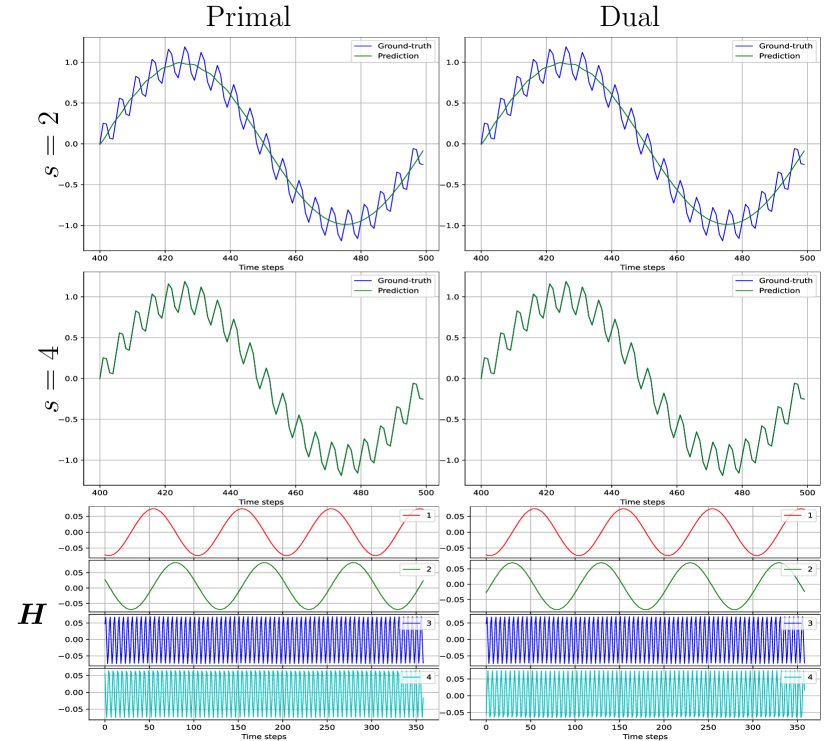
Figure 2: Forecasts (first two rows) and latent components (last row) obtained from the primal and dual models, trained by eigenvalue decomposition, with different number of components. Dataset: Sum of sine waves, $p=40$ and linear kernels on both views. Principal components ($\bm{H}\in\mathbb{R}^{n\times 4}$) obtained from training the primal (Equation 6) and dual models (Equation 13). These components are used progressively to obtain forecasts.

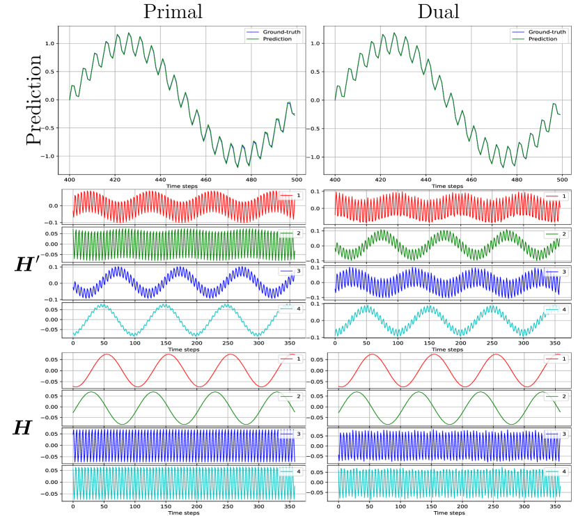
Figure 3: Forecasts (first row) and latent components (last two rows) obtained from the Stiefel training of primal and dual models on Sum of Sine waves dataset. See Corollaries 3.4 and 3.6 for obtaining $\bm{H}^{\prime}$ and $\bm{H}$.

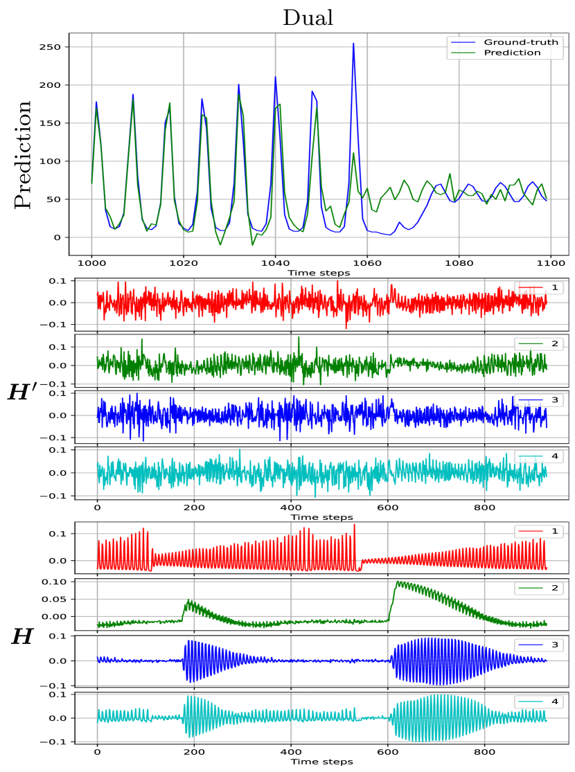
Figure 4: Forecasts ($1^{\text{st}}$ row) and latent components (last two rows) obtained from the Stiefel training of the dual model on SantaFe dataset. See Corollaries 3.4 and 3.6 for obtaining $\bm{H}^{\prime}$ and $\bm{H}$.

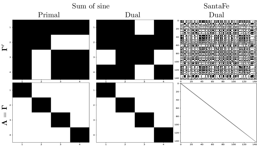
Figure 5: Illustration of the obtained $\bm{\Gamma}^{\prime}$ matrix of the models trained with the Stiefel optimizer, which contains many nonzero elements outside its diagonal. Their transformations $\bm{\Gamma}=\bm{\Gamma}^{\prime}\bm{O}$ equal the diagonal eigenvalue matrix $\bm{\Lambda}$ obtained by the eigendecomposition based algorithms (see Corollaries 3.4 and 3.6).

5 Experiments

In this section, we perform experiments on publicly available standard datasets to validate our proposed framework. In particular, we validate Algorithms 2, 1, 4 and 3 and the duality in the framework by analyzing the latent components $\bm{H}$ and the predictions $\bm{y}$. The code used to reproduce the experiments is provided on Github .

For simplicity and clarity, we consider two views ($V=2$), where one view is treated as the input source ($\mathcal{X}$) and the other view as the target ($\mathcal{Y}$) in the time series forecasting problem. We use this 2-view model as the static regression problem and build a Non-linear Autoregressive model $\hat{{x}}_{\ell+1}=f({x}_{\ell},{x}_{\ell-1},\ldots,{x}_{\ell-p})$ with lag parameter $p\in\mathbb{N}$ and $\hat{{y}}$ is the estimated output. Given a time-series of length $T$: $\{{x}_{\ell}\}_{\ell=1}^{T}$, we construct a training set with inputs $\bm{x}_{\ell}=x_{\ell:\ell-p}$ and corresponding outputs ${y}_{\ell}={x}_{\ell+1}$, with $\ell$ ranging from $p+1$ to $T-1$. During the prediction phase, the output from the previous time-step is used as input in the current step. This is used iteratively to forecast multiple steps ahead in future.

Sum of Sinusoids. We begin with a toy-experiment to better understand different components of the model. Consider this synthetic time-series of the sum of two sine waves: $x_{\ell}=\sum_{j=1}^{2}\alpha_{j}\sin(2\pi\omega_{j}\ell)$, $\alpha_{j}\in\{1,0.2\}$, $\omega_{j}\in\{100,2000\}$. We use linear kernels on both the views: $k_{{x}}(\cdot,\cdot)$ and $k_{{y}}(\cdot,\cdot)$. Since linear kernels are used, feature maps and hence the pre-image maps are identity functions. In this experiment, we test whether the embeddings in the latent space (also called as principal components) and the predictions are equivalent across all the Algorithms 2, 1, 4 and 3.

Figure 2 shows the forecasts and latent components when the primal and dual models are trained with eigenvalue decomposition. It also shows the ablation study of using the different number of components $s$ for prediction. The figure clearly shows that each component progressively captures more variance in the dataset.

Table 2: Experiment matrix for Sum of Sinusoids dataset

	Primal	Dual
Eig.	✓	✓
$\operatorname{\mathrm{St}}$	✓	✓

Further, the forecasts from both primal and dual models are identical. Another interesting observation is that the latent components are also equivalent up to a sign-flip. This corroborates the observation that the eigenvectors are unique up to a sign-flip.

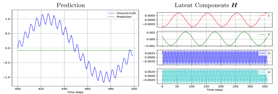
Figure 7: Forecasts and latent components obtained from the eigenvalue decomposition training of primal model on Sum of Sine waves dataset. This is done without scaling $\bm{U}$ as proposed in step 6 of Algorithm 1 i.e. setting $\bm{U}=\tilde{\bm{U}}$. Notice that the latent components are equivalent as in Figure 2 but only upto a scaling (and sign-flip). However on the predictions, this has a severely adverse effect and the model does not learn any variance in the dataset.

Significance of rescaling the primal variables. We repeated the above experiment in primal setting, while omitting step 6 in Algorithm 1. Figure 7 in Appendix C shows that the equivalence with the dual setting is only achieved up to a scaling for the dual components. Moreover, the figure also shows that omitting the rescaling has a detrimental effect on the predictions. This effect was not observed in Pandey et al. (2022b) because they trained a parametric pre-image map, combined with a reconstruction loss. Because of this, the rescaling was implicitly embedded in the pre-image map instead of the primal components themselves.

Next, we turn our attention to the Stiefel training of primal and dual models. See Figure 3 for the forecasts and the latent components as obtained by the Stiefel training $\bm{H}^{\prime}$ and rotated ones $\bm{H}$. Figure 5 shows an illustration of the obtained hyperparameter matrices in both cases. Note that such rotational transformations can always be obtained and are computationally easy to compute ($\mathcal{O}(s^{3})$). The figure shows the equivalence between both the models when trained with optimization on Stiefel manifold or when trained with eigenvalue decomposition in Figure 2 (ref. Table 2).

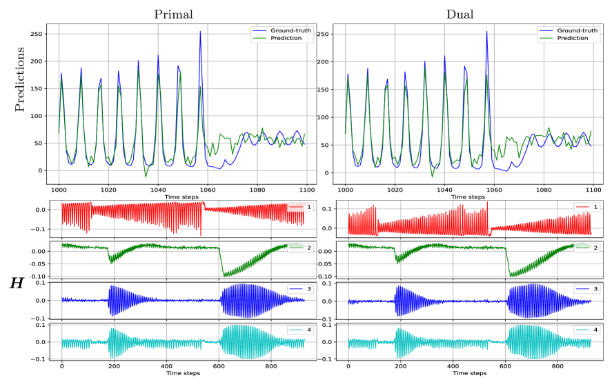
Figure 6: Forecasts ($1^{\text{st}}$ row) and top-4 latent components (last rows) obtained from the primal and dual model trained by eigenvalue decomposition. Dataset: SantaFe, $k_{x}$ is Gaussian kernel ($\sigma=2.1856$) approximated by Random Fourier Features ($d_{f,x}=5000$), $k_{y}$ is linear kernel, $p=70$, $s=144$.

SantaFe. We repeat the above experiments on a real-world chaotic time-series dataset: SantaFe (Weigend & Gershenfeld, 1993). Since the goal is to compare primal and dual models, the feature maps has to be explicitly known. Therefore, we use the Random Fourier Features ($d_{f,x}=5000$) as an approximation of the Gaussian kernel on $k_{x}$ and linear kernel on $k_{y}$. Since this linear kernel has identity feature map, no pre-image method is needed for predictions. Figure 6 in Appendix C shows the latent components and the predictions for the SantaFe dataset when the primal and dual models are trained with eigenvalue decomposition. We can see that the latent components and predictions are consistent with each other. We note that the goal of this experiment is not to have the best predictive performance, but to validate the duality in our model through different algorithms. Nevertheless, the predictive performance could be improved with further hyperparameter tuning.

Table 3: Experiment matrix for SantaFe dataset

	Primal	Dual
Eig.	✓	✓
$\operatorname{\mathrm{St}}$	—	✓

In the case of Stiefel training, by following the flowchart in Figure 1, we deduce that the Algorithm 4 is computationally efficient in this case. This is because of the comparatively smaller parameter matrix given by the dual formulation. Kernel matrix $\bm{K}\in\mathbb{R}^{n\times n}$, where $n=1000$ leads to a parameter matrix $\bm{H}\in\operatorname{\mathrm{St}}(1000,s)$. On the other hand, the covariance matrix $\bm{C}\in\mathbb{R}^{5001\times 5001}$ is quite large due to the very high-dimensional feature space ($d_{f,x}=5000$) given by the Random Fourier Features. This in turn, creates about 5 times larges parameter matrix for Stiefel optimization $\bm{U}\in\operatorname{\mathrm{St}}(5001,s)$. Therefore, cleverly using the duality helps us to obtain a computational speed gain of 5x in this case. Figure 4 shows the forecasts and latent components $\bm{H}^{\prime}$ and $\bm{H}$. By comparing it with Figure 6, we conclude that the duality holds not just in theory but also in practice (ref. Table 3).

Lastly, the role of Stiefel training becomes critical when training parametric feature/pre-image maps ($\phi_{v}(\cdot;\bm{\theta}),\psi_{v}(\cdot;\bm{\eta})$) such as deep neural networks where the parameter space is quite large. In such cases, it becomes computationally infeasible to perform matrix decomposition in every mini-batch of the training loop.

Given that previous studies Tonin et al. (2021b); Pandey et al. (2021; 2022b; 2023) have already benchmarked and demonstrated the soundness and effectiveness of individual algorithms, the primary objective of this paper is to enhance our understanding of the relationships between these methods, by assessing the equivalence of their core models. Therefore, we did not focus on performances and even judged that using models with sub-optimal performance are better to (visually) assess the equivalence.

6 Conclusion

We explored and highlighted duality in Multi-view Kernel PCA. Further, we provided a flowchart of four algorithms to train the models depending on whether the feature maps are known or not, whether they are parametric or not and the number of data-points versus the dimensionality of the feature spaces. By rescaling primal variables, we showed the equivalence of the primal and dual setting. We show how to rotate the solution obtained by Stiefel optimization based algorithms to match the components of the eigendecompositions. Lastly, we validated our model and algorithms on publicly available standard datasets and performed ablation studies where we empirically verified the equivalence. Future work includes investigating equivalence for generative modeling. Furthermore, how to enable mini-batch training in the dual formulation remains an open question.

Appendix A List of symbols

Symbol	Space	Description
$\bm{1}_{n}$	$\{1\}^{n}$	$n$-dimensional vector of all ones
$\boldsymbol{\Gamma}$	$\mathbb{R}_{\succ 0}^{s\times s}$	symmetric positive definite hyperparameter matrix
$\delta_{ij}$	$\{0,1\}$	Kronecker delta
$\boldsymbol{\eta}$	$\mathbb{R}^{t}$	parametervector of a parametric pre-image map with $t$ parameters
$\boldsymbol{\theta}$	$\mathbb{R}^{t}$	parametervector of a parametric feature map with $t$ parameters
$\boldsymbol{\Lambda}$	$\mathbb{R}_{\succ 0}^{s\times s}$	diagonal matrix containing eigenvalues
$\phi_{v}(\cdot)$	$\mathbb{R}^{d}\mapsto\mathbb{R}^{d_{f,v}}$	feature map for view $v$, transforming an input from a $d$-dimensional space to a $d_{f}$-dimensional space
$\Phi_{v}$	$\mathbb{R}^{n\times d_{f,v}}$	matrix containing all feature maps as row vectors
$\psi_{v}(\cdot)$	$\mathbb{R}^{d_{f,v}}\mapsto\mathbb{R}^{d_{v}}$	pre-image map of view $v$ $\psi_{v}(\cdot)\equiv\phi_{v}^{-1}(\cdot)$
$\bm{C}$	$\mathbb{R}^{d_{f}\times d_{f}}$	cross-covariance matrix (see (10))
$\bm{C}_{vw}$	$\mathbb{R}^{d_{f,v}\times d_{f,w}}$	cross-covariance matrix of views $v$ and $w$
$d_{f}$	$\mathbb{N}$	sum of feature space dimensionalities of all views
$d_{f,v}$	$\mathbb{N}$	feature space dimensionality of view $v$
$d_{v}$	$\mathbb{N}$	input space dimensionality of view $v$
$\bm{e}_{v,i}$	$\mathbb{R}^{s}$	score variable of datapoint $i$ for view $v$
$\bm{h}_{i}$	$\mathbb{R}^{s}$	dual representation of datapoint $i$
$\bm{H}$	$\mathbb{R}^{n\times s}$	matrix containing all dual representations as row vectors
$\mathbb{I}_{n}$	$\{0,1\}^{n\times n}$	$n$ by $n$ identity matrix
$k_{v}(\cdot,\cdot)$	$\mathbb{R}^{d_{v}}\times\mathbb{R}^{d_{v}}\mapsto\mathbb{R}$	a positive definite kernel function
$\bm{K}$	$\mathbb{R}^{n\times n}$	summation of all $\bm{K}_{v}$
$\bm{K}_{v}$	$\mathbb{R}^{n\times n}$	kernel matrix $K_{v,ij}=k(\bm{x}_{v,i},\bm{x}_{v,j})$, or the Gram matrix $K_{v,ij}=\langle\phi_{v}(\bm{x}_{v,i}),\phi_{v}(\bm{x}_{v,j})\rangle_{\mathcal{H}}$ for view $v$
$\ell$	$\mathbb{N}$	timestep index of timeseries
$\bm{M}_{c}$	$\mathbb{R}^{n\times n}$	centering matrix, used to center the kernel matrix
$n$	$\mathbb{N}$	number of datapoints
$p$	$\mathbb{N}$	number of lags
$s$	$\mathbb{R}$	dimensionality of the score variables and dual representations, i.e., number of components
$\bm{U}$	$\mathbb{R}^{d_{f}\times s}$	concatenation of all $\bm{U}_{v}$
$\bm{U}_{v}$	$\mathbb{R}^{d_{f,v}\times s}$	linear transformation matrix for view $v$
$V$	$\mathbb{N}$	number of views (data modalities)
$\bm{x}_{v,i}$	$\mathbb{R}^{d_{v}}$	the feature vector of datapoint $i$ for view $v$
${y}_{i}$	$\mathbb{R}$	target variable of datapoint $i$
$\bm{Z}$	$\mathbb{R}^{s\times s}$	a matrix containing Lagrange multipliers

Appendix B Proofs

B.1 Proof of Lemma 3.2

Proof.

By eliminating dual variables $\bm{h}_{i}$ from (5) using (6), one obtains:

$$\sum_{w=1}^{V}\bm{C}_{vw}\bm{U}_{w}=\bm{U}_{v}\bm{\Gamma},\quad\forall v,$$ (17)

and by substituting (6) in (7):

$$\phi_{v}(\bm{x}_{v,i})=\bm{U}_{v}\bm{\Gamma}^{-1}\sum_{w=1}^{V}\bm{U}_{w}^{\top}\phi_{w}(\bm{x}_{w,i}).$$ (18)

Next, the Lagrangian of (8) is:

$$\mathcal{L}(\tilde{\bm{U}},\bm{Z})=J_{\text{pr}}+\frac{1}{2}\operatorname{\mathrm{Tr}}\left(\bm{Z}^{\top}\left(-\mathbb{I}_{s}+\sum_{v=1}^{V}\tilde{\bm{U}}_{v}^{\top}\tilde{\bm{U}}_{v}\right)\right),$$

and the Karush-Kuhn-Tucker conditions are:

$$\dfrac{\partial\mathcal{L}}{\partial\tilde{\bm{U}}_{v}}=0\Rightarrow \ \sum_{w=1}^{V}\bm{C}_{vw}\tilde{\bm{U}}_{w}=\tilde{\bm{U}}_{v}\tilde{\bm{Z}}, \forall v,$$ (19)

$$\dfrac{\partial\mathcal{L}}{\partial\phi_{v}(\bm{x}_{v,i})}=0\Rightarrow \ \phi_{v}(\bm{x}_{v,i})=\tilde{\bm{U}}_{v}\sum_{w=1}^{V}\tilde{\bm{U}}_{w}^{\top}\phi_{w}(\bm{x}_{w,i}), \forall v,i$$ (20)

$$\dfrac{\partial\mathcal{L}}{\partial\bm{Z}}=0\Rightarrow \ \sum_{v=1}^{V}\tilde{\bm{U}}_{v}^{\top}\tilde{\bm{U}}_{v}=\mathbb{I}_{s}, \forall v.$$ (21)

By replacing $\tilde{\bm{U}}_{v}$ in the KKT conditions with $\bm{U}_{v}\tilde{\bm{Z}}^{-1/2}$, and by choosing $\bm{\Gamma}=\tilde{\bm{Z}}$, we obtain (17) and (18) from (19) and (20) respectively, which proves the Lemma. ∎

B.2 Proof of Proposition 3.3

We use the proof as given by Achten et al. (2023, Appendix), and rewrite it for the variables $\bm{A}=[\bm{a}_{1},\dots,\bm{a}_{m}]^{\top}$ and $\bm{B}$.

Proof.

The Lagrangian of (3.3) is:

$$\mathcal{L}(\bm{A},\bm{Z})=-\frac{1}{2}\text{Tr}(\bm{A}^{\top}\bm{B}\bm{A})+\frac{1}{2}\text{Tr}(\bm{B})+\frac{1}{2}\text{Tr}(\bm{Z}^{\top}(\bm{A}^{\top}\bm{A}-\mathbb{I}_{n})),$$

and the Karush-Kuhn-Tucker conditions are:

$$\left\{\begin{array}[]{l}\frac{\partial\mathcal{L}}{\partial\bm{A}}=-\bm{B}\bm{A}+\bm{A}(\bm{Z}+\bm{Z}^{\top})/2=0\\ \\ \frac{\partial\mathcal{L}}{\partial\bm{Z}}=\bm{A}^{\top}\bm{A}-\mathbb{I}_{n}=\bm{0}_{n}.\end{array}\right.$$ (22)

Let us define the columns of $\bm{A}$ as $\bm{g}_{i}=[(\bm{a}_{1})_{i},\dots,(\bm{a}_{m})_{i}]^{\top}$, and $\bm{G}=[\bm{g}_{1},\dots,\bm{g}_{n}]=\bm{A}$. By also defining $\tilde{\bm{Z}}=(\bm{Z}+\bm{Z}^{\top})/2$, we can then rewrite (22) in vector notation:

$$\left\{\begin{array}[]{l}\frac{\partial\mathcal{L}}{\partial\bm{g}_{i}}=-\frac{1}{\eta}\bm{B}\bm{g}_{i}+\sum_{j=1}^{n}\tilde{Z}_{ij}\bm{g}_{j}=\bm{0}_{m}\quad\forall i=1\dots n\\ \\ \frac{\partial\mathcal{L}}{\partial\tilde{Z}_{ij}}=\bm{g}_{i}^{\top}\bm{g}_{j}-\delta_{ij}=0\quad\forall i,j=1\dots n\end{array}\right.$$ (23)

where $\delta_{ij}$ is the Kronecker delta, and derive the second order derivatives for the optimization parameters:

$$\nabla^{2}_{\bm{g}_{i}\bm{g}_{j}}\mathcal{L}=-\frac{\delta_{ij}}{\eta}\bm{B}+\tilde{Z}_{ij}\mathbb{I}_{m}.$$ (24)

By defining $\bm{D}=[\bm{d}_{1},\dots,\bm{d}_{n}]$, the second order necessary conditions can be formulated as:

$$\sum_{i=1}^{n}\sum_{j=1}^{n}\bm{d}_{i}^{\top}(-\frac{\delta_{ij}}{\eta}\bm{B}+\tilde{Z}_{ij}\mathbb{I}_{m})\bm{d}_{j}=-\frac{1}{\eta}\sum_{i=1}^{n}\bm{d}_{i}^{\top}\bm{B}\bm{d}_{i}+\sum_{i=1}^{n}\sum_{j=1}^{n}\tilde{Z}_{ij}\bm{d}_{i}^{\top}\bm{d}_{j}\geq 0$$

$$\forall\bm{D}\in C(\bm{G}^{*}),$$ (25)

where $C(\bm{G}^{*})=\{\bm{D}\in\mathbb{R}^{m\times n}\ |\ \bm{D}^{\top}\bm{G}^{*}=\bm{0}_{n}\}$ is the critical cone at $\bm{G}^{*}$. For the critical cone, it can be deduced that the following properties hold:

$$\bm{d}_{i}^{\top}\bm{g}^{*}_{j}+\bm{d}_{j}^{\top}\bm{g}^{*}_{i}=0 \quad\forall i,j=1,\dots,n$$

$$\bm{d}_{i}^{\top}\bm{g}^{*}_{i}=0 \quad\forall i=1,\dots,n$$

$$\bm{d}_{i}^{\top}\bm{d}_{j}=0 \quad\forall i,j=1,\dots,n\quad i\neq j.$$

Without loss of generality, we further assume $\lVert\bm{d}_{i}\rVert=1$. From (23), one can derive $\tilde{Z}_{ij}=\frac{1}{\eta}\bm{g}^{*\top}_{j}\bm{B}\bm{g}^{*}_{i}$. By substituting this and $\bm{d}_{i}^{\top}\bm{d}_{j}=0$ in (25), the second order necessary condition becomes:

$$\sum_{i=1}^{n}\frac{1}{\eta}\bm{g}^{*\top}_{i}\bm{B}\bm{g}^{*}_{i}\geq\sum_{i=1}^{n}\frac{1}{\eta}\bm{d}_{i}^{\top}\bm{B}\bm{d}_{i},$$

or after reworking this algebraically:

$$\text{Tr}(\bm{G}^{*\top}\bm{V}\boldsymbol{\Lambda}\bm{V}^{\top}\bm{G}^{*})\geq\text{Tr}(\bm{D}^{\top}\bm{V}\boldsymbol{\Lambda}\bm{V}^{\top}\bm{D}),$$ (26)

with $\bm{V}=[\bm{v}_{1},\dots,\bm{v}_{m}]$ the eigenvectors of $\bm{B}$ with corresponding eigenvalues $\boldsymbol{\Lambda}=\text{diag}(\lambda_{1},\dots,\lambda_{m})$. For the case where $\text{span}(\bm{g}^{*}_{1},\dots,\bm{g}^{*}_{n})=\text{span}(\bm{v}_{1},\dots,\bm{v}_{n})$, the left hand side is maximal:

$$\sum_{i=1}^{n}\lambda_{i}=\text{Tr}(\bm{G}^{*\top}\bm{V}\boldsymbol{\Lambda}\bm{V}^{\top}\bm{G}^{*})\geq\text{Tr}(\bm{D}^{\top}\bm{V}\boldsymbol{\Lambda}\bm{V}^{\top}\bm{D}).$$

The right hand side becomes maximal when $\text{span}(\bm{d}_{1},\dots,\bm{d}_{n})=\text{span}(\bm{v}_{1},\dots,\bm{v}_{n})$. In this case, there exists an orthonormal transformation matrix $\bm{O}$ such that $\bm{G}^{*}=\bm{D}\bm{O}$:

$$\sum_{i=1}^{n}\lambda_{i}=\text{Tr}(\bm{G}^{*\top}\bm{V}\boldsymbol{\Lambda}\bm{V}^{\top}\bm{G}^{*})=\text{Tr}(\bm{O}^{\top}\bm{D}^{T}\bm{V}\boldsymbol{\Lambda}\bm{V}^{\top}\bm{D}\bm{O})=\text{Tr}(\bm{D}^{\top}\bm{V}\boldsymbol{\Lambda}\bm{V}^{\top}\bm{D}).$$

We verified that the second order necessary conditions are satisfied for in the case $\text{span}(\bm{g}^{*}_{1},\dots,\bm{g}^{*}_{n})=\text{span}(\bm{v}_{1},\dots,\bm{v}_{n})$. Let us now proceed by assuming that $\text{span}(\bm{g}^{*}_{1},\dots,\bm{g}^{*}_{n})\neq\text{span}(\bm{v}_{1},\dots,\bm{v}_{n})$. In this case there exists a matrix $\bm{D}$ such that (26) becomes:

$$\text{Tr}(\bm{G}^{*\top}\bm{V}\boldsymbol{\Lambda}\bm{V}^{\top}\bm{G}^{*})<\text{Tr}(\bm{D}^{\top}\bm{V}\boldsymbol{\Lambda}\bm{V}^{\top}\bm{D})\leq\sum_{i=1}^{n}\lambda_{i}.$$

We thus established that the second order necessary conditions are satisfied if and only if $\text{span}(\bm{g}^{*}_{1},\dots,\bm{g}^{*}_{n})=\text{span}(\bm{v}_{1},\dots,\bm{v}_{n})$. Generally, the second order condition is not sufficient. However, as the feasible set $\{\bm{A}\in\mathbb{R}^{m\times n}\ |\ \bm{A}^{\top}\bm{A}-\mathbb{I}_{n}=\bm{0}_{n}\}$ is compact, and the objective function $-\frac{1}{2}\text{Tr}(\bm{A}^{\top}\bm{B}\bm{A})+\text{Tr}(\bm{B})$ is concave, (3.3) is guaranteed to have a global minimizer Boyd & Vandenberghe (2004). Therefore, any $\bm{A}^{*}$ such that $\text{range}(\bm{A}^{*})=span(\bm{v}_{1}\dots\bm{v}_{n})$ is a global minimizer.

∎

B.3 Proof of Lemma 3.5

Proof.

By eliminating primal variables $\bm{U}_{v}$ from (6) using (5), one obtains:

$$\bm{K}\bm{H}=\bm{H}\bm{\Gamma},$$ (27)

where $\bm{K}=\sum_{v=1}^{V}\bm{K}_{v}$, and by substituting (5) in (7):

$$\phi_{v}(\bm{x}_{v,i})=\sum_{j=1}^{n}\phi_{v}(\bm{x}_{v,j})\bm{h}_{j}^{\top}\bm{h}_{i}.$$ (28)

Next, the Lagrangian of (12) is:

$$\mathcal{L}({\bm{H}},\bm{Z})=J_{\text{d}}+\frac{1}{2}\operatorname{\mathrm{Tr}}\left(\bm{Z}^{\top}\left(-\mathbb{I}_{s}+{\bm{H}}^{\top}{\bm{H}}\right)\right),$$

and the Karush-Kuhn-Tucker conditions are:

$$\dfrac{\partial\mathcal{L}}{\partial{\bm{H}}}=0\Rightarrow\ [\sum_{v=1}^{V}\bm{K}_{v}]{\bm{H}}={\bm{H}}\tilde{\bm{Z}}$$ (29)

$$\dfrac{\partial\mathcal{L}}{\partial\phi_{v}(\bm{x}_{v,i})}=0\Rightarrow\ \phi_{v}(\bm{x}_{v,i})=\sum_{j=1}^{n}\phi_{v}(\bm{x}_{v,j})\bm{h}_{j}^{\top}\bm{h}_{i}$$ (30)

$$\dfrac{\partial\mathcal{L}}{\partial\bm{Z}}=0\Rightarrow \ {\bm{H}}^{\top}{\bm{H}}=\mathbb{I}_{s}.$$ (31)

By choosing $\bm{\Gamma}=\tilde{\bm{Z}}$, we obtain (27) from (29). Since also (28) equals (30), we have proven the Lemma. ∎

Appendix C Datasets and additional experiments

We refer to Table 4 for more details on model architectures, datasets and hyperparameters used in this paper. The PyTorch library (double precision) in Python was used. See Algorithms 2, 1, 4 and 3 for training the MV-RKM model.

Table 4: Datasets used for the experiments. $n_{\text{train}}$, $n_{\text{test}}$ is the number of training and test samples respectively, $d$ the time series dimension, $p$ is the lag, $s$ is the latent space dimension, RFF and RBF mean ’random Fourier features’ and ’radial basis function’ respectively.

Dataset	$n_{\text{train}}$	$n_{\text{test}}$	$d$	$p$	$\phi_{x}$	$k_{x}$	$\phi_{y}$	$k_{y}$	$s$
Sum of Sine	400	100	1	40	Linear	Linear	Linear	Linear	4
SantaFe	1000	100	1	70	RFF	RBF	Linear	Linear	144

References

- Achten et al. (2023) Achten, S., Tonin, F., Patrinos, P., and Suykens, J. A. K. Semi-Supervised Classification with Graph Convolutional Kernel Machines, 2023. arXiv:2301.13764 [cs].
- Alaíz et al. (2018) Alaíz, C. M., Fanuel, M., and Suykens, J. A. K. Convex formulation for Kernel PCA and its use in semisupervised learning. IEEE Transactions on Neural Networks and Learning Systems, 29(8):3863–3869, 2018. doi: 10.1109/TNNLS.2017.2709838.
- Boyd & Vandenberghe (2004) Boyd, S. and Vandenberghe, L. Convex Optimization. Cambridge University Press, New York, NY, USA, 2004. ISBN 0521833787.
- Bui et al. (2019) Bui, A. T., Im, J.-K., Apley, D. W., and Runger, G. C. Projection-free kernel principal component analysis for denoising. Neurocomputing, 357:163–176, 2019. ISSN 0925-2312. doi: https://doi.org/10.1016/j.neucom.2019.04.042.
- Gao et al. (2020) Gao, J., Li, P., Chen, Z., and Zhang, J. A Survey on Deep Learning for Multimodal Data Fusion. Neural Computation, 32(5):829–864, 05 2020. ISSN 0899-7667. doi: 10.1162/neco˙a˙01273. URL https://doi.org/10.1162/neco_a_01273.
- Gönen & Alpaydın (2011) Gönen, M. and Alpaydın, E. Multiple kernel learning algorithms. The Journal of Machine Learning Research, 12:2211–2268, 2011.
- Guo et al. (2014) Guo, D., Zhang, J., Liu, X., Cui, Y., and Zhao, C. Multiple kernel learning based multi-view spectral clustering. In 2014 22nd International Conference on Pattern Recognition, pp. 3774–3779, 2014. doi: 10.1109/ICPR.2014.648.
- Hinton (2005) Hinton, G. E. What kind of a graphical model is the brain? In Proceedings of the 19th International Joint Conference on Artificial Intelligence, IJCAI’05, pp. 1765–1775, San Francisco, CA, USA, 2005. Morgan Kaufmann Publishers Inc.
- Honeine & Richard (2011) Honeine, P. and Richard, C. Preimage problem in kernel-based machine learning. IEEE Signal Processing Magazine, 28(2):77–88, March 2011. ISSN 1053-5888.
- Houthuys & Suykens (2021) Houthuys, L. and Suykens, J. A. Tensor-based restricted kernel machines for multi-view classification. Information Fusion, 68:54–66, 2021. ISSN 1566-2535. doi: https://doi.org/10.1016/j.inffus.2020.10.022.
- Kwok & Tsang (2003) Kwok, J. T. and Tsang, I. W.-H. The pre-image problem in kernel methods. IEEE Transactions on Neural Networks, 15:1517–1525, 2003.
- LeCun et al. (2006) LeCun, Y., Chopra, S., Hadsell, R., Ranzato, M., and Huang, F. A tutorial on energy-based learning. Predicting structured data, 1(0), 2006.
- Li et al. (2019) Li, J., Li, F., and Todorovic, S. Efficient Riemannian Optimization on the Stiefel Manifold via the Cayley Transform. In ICLR, 2019.
- Mika et al. (1999a) Mika, S., Ratsch, G., Weston, J., Schölkopf, B., and Müller, K. R. Fisher discriminant analysis with kernels. In Neural Networks for Signal Processing IX: Proceedings of the 1999 IEEE Signal Processing Society Workshop (Cat. No.98TH8468), pp. 41–48, 1999a. doi: 10.1109/NNSP.1999.788121.
- Mika et al. (1999b) Mika, S., Schölkopf, B., Smola, A., Müller, K.-R., Scholz, M., and Rätsch, G. Kernel pca and de-noising in feature spaces. In Advances in Neural Information Processing Systems, pp. 536–542. MIT Press, 1999b.
- Pandey et al. (2021) Pandey, A., Schreurs, J., and Suykens, J. A. Generative restricted kernel machines: A framework for multi-view generation and disentangled feature learning. Neural Networks, 135:177–191, 2021.
- Pandey et al. (2022a) Pandey, A., De Meulemeester, H., De Plaen, H., De Moor, B., and Suykens, J. Recurrent Restricted Kernel Machines for Time-series Forecasting. In ESANN 2022 proceedings, pp. 399–404, Bruges (Belgium) and online event, 2022a. ISBN 978-2-87587-084-1. doi: 10.14428/esann/2022.ES2022-120.
- Pandey et al. (2022b) Pandey, A., Fanuel, M., Schreurs, J., and Suykens, J. A. K. Disentangled representation learning and generation with manifold optimization. Neural Computation, 34(10):2009–2036, 09 2022b. ISSN 0899-7667. doi: 10.1162/neco˙a˙01528.
- Pandey et al. (2023) Pandey, A., De Meulemeester, H., De Moor, B., and Suykens, J. A. K. Multi-view Kernel PCA for Time series Forecasting, January 2023. arXiv:2301.09811 [cs].
- Rahimi & Recht (2007) Rahimi, A. and Recht, B. Random features for large-scale kernel machines. In Platt, J., Koller, D., Singer, Y., and Roweis, S. (eds.), Advances in Neural Information Processing Systems, volume 20. Curran Associates, Inc., 2007.
- Rasmussen & Williams (2006) Rasmussen, C. E. and Williams, C. K. I. Gaussian processes for machine learning. Adaptive computation and machine learning. MIT Press, 2006. ISBN 026218253X.
- Rockafellar (1974) Rockafellar, R. T. Conjugate Duality and Optimization. Society for Industrial and Applied Mathematics, 1974. doi: 10.1137/1.9781611970524.
- Salakhutdinov & Hinton (2009) Salakhutdinov, R. and Hinton, G. Deep Boltzmann Machines. In van Dyk, D. and Welling, M. (eds.), Proceedings of the Twelth International Conference on Artificial Intelligence and Statistics, volume 5 of Proceedings of Machine Learning Research, pp. 448–455, Hilton Clearwater Beach Resort, Clearwater Beach, Florida USA, 16–18 Apr 2009. PMLR.
- Salakhutdinov et al. (2007) Salakhutdinov, R., Mnih, A., and Hinton, G. Restricted Boltzmann Machines for collaborative filtering. In ICML ’07, pp. 791–798, Corvalis, Oregon, 2007. ACM Press.
- Schölkopf & Smola (2001) Schölkopf, B. and Smola, A. J. Learning with Kernels: Support Vector Machines, Regularization, Optimization, and Beyond. MIT Press, Cambridge, MA, USA, 2001. ISBN 0262194759.
- Schölkopf et al. (1998) Schölkopf, B., Smola, A., and Müller, K.-R. Nonlinear Component Analysis as a Kernel Eigenvalue Problem. Neural Computation, 10(5):1299–1319, 1998. doi: 10.1162/089976698300017467.
- Schreurs & Suykens (2018) Schreurs, J. and Suykens, J. A. K. Generative Kernel PCA. In European Symposium on Artificial Neural Networks, Computational Intelligence and Machine Learning , pp. 129–134, 2018.
- Suykens et al. (2003) Suykens, J., Van Gestel, T., Vandewalle, J., and De Moor, B. A support vector machine formulation to pca analysis and its kernel version. IEEE Transactions on Neural Networks, 14(2):447–450, 2003. doi: 10.1109/TNN.2003.809414.
- Suykens (2017) Suykens, J. A. K. Deep restricted kernel machines using conjugate feature duality. Neural Computation, 29(8):2123–2163, August 2017. ISSN 0899-7667, 1530-888X.
- Suykens et al. (2002) Suykens, J. A. K., Van Gestel, T., De Brabanter, J., De Moor, B., and Vandewalle, J. Least Squares Support Vector Machines. World Scientific, River Edge, NJ, January 2002. ISBN 978-981-238-151-4.
- Tonin et al. (2021a) Tonin, F., Pandey, A., Patrinos, P., and Suykens, J. A. K. Unsupervised energy-based out-of-distribution detection using stiefel-restricted kernel machine. In 2021 International Joint Conference on Neural Networks (IJCNN), pp. 1–8, 2021a. doi: 10.1109/IJCNN52387.2021.9533706.
- Tonin et al. (2021b) Tonin, F., Patrinos, P., and Suykens, J. A. Unsupervised learning of disentangled representations in deep restricted kernel machines with orthogonality constraints. Neural Networks, 142:661–679, 2021b. ISSN 0893-6080. doi: https://doi.org/10.1016/j.neunet.2021.07.023.
- Tonin et al. (2023) Tonin, F., Tao, Q., Patrinos, P., and Suykens, J. A. K. Deep kernel principal component analysis for multi-level feature learning, 2023.
- Vapnik (1995) Vapnik, V. N. The nature of statistical learning theory. Springer-Verlag New York, Inc., 1995. ISBN 0-387-94559-8.
- Weigend & Gershenfeld (1993) Weigend, A. and Gershenfeld, N. Time Series Prediction: Forecasting the Future and Understanding the Past. Addison-Wesley, 1993.
- Weston et al. (2003) Weston, J., Schölkopf, B., and Bakir, G. Learning to find pre-images. In Advances in Neural Information Processing Systems, volume 16, 2003.
- Williams & Seeger (2000) Williams, C. and Seeger, M. Using the Nyström method to speed up kernel machines. In Leen, T., Dietterich, T., and Tresp, V. (eds.), Advances in Neural Information Processing Systems, volume 13. MIT Press, 2000.
- Winant et al. (2020) Winant, D., Schreurs, J., and Suykens, J. A. K. Latent space exploration using generative kernel PCA. In Bogaerts, B., Bontempi, G., Geurts, P., Harley, N., Lebichot, B., Lenaerts, T., and Louppe, G. (eds.), Artificial Intelligence and Machine Learning, pp. 70–82, Cham, 2020. Springer International Publishing.