Bilipschitz group invariants

Abstract

Consider the quotient of a real Hilbert space by a subgroup of its orthogonal group. We study whether this orbit space can be embedded into a Hilbert space by a bilipschitz map, and we identify constraints on such embeddings.

1 Introduction

Given a real Hilbert space $V$ and a subgroup $G$ of the orthogonal group $O(V)$, we wish to embed the orbit space $V/G:=\{G\cdot x:x\in V\}$ into a Hilbert space by a bilipschitz map. We are motivated by the analysis of data that resides in such an orbit space. For example:

Graphs. The adjacency matrix of an unlabeled graph on $n$ vertices is a member of $\mathbb{R}^{n\times n}$, but this matrix representation is only unique up to the conjugation action of $S_{n}$.

Point clouds. A point cloud consisting of $n$ vectors in $\mathbb{R}^{d}$ can be represented as a member of $\mathbb{R}^{d\times n}$ up to the right action of $S_{n}$ (i.e., column permutation).

Landmarks. Landmarks of a biological specimen can be represented in $\mathbb{R}^{3\times n}$, with the left action of $SO(3)$ giving different representations of the same specimen.

Audio signals. An audio signal can be modeled as a real-valued function in $L^{2}(\mathbb{R})$, but different time delays of the same signal arise from an orthogonal action of $\mathbb{R}$.

In each of the settings above, data is represented in a real Hilbert space $V$, but each data point is naturally identified with the other members of its $G$-orbit. To correctly measure distance, it is more appropriate to treat the data as residing in the orbit space $V/G$. However, most of the existing data processing algorithms were designed for data in a Hilbert space, not an orbit space. The following section shows how a bilipschitz embedding of the orbit space into a Hilbert space will enable one to use such algorithms. Next, Section 3 defines the metric quotient $V//G$, whose points are the topological closures of $G$-orbits in $V$. This matches the intuition that salient features are continuous functions of the data; also, while $V/G$ might only be a pseudometric space, $V//G$ is always a metric space. Section 4 shows how a bilipschitz invariant on the sphere can be extended to a bilipschitz invariant on the entire space. In Section 5, we show that every bilipschitz invariant map is not differentiable. This represents a significant departure from classical invariant theory [54, 73, 80, 11], which studies polynomial (hence differentiable) invariants. Section 6 then uses the extension from Section 4 to construct bilipschitz invariants for finite $G\leq O(d)$ from bilipschitz polynomial invariants on the sphere, which in turn exist precisely when $G$ acts freely on the sphere (hence rarely). In Section 7, we use the semidefinite program from [64] to show that some of our extensions of polynomial invariants deliver the minimum possible distortion of $V//G$ into a Hilbert space. Finally, Sections 8 and 9 estimate the Euclidean distortion of infinite-dimensional Hilbert spaces modulo permutation and translation groups, respectively.

1.1 Related work

The literature considers many ways of processing data in an orbit space. In what follows, we discuss some relevant examples, which we broadly categorize according to their inspiration.

1.1.1 Deep learning

Much of today’s excitement in machine learning comes on the heels of deep neural networks achieving super-human performance in various tasks. For data with translation invariance, such as images and audio signals, it is empirically beneficial for the early layers of a neural network to exhibit convolutional structure [79, 36, 61, 51]. Since convolutions are equivariant to translation, one might think of these early layers as isolating translation-equivariant features of the data. The real-world success of convolutional neural networks inspired the development of more principled versions of this fundamental idea. For example, Mallat introduced the scattering transform [67, 23, 24, 85], which iteratively alternates between taking a wavelet decomposition and a pointwise absolute value. The scattering transform is invariant to translation and stable to diffeomorphism, and it has since been generalized to other settings [48, 74, 34].

A modern goal in this vein is to develop deep learning tools to accommodate non-Euclidean data, such as data in orbit spaces. This is the charge of geometric deep learning [22, 21]. As an example, consider the task of classifying molecules according to whether they are harmful to humans. We can represent the molecule as a graph, with vertices representing atoms and edges representing bonds, and then we can train a graph neural network for this classification task. By design, graph neural networks are invariant to relabeling the vertices of the input graph. As such, they either fail to separate certain pairs of non-isomorphic graphs, or they are slow (assuming the graph isomorphism problem is hard). The standard message-passing graph neural networks distinguish isomorphism classes of graphs as well as the Weisfeiler–Leman test [88, 92, 78, 57], while other approaches achieve better separation [70, 20, 56].

1.1.2 Invariant theory

One may express any group-invariant classifier as the composition of a group-invariant feature map with a classifier on the feature domain. The feature map is most expressive if it separates all pairs of distinct orbits. Such a map is known as a separating invariant. Under mild conditions on the group (e.g., if the group is finite), Hilbert [54] showed that there exists a polynomial map into finite-dimensional space that separates the orbits; in fact, one may take the coordinate functions to be generators of the algebra of invariant polynomials. Modern work in invariant theory constructs smaller separating sets of polynomials with bounds on their degrees [42, 39, 40, 41]. Such polynomial maps play a key role in both invariant and equivariant machine learning [82, 83, 18].

Polynomial invariants are also used to solve the orbit recovery problem. For this problem, there is a known group $G$ acting linearly on a vector space $V$, and the task is to recover the orbit $G\cdot x$ of an unknown point $x\in V$ from data of the form $\{y_{i}=g_{i}x+e_{i}\}_{i=1}^{n}$, where each $g_{i}\in G$ and $e_{i}\in V$ is drawn independently at random. (In some settings, this problem is also known as multi-reference alignment and can be viewed as a sub-problem of cryo-electron microscopy.) Much of the recent work on this problem applies the method of moments, where one uses the data to estimate the moment $m_{k}(x):=\mathbb{E}_{g\sim\operatorname{Unif}(G)}(gx)^{\otimes k}$ for various $k$, and then estimates the orbit $G\cdot x$ from these moments [11, 75, 17, 16, 44]. Notably, the coordinates of $m_{k}(x)$ are $G$-invariant polynomials of $x$.

Polynomial invariants have been investigated for well over a century, and the large body of existing work makes them particularly nice to interact with in theory. Unfortunately, they can be rather finicky in practice. As an example, consider the Viète map, which sends any tuple $\{a_{i}\}_{i=1}^{n}$ of complex numbers to the coefficients of the corresponding degree-$n$ monic polynomial $\prod_{i=1}^{n}(z-a_{i})$. This defines a homeomorphism $\mathbb{C}^{n}/S_{n}\to\mathbb{C}^{n}$ with the elementary symmetric polynomials as coordinate functions [89]. While the continuity of the inverse map is most cumbersome to demonstrate where the polynomial has repeated roots, the inverse map is also unstable elsewhere, perhaps most famously at Wilkinson’s polynomial $\prod_{k=1}^{20}(z-k)$ [90]. For this polynomial, perturbing the coefficient of $z^{19}$ by machine precision produces a sizable error in several of the roots. Considering we are motivated by computational applications, this suggests that we pursue a more stable family of invariants.

1.1.3 Phase retrieval

Consider the problem of recovering a vector $x\in\mathbb{C}^{d}$ from data of the form $\{y_{i}=|\langle a_{i},x\rangle|\}_{i=1}^{n}$. This is known as (generalized) phase retrieval. Note that the map $x\mapsto\{|\langle a_{i},x\rangle|\}_{i=1}^{n}$ is $G$-invariant, where $G=\{\lambda I_{d}:\lambda\in\mathbb{C},|\lambda|=1\}$. Over the last decade, researchers have investigated conditions under which this map separates orbits [8, 46, 19, 37, 84] and in a stable way [12, 10]. In addition, there are now several algorithms to invert this invariant map using semidefinite programming [29, 31, 38, 86, 50], combinatorics [2, 13], and non-convex optimization [30, 33, 81].

The theory that was developed to study this particular family of invariants has recently inspired the construction of new families of invariants for many more group actions. For example, [27, 26] modified polynomial separating invariants for abelian groups in order to be Lipschitz, [9] identified bilipschitz permutation invariants based on sorting, and [43, 3] discovered semialgebraic separating invariants for a variety of groups. Finally, [28, 68, 69] introduced and studied max filtering, which directly generalizes phase retrieval to produce easy-to-compute semialgebraic separating invariants for any closed group. Furthermore, max filtering invariants are frequently bilipschitz in the quotient metric, thereby avoiding the stability problem exemplified by Wilkinson’s polynomial.

1.1.4 Metric embeddings

Consider the following fundamental question: Given metric spaces $M$ and $N$, does there exist a bilipschitz map $M\to N$, i.e., a metric embedding of $M$ into $N$? This is an active area of research; see [72] for example. In the cases where a metric embedding exists, one seeks metric embeddings of minimal distortion, that is, the quotient of upper and lower Lipschitz bounds. If $M$ is finite and $N$ is $|M|$-dimensional Euclidean space, the distortion-minimizing embeddings can be determined by semidefinite programming [64, 65]. Building on ideas from [59], Eriksson-Bique [45] constructed a metric embedding of $\mathbb{R}^{d}/G$ for any finite $G\leq O(d)$ into a Euclidean space. Furthermore, the dimension of the target space and the distortion of the map are both bounded by functions of $d$. Note that any metric embedding $\mathbb{R}^{d}/G\to\mathbb{R}^{n}$ determines a $G$-invariant map $\mathbb{R}^{d}\to\mathbb{R}^{n}$ that separates $G$-orbits in a stable way. To date, Eriksson-Bique’s map and max filtering are the only known methods of constructing bilipschitz invariants for arbitrary finite subgroups of $O(d)$.

2 Bilipschitz maps and their applications

Given a map $f\colon X\to Y$ between metric spaces $X$ and $Y$, then provided $X$ has at least two points, we may take $\alpha,\beta\in[0,\infty]$ to be the largest and smallest constants (respectively) such that

$$\alpha\cdot d_{X}(x,x^{\prime})\leq d_{Y}\big{(}f(x),f(x^{\prime})\big{)}\leq\beta\cdot d_{X}(x,x^{\prime})\qquad\forall x,x^{\prime}\in X.$$

These are the (optimal) lower and upper Lipschitz bounds, respectively. (Notice that $\alpha$ and $\beta$ are not well defined when $X$ has fewer than two points.) The distortion of $f$ is

$$\operatorname{dist}(f):=\frac{\beta}{\alpha},$$

with the convention that division by zero is infinite. A map with finite upper Lipschitz bound is called Lipschitz, a map with positive lower Lipschitz bound is called lower Lipschitz, and a map with finite distortion is called bilipschitz. Observe that Lipschitz functions are necessarily uniformly continuous, and lower Lipschitz functions are necessarily invertible on their range with uniformly continuous inverse.

Bilipschitz maps are particularly useful in the context of data science. Indeed, while many data science tools have been developed for data in Euclidean space, in many cases, data naturally arises in other metric spaces. Given a metric space $X$ and a map $f\colon X\to\mathbb{R}^{d}$, one may pull back these Euclidean tools through $f$ to accommodate data in $X$. Furthermore, we can estimate the quality of this pullback in terms of the bilipschitz bounds of $f$. Three examples of this phenomenon follow.

Example 1 (Nearest neighbor search).

Fix data $\{x_{i}\}_{i\in I}$ in a metric space $X$ and a parameter $\lambda\geq 1$. The $\lambda$-approximate nearest neighbor problem takes as input some $x\in X$ and outputs $j\in I$ such that

$$d_{X}(x,x_{j})\leq\lambda\cdot\min_{i\in I}d_{X}(x,x_{i}).$$

To date, many algorithms solve this in the case where $X$ is Euclidean [4]. When $X$ is non-Euclidean, we may combine such a black box with a map $f\colon X\to\mathbb{R}^{d}$ of distortion $c$ to solve the $c\lambda$-approximate nearest neighbor problem in $X$. Indeed, find $j\in I$ such that

$$\|f(x)-f(x_{j})\|\leq\lambda\cdot\min_{i\in I}\|f(x)-f(x_{i})\|.$$

Then

$$d_{X}(x,x_{j})\leq\frac{1}{\alpha}\cdot\|f(x)-f(x_{j})\|\leq\frac{\lambda}{\alpha}\cdot\min_{i\in I}\|f(x)-f(x_{i})\|\leq c\lambda\cdot\min_{i\in I}d_{X}(x,x_{i}).$$

Example 2 (Clustering).

Given data $\{x_{i}\}_{i\in I}$ in a metric space $X$ and a parameter $k\in\mathbb{N}$, we seek to partition the data into $k$ clusters. There are many clustering objectives to choose from, but the most popular choice when $X=\mathbb{R}^{d}$ is the $k$-means objective:

$$\text{minimize}\quad\sum_{t=1}^{k}\frac{1}{|C_{t}|}\sum_{i\in C_{t}}\sum_{j\in C_{t}}d_{X}(x_{i},x_{j})^{2}\quad\text{subject to}\quad C_{1}\sqcup\cdots\sqcup C_{k}=I,\quad C_{1},\ldots,C_{k}\neq\emptyset.$$

This objective is popular in Euclidean space since Lloyd’s algorithm is fast and works well in practice. In addition, $k$-means++ delivers a $O(\log k)$-competitive solution to the $k$-means problem [7]. When $X$ is non-Euclidean, we may combine a $\lambda$-competitive solver for $\mathbb{R}^{d}$ with a map $f\colon X\to\mathbb{R}^{d}$ of distortion $c$ to obtain a $c^{2}\lambda$-competitive solver for $X$. Indeed, suppose $\{C^{\prime}_{t}\}_{t=1}^{k}$ is a $\lambda$-competitive $k$-means clustering for $\{f(x_{i})\}_{i\in I}$. Then

$$\sum_{t=1}^{k}\frac{1}{|C^{\prime}_{t}|}\sum_{i\in C^{\prime}_{t}}\sum_{j\in C^{\prime}_{t}}d_{X}(x_{i},x_{j})^{2} \leq\sum_{t=1}^{k}\frac{1}{|C^{\prime}_{t}|}\sum_{i\in C^{\prime}_{t}}\sum_{j\in C^{\prime}_{t}}\frac{1}{\alpha^{2}}\cdot\|f(x_{i})-f(x_{j})\|^{2}$$

$$\leq\frac{\lambda}{\alpha^{2}}\min_{\begin{subarray}{c}C_{1}\sqcup\ldots\sqcup C_{k}=I\\ C_{1},\ldots,C_{k}\neq\emptyset\end{subarray}}\sum_{t=1}^{k}\frac{1}{|C_{t}|}\sum_{i\in C_{t}}\sum_{j\in C_{t}}\|f(x_{i})-f(x_{j})\|^{2}$$

$$\leq c^{2}\lambda\min_{\begin{subarray}{c}C_{1}\sqcup\ldots\sqcup C_{k}=I\\ C_{1},\ldots,C_{k}\neq\emptyset\end{subarray}}\sum_{t=1}^{k}\frac{1}{|C_{t}|}\sum_{i\in C_{t}}\sum_{j\in C_{t}}d_{X}(x_{i},x_{j})^{2}.$$

Example 3 (Visualization).

To visualize data $\{x_{i}\}_{i=1}^{n}$ in a metric space $X$, one might apply multidimensional scaling [62] to represent the data as points in a Euclidean space of dimension $k\in\{2,3\}$. The multidimensional scaling objective is

$$\text{minimize}\quad\|Z^{\top}Z-g(D)\|_{F}\quad\text{subject to}\quad Z\in\mathbb{R}^{k\times n}.$$

Here, $D_{ij}=d_{X}(x_{i},x_{j})^{2}$ and $g(D)=-\frac{1}{2}(I-\frac{1}{n}J)D(I-\frac{1}{n}J)$, where $I$ is the identity matrix and $J$ is the matrix of all ones. The minimizer can be obtained by taking the eigenvalue decomposition $g(D)=\sum_{i}\lambda_{i}u_{i}u_{i}^{\top}$ with $\lambda_{1}\geq\cdots\geq\lambda_{n}$ and taking the $i$th row of $Z$ to be $\sqrt{(\lambda_{i})_{+}}\cdot u_{i}^{\top}$. Note that this requires one to compute the top eigenvalues and eigenvectors of an $n\times n$ matrix. Meanwhile, if $X=\mathbb{R}^{d}$, this is equivalent to running principal component analysis on $\{x_{i}\}_{i=1}^{n}$, which only requires computing the top eigenvalues and eigenvectors of a $d\times d$ matrix, and so the runtime is linear in $n$. This speedup is available to non-Euclidean $X$ given a map $f\colon X\to\mathbb{R}^{d}$ with bilipschitz bounds $\alpha$ and $\beta$. In particular, let $Y\in\mathbb{R}^{d\times n}$ have $i$th column $f(x_{i})-\mu$, where $\mu=\frac{1}{n}\sum_{i}f(x_{i})$. Then

$$\min_{Z\in\mathbb{R}^{k\in n}}\|Z^{\top}Z-Y^{\top}Y\|_{F}\leq\min_{Z\in\mathbb{R}^{k\in n}}\|Z^{\top}Z-g(D)\|_{F}+\|g(D)-Y^{\top}Y\|_{F}.$$

Furthermore, taking $E\in\mathbb{R}^{n\times n}$ with $E_{ij}=\|f(x_{i})-f(x_{j})\|^{2}$, then $g(E)=Y^{\top}Y$. Since $-2g$ is an orthogonal projection in the space of symmetric matrices, we have

$$\|g(D)-Y^{\top}Y\|_{F}\leq\frac{1}{2}\|E-D\|_{F}=\frac{1}{2}\cdot\max\Big{\{}|\alpha^{2}-1|,|\beta^{2}-1|\Big{\}}\cdot\|D\|_{F}.$$

As such, the faster solution introduces an additive error that is smaller when $\alpha$ and $\beta$ are both closer to $1$. This approach was used in [28] to visualize how the shapes of U.S. Congressional districts are distributed.

3 The metric quotient

In this section, we identify an appropriate notion of quotient for metric spaces. Given a group $G$ acting on a metric space $X$, one may consider the set of orbits

$$X/G:=\{G\cdot x:x\in X\}.$$

Write $x\sim y$ if $G\cdot x=G\cdot y$. This quotient is endowed with a pseudometric $d_{X/G}$ defined by

$$d_{X/G}(G\cdot x,G\cdot y)=\inf\sum_{i=1}^{n}d_{X}(p_{i},q_{i}),$$

where the infimum is taken over all $n\in\mathbb{N}$ and $p_{1},q_{1},\ldots,p_{n},q_{n}\in X$ such that $x\sim p_{1}$, $q_{i}\sim p_{i+1}$ for each $i\in\{1,\ldots,n-1\}$, and $q_{n}\sim y$.

Example 4.

Suppose $X=\mathbb{R}^{2}$ with Euclidean distance and $G=\{\left[\begin{smallmatrix}t&0\\ 0&1/t\end{smallmatrix}\right]:t\neq 0\}$. Then the members of $X/G$ are given by

the origin: $$G\cdot(0,0)=\{(0,0)\}$$

the $$x G\cdot(1,0)=\{(x,0):x\neq 0\}$$-axis:

the $$y G\cdot(0,1)=\{(0,y):y\neq 0\}$$-axis:

hyperbolas: $$G\cdot(c,1)=\{(x,y):xy=c\},\quad c\neq 0.$$

Furthermore, $d_{X/G}\equiv 0$ since both axes are arbitrarily close to the origin and each hyperbola is arbitrarily close to both axes.

In this paper, we are primarily interested in cases where $G$ acts by isometries on $X$, in which case an easy argument akin to the analysis in [55] gives that

$$d_{X/G}(G\cdot x,G\cdot y)=\inf_{\begin{subarray}{c}p\sim x\\ q\sim y\end{subarray}}d_{X}(p,q)=\inf_{p\sim x}d_{X}(p,y)=\inf_{q\sim y}d_{X}(x,q).$$

Example 5.

Suppose $X=\mathbb{R}^{2}$ with Euclidean distance and $G=SO(2)$. Then the members of $X/G$ are given by

the origin: $$G\cdot(0,0)=\{(0,0)\}$$

circles: $$G\cdot(r,0)=\{(r\cos\theta,r\sin\theta):\theta\in[0,2\pi)\},\quad r>0.$$

Furthermore, the reverse triangle inequality implies $d_{X/G}(G\cdot x,G\cdot y)=\big{|}\|x\|-\|y\|\big{|}$. Since $d_{X/G}$ is nondegenerate, it defines a metric on $X/G$.

Example 6.

Suppose $X$ is the Hilbert space $\ell^{2}(\mathbb{N};\mathbb{R})$ of square summable real-valued sequences and $G$ is the group of bijections $\mathbb{N}\to\mathbb{N}$. Then $d_{X/G}$ does not define a metric on $X/G$. Indeed, suppose $x\in X$ is entrywise nonzero, and observe

$$x:=(x_{1},x_{2},x_{3},x_{4},\ldots)\sim(x_{2},x_{1},x_{3},x_{4},\ldots)\sim(x_{3},x_{1},x_{2},x_{4},\ldots)\sim(x_{4},x_{1},x_{2},x_{3},\ldots).$$

We may continue in this way to construct a sequence in $G\cdot x$ that converges to the right shift $y:=(0,x_{1},x_{2},x_{3},x_{4},\ldots)$, but $y\not\in G\cdot x$ since $x$ is entrywise nonzero. Thus, $G\cdot x\neq G\cdot y$, but $d_{X/G}(G\cdot x,G\cdot y)=0$.

Recall that a pseudometric space determines a metric space by identifying points of distance zero. This motivates the definition of the metric quotient:

$$X//G:=\{[x]:x\in X\},\qquad[x]:=\{y\in X:d_{X/G}(G\cdot x,G\cdot y)=0\},$$

$$d_{X//G}([x],[y]):=d_{X/G}(G\cdot x,G\cdot y).$$

One may show that $d_{X//G}$ is a metric on $X//G$. Here, we use $//$ to signify that we are taking two quotients: we mod out by $G$, and then by the zero set of $d_{X/G}$. This notation has been used previously in the literature to denote the geometric invariant theory quotient [71], but there will be no confusion here. A similar quotient is defined in [87] for complete metric spaces modulo general equivalence classes. This quotient uses the same approach of identifying points with pseudometric distance zero, but then takes the metric completion of the result. In the special case where $X$ is complete and $G$ acts on $X$ by isometries, one can show that $X//G$ is already complete, and so these notions of quotient coincide.

The metric quotient has a categorical interpretation. For this, we view $X$ as an object in some concrete category $C$. For a group $G$ acting on $X$, a morphism $\pi\colon X\to Y$ in $C$ is called a categorical quotient if

• $\pi$ is $G$-invariant, and

• every $G$-invariant morphism $X\to Z$ uniquely factors through $\pi$.

The categorical quotient separates the $G$-orbits in $X$ as well as possible for a $G$-invariant morphism in $C$. Categorical quotients are unique up to canonical isomorphism.

Lemma 7.

Consider any set $\Omega$ of functions $[0,\infty]\to[0,\infty]$ that satisfies the following:

• the identity function belongs to $\Omega$,

• $\Omega$ is closed under composition, and

• every $\omega\in\Omega$ is weakly increasing, upper semicontinuous, and vanishing at zero.

Then $\Omega$ determines a category $C$ whose objects are all metric spaces and whose morphisms are all functions $f\colon Y\to Z$ for which there exists $\omega\in\Omega$ such that

$$d_{Z}(f(y),f(y^{\prime}))\leq\omega(d_{Y}(y,y^{\prime}))\qquad\forall y,y^{\prime}\in Y,$$

i.e., $f$ admits $\omega$ as a modulus of continuity. Furthermore, the map $X\to X//G$ defined by $x\mapsto[x]$ is a categorical quotient in $C$.

For example, the metric quotient is a categorical quotient for each category of metric spaces with one of the following choices of morphisms:

metric maps: $$\Omega=\{t\mapsto t\}$$

Lipschitz maps: $$\Omega=\{t\mapsto ct:c\geq 0\}$$

Hölder continuous maps: $$\Omega=\{t\mapsto ct^{\alpha}:c\geq 0,~{}\alpha>0\}$$

uniformly continuous maps: $$\Omega=\{\text{weakly increasing, upper semicontinuous}$$

$$\qquad~{}~{}\text{functions $[0,\infty]\to[0,\infty]$ that vanish at zero}\}.$$

In this paper, we are primarily interested in the Lipschitz category.

Proof of Lemma 7.

First, $C$ is a category by (i) and (ii). Indeed, the identity map on any metric space admits the identity function $\omega_{\operatorname{id}}\in\Omega$ as a modulus of continuity. Also, if $f\colon Y\to Y^{\prime}$ and $g\colon Y^{\prime}\to Y^{\prime\prime}$ have respective moduli of continuity $\omega_{f},\omega_{g}\in\Omega$, then $g\circ f$ has modulus of continuity $\omega_{g}\circ\omega_{f}\in\Omega$.

To show that $\pi\colon X\to X//G$ defined by $\pi(x)=[x]$ is a categorical quotient for $C$, we first verify that $\pi$ is a morphism in $C$:

$$d_{X//G}(\pi(x),\pi(x^{\prime}))=d_{X/G}(G\cdot x,G\cdot x^{\prime})\leq d_{X}(x,x^{\prime})=\omega_{\operatorname{id}}(d_{X}(x,x^{\prime})).$$

Next, we verify (C1). Indeed, for every $x\in X$ and $g\in G$, we have $d_{X/G}(G\cdot x,G\cdot gx)=0$, and so $gx\in[x]$, i.e., $\pi(gx)=[gx]=[x]=\pi(x)$. Thus, $\pi$ is $G$-invariant. Finally, we verify (C2). Consider any $G$-invariant morphism $f\colon X\to Z$, with modulus of continuity $\omega_{f}\in\Omega$. Then for any $x,x^{\prime}\in X$, it holds that

$$\inf_{\begin{subarray}{c}p\sim x\\ q\sim x^{\prime}\end{subarray}}d_{Z}(f(p),f(q))\leq\inf_{\begin{subarray}{c}p\sim x\\ q\sim x^{\prime}\end{subarray}}\omega_{f}(d_{X}(p,q))=\omega_{f}\Big{(}\inf_{\begin{subarray}{c}p\sim x\\ q\sim x^{\prime}\end{subarray}}d_{X}(p,q)\Big{)}=\omega_{f}(d_{X//G}([x],[x^{\prime}])),$$ (1)

where the second step follows from the assumptions in (iii) that $\omega_{f}$ is weakly increasing and upper semicontinuous. Now suppose $[x]=[x^{\prime}]$. Then we may apply (1) to get

$$d_{Z}(f(x),f(x^{\prime}))=\inf_{\begin{subarray}{c}p\sim x\\ q\sim x^{\prime}\end{subarray}}d_{Z}(f(p),f(q))=\omega_{f}(d_{X//G}([x],[x^{\prime}]))=0,$$

where the last step follows from the assumption in (iii) that $\omega_{f}$ is vanishing at zero. Thus, $f$ is constant on the level sets of $\pi$, which uniquely determines $f^{\downarrow}\colon X//G\to Z$ such that $f=f^{\downarrow}\circ\pi$. It remains to show that $f^{\downarrow}$ is a morphism in $C$. To this end, (1) gives

$$d_{Z}(f^{\downarrow}([x]),f^{\downarrow}([x^{\prime}]))=\inf_{\begin{subarray}{c}p\sim x\\ q\sim x^{\prime}\end{subarray}}d_{Z}(f(p),f(q))\leq\omega_{f}(d_{X//G}([x],[x^{\prime}])),$$

as desired. ∎

Lemma 8.

Suppose $G$ acts on $X$ by isometries. Then $[x]=\overline{G\cdot x}$ for each $x\in X$. In particular, $X//G=X/G$ if and only if the orbits of $G$ in $X$ are closed.

It is worth noting some sufficient conditions for the orbits of $G$ to be closed in $X$. First, the orbits are closed whenever $G$ is finite. Next, if $X$ is a normed vector space and $G$ is a subgroup of linear isometries, then the orbits of $G$ are closed in $X$ whenever $G$ is compact in the strong operator topology. As an example in which $G$ acts on $X$ by isometries but $X//G\neq X/G$, one may take $X=\mathbb{R}^{2}$ and $G\leq O(2)$ to be the group of rotations by rational multiples of $\pi$. Indeed, in this example, the orbit of any unit vector is a dense but proper subset of the unit circle.

Proof of Lemma 8.

Fix $x\in X$. First, we show $[x]\subseteq\overline{G\cdot x}$. Suppose $y\in[x]$. Then

$$\inf_{p\sim x}d_{X}(p,y)=d_{X/G}(G\cdot x,G\cdot y)=0,$$

and so $y\in\overline{G\cdot x}$. Next, $G\cdot x\subseteq[x]$, since $y\in G\cdot x$ implies $d_{X/G}(G\cdot x,G\cdot y)=0$, meaning $y\in[x]$. Overall,

$$G\cdot x\subseteq[x]\subseteq\overline{G\cdot x}.$$

Thus, to prove $[x]=\overline{G\cdot x}$, it suffices to show that $[x]$ is closed. To this end, consider $f\colon X\to\mathbb{R}$ defined by $f(y)=d_{X/G}(G\cdot x,G\cdot y)$. We will show that $f$ is continuous, which in turn implies that $[x]=f^{-1}(\{0\})$ is closed, as desired.

Given $y\in X$ and $\epsilon>0$, put $\delta:=\frac{\epsilon}{2}$. Then for $z\in X$ such that $d_{X}(y,z)<\delta$, we have

$$f(z)=\inf_{p\sim x}d_{X}(p,z)\leq\inf_{p\sim x}\Big{(}d_{X}(p,y)+d_{X}(y,z)\Big{)}\leq\inf_{p\sim x}d_{X}(p,y)+\delta=f(y)+\delta,$$

and similarly,

$$f(z)=\inf_{p\sim x}d_{X}(p,z)\geq\inf_{p\sim x}\Big{(}d_{X}(p,y)-d_{X}(y,z)\Big{)}\geq\inf_{p\sim x}d_{X}(p,y)-\delta=f(y)-\delta.$$

Combining these estimates gives $|f(z)-f(y)|\leq\delta<\epsilon$, as desired. ∎

Suppose $G$ acts on $X$ by isometries. A continuous $G$-invariant map $f\colon X\to Y$ is constant on each orbit $G\cdot x$, and by continuity, it is also constant on the closure $[x]=\overline{G\cdot x}$. In particular, $f$ factors through $f^{\downarrow}\colon X//G\to Y$ defined by $f^{\downarrow}([x])=f(p)$ for $p\in[x]$:

Throughout, we reserve the superscript downarrow to denote this induced factor map over the metric quotient. Also, we write $X/G$ instead of $X//G$ when they coincide, but in such cases, we typically write $[x]$ instead of $G\cdot x$ for brevity. In the same spirit, we write $d(\cdot,\cdot)$ instead of $d_{X//G}(\cdot,\cdot)$ in the sequel.

This paper is primarily concerned with real Hilbert spaces modulo subgroups of the corresponding orthogonal group. Unless stated otherwise, $V$ and $W$ denote nontrivial real Hilbert spaces, $S(V)$ is the unit sphere in $V$, and $G$ is a subgroup of the orthogonal group $O(V)$. Whenever we have a complex inner product, we conjugate on the left. Notably, every complex Hilbert space $V^{\prime}$ is isometric to a real Hilbert space $V^{\prime\prime}$ with inner product $\operatorname{Re}\langle\cdot,\cdot\rangle_{V^{\prime}}$, and furthermore, $U(V^{\prime})\leq O(V^{\prime\prime})$.

The max filtering map $\langle\langle\cdot,\cdot\rangle\rangle\colon V//G\times V//G\to\mathbb{R}$ is defined by

$$\langle\langle[x],[y]\rangle\rangle:=\sup_{\begin{subarray}{c}p\in[x]\\ q\in[y]\end{subarray}}\langle p,q\rangle.$$

This naturally emerges in the cross term when expanding the square of the quotient metric:

$$d([x],[y])^{2}=\|x\|^{2}-2\langle\langle[x],[y]\rangle\rangle+\|y\|^{2}.$$

Max filtering was introduced in [28] to construct the first known bilipschitz invariant maps for arbitrary finite groups $G\leq O(d)$:

Proposition 9 (Theorem 18 in [28], cf. Theorem 18 in [69]).

For every finite $G\leq O(d)$, there exist $n\in\mathbb{N}$ and $z_{1},\ldots,z_{n}\in\mathbb{R}^{d}$ such that $[x]\mapsto\{\langle\langle[z_{i}],[x]\rangle\rangle\}_{i=1}^{n}$ is bilipschitz.

4 Homogeneous extension

We motivate this section with an example:

Example 10.

Take $V:=\mathbb{R}^{d}$ and $G:=\{\pm\operatorname{id}\}\leq O(V)$, and consider the $G$-invariant map $f\colon x\mapsto xx^{\top}$. The induced map $f^{\downarrow}\colon\mathbb{R}^{d}/G\to\mathbb{R}^{d\times d}$ is injective since

$$\operatorname{im}f^{\downarrow}([x])=\operatorname{span}\{x\}\qquad\text{and}\qquad\operatorname{tr}f^{\downarrow}([x])=\|x\|^{2},$$

which together determine $\{\pm x\}=[x]$. However, Figure 1 (left) illustrates that $f^{\downarrow}$ is not lower Lipschitz. As we will see in Theorem 21(b), this is an artifact of the differentiability of $f$ at the origin. In fact, we can say more: for any unit vector $u\in\mathbb{R}^{d}$ and $c\geq 0$, we have

$$d([cu],[0])=\|cu\|=c,\qquad\|f^{\downarrow}([cu])-f^{\downarrow}([0])\|_{F}=\|c^{2}uu^{\top}\|_{F}=c^{2}.$$

The limit $c\to 0$ establishes the lower Lipschitz bound $\alpha=0$, and $c\to\infty$ establishes $\beta=\infty$. While $f^{\downarrow}$ fails to be bilipschitz at points “far” from $S(\mathbb{R}^{d})/G$, Figure 1 (middle) indicates that $f^{\downarrow}$ is bilipschitz when restricted to $S(\mathbb{R}^{d})/G$. This suggests that $f$ is only problematic in the radial direction, which can be corrected by instead mapping $g\colon cu\mapsto cuu^{\top}$ for any unit vector $u\in\mathbb{R}^{d}$ and $c\geq 0$. This extends $f|_{S(\mathbb{R}^{d})}$ to all of $\mathbb{R}^{d}$ in a radially isometric way:

$$d([cu],[0])=\|cu\|=c,\qquad\|g^{\downarrow}([cu])-g^{\downarrow}([0])\|_{F}=\|cuu^{\top}\|_{F}=c.$$

Furthermore, Figure 1 (right) indicates that this extension is bilipschitz on all of $\mathbb{R}^{d}/G$.

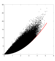
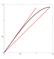
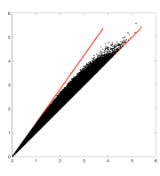
Figure 1: Illustration of Example 10. Here, we take $V:=\mathbb{R}^{2}$ and $G:=\{\pm\operatorname{id}\}\leq O(2)$. The horizontal and vertical axes represent input and output distances, respectively. (left) Draw a million pairs of vectors $x,y\in\mathbb{R}^{2}$ with standard gaussian distribution and plot the output distance $\|xx^{\top}-yy^{\top}\|_{F}$ versus the input distance $d([x],[y])$. One can show that if the input distance is $a>0$, then the output distance can take any value in $[a^{2}/\sqrt{2},\infty)$. The lower bound is depicted in red. Notably, the map $[x]\mapsto xx^{\top}$ is neither Lipschitz nor lower Lipschitz. (middle) Draw a million pairs of vectors $x,y\in\mathbb{R}^{2}$ uniformly from the unit circle and plot the output distance $\|xx^{\top}-yy^{\top}\|_{F}$ versus the input distance $d([x],[y])$. One can show that that if the input distance is $a>0$, then the output distance resides in the interval $[a,\sqrt{2}a]$. These bounds are depicted in red. Notably, the map $[x]\mapsto xx^{\top}$ is bilipschitz when restricted to $S(\mathbb{R}^{2})/G$. (right) Draw a million pairs of vectors $x,y\in\mathbb{R}^{2}$ with standard gaussian distribution and plot the output distance $\|\frac{1}{\|x\|}xx^{\top}-\frac{1}{\|y\|}yy^{\top}\|_{F}$ versus the input distance $d([x],[y])$. One can show that that if the input distance is $a>0$, then the output distance resides in the interval $[a,\sqrt{2}a]$. These bounds are depicted in red. Notably, the map $[x]\mapsto\frac{1}{\|x\|}xx^{\top}$ is bilipschitz. More generally, Theorem 13 gives that the homogeneous extension of a bilipschitz map is bilipschitz.

The above example motivates the following definition:

Definition 11.

The homogeneous extension of $f\colon S(V)//G\to S(W)$ is $f^{\star}\colon V//G\to W$ defined by $f^{\star}([cu])=cf([u])$ for $u\in S(V)$ and $c\geq 0$.

Figure 2: Illustration of homogeneous extension. See Definition 11.

See Figure 2 for an illustration. A related notion appears in Definition 3.3 of [45]. It is routine to verify that the homogeneous extension is well defined. We note that [27] considers homogeneous extensions of functions with codomain $W$ (see Definition 2 in [27]). By instead taking the codomain to be $S(W)$, the lower Lipschitz bound of $f$ quantifies the non-parallel property (see Definition 1 in [27]), which in turn produces a lower Lipschitz bound of the homogeneous extension; this is a quantitative version of Proposition 1(b) in [27]. In fact, we obtain optimal bilipschitz bounds in Theorem 13 below (cf. the upper Lipschitz bound given in Theorem 4 of [27] and the distortion bound given in Lemma 3.5 of [45].).

Lemma 12 (radial Pythagorean theorem).

For $u,v\in S(V)$ and $a,b\geq 0$, it holds that

$$d([au],[bv])^{2}=(a-b)^{2}+ab\cdot d([u],[v])^{2}.$$

Proof.

Write $d([au],[bv])^{2}=a^{2}-2ab\langle\langle[u],[v]\rangle\rangle+b^{2}$ and apply $2\langle\langle[u],[v]\rangle\rangle=2-d([u],[v])^{2}$. ∎

When $G$ is trivial, Lemma 12 reduces to the following (surprisingly unfamiliar) identity:

$$\|au-bv\|^{2}=(a-b)^{2}+ab\|u-v\|^{2}.$$

In this setting, $a$ and $b$ need not be nonnegative for the identity to hold.

In what follows, we say a group $G$ acts topologically transitively on a topological space $X$ if there exists $x\in X$ such that the orbit $G\cdot x$ is dense in $X$. For example, the group of rotations by rational multiples of $\pi$ acts topologically transitively on the unit circle. By Lemma 8, when $G$ acts by isometries on a metric space $X$, topological transitivity is equivalent to $X//G$ being a singleton set. Since bilipschitzness is ill-defined for maps on the singleton metric space, the following result isolates the topologically transitive case for completeness.

Theorem 13.

Consider any $G\leq O(V)$.

• If $G$ acts topologically transitively on $S(V)$, then for every $f\colon S(V)//G\to S(W)$, the homogeneous extension $f^{\star}\colon V//G\to W$ is an isometry.

• If $G$ does not act topologically transitively on $S(V)$, then for every $f\colon S(V)//G\to S(W)$ with optimal bilipschitz bounds $\alpha$ and $\beta$, the homogeneous extension $f^{\star}\colon V//G\to W$ has optimal bilipschitz bounds $\min\{\alpha,1\}$ and $\max\{\beta,1\}$.

Proof.

For (a), $S(V)//G$ is a singleton set, so the image of $f$ consists of a single unit vector $w\in S(W)$. Fix $u,v\in S(V)$ and $a,b\geq 0$. Then $d([u],[v])=0$, and so Lemma 12 gives

$$\|f^{\star}([au])-f^{\star}([bv])\|^{2}=\|af([u])-bf([v])\|^{2}=\|aw-bw\|^{2}=(a-b)^{2}=d([au],[bv])^{2}.$$

For (b), fix $u,v\in S(V)$ and $a,b\geq 0$. Then Lemma 12 gives

$$\|f^{\star}([au])-f^{\star}([bv])\|^{2}=\|af([u])-bf([v])\|^{2}=(a-b)^{2}+ab\|f([u])-f([v])\|^{2}.$$

Since $f$ has lower Lipschitz bound $\alpha$, we then have

$$\|f^{\star}([au])-f^{\star}([bv])\|^{2} \geq(a-b)^{2}+ab\cdot\alpha^{2}d([u],[v])^{2}$$

$$\geq\min\{\alpha,1\}^{2}\cdot\Big{(}(a-b)^{2}+ab\cdot d([u],[v])^{2}\Big{)}$$

$$=\min\{\alpha,1\}^{2}\cdot d([au],[bv])^{2},$$

where the last step applies Lemma 12. In the case where $\min\{\alpha,1\}=1$, this bound is sharp when $[u]=[v]$ and $a\neq b$, by Lemma 12. In the case where $\min\{\alpha,1\}=\alpha$, this bound is sharp when $a=b=1$ since $\alpha$ is the optimal lower Lipschitz bound for $f$ by assumption. A similar argument delivers the optimal upper Lipschitz bound. ∎

In practice, one might encounter $f$ with optimal lower Lipschitz bound $\alpha>1$, in which case the homogeneous extension $f^{\star}$ has distortion $\beta$, which is strictly larger than the distortion $\beta/\alpha$ of $f$. In this case, we can first modify $f$ by lifting outputs into an extra dimension:

Lemma 14.

Given $f\colon X\to S(W)$ with optimal bilipschitz bounds $\alpha$ and $\beta$, then for each $t\in(0,1]$, the map $f_{t}\colon X\to S(W\oplus\mathbb{R})$ defined by $f_{t}(x)=(tf(x),\sqrt{1-t^{2}})$ has optimal bilipschitz bounds $t\alpha$ and $t\beta$.

Proof.

The result follows from the fact that $\|f_{t}(x)-f_{t}(y)\|^{2}=t^{2}\|f(x)-f(y)\|^{2}$. ∎

Given $f\colon S(V)//G\to S(W)$ with optimal bilipschitz bounds $\alpha>1$ and $\beta$, then for every $t\in[\beta^{-1},\alpha^{-1}]$, the homogeneous extension $(f_{t})^{\star}$ also has distortion $\beta/\alpha$. In the case where $\beta<1$, we do not have an approach to make homogeneous extension preserve distortion. Next, we show how a generalization of the same lift can be used to convert a bounded bilipschitz map $S(V)//G\to W$ into a bilipschitz map $S(V)//G\to S(W\oplus\mathbb{R})$:

Lemma 15.

Given bounded $g\colon X\to W$ with bilipschitz bounds $\alpha$ and $\beta$, then for each $t\in(0,\|g\|_{\infty}^{-1})$, the map $g_{t}\colon X\to S(W\oplus\mathbb{R})$ defined by $g_{t}(x)=(tg(x),\sqrt{1-\|tg(x)\|^{2}})$ has (possibly suboptimal) bilipschitz bounds $t\alpha$ and $(1-t^{2}\|g\|_{\infty}^{2})^{-1/2}\cdot t\beta$.

Proof.

The lower Lipschitz bound follows from the fact that $\|g_{t}(x)-g_{t}(y)\|\geq t\|g(x)-g(y)\|$. For the upper Lipschitz bound, put $r:=\|g\|_{\infty}$ and consider the map $h_{t}\colon[0,tr]\to\mathbb{R}$ defined by $h_{t}(u)=\sqrt{1-u^{2}}$. The derivative of $h_{t}$ reveals that its optimal upper Lipschitz bound is $c_{t}:=(1-t^{2}r^{2})^{-1/2}\cdot tr$. We apply this bound and the reverse triangle inequality to obtain

$$\|g_{t}(x)-g_{t}(y)\|^{2} =t^{2}\|g(x)-g(y)\|^{2}+\big{|}h_{t}(\|tg(x)\|)-h_{t}(\|tg(y)\|)\big{|}^{2}$$

$$\leq t^{2}\|g(x)-g(y)\|^{2}+c_{t}^{2}\cdot\big{|}\|tg(x)\|-\|tg(y)\|\big{|}^{2}\leq t^{2}(1+c_{t}^{2})\|g(x)-g(y)\|^{2},$$

and the result follows. ∎

Notably, Lemma 15 produces a map with near identical distortion when $t$ is small, but taking $t$ too small will send the upper Lipschitz bound below $1$, in which case homogeneous extension will increase the distortion.

In what follows, we describe a few examples of bilipschitz maps over $S(V)//G$ that can be homogeneously extended to bilipschitz maps over $V//G$ by Theorem 13(b).

Example 16 (cf. Example 10).

Fix a nontrivial real Hilbert space $V$, take $G:=\{\pm\operatorname{id}\}\leq O(V)$, and consider $f\colon S(V)/G\to S(V^{\otimes 2})$ defined by $f([x])=x\otimes x$. If $V$ has dimension $1$, then $G$ acts transitively on $S(V)$, and so Theorem 13(a) applies. Otherwise, for each $x,y\in S(V)$ with $[x]\neq[y]$, we have

$$d([x],[y])^{2}=\min\{\|x-y\|^{2},\|x+y\|^{2}\}=2-2|\langle x,y\rangle|,$$

$$\|f([x])-f([y])\|^{2}=2-2\langle x\otimes x,y\otimes y\rangle=2-2\langle x,y\rangle^{2},$$

and so taking $t:=|\langle x,y\rangle|$ gives

$$\frac{\|f([x])-f([y])\|}{d([x],[y])}=\sqrt{\frac{1-t^{2}}{1-t}}=\sqrt{1+t}.$$

Since $t$ takes values in $[0,1)$, it follows that $f$ has optimal bilipschitz bounds $1$ and $\sqrt{2}$. By Theorem 13(b), the homogeneous extension

$$f^{\star}(x)=\left\{\begin{array}[]{cl}\displaystyle\frac{x\otimes x}{\|x\|}&\text{if $x\neq 0$}\vspace{0.1in}\\ 0&\text{otherwise}\end{array}\right.$$

has the same optimal bilipschitz bounds. By Corollary 36, this is the minimum possible distortion for a Euclidean embedding of $V/G$. By contrast, in the case where $V=\ell^{2}$, max filtering approaches fail to deliver bilipschitz invariants [25, 1].

Example 17.

Fix a nontrivial complex Hilbert space $V$, take $G:=\{\omega\cdot\operatorname{id}:|\omega|=1\}\leq U(V)$, and consider $f\colon S(V)/G\to S(V\otimes V^{*})$ defined by $f([x])=x\otimes\langle x,\cdot\rangle$. If $V$ has dimension $1$, then $G$ acts transitively on $S(V)$, and so Theorem 13(a) applies. Otherwise, following the argument in Example 16, then for any $x,y\in S(V)$, we have

$$d([x],[y])^{2}=2-2|\langle x,y\rangle|,\qquad\|f([x])-f([y])\|^{2}=2-2|\langle x,y\rangle|^{2},$$

and $f$ has optimal bilipschitz bounds $1$ and $\sqrt{2}$. By Theorem 13(b), the homogeneous extension $f^{\star}$ has the same optimal bilipschitz bounds. By Corollary 37, this is the minimum distortion for a Euclidean embedding of $V/G$.

Example 18.

Fix $V:=\mathbb{C}$, take $G:=\langle e^{2\pi i/r}\rangle\leq U(1)$ for some $r\in\mathbb{N}$, and consider $f\colon S(V)/G\to S(V)$ defined by $f([x])=x^{r}$. Then for every $x,y\in S(V)$, we have

$$d([x],[y])^{2}=2-2\max_{g\in G}\operatorname{Re}(gx\overline{y}),\qquad\|f([x])-f([y])\|^{2}=2-2\operatorname{Re}((x\overline{y})^{r}).$$

When $[x]\neq[y]$, we take $h\in G$ such that $hx\overline{y}=e^{2\pi it}$ for some $t\in[-\frac{1}{2r},\frac{1}{2r})\setminus\{0\}$. Then

$$\frac{\|f([x])-f([y])\|}{d([x],[y])}=\sqrt{\frac{1-\operatorname{Re}((x\overline{y})^{r})}{1-\displaystyle\max_{g\in G}\operatorname{Re}(gx\overline{y})}}=\sqrt{\frac{1-\operatorname{Re}((hx\overline{y})^{r})}{1-\displaystyle\max_{g\in G}\operatorname{Re}(ghx\overline{y})}}=\frac{\sin(\pi rt)}{\sin(\pi t)}=:g(t).$$

We note that $g$ is decreasing on $(0,\frac{1}{2r})$ since $g^{\prime}(t)<0$ precisely when $\frac{\tan(\pi t)}{\pi t}<\frac{\tan(\pi rt)}{\pi rt}$, while $\frac{d}{dx}(\frac{\tan(x)}{x})>0$ for $x\in(0,\frac{\pi}{2})$ since $\sin(x)\cos(x)<x$. Since $g$ is even, evaluating at $t=\frac{1}{2r}$ and taking the limit $t\to 0$ gives the optimal bilipschitz bounds, namely, $\csc(\frac{\pi}{2r})$ and $r$. Notably, $\csc(\frac{\pi}{2r})>1$ when $r>1$, so one should lift as in Lemma 14 before taking the homogeneous extension in order to preserve the distortion $r\sin(\frac{\pi}{2r})\in[1,\frac{\pi}{2})$. By Corollary 38, this is the minimum distortion for a Euclidean embedding of $V/G$.

5 Non-differentiability of bilipschitz invariants

We motivate this section with an example:

Example 19.

By Proposition 9, max filtering produces bilipschitz invariants modulo finite groups of $O(d)$. However, these invariants fail to be differentiable. Indeed, $x\mapsto\langle\langle[z],[x]\rangle\rangle$ is non-differentiable precisely at the boundaries of the Voronoi diagram of the orbit $G\cdot z$. For an explicit example, take $V:=\mathbb{R}^{2}$, templates $z_{1}:=(1,1)$, $z_{2}:=(1,2)$, and $z_{3}:=(3,1)$, and given $G\leq O(2)$, consider the max filtering invariant

$$f\colon x\mapsto\Big{(}~{}\langle\langle[z_{1}],[x]\rangle\rangle,~{}\langle\langle[z_{2}],[x]\rangle\rangle,~{}\langle\langle[z_{3}],[x]\rangle\rangle~{}\Big{)}.$$

We consider two cases: when $G$ consists of rotations by multiples of $2\pi/3$, and when $G$ is the dihedral group of order $6$. See Figure 3 for an illustration. The points at which $f$ is not differentiable form rays emanating from the origin. Later in this section, we show that every point with a nontrivial stabilizer in $G$ (i.e., every non-principal point) is necessarily a point of non-differentiability in any bilipschitz invariant; see Theorem 21(b). In both parts of Figure 3 (and in fact, whenever $G$ is nontrivial), the origin is one such non-principal point. In the example on the left, this is the only non-principal point, whereas on the right, every non-differentiable point is a non-principal point. In what follows, we show how bilipschitzness requires such non-differentiability of max filtering invariants.

Figure 3: Illustration of Example 19. Max filtering invariants are piecewise linear. In this example, the orbits of the templates $z_{1},z_{2},z_{3}\in\mathbb{R}^{2}$ determine points of non-differentiability (namely, the boundaries of their Voronoi cells) in the resulting max filtering invariant. On the left, the group $G\leq O(2)$ consists of rotations by multiples of $2\pi/3$, while on the right, $G$ is the dihedral group of order $6$. Considering Theorem 21(b), the non-differentiability of max filtering is an artifact of its bilipschitzness.

Recall that a function $f\colon V\to W$ is Fréchet differentiable at $x\in V$ if there exists a bounded linear map $A\colon V\to W$ such that

$$\lim_{h\to 0}\frac{\|f(x+h)-f(x)-Ah\|}{\|h\|}=0,$$

in which case we say $A$ is the Fréchet derivative at $x$, which we denote by $Df(x):=A$; see [32] for more information. If $V$ and $W$ are Euclidean, then the matrix representation of $Df(x)$ is the Jacobian of $f$ at $x$.

Lemma 20.

Suppose $f\colon V\to W$ is $G$-invariant and Fréchet differentiable at $x\in V$. Then for each $g\in G$, it holds that $f$ is Fréchet differentiable at $gx$ with $Df(gx)=Df(x)\circ g^{-1}$.

Proof.

By $G$-invariance, we have $f(gx)=f(x)$ and $f(gx+h)=f(x+g^{-1}h)$, and so

$$\lim_{h\to 0}\frac{\|f(gx+h)-f(gx)-(Df(x)\circ g^{-1})h\|}{\|h\|}=\lim_{h\to 0}\frac{\|f(x+g^{-1}h)-f(x)-Df(x)(g^{-1}h)\|}{\|g^{-1}h\|}.$$

Change variables $g^{-1}h\mapsto h$ and apply Fréchet differentiability at $x$ to obtain the result. ∎

Theorem 21.

Suppose $x\in V$ is fixed by some nonidentity member of $G$, and consider any $G$-invariant map $f\colon V\to W$ that is Fréchet differentiable at $x$. Then the following hold.

• There exists a unit vector $v\in V$ orthogonal to $x$ such that $Df(x)v=0$.

• If $G$ is finite or $x=0$, then $f^{\downarrow}\colon V//G\to W$ is not lower Lipschitz.

• If $G$ is finite and $x\in S(V)$, then the restriction $f^{\downarrow}|_{S(V)/G}$ is not lower Lipschitz.

In words, a bilipschitz invariant cannot be differentiable at any point with a nontrivial stabilizer. In particular, if $G$ is nontrivial, no bilipschitz invariant is differentiable at $0$. For each example in Section 4, $G$ acts freely on $V\setminus\{0\}$, and so we can get away with $0$ being the only point at which $f$ is not differentiable.

Proof of Theorem 21.

For (a), fix a nontrivial $g\in G$ with $gx=x$. Since $\operatorname{ker}(g-\operatorname{id})$ is a closed and proper subspace of $V$, there is a unit vector $v$ in $\operatorname{ker}(g-\operatorname{id})^{\perp}$. Notably, $v$ is orthogonal to $x\in\operatorname{ker}(g-\operatorname{id})$. It remains to show $Df(x)v=0$. By Lemma 20, $Df(x)=Df(gx)=Df(x)\circ g^{-1}$, and so $Df(x)^{*}=g\circ Df(x)^{*}$. Thus, $g$ fixes every element of $\operatorname{im}Df(x)^{*}$ so that $\operatorname{im}Df(x)^{*}\leq\operatorname{ker}(g-\operatorname{id})$. Then $v\in\operatorname{ker}(g-\operatorname{id})^{\perp}\leq(\operatorname{im}Df(x)^{*})^{\perp}=\operatorname{ker}Df(x)$.

For (b), take $v\in V$ from (a). Since $G$ is finite or $x=0$, either the members of $[x]$ have some minimum pairwise distance $\delta>0$, or $[x]$ is a singleton set and we may take $\delta:=\infty$ in what follows. For every $t\in\mathbb{R}$ such that $|t|<\delta/2$, it holds that $d([x+tv],[x])=|t|$, since every $y\in[x]\setminus\{x\}$ satisfies $\|(x+tv)-y\|\geq||t|-\|y-x\||>|t|$. The definition of the Fréchet derivative then implies

$$\liminf_{t\to 0}\frac{\|f^{\downarrow}([x+tv])-f^{\downarrow}([x])\|}{d([x+tv],[x])}=\liminf_{t\to 0}\frac{\|f(x+tv)-f(x)-Df(x)tv\|}{|t|}=0.$$

Thus, $f^{\downarrow}$ is not lower Lipschitz.

For (c), we argue as in (b) with a different perturbation of $x$. Take $v$ from (a) and put $h(t):=x\cos(t)+v\sin(t)-x$ so that $x+h(t)\in S(V)$ for all $t$. An argument like above shows $d([x+h(t)],[x])=\|h(t)\|$ when $|t|$ is sufficiently small. We apply the triangle inequality, the definition of the Fréchet derivative, and the fact that $Df(x)v=0$ to get

$$\liminf_{t\to 0}\frac{\|f^{\downarrow}([x+h(t)])-f^{\downarrow}([x])\|}{d([x+h(t)],[x])}=\liminf_{t\to 0}\frac{\|f(x+h(t))-f(x)\|}{\|h(t)\|}$$

$$\leq\liminf_{t\to 0}\frac{\|f(x+h(t))-f(x)-Df(x)h(t)\|+\|Df(x)(h(t)-tv)\|+\|Df(x)tv\|}{\|h(t)\|}$$

$$=\liminf_{t\to 0}\frac{\|Df(x)(h(t)-tv)\|}{\|h(t)\|}\leq\|Df(x)\|\cdot\liminf_{t\to 0}\frac{\|h(t)-tv\|}{\|h(t)\|}.$$

Considering $\|h(t)-tv\|^{2}=(\cos t-1)^{2}+(\sin t-t)^{2}$ and $\|h(t)\|^{2}=(\cos t-1)^{2}+\sin^{2}t$, the $\liminf$ above is zero, and so $f^{\downarrow}|_{S(V)/G}$ is not lower Lipschitz. ∎

Example 22.

As an application, consider the problem of multi-reference alignment [15]. Here, $G$ is the group of cyclic permutations, and the task is to estimate an unknown $[x]\in\mathbb{C}^{d}/G$ given data of the form $\{g_{i}x+z_{i}\}_{i=1}^{n}$, where the $g_{i}$’s are drawn uniformly from $G$ and the $z_{i}$’s are independent complex gaussian vectors with large variance. If $G$ were trivial, then one could estimate $x$ with the sample average. Since $G$ is nontrivial, we are inclined to “average out the noise” in an invariant domain.

One popular invariant is the bispectrum $B\colon\mathbb{C}^{d}\to\mathbb{C}^{d^{2}}$ defined by

$$B(x)_{k\ell}=\hat{x}(k)\cdot\overline{\hat{x}(\ell)}\cdot\hat{x}(\ell-k),$$

where $\hat{x}$ denotes the discrete Fourier transform of $x$, and $\ell-k$ is interpreted modulo $d$. The approach in [15] performs multi-reference alignment by first using the data $\{g_{i}x+z_{i}\}_{i=1}^{n}$ to find an estimate $y$ of $B(x)$, and then using $y$ to estimate $[x]$. For the second step, they construct a function $\psi\colon(\mathbb{C}^{\times})^{d^{2}}\to\mathbb{C}^{d}/G$ such that $\psi(B^{\downarrow}([x]))=[x]$ whenever $\hat{x}$ is everywhere nonzero, and they show that $\psi$ is locally Lipschitz.

In what follows, we show that $\psi$ is not Lipschitz as a consequence of Theorem 21(b). Suppose otherwise that $\psi$ is $\beta$-Lipschitz, and let $U$ denote the vectors in $\mathbb{C}^{d}$ with everywhere nonzero discrete Fourier transform. Since $U$ is dense in $\mathbb{C}^{d}$ and $B$ (and hence $B^{\downarrow}$) is continuous, we have

$$\inf_{\begin{subarray}{c}x,y\in\mathbb{C}^{d}\\ {[x]\neq[y]}\end{subarray}}\frac{\|B^{\downarrow}([x])-B^{\downarrow}([y])\|}{d([x],[y])}=\inf_{\begin{subarray}{c}x,y\in U\\ {[x]\neq[y]}\end{subarray}}\frac{\|B^{\downarrow}([x])-B^{\downarrow}([y])\|}{d([x],[y])}=\inf_{\begin{subarray}{c}x,y\in U\\ {[x]\neq[y]}\end{subarray}}\frac{\|B^{\downarrow}([x])-B^{\downarrow}([y])\|}{d(\psi(B^{\downarrow}([x])),\psi(B^{\downarrow}([y])))}\geq\frac{1}{\beta},$$

i.e., $B^{\downarrow}$ is $1/\beta$-lower Lipschitz. Since $G$ fixes the constant functions and $B$ is differentiable as a map between real Hilbert spaces, this contradicts Theorem 21(b). In general, a left inverse to a translation-invariant map $f$ cannot be Lipschitz unless $f$ is not differentiable at the constant functions (and at any other nontrivially periodic function). Such non-differentiability is afforded by max filtering, which in turn delivers bilipschitz invariants [28].

6 Bilipschitz polynomial invariants

Classical invariant theory is concerned with polynomial maps, thanks in part to the following well-known result.

Proposition 23.

For each finite $G\leq GL(d)$, there exists an injective polynomial map $\mathbb{R}^{d}/G\to\mathbb{R}^{n}$ for some $n\in\mathbb{N}$.

Proof.

First, we observe that every pair of distinct $G$-orbits $[x],[y]\in\mathbb{R}^{d}/G$ is necessarily separated by some $G$-invariant polynomial function $f\colon\mathbb{R}^{d}\to\mathbb{R}$. For example, applying the Reynolds operator $h\mapsto\frac{1}{|G|}\sum_{g\in G}(g\cdot h)$ to the map $h\colon z\mapsto\prod_{g\in G}\|z-gx\|^{2}$ gives such an $f$, since then $f(z)\geq 0$ with equality precisely when $z\in[x]$. Next, Hilbert [54] established that the algebra of $G$-invariant polynomials with complex coefficients is generated by finitely many polynomials $\{h_{i}(x)\}_{i=1}^{k}$. Thus, every pair of distinct $G$-orbits in $\mathbb{R}^{d}$ is necessarily separated by some $h_{i}\colon\mathbb{R}^{d}\to\mathbb{C}$. Defining $h\colon\mathbb{R}^{d}\to\mathbb{C}^{k}\cong\mathbb{R}^{2k}$ by $h(x):=(h_{1}(x),\ldots,h_{k}(x))$, then $h^{\downarrow}$ is the desired injection. ∎

In this section, we evaluate polynomial maps in terms of bilipschitzness.

Lemma 24.

Suppose $G\leq O(d)$ is nontrivial and $f\colon\mathbb{R}^{d}\to\mathbb{R}^{n}$ is a $G$-invariant polynomial. Then $f^{\downarrow}\colon\mathbb{R}^{d}//G\to\mathbb{R}^{n}$ is not lower Lipschitz. Furthermore, $f^{\downarrow}$ is upper Lipschitz only if $f$ is affine linear, in which case $f^{\downarrow}$ is not injective.

Proof.

Since the origin has a nontrivial stabilizer and $f$ is differentiable at the origin, Theorem 21 gives that $f^{\downarrow}$ is not lower Lipschitz.

Next, suppose $f$ is not affine linear. We will show that $f^{\downarrow}$ is not upper Lipschitz. Select a coordinate function $f_{i}(x)$ of degree $k\geq 2$, and let $g(x)$ denote the homogeneous component of $f_{i}(x)$ of degree $k$. Since $g(x)$ is nonzero, there exists $v\in\mathbb{R}^{d}$ such that $g(v)\neq 0$. Note that $g(0)=0$ by homogeneity, and so $v\neq 0$. Then $g(tv)=t^{k}g(v)$, and so $f_{i}(tv)=t^{k}g(v)+O(t^{k-1})$ for large $t$. Thus, $\|f^{\downarrow}([tv])-f^{\downarrow}([0])\|\geq|f_{i}(tv)-f_{i}(0)|=|t^{k}g(v)+O(t^{k-1})|=t^{k}|g(v)|+O(t^{k-1})$ for large $t$. Since $d([tv],[0])=|t|\|v\|$, it follows that $f^{\downarrow}$ is not upper Lipschitz.

Finally, suppose $f$ is affine linear and write $f(x)=Ax+b$. Since $G$ is nontrivial, there exists $g\in G$ and $y\in\mathbb{R}^{d}$ such that $z:=gy\neq y$. Then $f(y)=f(z)$, meaning $Ay+b=Az+b$, and so $A(y-z)=0$. It follows that $f^{\downarrow}([y-z])=f^{\downarrow}([0])$, i.e., $f^{\downarrow}$ is not injective. ∎

While we cannot expect polynomial invariants to be bilipschitz, there is some hope of applying ideas from Section 4 to obtain bilipschitz maps from polynomial invariants by homogeneous extension. In fact, all of the examples from Section 4 were obtained in this way. Considering Lemma 15, it suffices to seek $G$-invariant polynomial maps $f\colon\mathbb{R}^{d}\to\mathbb{R}^{n}$ for which $f^{\downarrow}|_{S(\mathbb{R}^{d})//G}$ is bilipschitz. By Theorem 21(c), this is not possible when $G$ is finite unless it acts freely on $S(\mathbb{R}^{d})$. (Indeed, for each example in Section 4, $G$ acts freely.) This is a strong condition, and it implies that every abelian subgroup of $G$ is cyclic; see Theorems 5.3.1 and 5.3.2 in [91]. Nevertheless, nonabelian examples exist, and furthermore, they have been classified; see Chapter 6 of [91]. Interestingly, every one of these examples admits a polynomial $f\colon\mathbb{R}^{d}\to\mathbb{R}^{n}$ for which $f^{\downarrow}|_{S(\mathbb{R}^{d})/G}$ is bilipschitz:

Theorem 25.

For finite $G\leq O(d)$, the following are equivalent:

• $G$ acts freely on $S(\mathbb{R}^{d})$.

• There exists a bilipschitz polynomial map $S(\mathbb{R}^{d})/G\to\mathbb{R}^{n}$ for some $n\in\mathbb{N}$.

• There exists a bilipschitz polynomial map $S(\mathbb{R}^{d})/G\to\mathbb{R}^{2d-1}$.

If $G\leq O(d)$ is finite and acts freely on $S(\mathbb{R}^{d})$, then one may combine Theorem 25(c) with Lemma 15 and Theorem 13(b) to obtain a bilipschitz map $\mathbb{R}^{d}/G\to\mathbb{R}^{2d}$. By comparision, max filtering delivers injective maps $\mathbb{R}^{d}/G\to\mathbb{R}^{2d}$, and while these maps are conjectured to be bilipschitz, this is currently only known for certain choices of $G$ [28, 69]. (Max filtering is known to provide bilipschitz invariants $\mathbb{R}^{d}/G\to\mathbb{R}^{n}$ for large $n$.) We will prove Theorem 25 with the help of a few (essentially known) propositions.

Proposition 26.

Given distinct $u_{1},\ldots,u_{n}\in\mathbb{R}^{d}$ and not necessarily distinct $v_{1},\ldots,v_{n}\in\mathbb{R}^{d}$, there exists a polynomial function $p\colon\mathbb{R}^{d}\to\mathbb{R}$ such that $\nabla p(u_{i})=v_{i}$ for every $i\in\{1,\ldots,n\}$.

Proof.

First, we consider the special case in which the coordinates $(u_{1})_{k},\ldots,(u_{n})_{k}$ are distinct for each $k\in\{1,\ldots,d\}$. For this case, we construct $p\colon\mathbb{R}^{d}\to\mathbb{R}$ of the form

$$p(x_{1},\ldots,x_{d})=\sum_{k=1}^{d}p_{k}(x_{k}),$$ (2)

where each $p_{k}$ is a polynomial in one variable. Then for each $k\in\{1,\ldots,d\}$, we seek a polynomial $q_{k}:=p_{k}^{\prime}$ that satisfies

$$q_{k}((u_{i})_{k})=\frac{\partial p}{\partial x_{k}}(u_{i})=(v_{i})_{k}$$

for all $i\in\{1,\ldots,n\}$. This can be accomplished by Lagrange interpolation, and we integrate to get $p_{k}$, and then (2) gives the desired polynomial.

Next, we generalize the above argument to treat the general case. To do so, we select an invertible matrix $A\in\mathbb{R}^{d\times d}$ in which a way that the coordinates $(Au_{1})_{k},\ldots,(Au_{n})_{k}$ are distinct for each $k\in\{1,\ldots,d\}$. Equivalently, $A\in\mathbb{R}^{d\times d}$ satisfies $\operatorname{det}(A)\neq 0$ and $e_{k}^{\top}A(u_{i}-u_{j})\neq 0$ for every $k\in\{1,\ldots,d\}$ and every $i,j\in\{1,\ldots,n\}$ with $i\neq j$. That is, it suffices for $A$ to be generic in the sense that it does not reside in the zero set of a nonzero polynomial. (In particular, such an $A$ necessarily exists.) Consider $\overline{u}_{i}:=Au_{i}$ and $\overline{v}_{i}:=(A^{\top})^{-1}v_{i}$ for all $i\in\{1,\ldots,n\}$. Since the coordinates $(u_{1})_{k},\ldots,(u_{n})_{k}$ are distinct for each $k\in\{1,\ldots,d\}$, our treatment of the previous case delivers a polynomial function $\overline{p}$ such that $\nabla\overline{p}(\overline{u}_{i})=\overline{v}_{i}$ for all $i\in\{1,\ldots,n\}$. Denoting $L\colon x\mapsto Ax$ and $p:=\overline{p}\circ L$, then since the Jacobian of $\overline{p}$ at $x$ is $\nabla\overline{p}(x)^{\top}$, the chain rule gives

$$v_{i}^{\top}=\overline{v}_{i}^{\top}A=\nabla\overline{p}(\overline{u}_{i})^{\top}A=\nabla(\overline{p}\circ L)(u_{i})^{\top}=\nabla p(u_{i})^{\top},$$

that is, $\nabla p(u_{i})=v_{i}$ for every $i\in\{1,\ldots,n\}$, as desired. ∎

Proposition 27.

Given a finite group $G$ acting freely on a smooth manifold $M$ and a $G$-invariant immersion $g\colon M\to\mathbb{R}^{n}$, then $M/G$ is a smooth manifold with the same dimension as $M$ and the corresponding map $g^{\downarrow}\colon M/G\to\mathbb{R}^{n}$ is an immersion.

Proof.

Consider $\pi\colon M\to M/G$ defined by $\pi(x)=[x]$. Since $G$ is finite and acts freely, $M/G$ is a topological manifold with the same dimension as $M$, and with a unique smooth structure for which $\pi$ is a smooth submersion (see Theorem 21.10 in [63]). Apply the chain rule to $g=g^{\downarrow}\circ\pi$ at an arbitrary point $x\in M$:

$$Dg(x)=Dg^{\downarrow}([x])\circ D\pi(x).$$

Since $g$ is an immersion, $Dg(x)$ is injective. Since $\pi$ is a submersion, $D\pi(x)$ is a surjective linear map between vector spaces of the same dimension, i.e., a bijection. It follows that $Dg^{\downarrow}([x])$ is injective, i.e., $g^{\downarrow}$ is an immersion. ∎

Proposition 28.

For smooth Riemannian manifolds $X$ and $Y$ with $X$ compact, every smooth embedding $X\to Y$ is bilipschitz.

Proof.

We present an argument from Moishe Kohan [60]. Fix a smooth embedding $f\colon X\to Y$. To prove upper Lipschitz, take any $p,q\in X$ and let $c\colon[0,d_{X}(p,q)]\to X$ denote the unit-speed parameterization of a shortest path from $p$ to $q$. Then

$$d_{Y}(f(p),f(q)) =\int_{0}^{d_{X}(p,q)}\|(f\circ c)^{\prime}(t)\|dt=\int_{0}^{d_{X}(p,q)}\|(Df)(c(t))c^{\prime}(t)\|dt$$

$$\leq\sup_{x\in X}\|(Df)(x)\|\cdot\int_{0}^{d_{X}(p,q)}\|c^{\prime}(t)\|dt=\sup_{x\in X}\|(Df)(x)\|\cdot d_{X}(p,q).$$

Furthermore, $\sup_{x\in X}\|(Df)(x)\|<\infty$ by compactness.

Next, we show that $f$ is locally lower Lipschitz in the sense that there exists $\alpha,\epsilon>0$ such that $d_{Y}(f(p),f(q))\geq\alpha d_{X}(p,q)$ whenever $d_{X}(p,q)<\epsilon$. First, $Z:=\operatorname{im}(f)$ is a compact submanifold of $Y$, and so it has a normal injectivity radius $r>0$. That is, letting $B_{r}\nu_{Z}$ denote the members of the normal bundle $\nu_{Z}$ of $Z$ in $Y$ with norm smaller than $r$, then the restriction of the normal exponential map $\operatorname{exp}_{Z}\colon\nu_{Z}\to Y$ to $B_{r}\nu_{Z}$ is a diffeomorphism onto its image $N\subseteq Y$, which in turn is an open tubular neighborhood of $Z$. Invert this diffeomorphism and project onto $Z$ to obtain a smooth retraction $p\colon N\to Z$. Applying $\operatorname{exp}_{Z}$ to the closure of $B_{r/2}\nu_{Z}$ gives a compact submanifold with boundary $K\subseteq N$, and so the previous argument gives that $p|_{K}$ is Lipschitz, even if we take $Z$ to have the Riemannian metric from $X$. Since $d_{Y}(p,q)=d_{K}(p,q)$ whenever $d_{Y}(p,q)$ is sufficiently small, and since $f$ is Lipschitz, it follows that $f$ is $\epsilon$-locally $\alpha$-lower Lipschitz for some $\alpha,\epsilon>0$.

Finally, consider the set $C$ of $(p,q)\in X^{2}$ for which $d_{X}(p,q)\geq\epsilon$. Then compactness gives

$$R:=\sup_{(p,q)\in C}\frac{d_{X}(p,q)}{d_{Y}(f(p),f(q))}<\infty.$$

Since $f$ is $\epsilon$-locally $\alpha$-lower Lipschitz, it follows that $f$ is $\min\{\alpha,1/R\}$-lower Lipschitz. ∎

Proposition 29.

Given a $k$-dimensional semialgebraic submanifold $M$ of $\mathbb{R}^{n}$ and $m>2k$, then for a generic linear map $L\colon\mathbb{R}^{n}\to\mathbb{R}^{m}$, the restriction $L|_{M}$ is an embedding.

Proof.

First, we note that $L|_{M}$ is not injective precisely when there exist $x,y\in M$ with $x\neq y$ such that $L(x-y)=0$. Similarly, $L|_{M}$ is not an immersion precisely when there exists $x\in M$ and a nonzero $v\in T_{x}M$ such that $Lv=0$. Letting $W$ denote the set of all such $x-y$ and $v$, then $L|_{M}$ is not an embedding precisely when there exists $w\in W$ such that $Lw=0$. Consider the set $P$ of $(L,w)$ for which $Lw=0$ and $w\in W$. Then $L|_{M}$ is an embedding precisely when $L$ does not reside in the projection $\pi_{L}(P)$. Lemma 1.10 in [43] gives

$$\operatorname{dim}\pi_{L}(P)\leq\operatorname{dim}P\leq\operatorname{dim}W+\sup_{w\in W}\operatorname{dim}\{L:(L,w)\in P\}.$$

Meanwhile, $\operatorname{dim}W=2k$ and $\operatorname{dim}\{L:Lw=0\}=m(n-1)$ for every $w\neq 0$. Thus, $\operatorname{dim}\pi_{L}(P)\leq 2k+m(n-1)$, which is strictly less than $mn$ when $m>2k$. It follows that a generic choice of $L$ does not reside in $\pi_{L}(P)$. ∎

Proof of Theorem 25.

First, (c)$\Rightarrow$(a) follows from Theorem 21(c).

For (a)$\Rightarrow$(b), we first claim that for every $u\in S(\mathbb{R}^{d})$, there exists a $G$-invariant polynomial map $p_{u}\colon\mathbb{R}^{d}\to\mathbb{R}^{d}$ such that $Dp_{u}(u)$ is invertible. To see this, for each $i\in\{1,\ldots,d\}$, take any polynomial $q_{u,i}\colon\mathbb{R}^{d}\to\mathbb{R}$ such that $\nabla q_{u,i}(gu)=ge_{i}$ for all $g\in G$. Such a polynomial exists by Proposition 26; indeed, $\{gu\}_{g\in G}$ are distinct since $G$ acts freely on $S(\mathbb{R}^{d})$ by assumption. Let $\overline{q}_{u,i}$ denote the $G$-invariant polynomial map obtained by applying the Reynolds operator to $q_{u,i}$. Then

$$\nabla\overline{q}_{u,i}(x)^{\top}=\frac{1}{|G|}\sum_{g\in G}\nabla(q_{u,i}\circ g)(x)^{\top}=\frac{1}{|G|}\sum_{g\in G}\nabla q_{u,i}(gx)^{\top}g.$$

Evaluating at $x=u$ then gives

$$\nabla\overline{q}_{u,i}(u)^{\top}=\frac{1}{|G|}\sum_{g\in G}\nabla q_{u,i}(gu)^{\top}g=\frac{1}{|G|}\sum_{g\in G}(ge_{i})^{\top}g=e_{i}^{\top}.$$

Then taking $p_{u}(x):=(\overline{q}_{u,1}(x),\ldots,\overline{q}_{u,d}(x))$ gives $Dp_{u}(u)=\operatorname{id}$, as desired.

Next, by the continuity of $x\mapsto\operatorname{det}(Dp_{u}(x))$, we have that $Dp_{u}(x)$ is invertible on an open neighborhood $N_{u}$ of $u$. By compactness, the open cover $\{N_{u}\}_{u\in S(\mathbb{R}^{d})}$ of $S(\mathbb{R}^{d})$ has a finite subcover $\{N_{u}\}_{u\in F}$. Then the polynomial map $r_{1}\colon x\mapsto\{p_{u}(x)\}_{u\in F}$ has the property that $Dr_{1}(x)$ is injective for every $x\in S(\mathbb{R}^{d})$. Next, let $r_{2}$ denote any polynomial $G$-invariant map that separates $G$-orbits as in Proposition 23. The polynomial map $r\colon S(\mathbb{R}^{d})\to\mathbb{R}^{n}$ defined by $r(x)=(r_{1}(x),r_{2}(x))$ is an immersion due to the $r_{1}$ component, and so Proposition 27 gives that $r^{\downarrow}$ is an immersion of $S(\mathbb{R}^{d})/G$. Furthermore, the $r_{2}$ component ensures that $r^{\downarrow}$ is injective. As such, $r^{\downarrow}$ is an embedding. Finally, the fact that $r^{\downarrow}$ is bilipschitz follows from Proposition 28. Specifically, to use this result, we note that the Euclidean metric on $S(\mathbb{R}^{d})$ is equivalent to the standard Riemannian metric, and so the quotient Euclidean metric on $S(\mathbb{R}^{d})/G$ is equivalent to the quotient Riemannian metric, which in turn is a Riemannian metric on $S(\mathbb{R}^{d})/G$ since $G\leq O(d)$.

Finally, for (b)$\Rightarrow$(c), we have a bilipschitz polynomial map $r^{\downarrow}\colon S(\mathbb{R}^{d})/G\to\mathbb{R}^{n}$. The lower Lipschitz bound ensures that $r^{\downarrow}$ is an embedding. As such, $M:=\operatorname{im}(r^{\downarrow})$ is a compact submanifold of $\mathbb{R}^{n}$ of dimension $d-1$. Furthermore, $M$ is the image of the semialgebraic set $S(\mathbb{R}^{d})$ under a polynomial map, and so it is semialgebraic. By Proposition 29, $L|_{M}$ is an embedding for a generic linear map $L\colon\mathbb{R}^{n}\to\mathbb{R}^{2d-1}$, in which case $L\circ r^{\downarrow}$ is the desired map. (Indeed, bilipschitzness follows from Proposition 28 as before.) ∎

While our proof of (a)$\Rightarrow$(b) in Theorem 25 was not constructive, the following result provides a construction in the special case where $G$ is abelian. Considering $G\leq O(d)\leq U(d)$, we may focus on the complex case without loss of generality. Then the spectral theorem affords $\mathbb{C}^{d}$ with an orthonormal basis that simultaneously diagonalizes every element of $G$, as in the hypotheses below.

Theorem 30.

Given a finite abelian $G\leq U(d)$, choose any orthonormal basis $\{u_{i}\}_{i=1}^{d}$ of $\mathbb{C}^{d}$ for which there exists characters $\{\chi_{i}\}_{i=1}^{d}$ of $G$ such that $gu_{i}=\chi_{i}(g)u_{i}$ for all $g\in G$ and $i\in\{1,\ldots,d\}$. The following are equivalent:

• $G$ acts freely on $S(\mathbb{C}^{d})$.

• For each $i\in\{1,\ldots,d\}$, the character $\chi_{i}$ is an isomorphism of $G$ onto its image.

• For each $i,j\in\{1,\ldots,d\}$, there exists a smallest integer $m_{ij}\geq 0$ for which $\chi_{i}\chi_{j}^{m_{ij}}=1$.

Furthermore, when (c) holds, the polynomial map $f\colon\mathbb{C}^{d}\to\mathbb{C}^{d\times d}$ defined by

$$f(x)=\{\langle u_{i},x\rangle\langle u_{j},x\rangle^{m_{ij}}\}_{i,j=1}^{d}$$

is $G$-invariant and $f^{\downarrow}|_{S(\mathbb{C}^{d})/G}$ is bilipschitz.

Notably, (the proof of) Proposition 5.2.1 in [42] establishes that the related map

$$p(x)=\{\langle u_{i},x\rangle\langle u_{j},x\rangle^{m_{ij}}\}_{i\leq j}$$

is $G$-invariant and $p^{\downarrow}$ is injective. Later, [27] established that while $p^{\downarrow}|_{S(\mathbb{C}^{d})/G}$ is Lipschitz, when $d\geq 3$ and $|G|\geq 3$, this function is not lower Lipschitz. With this context, Theorem 30 can be interpreted as making the injective map $p^{\downarrow}|_{S(\mathbb{C}^{d})/G}$ lower Lipschitz by including additional coordinate functions for $i>j$.

Proof of Theorem 30.

For (a)$\Rightarrow$(b), suppose $G$ acts freely on $S(\mathbb{C}^{d})$. Then $1$ is not an eigenvalue of any nonidentity $g\in G$. It follows that for each $i$, the character $\chi_{i}$ has trivial kernel. Then the first isomorphism theorem gives $G\cong\operatorname{im}(\chi_{i})$.

For (b)$\Rightarrow$(c), observe that $G$ is cyclic, and given a generator $h$ of $G$, then for each $i$, $\chi_{i}(h)$ is a primitive $|G|$th root of unity. Fix $i$ and $j$. Then there exists an integer $m\geq 0$ such $\chi_{j}(h)^{m}=\chi_{i}(h)^{-1}$, and so $\chi_{i}(h^{k})\chi_{j}(h^{k})^{m}=(\chi_{i}(h)\chi_{j}(h)^{m})^{k}=1$ for every $k$. The claim then follows from the least integer principle.

For (c)$\Rightarrow$(a), consider any $g\in G$ for which there exists $x\in S(\mathbb{C}^{d})$ such that $gx=x$. Then $1$ is an eigenvalue of $g$, meaning there exists $j$ such that $\chi_{j}(g)=1$. Our assumption then gives $\chi_{i}(g)=\chi_{i}(g)\chi_{j}(g)^{m_{ij}}=1$ for all $i$. Thus, $g=\operatorname{id}$, i.e., $G$ acts freely on $S(\mathbb{C}^{d})$.

Finally, suppose (c) holds. Then for every $g\in G$, we have

$$f(gx)_{ij} =\langle u_{i},gx\rangle\langle u_{j},gx\rangle^{m_{ij}}=\langle g^{-1}u_{i},x\rangle\langle g^{-1}u_{j},x\rangle^{m_{ij}}$$

$$=\langle\overline{\chi_{i}(g)}u_{i},x\rangle\langle\overline{\chi_{j}(g)}u_{j},x\rangle^{m_{ij}}=\chi_{i}(g)\chi_{j}(g)^{m_{ij}}\cdot\langle u_{i},x\rangle\langle u_{j},x\rangle^{m_{ij}}=f(x)_{ij}.$$

Thus, $f$ is $G$-invariant. It remains to show that $f^{\downarrow}|_{S(\mathbb{C}^{d})/G}$ is bilipschitz. By Propositions 27 and 28, it suffices to show that $f^{\downarrow}|_{S(\mathbb{C}^{d})/G}$ is injective and $f|_{S(\mathbb{C}^{d})}$ is an immersion. Injectivity follows from (the proof of) Proposition 5.2.1 in [42]. To prove immersion, assume $\{u_{i}\}_{i=1}^{d}$ is the standard basis without loss of generality so that $f(x)=\{x_{i}x_{j}^{m_{ij}}\}_{i,j=1}^{d}$. Fix $x\in S(\mathbb{C}^{d})$, select an index $j$ at which $x_{j}\neq 0$, and let $A$ denote the $d\times d$ submatrix of the (complex) Jacobian $Df(x)$ corresponding to row indices $\{(i,j)\}_{i=1}^{d}$. Then $A=\operatorname{diag}u+ve_{j}^{\top}$, where

$$u=\left[\begin{array}[]{c}x_{j}^{m_{1j}}\\ \vdots\\ x_{j}^{m_{dj}}\end{array}\right],\qquad v=\left[\begin{array}[]{c}m_{1j}x_{1}x_{j}^{m_{1j}-1}\\ \vdots\\ m_{dj}x_{d}x_{j}^{m_{dj}-1}\end{array}\right].$$

The matrix determinant lemma gives

$$\operatorname{det}(A)=\big{(}1+e_{j}^{\top}(\operatorname{diag}u)^{-1}v\big{)}\cdot\operatorname{det}(\operatorname{diag}u)=(1+m_{jj})\cdot x_{j}^{\sum_{i}m_{ij}}\neq 0,$$

and so $Df(x)$ is injective. Then the corresponding real Jacobian $\mathbb{R}^{2d}\to\mathbb{R}^{2d^{2}}$ is also injective, as desired. ∎

7 Maps of minimum distortion

The Euclidean distortion of a metric space $X$, denoted by $c_{2}(X)\in[1,\infty]$, is the infimum of $c$ for which there exists a Hilbert space $H$ and a bilipschitz map $X\to H$ of distortion $c$. In particular, $c_{2}(X)<\infty$ if and only if $X$ admits a bilipschitz embedding into some Hilbert space. Euclidean distortion is finitely determined:

Proposition 31.

It holds that $c_{2}(X)=\sup\{c_{2}(F):F\subseteq X,|F|<\infty\}$.

Proof.

The inequality $\geq$ holds since restricting a bilipschitz function over $X$ to $F$ can only improve the bilipschitz constants. For the other direction, suppose that for every finite $F\subseteq X$ and every $\epsilon>0$, one can embed $F$ into a Hilbert space with distortion at most $c+\epsilon$. Then the span of the image of this embedding has dimension at most $|F|<\infty$, and so the Hilbert space can be taken to be $\ell^{2}$ without loss of generality. Then $X$ embeds into an ultra power $H$ of $\ell^{2}$ with distortion at most $c$ (see for example the proof of Proposition 4.5 in [49]). Furthermore, $H$ is a Hilbert space by Theorem 3.3(ii) in [52]. ∎

In fact, Proposition 31 can be strengthened as follows:

Lemma 32.

Given a dense subset $Y$ of a metric space $X$, it holds that

$$c_{2}(X)=\sup\{c_{2}(F):F\subseteq Y,|F|<\infty\}.$$

Proof.

By Proposition 31, it suffices to prove

$$\sup\{c_{2}(E):E\subseteq X,|F|<\infty\}=\sup\{c_{2}(F):F\subseteq Y,|F|<\infty\}.$$

The inequality $\geq$ follows from the containment $Y\subseteq X$. For the reverse inequality, fix $\gamma>1$. Since $Y$ is dense in $X$, for each $E:=\{x_{1},\ldots,x_{m}\}\subseteq X$, we may select $F:=\{y_{1},\ldots,y_{m}\}\subseteq Y$ close enough to $E$ so that $g\colon E\to F$ defined by $g\colon x_{i}\mapsto y_{i}$ has distortion at most $\gamma$. Furthermore, there exists $f\colon F\to\ell^{2}$ of distortion at most $\gamma\cdot c_{2}(F)$. Then

$$c_{2}(E)\leq\operatorname{dist}(f\circ g)\leq\operatorname{dist}(f)\operatorname{dist}(g)\leq\gamma^{2}\cdot c_{2}(F).$$

The desired bound follows by taking the supremum of both sides and recalling that $\gamma>1$ was arbitrary. ∎

Proposition 31 focuses our attention to finite metric spaces, in which case [64] observed that Euclidean distortion can be computed by semidefinite programming:

Proposition 33.

Given a finite metric space $X$, then $c_{2}(X)^{2}$ is the infimum of $t$ for which there exists a positive semidefinite matrix $Q\in\mathbb{R}^{X\times X}$ such that

$$d_{X}(x,y)^{2}\leq Q_{xx}-2Q_{xy}+Q_{yy}\leq t\cdot d_{X}(x,y)^{2}\qquad\forall x,y\in X.$$

Proof sketch.

Each embedding $f\colon X\to H$ determines $Q\succeq 0$ defined by $Q_{xy}=\langle f(x),f(y)\rangle$, in which case $\|f(x)-f(y)\|^{2}=Q_{xx}-2Q_{xy}+Q_{yy}$. Conversely, each $Q\succeq 0$ determines an embedding $f\colon X\to\mathbb{R}^{X}$ up to post-composition by an orthogonal transformation. ∎

One may apply weak duality, as was done in [64], to obtain the following result. Here, we let $D_{X}\in\mathbb{R}^{X\times X}$ denote the matrix defined by $(D_{X})_{xy}=d_{X}(x,y)^{2}$, while $Q_{+}$ and $Q_{-}$ denote the entrywise positive and negative parts of a matrix $Q$, respectively.

Proposition 34 (Corollary 3.5 in [64]).

Given a finite metric space $X$, consider any bilipschitz map $f\colon X\to\ell^{2}$ and any positive semidefinite $Q\in\mathbb{R}^{X\times X}$ such that $Q1=0$. Then

$$\langle D_{X},Q_{+}\rangle\leq\operatorname{dist}(f)^{2}\cdot\langle D_{X},Q_{-}\rangle.$$

Furthermore, if equality holds with $Q\neq 0$, then $\operatorname{dist}(f)=c_{2}(X)$.

We take inspiration from the proof of Claim 2.1 in [65] to prove the following:

Theorem 35.

Take $X=\mathbb{R}/\mathbb{Z}$ with any translation-invariant metric $d$ for which the function

$$g\colon(0,\tfrac{1}{2}]\to\mathbb{R},\qquad g(t)=\frac{|e^{2\pi it}-1|}{d(t+\mathbb{Z},\mathbb{Z})}$$

is monotonically decreasing. Then $f\colon X\to\mathbb{C}$ defined by $f(t+\mathbb{Z})=e^{2\pi it}$ has distortion

$$\operatorname{dist}(f)=\lim_{t\to 0}\frac{g(t)}{g(\frac{1}{2})}=c_{2}(X).$$

Proof.

Given an even number $n\in\mathbb{N}$, the cyclic group $C:=\mathbb{Z}/n\mathbb{Z}$ enjoys a unique injective homomorphism $\phi\colon C\to X$, through which we may pull back $d$ to endow $C$ with a metric $\tilde{d}$. Explicitly,

$$\phi(k+n\mathbb{Z})=\tfrac{k}{n}+\mathbb{Z}\qquad\text{and}\qquad\tilde{d}(k+n\mathbb{Z},\ell+n\mathbb{Z})=d(\tfrac{k-\ell}{n}+\mathbb{Z},\mathbb{Z}).$$

Then the optimal bilipschitz bounds of $f\circ\phi$ are obtained by minimizing and maximizing the quantity

$$\frac{|(f\circ\phi)(k+n\mathbb{Z})-(f\circ\phi)(\ell+n\mathbb{Z})|}{\tilde{d}(k+n\mathbb{Z},\ell+n\mathbb{Z})}=\frac{|e^{2\pi i(\frac{k-\ell}{n})}-1|}{d(\tfrac{k-\ell}{n}+\mathbb{Z},\mathbb{Z})}.$$

In particular, our assumptions on $g$ and the fact that $n$ is even together imply that $f\circ\phi$ has optimal bilipschitz bounds

$$g(\tfrac{1}{2})=\frac{2}{d(\frac{1}{2}+\mathbb{Z},\mathbb{Z})},\qquad g(\tfrac{1}{n})=\frac{2\sin(\frac{\pi}{n})}{d(\frac{1}{n}+\mathbb{Z},\mathbb{Z})}.$$

By identifying $C\cong\{0,\ldots,n-1\}$ with arithmetic modulo $n$, we define $Q\in\mathbb{R}^{C\times C}$ by

$$Q_{ij}=\left\{\begin{array}[]{cl}2\cos^{2}(\tfrac{\pi}{n})&\text{if $i=j$}\\ -1&\text{if $i=j\pm 1$}\\ 2\sin^{2}(\tfrac{\pi}{n})&\text{if $i=j+\frac{n}{2}$}\\ 0&\text{otherwise.}\end{array}\right.$$

Then $Q1=0$ and $Q$ is positive semidefinite since its eigenvalues are nonnegative (this is verified in Claim 2.3 of [65]). Furthermore, since $D_{C}$ and $Q$ are both circulant, we have

$$\langle D_{C},Q_{+}\rangle=n\cdot d(\tfrac{1}{2}+\mathbb{Z},\mathbb{Z})^{2}\cdot 2\sin^{2}(\tfrac{\pi}{n}),\qquad\langle D_{C},Q_{-}\rangle=n\cdot d(\tfrac{1}{n}+\mathbb{Z},\mathbb{Z})^{2}\cdot 2,$$

and so

$$\frac{\langle D_{C},Q_{+}\rangle}{\langle D_{C},Q_{-}\rangle}=\frac{d(\tfrac{1}{2}+\mathbb{Z},\mathbb{Z})^{2}}{d(\tfrac{1}{n}+\mathbb{Z},\mathbb{Z})^{2}}\cdot\sin^{2}(\tfrac{\pi}{n})=\bigg{(}\frac{g(\frac{1}{n})}{g(\frac{1}{2})}\bigg{)}^{2}=\operatorname{dist}(f\circ\phi)^{2}.$$

By Proposition 34, it follows that $\operatorname{dist}(f\circ\phi)=c_{2}(C)$. Since $\phi$ is an isometric embedding, the order-$n$ subgroup $X_{n}$ of $X$ also has Euclidean distortion $g(\frac{1}{n})/g(\frac{1}{2})$. Overall, we have

$$\lim_{t\to 0}\frac{g(t)}{g(\frac{1}{2})}=\operatorname{dist}(f)\geq c_{2}(X)\geq\sup_{\begin{subarray}{c}n\in\mathbb{N}\\ n\text{ even}\end{subarray}}c_{2}(X_{n})=\sup_{\begin{subarray}{c}n\in\mathbb{N}\\ n\text{ even}\end{subarray}}\frac{g(\frac{1}{n})}{g(\frac{1}{2})}=\lim_{t\to 0}\frac{g(t)}{g(\frac{1}{2})},$$

which implies the result. ∎

We may use Theorem 35 to establish that the embeddings in Section 4 achieve the minimum possible distortion:

Corollary 36.

Given a real Hilbert space $V$ of dimension at least $2$, consider the group $G:=\{\pm\operatorname{id}\}\leq O(V)$. Then $c_{2}(V/G)=\sqrt{2}$.

Proof.

Denote $X=\mathbb{R}/\mathbb{Z}$, select orthonormal $u,v\in V$, and define $\phi\colon X\to V/G$ by

$$\phi(t+\mathbb{Z})=[u\cos(\pi t)+v\sin(\pi t)].$$

Then $\phi$ is injective. Let $d$ denote the pullback of the quotient metric on $V/G$. Then for $t\in(0,\frac{1}{2}]$, we have

$$d(t+\mathbb{Z},\mathbb{Z})^{2}=\min\{\|\phi(t+\mathbb{Z})-\phi(\mathbb{Z})\|^{2},\|\phi(t+\mathbb{Z})+\phi(\mathbb{Z})\|^{2}\}=2-2\cos(\pi t)$$

and $|e^{2\pi it}-1|^{2}=4-4\cos^{2}(\pi t)$, and so

$$g(t):=\frac{|e^{2\pi it}-1|}{d(t+\mathbb{Z},\mathbb{Z})}=\sqrt{2\cdot\frac{1-\cos^{2}(\pi t)}{1-\cos(\pi t)}}=\sqrt{2\cdot(1+\cos(\pi t))}.$$

Since $g$ is decreasing in $t$, Theorem 35 gives that

$$c_{2}(X)=\lim_{t\to 0}\frac{g(t)}{g(\frac{1}{2})}=\sqrt{2}.$$

Finally, take $f^{\star}$ as constructed in Example 16. Then

$$\sqrt{2}=c_{2}(X)=c_{2}(\operatorname{im}\phi)\leq c_{2}(V/G)\leq\operatorname{dist}(f^{\star})=\sqrt{2},$$

which implies the result. ∎

A nearly identical proof gives the following:

Corollary 37.

Given a complex Hilbert space $V$ of dimension at least $2$, consider the group $G:=\{\omega\cdot\operatorname{id}:|\omega|=1\}\leq U(V)$. Then $c_{2}(V/G)=\sqrt{2}$.

Corollary 38.

Given $V:=\mathbb{C}$, consider the group $G:=\langle e^{2\pi i/r}\rangle\leq U(1)$ for some $r\in\mathbb{N}$. Then $c_{2}(V/G)=r\sin(\frac{\pi}{2r})$.

Proof.

Denote $X=\mathbb{R}/\mathbb{Z}$, and define $\phi\colon X\to V/G$ by $\phi(t+\mathbb{Z})=[e^{2\pi it/r}]$. Let $d$ denote the pullback of the quotient metric on $V/G$. One may show the function $g$ from Theorem 35 is given by $g(t)=\frac{\sin(\pi t)}{\sin(\pi t/r)}$, which is decreasing by a calculus-based argument like the one in Example 18. Then Theorem 35 gives that $c_{2}(X)$ matches the distortion of the homogeneous extension of (a lift of) the map $f$ from Example 18. The result follows. ∎

Lemma 39.

Given nontrivial real Hilbert spaces $V_{1}$ and $V_{2}$ and groups $G_{1}\leq O(V_{1})$ and $G_{2}\leq O(V_{2})$, it holds that

$$c_{2}\Big{(}(V_{1}\oplus V_{2})//(G_{1}\times G_{2})\Big{)}=\max\Big{\{}c_{2}(V_{1}//G_{1}),c_{2}(V_{2}//G_{2})\Big{\}}.$$

Proof.

First, we prove that $\geq$ holds. Given a Hilbert space $H$ and a $(G_{1}\times G_{2})$-invariant map $f\colon V_{1}\oplus V_{2}\to H$, we have that $f_{1}:=f(\cdot,0)\colon V_{1}\to H$ is $G_{1}$-invariant and $f_{2}:=f(0,\cdot)\colon V_{2}\to H$ is $G_{2}$-invariant. For each $i\in\{1,2\}$, we may identify $f_{i}^{\downarrow}\colon V_{i}//G_{i}\to H$ with a restriction of $f^{\downarrow}\colon(V_{1}\oplus V_{2})//(G_{1}\times G_{2})\to H$, and so $\operatorname{dist}(f_{i}^{\downarrow})\leq\operatorname{dist}(f^{\downarrow})$. The desired bound follows.

Next, we prove that $\leq$ holds. If the right-hand side is infinite, then we are done. Otherwise, for each $i\in\{1,2\}$, there exists a Hilbert space $H_{i}$ and a $G_{i}$-invariant map $f_{i}\colon V_{i}\to H_{i}$ of finite distortion. Scale as necessary so that the optimal bilipschitz bounds for $f_{i}^{\downarrow}$ equal $1$ and $\beta_{i}$, and define $f\colon V_{1}\oplus V_{2}\to H_{1}\oplus H_{2}$ by $f(v_{1},v_{2})=(f_{1}(v_{1}),f_{2}(v_{2}))$. Put $\beta:=\max\{\beta_{1},\beta_{2}\}$. Then $f$ is $(G_{1}\times G_{2})$-invariant and

$$\|f^{\downarrow}([(u_{1},u_{2})])-f^{\downarrow}([(v_{1},v_{2})])\|_{H_{1}\oplus H_{2}}^{2} =\|f_{1}^{\downarrow}([u_{1}])-f_{1}^{\downarrow}([v_{1}])\|_{H_{1}}^{2}+\|f_{2}^{\downarrow}([u_{2}])-f_{2}^{\downarrow}([v_{2}])\|_{H_{2}}^{2}$$

$$\leq\beta_{1}^{2}\cdot d_{V_{1}//G_{1}}([u_{1}],[v_{1}])^{2}+\beta_{2}^{2}\cdot d_{V_{2}//G_{2}}([u_{2}],[v_{2}])^{2}$$

$$\leq\beta^{2}\cdot\Big{(}d_{V_{1}//G_{1}}([u_{1}],[v_{1}])^{2}+d_{V_{2}//G_{2}}([u_{2}],[v_{2}])^{2}\Big{)}$$

$$=\beta^{2}\cdot d_{(V_{1}\oplus V_{2})//(G_{1}\times G_{2})}([(u_{1},u_{2})],[(v_{1},v_{2})])^{2},$$

and similarly, $f^{\downarrow}$ has lower Lipschitz bound $1$. Thus, $\operatorname{dist}(f^{\downarrow})\leq\beta=\max\{\operatorname{dist}(f_{1}^{\downarrow}),\operatorname{dist}(f_{2}^{\downarrow})\}$. The desired bound follows. ∎

This result is similar in spirit to Lemma 3.2 in [45]. We can use Lemma 39 (and its proof) to produce more examples of embeddings of minimum distortion. For example, we may express $\mathbb{R}^{2}/\langle[\begin{smallmatrix}1&\phantom{-}0\\ 0&-1\end{smallmatrix}]\rangle$ as $(\mathbb{R}\oplus\mathbb{R})/(\{\operatorname{id}\}\times\{\pm\operatorname{id}\})$. This suggests taking $f_{1}\colon x\mapsto x$ and $f_{2}\colon y\mapsto|y|$ so that $f\colon(x,y)\mapsto(x,|y|)$. In fact, the resulting map $f^{\downarrow}$ isometrically embeds $\mathbb{R}^{2}/\langle[\begin{smallmatrix}1&\phantom{-}0\\ 0&-1\end{smallmatrix}]\rangle$ into $\mathbb{R}^{2}$. Unlike the previous examples, this distortion-minimizing map is not the homogeneous extension of a polynomial on the sphere, although it is positively homogeneous.

8 Quotients by permutation

In this section, we consider the real Hilbert space $V:=\ell^{2}(\mathbb{N};\mathbb{R}^{d})$ of sequences of vectors in $\mathbb{R}^{d}$ whose norms are square summable. The group $G:=S_{\infty}$ of bijections $\mathbb{N}\to\mathbb{N}$ acts on the index set of these sequences, and we are interested in the metric space $V//G$. As indicated in Example 6, the orbits in this example are not closed, and so unlike the other examples we have considered, this metric quotient does not simply reduce to the honest quotient $V/G$. We will see that this space has an isometric embedding into $\ell^{2}$ when $d=1$, but has no bilipschitz embedding into any Hilbert space when $d\geq 3$. We start by characterizing the members of the metric quotient:

Lemma 40.

Consider any $x\in\ell^{2}(\mathbb{N};\mathbb{R}^{d})$. Then $[x]\in\ell^{2}(\mathbb{N};\mathbb{R}^{d})//S_{\infty}$ is given by

$$[x]=\Big{\{}y\in X:\exists\text{ bijection }\sigma\colon\operatorname{supp}(x)\to\operatorname{supp}(y),~{}\forall i\in\operatorname{supp}(y),~{}y_{i}=x_{\sigma^{-1}(i)}\Big{\}}.$$ (3)

Proof.

Fix $x\in\ell^{2}(\mathbb{N};\mathbb{R}^{d})$, and let $A_{x}$ denote the right-hand side of (3). By Lemma 8, $[x]=\overline{S_{\infty}\cdot x}$. As such, our task is to show that $A_{x}=\overline{S_{\infty}\cdot x}$.

First, we show that $A_{x}\subseteq\overline{S_{\infty}\cdot x}$. Fix $y\in A_{x}$, and let $\sigma$ be as in (3). Let $i_{1}<i_{2}<\cdots$ denote the (possibly finite) list of members of $\operatorname{supp}(x)$. For each $n\in\mathbb{N}$, consider the index set $I_{n}:=\{i_{j}:j\leq n\}$, select any $\pi_{n}\in S_{\infty}$ such that $\pi_{n}(i)=\sigma(i)$ for every $i\in I_{n}$, and put $p_{n}:=x\circ\pi_{n}^{-1}$. Then $p_{n}\in S_{\infty}\cdot x$ for every $n$, and we claim that $p_{n}\to y$. Indeed, the bound

$$\|a-b\|^{2}=\|a\|^{2}-2\langle a,b\rangle+\|b\|^{2}\leq\|a\|^{2}+2\|a\|\|b\|+\|b\|^{2}\leq 3\|a\|^{2}+3\|b\|^{2}$$

for $a,b\in\mathbb{R}^{d}$ implies

$$\|p_{n}-y\|_{\ell^{2}}^{2}=\sum_{i\not\in I_{n}}\|x_{i}-y_{\pi_{n}(i)}\|^{2}\leq 3\sum_{i\not\in I_{n}}\|x_{i}\|^{2}+3\sum_{i\not\in I_{n}}\|y_{\pi_{n}(i)}\|^{2}=3\sum_{j>n}\|x_{i_{j}}\|^{2}+3\sum_{j>n}\|y_{\sigma(i_{j})}\|^{2},$$

which vanishes as $n\to\infty$. Thus, $y\in\overline{S_{\infty}\cdot x}$.

Next, we show that $\overline{S_{\infty}\cdot x}\subseteq A_{x}$. Fix $y\in\overline{S_{\infty}\cdot x}$. Then there exists $\{p_{n}:=x\circ\pi_{n}^{-1}\}_{n=1}^{\infty}$ in $S_{\infty}\cdot x$ that converges to $y$. For each $s>0$, consider the threshold function $\theta_{s}\colon\ell^{2}(\mathbb{N};\mathbb{R}^{d})\to\ell^{2}(\mathbb{N};\mathbb{R}^{d})$ defined by

$$\theta_{s}(z)_{i}:=\left\{\begin{array}[]{cl}z_{i}&\text{if }\|z_{i}\|\geq s\\ 0&\text{otherwise,}\end{array}\right.$$

and denote $t(s):=\|x-\theta_{s}(x)\|_{\infty}$. Then either $t(s)=0$ or $t(s)>0$, in which case

$$t(s)=\sup\{\|x_{i}\|:\|x_{i}\|<s\}=\sup\{\|x_{i}\|:t(s)/2<\|x_{i}\|<s\}<s,$$

since $x\in\ell^{2}(\mathbb{N};\mathbb{R})$ has finitely many terms $x_{i}$ with $\|x_{i}\|>t(s)/2$. Either way, $t(s)<s$. In fact, for every $g\in S_{\infty}$, we have $\theta_{s}(gx)=g\theta_{s}(x)$, and so $t(s)=\|gx-\theta_{s}(gx)\|_{\infty}<s$. Thus, given $g,h\in S_{\infty}$, if $\operatorname{supp}\theta_{s}(gx)\neq\operatorname{supp}\theta_{s}(hx)$, then $\|gx-hx\|_{\ell^{2}}\geq s-t(s)>0$. Also, if $\operatorname{supp}\theta_{s}(gx)=\operatorname{supp}\theta_{s}(hx)$ but $\theta_{s}(gx)\neq\theta_{s}(hx)$, then $\|gx-hx\|_{\ell^{2}}\geq\|\theta_{s}(gx)-\theta_{s}(hx)\|_{\ell^{2}}$ is bounded away from zero, too. Since $\{p_{n}\}_{n=1}^{\infty}$ is Cauchy, it follows that $\theta_{s}(p_{m})=\theta_{s}(p_{n})$ for all sufficiently large $m$ and $n$. That is, for each $s>0$, we have $\theta_{s}(p_{n})=\theta_{s}(y)$ for all $n\geq N(s)$. From this information, one may construct $\sigma\colon\operatorname{supp}(x)\to\operatorname{supp}(y)$, for example, $\sigma(i)=\pi_{N(\lceil\|x_{i}\|^{-1}\rceil^{-1})}(i)$, such that $y_{i}=x_{\sigma^{-1}(i)}$ for all $i\in\operatorname{supp}(y)$. Thus, $y\in A_{x}$. ∎

As a consequence of Lemma 40, we can establish that there is no orthogonal group $G$ such that $\ell^{2}(\mathbb{N};\mathbb{R})//S_{\infty}=\ell^{2}(\mathbb{N};\mathbb{R})/G$. Indeed, let $e_{i}$ denote the $i$th standard basis element in $\ell^{2}(\mathbb{N};\mathbb{R})$. Then $[e_{1}]=\{e_{i}:i\in\mathbb{N}\}$. Thus, given $G$ such that $G\cdot e_{1}=[e_{1}]$, it must hold that every element of $G$ permutes the standard basis, i.e., $G\leq S_{\infty}$. But then every member of the $G$-orbit of $x:=\{\frac{1}{n}\}_{n=1}^{\infty}$ is entrywise nonnegative, whereas $[x]$ contains members (such as the forward shift of $x$) with entries equal to $0$.

In what follows, we construct an isometric embedding of $\ell^{2}(\mathbb{N};\mathbb{R})//S_{\infty}$ in $\ell^{2}(\mathbb{N};\mathbb{R})$. Let $x_{(n)}$ denote the $n$th largest entry of $x\in\ell^{2}(\mathbb{N};\mathbb{R})$, and let $x_{+}$ and $x_{-}$ denote the positive and negative parts of $x$ (respectively) so that $x=x_{+}-x_{-}$.

Theorem 41.

Consider $\Phi\colon\ell^{2}(\mathbb{N};\mathbb{R})//S_{\infty}\to\ell^{2}(\mathbb{N};\mathbb{R})$ defined by

$$\Phi([x])_{n}=\left\{\begin{array}[]{cl}(x_{+})_{(\frac{n}{2})}&\text{if $n$ is even}\\ -(x_{-})_{(\frac{n+1}{2})}&\text{if $n$ is odd.}\end{array}\right.$$

Then $\|\Phi([x])-\Phi([y])\|_{\ell^{2}}=d_{\ell^{2}(\mathbb{N})//S_{\infty}}([x],[y])$. Consequently, $c_{2}(\ell^{2}(\mathbb{N};\mathbb{R})//S_{\infty})=1$.

The following example illustrates how $\Phi$ sorts the positive and negative parts of $x$:

$$x =(\phantom{-}1,\phantom{-}\tfrac{1}{2},-\tfrac{1}{3},-\tfrac{1}{4},\phantom{-}\tfrac{1}{5},\phantom{-}\tfrac{1}{6},-\tfrac{1}{7},-\tfrac{1}{8},\phantom{-}\ldots\phantom{-})$$

$$\Phi([x]) =(-\tfrac{1}{3},\phantom{-}1,-\tfrac{1}{4},\phantom{-}\tfrac{1}{2},-\tfrac{1}{7},\phantom{-}\tfrac{1}{5},-\tfrac{1}{8},\phantom{-}\tfrac{1}{6},\phantom{-}\ldots\phantom{-}).$$

Proof of Theorem 41.

Fix $x,y\in\ell^{2}(\mathbb{N};\mathbb{R})$. Since $\Phi([x])\in[x]$ and $\Phi([y])\in[y]$, it holds that

$$\|\Phi([x])-\Phi([y])\|_{\ell^{2}}\geq d_{\ell^{2}(\mathbb{N})//S_{\infty}}([x],[y]).$$

For the reverse inequality, consider any $p_{0},q_{0}\in\ell^{2}(\mathbb{N};\mathbb{R})$. We claim there exists a sequence $\{p_{n}\}_{n=1}^{\infty}$ in $[p_{0}]$ and a sequence $\{q_{n}\}_{n=1}^{\infty}$ in $[q_{0}]$ such that $p_{n}\to\Phi([p_{0}])$, $q_{n}\to\Phi([p_{0}])$, and

$$\|p_{n+1}-q_{n+1}\|_{\ell^{2}}\leq\|p_{n}-q_{n}\|_{\ell^{2}}\qquad\forall n\geq 0.$$

From this, it follows that $\|\Phi([x])-\Phi([y])\|_{\ell^{2}}\leq\|p_{0}-q_{0}\|_{\ell^{2}}$ for every $p_{0}\in[x]$ and $q_{0}\in[y]$, and taking the infimum of both sides gives

$$\|\Phi([x])-\Phi([y])\|_{\ell^{2}}\leq d_{\ell^{2}(\mathbb{N})//S_{\infty}}([x],[y]),$$

as desired.

We construct $\{p_{n}\}_{n=1}^{\infty}$ and $\{q_{n}\}_{n=1}^{\infty}$ so as to satisfy

$$(p_{n})_{[1:n]}=\Phi([p_{0}])_{[1:n]}\qquad\text{and}\qquad(q_{n})_{[1:n]}=\Phi([q_{0}])_{[1:n]}\qquad\forall n\in\mathbb{N}.$$ (4)

(Given a sequence $x$ and natural numbers $s<t$, we write $x_{[s:t]}:=(x_{s},\ldots,x_{t})$.) In what follows, we describe the map $(p_{n},q_{n})\mapsto(p_{n+1},q_{n+1})$. Take

$$a:=\{(-1)^{n}(p_{n})_{i}\}_{i=n+1}^{\infty}\qquad\text{and}\qquad b:=\{(-1)^{n}(q_{n})_{i}\}_{i=n+1}^{\infty}.$$

Since $a,b\in\ell^{2}(\mathbb{N};\mathbb{R})$, we have $\sup a\geq 0$ and $\sup b\geq 0$. If $\sup a=0$ and $\sup b=0$, put

$$\left[\begin{array}[]{c}p_{n+1}\\ q_{n+1}\end{array}\right]=\left[\begin{array}[]{ccc}(p_{n})_{[1:n]}&0&(p_{n})_{[n+1:\infty)}\\ (q_{n})_{[1:n]}&0&(q_{n})_{[n+1:\infty)}\end{array}\right].$$ (5)

(Here and below, we express $p_{n+1}$ and $q_{n+1}$ as row vectors of a $2\times\infty$ matrix for simplicity.) If $\sup a>0$ and $\sup b=0$, then we take any $i\in\arg\max(a)$ and put

$$\left[\begin{array}[]{c}p_{n+1}\\ q_{n+1}\end{array}\right]=\left[\begin{array}[]{ccccc}(p_{n})_{[1:n]}&(p_{n})_{n+i}&(p_{n})_{[n+1:n+i-1]}&0&(p_{n})_{[n+i+1:\infty)}\\ (q_{n})_{[1:n]}&0&(q_{n})_{[n+1:n+i-1]}&(q_{n})_{n+i}&(q_{n})_{[n+i+1:\infty)}\end{array}\right].$$ (6)

Similarly, if $\sup a=0$ and $\sup b>0$, then we take any $i\in\arg\max(b)$ and put

$$\left[\begin{array}[]{c}p_{n+1}\\ q_{n+1}\end{array}\right]=\left[\begin{array}[]{ccccc}(p_{n})_{[1:n]}&0&(p_{n})_{[n+1:n+i-1]}&(p_{n})_{n+i}&(p_{n})_{[n+i+1:\infty)}\\ (q_{n})_{[1:n]}&(q_{n})_{n+i}&(q_{n})_{[n+1:n+i-1]}&0&(q_{n})_{[n+i+1:\infty)}\end{array}\right].$$ (7)

Finally, if $\sup a>0$ and $\sup b>0$, then we take any $i\in\arg\max(a)$ and $j\in\arg\max(b)$. If $i=j$, then we put

$$\left[\begin{array}[]{c}p_{n+1}\\ q_{n+1}\end{array}\right]=\left[\begin{array}[]{cccc}(p_{n})_{[1:n]}&(p_{n})_{n+i}&(p_{n})_{[n+1:n+i-1]}&(p_{n})_{[n+i+1:\infty)}\\ (q_{n})_{[1:n]}&(q_{n})_{n+i}&(q_{n})_{[n+1:n+i-1]}&(q_{n})_{[n+i+1:\infty)}\end{array}\right].$$ (8)

Otherwise, if $i\neq j$, then we put

$$\left[\begin{array}[]{c}p_{n+1}\\ q_{n+1}\end{array}\right]=\left[\begin{array}[]{cccc}(p_{n})_{[1:n]}&(p_{n})_{n+i}&(p_{n})_{n+j}&(p_{n})_{[n+1:\infty)\setminus\{i,j\}}\\ (q_{n})_{[1:n]}&(q_{n})_{n+j}&(q_{n})_{n+i}&(q_{n})_{[n+1:\infty)\setminus\{i,j\}}\end{array}\right].$$ (9)

Next, we verify that $\|p_{n+1}-q_{n+1}\|_{\ell^{2}}\leq\|p_{n}-q_{n}\|_{\ell^{2}}$ by cases. For (5), equality holds. For (6), equality holds if $q_{n+i}=0$. Otherwise, the condition $\sup a>0$ and $\sup b=0$ implies that $(p_{n})_{n+i}$ and $q_{n+i}$ have opposite sign. Thus,

$$((p_{n})_{n+i}-(q_{n})_{n+i})^{2}=(p_{n})_{n+i}^{2}-2(p_{n})_{n+i}(q_{n})_{n+i}+((q_{n})_{n+i})^{2}\geq(p_{n})_{n+i}^{2}+((q_{n})_{n+i})^{2},$$

from which it follows that $\|p_{n+1}-q_{n+1}\|_{\ell^{2}}\leq\|p_{n}-q_{n}\|_{\ell^{2}}$. The analysis for (7) is identical. For (8), equality holds. Finally, for (9), we treat the case where $n$ is even, as the odd case is similar. The assumptions $\sup a>0$ and $\sup b>0$ imply that $(p_{n})_{n+i}\geq(p_{n})_{n+j}$ and $(q_{n})_{n+j}\geq(q_{n})_{n+i}$. Then $(p_{n})_{n+i}((q_{n})_{n+j}-(q_{n})_{n+i})\geq(p_{n})_{n+j}((q_{n})_{n+j}-(q_{n})_{n+i})$, and rearranging gives

$$(p_{n})_{n+i}(q_{n})_{n+j}+(p_{n})_{n+j}(q_{n})_{n+i}\geq(p_{n})_{n+i}(q_{n})_{n+i}+(p_{n})_{n+j}(q_{n})_{n+j}.$$

It follows that $\langle p_{n+1},q_{n+1}\rangle\geq\langle p_{n},q_{n}\rangle$, and since $\|p_{n+1}\|_{\ell^{2}}=\|p_{n}\|_{\ell^{2}}$ and $\|q_{n+1}\|_{\ell^{2}}=\|q_{n}\|_{\ell^{2}}$, we have $\|p_{n+1}-q_{n+1}\|_{\ell^{2}}\leq\|p_{n}-q_{n}\|_{\ell^{2}}$.

Finally, we verify that $p_{n}\to\Phi([p_{0}])$ and $q_{n}\to\Phi([q_{0}])$. A case-by-case inductive argument establishes (4), and so

$$\|p_{n}-\Phi([p_{0}])\|_{\ell^{2}} =\|(p_{n})_{[n+1:\infty)}-\Phi([p_{0}])_{[n+1:\infty)}\|_{\ell^{2}}$$

$$\leq\|(p_{n})_{[n+1:\infty)}\|_{\ell^{2}}+\|\Phi([p_{0}])_{[n+1:\infty)}\|_{\ell^{2}}\to 0,$$

and similarly, $\|q_{n}-\Phi([q_{0}])\|_{\ell^{2}}\to 0$. ∎

While $c_{2}(\ell^{2}(\mathbb{N};\mathbb{R})//S_{\infty})=1$, we can use ideas from the proof of Theorem 2 in [5] to show that $c_{2}(\ell^{2}(\mathbb{N};\mathbb{R}^{d})//S_{\infty})=\infty$ for every $d\geq 3$. We do not know how to treat the $d=2$ case, but ideas in [6] might be relevant.

Theorem 42.

For each $d\geq 3$, it holds that $c_{2}(\ell^{2}(\mathbb{N};\mathbb{R}^{d})//S_{\infty})=\infty$. That is, $\ell^{2}(\mathbb{N};\mathbb{R}^{d})//S_{\infty}$ has no bilipschitz embedding into any Hilbert space.

Proof.

Since $\ell^{2}(\mathbb{N};\mathbb{R}^{3})//S_{\infty}$ embeds isometrically into $\ell^{2}(\mathbb{N};\mathbb{R}^{d})//S_{\infty}$ for every $d>3$, it suffices to show $c_{2}(\ell^{2}(\mathbb{N};\mathbb{R}^{3})//S_{\infty})=\infty$. Fix a Hilbert space $H$ and $f\colon\ell^{2}(\mathbb{N};\mathbb{R}^{3})//S_{\infty}\to H$. We will bound $\operatorname{dist}(f)$ with the help of a series of maps:

$$X\xrightarrow{\quad k\quad}Y\xrightarrow{\quad h\quad}Z\xrightarrow{\quad g\quad}\ell^{2}(\mathbb{N};\mathbb{R}^{3})//S_{\infty}\xrightarrow{\quad f\quad}H.$$

Given a constant-degree expander graph on $n$ vertices, we take $X$ to be the vertex set with path-distance metric. Let $Y$ denote the same vertex set, but with the “snowflaked” metric defined by $d_{Y}(u,v)=d_{X}(u,v)^{1/2}$. The map $k\colon X\to Y$ sends each vertex to itself. Note that the optimal bilipschitz bounds of $k$ are $1$ and $\sqrt{\operatorname{diam}(X)}$. Since $\operatorname{diam}(X)=O(\log n)$ by [35], it follows that $\operatorname{dist}(k)=O(\sqrt{\log n})$. Next, $Z$ is an $n$-point subspace of $\mathbb{R}^{3\times N}/S_{N}$ with quotient Frobenius metric, for some appropriately large $N$. In particular, $h$ maps each $x_{i}\in Y$ to $S_{N}\cdot A_{i}$, where the columns of $A_{i}\in\mathbb{R}^{3\times N}$ are $1/\sqrt{n}$ times the members of $\mathcal{C}_{i}$ defined in equation (10) in [5]. By Lemma 7 in [5], it holds that $\operatorname{dist}(h)\leq 2$ provided $N$ is appropriately large. Let $R$ denote the maximum column norm in $\{A_{i}\}_{i=1}^{n}$, and select $v\in\mathbb{R}^{3}$ of norm $4R$. For each $i\in\{1,\ldots,n\}$, define $u_{i}\in\ell^{2}(\mathbb{N};\mathbb{R}^{3})$ by

$$(u_{i})_{j}=\left\{\begin{array}[]{cl}(A_{i})_{j}+v&\text{if }j\leq N\\ 0&\text{if }j>N,\end{array}\right.$$

where $(A_{i})_{j}$ denotes the $j$th column of $A_{i}$. Then $g\colon S_{N}\cdot A_{i}\mapsto[u_{i}]$ is an isometry. Overall,

$$\operatorname{dist}(f\circ g\circ h\circ k)\leq\operatorname{dist}(f)\cdot\operatorname{dist}(g)\cdot\operatorname{dist}(h)\cdot\operatorname{dist}(k)\lesssim\operatorname{dist}(f)\cdot\sqrt{\log n}.$$

Meanwhile, Proposition 4.2 in [64] gives that $\operatorname{dist}(f\circ g\circ h\circ k)\gtrsim\log n$. Combining with the above then gives $\operatorname{dist}(f)\gtrsim\sqrt{\log n}$. By [66], we can take $n$ to be arbitrarily large, and so $\operatorname{dist}(f)=\infty$, as desired. ∎

9 Quotients by translation

Translation invariance is prevalent in signal and image processing. For example, $\mathbb{Z}$ acts on $\ell^{2}(\mathbb{Z})$ by translation, and so one is inclined to consider the metric quotient $\ell^{2}(\mathbb{Z})//\mathbb{Z}$. In fact, $\ell^{2}(\mathbb{Z})//\mathbb{Z}=\ell^{2}(\mathbb{Z})/\mathbb{Z}$ by taking $G:=X:=\mathbb{Z}$ and $\Omega:=\{0\}$ in the following.

Lemma 43.

Let $G$ be a second countable locally compact group acting freely on a measure space $X$ by measure space automorphisms. Assume this action admits a measurable fundamental domain $\Omega\subseteq X$ with a measure $\nu$ such that $L^{2}(\Omega,\nu)$ is separable and the mapping $G\times(\Omega,\nu)\to X$ given by $(g,\omega)\mapsto g\cdot\omega$ is a measure space isomorphism. Then $G$ has closed orbits in $L^{2}(X)$.

We postpone the proof of Lemma 43. What follows is our main result in this section:

Theorem 44.

For each $n\in\mathbb{N}$, consider a measure space $X_{n}$ along with a second countable locally compact abelian group $G_{n}$ that acts freely on $X_{n}$ by measure space isomorphisms and contains a discrete cyclic subgroup of order at least $n$. Suppose this action admits a measurable fundamental domain $\Omega_{n}\subseteq X_{n}$ with a nonzero $\sigma$-finite measure $\nu_{n}$ such that $L^{2}(\Omega_{n},\nu_{n})$ is separable and the mapping ${G_{n}\times(\Omega_{n},\nu_{n})}\to X_{n}$ given by $(g,\omega)\mapsto g\cdot\omega$ is a measure space isomorphism. Then

$$c_{2}\bigl{(}\ell^{2}(\mathbb{Z})/\mathbb{Z}\bigr{)}\leq\liminf_{n\to\infty}c_{2}\bigl{(}L^{2}(X_{n})/G_{n}\bigr{)}.$$ (10)

Before proving Theorem 44, we consider several examples.

Example 45.

For each $n\in\mathbb{N}$, let $G_{n}:=X_{n}:=C_{n}\leq\mathbb{T}$ act on itself by multiplication, and take $\Omega_{n}:=\{1\}$ for a fundamental domain. Then Theorem 44 implies

$$c_{2}\bigl{(}\ell^{2}(\mathbb{Z})/\mathbb{Z}\bigr{)}\leq\liminf_{n\to\infty}c_{2}\bigl{(}\ell^{2}(C_{n})/C_{n}\bigr{)}.$$

Example 46.

The rotation group $G:=SO(2)\cong\mathbb{T}$ has discrete cyclic subgroups of all finite orders, and it acts freely on the punctured plane $X:=\mathbb{R}^{2}\setminus\{0\}$. Then the fundamental domain $\Omega:=\{(r,0):r>0\}$ has measure $d\nu_{n}\bigl{(}(r,0)\bigr{)}:=r\,dr$, and thanks to polar coordinates, there is a measure space isomorphism $G\times\Omega\cong X$. (Here we scale Haar measure on $SO(2)$ to have total measure $2\pi$.) By Theorem 44,

$$c_{2}\bigl{(}\ell^{2}(\mathbb{Z})/\mathbb{Z}\bigr{)}\leq c_{2}\bigl{(}L^{2}(\mathbb{R}^{2})/SO(2)\bigr{)}.$$

Example 47.

Let $\mathcal{G}$ be a second countable locally compact group, and let $G\leq\mathcal{G}$ be a closed abelian subgroup with arbitrarily large discrete cyclic subgroups. (For instance, $\mathcal{G}=G=\mathbb{T}$, or $\mathcal{G}=\mathbb{R}$ and $G=\mathbb{Z}$.) Consider the action of $G$ on $X:=\mathcal{G}$ by left multiplication. By Theorem 3.6 in [58], there is a measurable fundamental domain $\Omega\subseteq\mathcal{G}$ with a $\sigma$-finite measure $\nu$ such that $L^{2}(\Omega,\nu)$ is separable and the mapping $G\times(\Omega,\nu)\to\mathcal{G}$ given by $(g,\omega)\mapsto g\omega$ is a measure space isomorphism. Then Theorem 44 implies $c_{2}\bigl{(}\ell^{2}(\mathbb{Z})/\mathbb{Z}\bigr{)}\leq c_{2}\bigl{(}L^{2}(\mathcal{G})/G\bigr{)}$. In particular, all of the following are bounded below by $c_{2}\bigl{(}\ell^{2}(\mathbb{Z})/\mathbb{Z}\bigr{)}$:

$$c_{2}\bigl{(}L^{2}(\mathbb{T}^{d})/\mathbb{T}^{d}\bigr{)},\qquad c_{2}\bigl{(}L^{2}(\mathbb{R}^{d})/\mathbb{R}^{d}\bigr{)},\qquad c_{2}\bigl{(}L^{2}(\mathbb{R}^{d})/\mathbb{Z}^{d}\bigr{)}.$$

These examples suggest a fundamental problem.

Problem 48.

Determine whether there exists a bilipschitz embedding of $\ell^{2}(\mathbb{Z})/\mathbb{Z}$ into some Hilbert space, and if so, find the exact value of $c_{2}\bigl{(}\ell^{2}(\mathbb{Z})/\mathbb{Z}\bigr{)}$.

One may use the semidefinite program in Proposition 33 to establish

$$c_{2}\bigl{(}\ell^{2}(\mathbb{Z})/\mathbb{Z}\bigr{)}\geq c_{2}(X)\geq 1.3,$$

where $X$ is a finite subspace of $\ell^{2}(\mathbb{Z})/\mathbb{Z}$. This is the extent of our progress on Problem 48.

We first prove Lemma 43. Our argument is inspired by [14]. It involves spaces of vector-valued functions. Given a measure space $(X,\mu)$ and a Hilbert space $H$, a function $\varphi\colon X\to H$ is measurable when the pre-image of every open set in $H$ is measurable in $X$. Equivalently, for every $v\in H$, the complex-valued function $x\mapsto\langle\varphi(x),v\rangle$ is measurable on $X$ [76]. We consider measurable functions $\varphi,\psi\colon X\to H$ to be equivalent if they differ only on a set of measure zero. Then $L^{2}(X;H)$ is defined as the space of all equivalence classes of measurable functions $\varphi\colon X\to H$ for which $\int_{X}\|\varphi(x)\|_{H}^{2}\,d\mu(x)<\infty$. It is a Hilbert space with inner product $\langle\varphi,\psi\rangle:=\int_{X}\langle\varphi(x),\psi(x)\rangle_{H}\,d\mu(x)$. When $X$ is a group, one may define left translation in this space, and under the appropriate hypotheses, this operator is continuous:

Proposition 49.

Let $G$ be a (multiplicative) second countable locally compact group, and let $H$ be a separable Hilbert space. Given $g\in G$, let $L_{g}$ denote the left translation operator that transforms $\varphi\colon G\to X$ to $L_{g}\varphi\colon G\to X$ defined by $(L_{g}\varphi)(h)=\varphi(g^{-1}h)$ for $h\in G$. The following hold for any $\varphi,\psi\in L^{2}(G;H)$.

• The function $G\to L^{2}(G;H)$ that maps $g\mapsto L_{g}\varphi$ is continuous.

• The function $G\to\mathbb{C}$ that maps $g\mapsto\langle L_{g}\varphi,\psi\rangle$ resides in $C_{0}(G)$.

Proposition 49 is standard, but for the sake completeness, we give its proof in the appendix. In (a), it is vital that $H$ is separable. For example, consider $G=\mathbb{R}$ and $H=\ell^{2}(\mathbb{R})$. Choose any nonzero continuous function $f\in L^{2}(\mathbb{R})$, and let $\varphi\colon G\to H$ be the function with $\varphi(x)=f(x)\delta_{x}$, where $\delta_{x}\in\ell^{2}(\mathbb{R})$ is the point mass at $x\in\mathbb{R}$. For any $y\neq 0$, it holds that $\langle L_{y}\varphi,\varphi\rangle=0$, and thus $\|L_{y}\varphi-\varphi\|=2\|\varphi\|=2\|f\|$. Hence, the function $y\mapsto L_{y}\varphi$ is discontinuous at $0$.

Proof of Lemma 43.

We use multiplicative notation for the group operation in $G$. Given $g\in G$ and $\varphi\in L^{2}\big{(}G;L^{2}(\Omega,\nu)\big{)}$, let $L_{g}\varphi$ denote the left translation of $\varphi$ defined by $(L_{g}\varphi)(h)=\varphi(g^{-1}h)$ for $h\in G$. We claim there is a unitary isomorphism $L^{2}(X)\to L^{2}\big{(}G;L^{2}(\Omega,\nu)\big{)}$ that converts the action of $G$ on $L^{2}(X)$ into left translation. To see this, we first note that $L^{2}(G)$ is separable since $G$ is second countable; see (16.2) and (16.12) in [53]. Then Theorem II.10 in [77] gives an isomorphism $L^{2}(G\times\Omega)\to L^{2}\big{(}G;L^{2}(\Omega,\nu)\big{)}$ which, when precomposed with the isomorphism $L^{2}(X)\to L^{2}(G\times\Omega)$, produces a unitary $U\colon L^{2}(X)\to L^{2}\big{(}G;L^{2}(\Omega,\nu)\big{)}$ such that $(Uf)(g)(\omega)=f(g\cdot\omega)$ for all $f\in L^{2}(X)$, $g\in G$, and $\omega\in\Omega$. This proves the claim.

Thus, it suffices to show that $G$ has closed orbits in $L^{2}\big{(}G;L^{2}(\Omega,\nu)\big{)}$. Suppose $\varphi,\psi\in L^{2}\big{(}G;L^{2}(\Omega,\nu)\big{)}$ and $\psi$ is in the closure of $\{L_{g}\varphi:g\in G\}$. We claim that $\psi=L_{h}\varphi$ for some $h\in G$. This is clear when $\varphi=0$, so we may assume otherwise. For $g\in G$,

$$\|L_{g}\varphi-\psi\|^{2}=\|\varphi\|^{2}+\|\psi\|^{2}-2\operatorname{Re}\langle L_{g}\varphi,\psi\rangle.$$ (11)

Since the left-hand side of (11) can be made arbitrarily small and $\|\varphi\|^{2}>0$ by assumption, there exists $g_{0}\in G$ for which $\epsilon:=\operatorname{Re}\langle L_{g_{0}}\varphi,\psi\rangle>0$. By Proposition 49, the function $g\mapsto\operatorname{Re}\langle L_{g}\varphi,\psi\rangle$ resides in $C_{0}(G)$. In particular, there is a compact set $K\subseteq G$ such that $|\operatorname{Re}\langle L_{g}\varphi,\psi\rangle|<\epsilon/2$ for all $g\notin K$. Then $g_{0}\in K$, and

$$\sup_{g\in G}\operatorname{Re}\langle L_{g}\varphi,\psi\rangle=\sup_{g\in K}\operatorname{Re}\langle L_{g}\varphi,\psi\rangle=:M.$$

By the extreme value theorem, $M=\operatorname{Re}\langle L_{h}\varphi,\psi\rangle$ for some $h\in K$. Then (11) implies

$$\|L_{h}\varphi-\psi\|^{2}=\inf_{g\in G}\|L_{g}\varphi-\psi\|^{2}=0.\qed$$

Proof of Theorem 44.

Consider the dense subset

$$c_{00}(\mathbb{Z})/\mathbb{Z}=\Big{\{}[a]\in\ell^{2}(\mathbb{Z})/\mathbb{Z}:a_{k}=0\text{ for all but finitely many }k\in\mathbb{Z}\Big{\}}.$$

Given finite $F\subseteq c_{00}(\mathbb{Z})/\mathbb{Z}$, select $N\in\mathbb{N}$ such that each $[a]\in F$ has a representative with support contained in $\{0,\dotsc,N\}$. For each $n>2N$, we will construct an isometric embedding $\phi\colon F\to L^{2}(X_{n})/G_{n}$, implying $c_{2}(F)\leq c_{2}\big{(}L^{2}(X_{n})/G_{n}\big{)}$. Then Lemma 32 gives

$$c_{2}\big{(}\ell^{2}(\mathbb{Z})/\mathbb{Z}\big{)}=\sup\{c_{2}(F):F\subseteq c_{00}(\mathbb{Z})/\mathbb{Z},|F|<\infty\}\leq\liminf_{n\to\infty}c_{2}\big{(}L^{2}(X_{n})/G_{n}\big{)}.$$

First, we construct a critical set $B\subseteq X_{n}$, whose normalized indicator function will emulate a point mass $\delta_{0}\in\ell^{2}(\mathbb{Z})$. Let $\mu$ be the measure in $X_{n}$. Express the group operation in $G_{n}$ multiplicatively, and write $|S|$ for the Haar measure of Borel $S\subseteq G_{n}$. By hypothesis, there exists $h\in G_{n}$ that generates a discrete subgroup $H\leq G_{n}$ of order at least $2N+1$. Then there is a neighborhood $U\subseteq G_{n}$ of $1$ that fails to intersect $H\setminus\{1\}$. By Proposition 2.1 of [47], $U$ contains a neighborhood $V\subseteq G_{n}$ of $1$ such that $VV\subseteq U$, and $V$ in turn contains a compact neighborhood $W\subseteq G_{n}$ of $1$ such that $W^{-1}=W$ and $WW\subseteq V$. Since $W$ is open and compact, it has finite positive measure. Meanwhile, since $\nu_{n}$ is $\sigma$-finite and nonzero, there exists measurable $E\subseteq\Omega_{n}$ with $0<\nu_{n}(E)<\infty$. Put

$$B:=\{g\cdot x:g\in W,x\in E\}\subseteq X_{n}.$$

Then $\mu(B)=|W|\nu(E)\in(0,\infty)$ by the isomorphism $G_{n}\times(\Omega_{n},\nu_{n})\cong X_{n}$.

Next, we claim that

for every $$g\in G_{n} k\in H g\cdot B k\cdot B$$, there is at most one for which intersects . (12)

Indeed, suppose $g\cdot B$ intersects $k_{1}\cdot B$ and $k_{2}\cdot B$ for $k_{1},k_{2}\in H$. Then for each $i\in\{1,2\}$, there exist $v_{i},w_{i}\in W$ and $x_{i},y_{i}\in\Omega_{n}$ with $gv_{i}\cdot x_{i}=k_{i}w_{i}\cdot y_{i}$. Since $\Omega_{n}$ is a fundamental domain for the free action of $G_{n}$, it follows that $x_{i}=y_{i}$ and $gv_{i}=k_{i}w_{i}$. Then $k_{1}w_{1}v_{1}^{-1}=g=k_{2}w_{2}v_{2}^{-1}$, and $k_{2}^{-1}k_{1}=w_{2}v_{2}^{-1}v_{1}w_{1}^{-1}$. By the conditions on $U$, $V$, and $W$, we conclude that $k_{2}^{-1}k_{1}\in U$ and $k_{1}=k_{2}$.

With the aid of $B$, we now define an isometry $\phi\colon F\to L^{2}(X_{n})/G_{n}$. Denote the indicator function of a set $S$ by $\mathbf{1}_{S}$. For each $[a]\in F$, fix a representative $a^{*}\in c_{00}(\mathbb{Z})$ with support contained in $\{0,\dotsc,N\}$. Then define

$$\varphi(a^{*}):=\mu(B)^{-1/2}\sum_{i=0}^{N}a_{i}^{*}\mathbf{1}_{h^{i}\cdot B}\in L^{2}(X_{n})$$

and $\phi([a]):=[\varphi(a^{*})]\in L^{2}(X_{n})/G_{n}$.

In the remainder of the proof, we verify $\phi$ preserves max filters, and is therefore an isometry. For $[a],[b]\in F$, we have

$$\langle\langle\phi([a]),\phi([b])\rangle\rangle =\sup_{g\in G_{n}}\operatorname{Re}\bigg{\langle}\mu(B)^{-1/2}\sum_{i=0}^{N}a_{i}^{*}\mathbf{1}_{gh^{i}\cdot B},\,\mu(B)^{-1/2}\sum_{j=0}^{N}b_{j}^{*}\mathbf{1}_{h^{j}\cdot B}\bigg{\rangle}$$

$$=\sup_{g\in G_{n}}\operatorname{Re}\sum_{i,j=0}^{N}\overline{a_{i}^{*}}b_{j}^{*}\frac{\mu(gh^{i}\cdot B\cap h^{j}\cdot B)}{\mu(B)}$$

$$=\sup_{g\in G_{n}}\operatorname{Re}\sum_{i,j\in\mathbb{Z}}\overline{a_{i}^{*}}b_{j}^{*}\frac{\mu(B\cap gh^{i-j}\cdot B)}{\mu(B)},$$ (13)

where the last step uses the facts that $G_{n}$ is abelian and preserves measure in $X_{n}$.

For a lower bound, (9) implies

$$\langle\langle\phi([a]),\phi([b])\rangle\rangle\geq\sup_{k\in\mathbb{Z}}\operatorname{Re}\sum_{i\in\mathbb{Z}}\sum_{j\in\mathbb{Z}}\overline{a_{i}^{*}}b_{j}^{*}\frac{\mu(B\cap h^{i-j+k}\cdot B)}{\mu(B)}.$$

In the inner sum, every term vanishes besides the one with $j=i+k$, by (12). Therefore,

$$\langle\langle\phi([a]),\phi([b])\rangle\rangle\geq\sup_{k\in\mathbb{Z}}\operatorname{Re}\sum_{i\in\mathbb{Z}}\overline{a_{i}^{*}}b_{i+k}^{*}=\langle\langle[a],[b]\rangle\rangle.$$

To prove the matching upper bound, we first write (9) as

$$\langle\langle\phi([a]),\phi([b])\rangle\rangle=\sup_{g\in G_{n}}\operatorname{Re}\sum_{j=0}^{N}\sum_{i=0}^{N}\overline{a_{i}^{*}}b_{j}^{*}\frac{\mu(g\cdot B\cap h^{j-i}\cdot B)}{\mu(B)}.$$ (14)

For each $g\in G_{n}$, apply (12) to choose an index $c(g)\in\{-N,\dotsc,N\}$ such that $g\cdot B\cap h^{i}B=\varnothing$ for every $i\in\{-N,\dotsc,N\}$ with $i\neq c(g)$. (Here we use the fact that $h$ has order at least $2N+1$.) Then every term in the inner sum of (14) vanishes besides the one with $i=j-c(g)$ when it is present, so that

$$\langle\langle\phi([a]),\phi([b])\rangle\rangle =\sup_{g\in G_{n}}\operatorname{Re}\sum_{j=0}^{N}\overline{a_{j-c(g)}^{*}}b_{j}^{*}\frac{\mu(g\cdot B\cap h^{c(g)}\cdot B)}{\mu(B)}$$

$$=\sup_{g\in G_{n}}\frac{\mu(B\cap g^{-1}h^{c(g)}\cdot B)}{\mu(B)}\operatorname{Re}\sum_{j\in\mathbb{Z}}\overline{a_{j-c(g)}^{*}}b_{j}^{*}.$$

Denoting $t_{+}$ for the positive part of a number $t\in\mathbb{R}$, we have

$$\langle\langle\phi([a]),\phi([b])\rangle\rangle\leq\sup_{g\in G_{n}}\bigg{(}\operatorname{Re}\sum_{j\in\mathbb{Z}}\overline{a_{j-c(g)}^{*}}b_{j}^{*}\bigg{)}_{+}\leq\sup_{k\in\mathbb{Z}}\bigg{(}\operatorname{Re}\sum_{j\in\mathbb{Z}}\overline{a_{j-k}^{*}}b_{j}^{*}\bigg{)}_{+}.$$

Since $a^{*},b^{*}\in c_{00}(\mathbb{Z})$, there exists $k\in\mathbb{Z}$ for which $\sum_{j\in\mathbb{Z}}\overline{a_{j-k}^{*}}b_{j}^{*}=0$. Consequently,

$$\langle\langle\phi([a]),\phi([b])\rangle\rangle\leq\sup_{k\in\mathbb{Z}}\operatorname{Re}\sum_{j\in\mathbb{Z}}\overline{a_{j-k}^{*}}b_{j}^{*}=\langle\langle[a],[b]\rangle\rangle.$$

This completes the proof. ∎

Appendix A Continuity of left translation

Proof of Proposition 49.

For (a), choose $\epsilon>0$. Given $f\in L^{2}(G)$ and $u\in H$, let $f\otimes u\in L^{2}(G;H)$ denote the function defined by $(f\otimes u)(g)=f(g)u$ for $g\in G$. Such pure tensors span a dense subspace of $L^{2}(G;H)$ by Theorem II.10 of [77]. (Here, we use the separability of $L^{2}(G)$; see statements (16.2) and (16.12) in [53].) Find $f_{1},\dotsc,f_{m}\in L^{2}(G)$ and unit norm $u_{1},\dotsc,u_{m}\in H$ with $\|\varphi-\sum_{j=1}^{m}f_{j}\otimes u_{j}\|{<\frac{\epsilon}{3}}$. By Proposition 2.41 of [47], there is a neighborhood $V$ of $1$ in $G$ such that ${\|L_{g}f_{j}-f_{j}\|}{<\frac{\epsilon}{3m}}$ whenever $g\in V$. For such $g$, the triangle inequality implies

$$\|L_{g}\varphi-\varphi\| \leq\bigg{\|}L_{g}\Big{(}\varphi-\sum_{j=1}^{m}f_{j}\otimes u_{j}\Big{)}\bigg{\|}+\bigg{\|}\sum_{j=1}^{m}(L_{g}f_{j}-f_{j})\otimes u_{j}\bigg{\|}+\bigg{\|}\sum_{j=1}^{m}f_{j}\otimes u_{j}-\varphi\bigg{\|}$$

$$\leq 2\bigg{\|}\varphi-\sum_{j=1}^{m}f_{j}\otimes u_{j}\bigg{\|}+\sum_{j=1}^{m}\|L_{g}f_{j}-f_{j}\|<\epsilon.$$

Then for $g,h\in G$ with $h\in gV$, it holds that $\|L_{h}\varphi-L_{g}\varphi\|=\|L_{g^{-1}h}\varphi-\varphi\|{<\epsilon}$.

Part (b) is trivial when $\varphi=0$ or $\psi=0$, and so we assume otherwise. Continuity follows from (a), since

$$|\langle L_{h}\varphi,\psi\rangle-\langle L_{g}\varphi,\psi\rangle|\leq\|L_{h}\varphi-L_{g}\varphi\|\|\psi\|.$$

It remains to prove our function vanishes at infinity.

Given a subset $E\subseteq G$, let $\mathbf{1}_{E}$ denote its indicator function. We claim that for every $\epsilon>0$, there is a compact set $K\subseteq G$ such that $\|\mathbf{1}_{K^{c}}\varphi\|<\epsilon$. Indeed, the function $g\mapsto\|\varphi(g)\|$ belongs to $L^{2}(G)$, so we can approximate it within $\epsilon$ by some $f\in C_{c}(G)$. Let $K\subseteq G$ be a compact set outside of which $f$ vanishes. Then

$$\|\mathbf{1}_{K^{c}}\varphi\|^{2}\leq\int_{K^{c}}\|\varphi(g)\|^{2}\,dg+\int_{K}\big{|}\|\varphi(g)\|-f(g)\big{|}^{2}\,dg=\int_{G}\big{|}\|\varphi(g)\|-f(g)\big{|}^{2}\,dg<\epsilon^{2},$$

as desired.

Choose $\epsilon>0$. By the above, there are compact sets $K_{1},K_{2}\subseteq G$ such that $\|\mathbf{1}_{K_{1}^{c}}\varphi\|<\frac{\epsilon}{2\|\psi\|}$ and $\|\mathbf{1}_{K_{2}^{c}}\psi\|<\frac{\epsilon}{2\|\varphi\|}$. Then

$$K_{2}K_{1}^{-1}=\{gh^{-1}:g\in K_{2},h\in K_{1}\}\subseteq G$$

is compact. Given $g\not\in K_{2}K_{1}^{-1}$, we show $|\langle L_{g}\varphi,\psi\rangle|<\epsilon$. Expand

$$\langle L_{g}\varphi,\psi\rangle =\big{\langle}L_{g}\varphi,\mathbf{1}_{K_{2}}\psi\big{\rangle}+\big{\langle}L_{g}\varphi,\mathbf{1}_{K_{2}^{c}}\psi\rangle$$

$$=\big{\langle}\mathbf{1}_{K_{1}}\varphi,\mathbf{1}_{g^{-1}K_{2}}L_{g^{-1}}\psi\big{\rangle}+\big{\langle}\mathbf{1}_{K_{1}^{c}}\varphi,L_{g^{-1}}(\mathbf{1}_{K_{2}}\psi)\big{\rangle}+\big{\langle}L_{g}\varphi,\mathbf{1}_{K_{2}^{c}}\psi\big{\rangle}.$$

Since $g\not\in K_{2}K_{1}^{-1}$, the sets $K_{1}$ and $g^{-1}K_{2}$ are disjoint. Then the first term above vanishes, and the triangle inequality yields

$$|\langle L_{g}\varphi,\psi\rangle| \leq\big{|}\big{\langle}\mathbf{1}_{K_{1}^{c}}\varphi,L_{g^{-1}}(\mathbf{1}_{K_{2}}\psi)\big{\rangle}\big{|}+\big{|}\big{\langle}L_{g}\varphi,\mathbf{1}_{K_{2}^{c}}\psi\big{\rangle}\big{|}$$

$$\leq\|\mathbf{1}_{K_{1}^{c}}\varphi\|\|L_{g^{-1}}(\mathbf{1}_{K_{2}}\psi)\|+\|L_{g}\varphi\|\|\mathbf{1}_{K_{2}^{c}}\psi\|$$

$$=\|\mathbf{1}_{K_{1}^{c}}\varphi\|\|\mathbf{1}_{K_{2}}\psi\|+\|\varphi\|\|\mathbf{1}_{K_{2}^{c}}\psi\|\leq\|\mathbf{1}_{K_{1}^{c}}\varphi\|\|\psi\|+\|\varphi\|\|\mathbf{1}_{K_{2}^{c}}\psi\|<\epsilon,$$

as desired. ∎

References

- [1] R. Alaifari, P. Grohs, Phase retrieval in the general setting of continuous frames for Banach spaces, SIAM J. Math. Anal. 49 (2017) 1895–1911.
- [2] B. Alexeev, A. S. Bandeira, M. Fickus, D. G. Mixon, Phase retrieval with polarization, SIAM J. Imaging Sci. 7 (2014) 35–66.
- [3] T. Amir, S. J. Gortler, I. Avni, R. Ravina, N. Dym, Neural Injective Functions for Multisets, Measures and Graphs via a Finite Witness Theorem, arXiv:2306.06529 (2023).
- [4] A. Andoni, P. Indyk, I. Razenshteyn, Approximate nearest neighbor search in high dimensions, Proc. ICM 2018, 3287–3318.
- [5] A. Andoni, A. Naor, O. Neiman, Impossibility of sketching of the 3d transportation metric with quadratic cost, ICALP 2016.
- [6] T. Austin, A. Naor, On the bi-Lipschitz structure of Wasserstein spaces, 2016.
- [7] D. Arthur, S. Vassilvitskii, k-means++: The advantages of careful seeding, SODA 2007, 1027–1035.
- [8] R. Balan, P. Casazza, D. Edidin, On signal reconstruction without phase, Appl. Comput. Harmon. Anal. 20 (2006) 345–356.
- [9] R. Balan, N. Haghani, M. Singh, Permutation Invariant Representations with Applications to Graph Deep Learning, arXiv:2203.07546 (2022).
- [10] R. Balan, Y. Wang, Invertibility and robustness of phaseless reconstruction, Appl. Comput. Harmon. Anal. 38 (2015) 469–488.
- [11] A. S. Bandeira, B. Blum-Smith, J. Kileel, A. Perry, J. Weed, A. S. Wein, Estimation under group actions: Recovering orbits from invariants, Appl. Comput. Harmon. Anal. 66 (2023) 236–319.
- [12] A. S. Bandeira, J. Cahill, D. G. Mixon, A. A. Nelson, Saving phase: Injectivity and stability for phase retrieval, Appl. Comput. Harmon. Anal. 37 (2014) 106–125.
- [13] A. S. Bandeira, Y. Chen, D. G. Mixon, Phase retrieval from power spectra of masked signals, Inform. Inference 3 (2014) 83–102.
- [14] D. Barbieri, E. Hernández, V. Paternostro, The Zak transform and the structure of spaces invariant by the action of an LCA group, J. Funct. Anal. 269 (2015) 1327–1358.
- [15] T. Bendory, N. Boumal, C. Ma, Z. Zhao, A. Singer, Bispectrum inversion with application to multireference alignment, IEEE Trans. Signal Process. 66 (2017) 1037–1050.
- [16] T. Bendory, D. Edidin, The sample complexity of sparse multi-reference alignment and single-particle cryo-electron microscopy, arXiv:2210.15727 (2022).
- [17] T. Bendory, D. Edidin, W. Leeb, N. Sharon, Dihedral multi-reference alignment, IEEE Trans. Inform. Theory 68 (2022) 3489–3499.
- [18] B. Blum-Smith, S. Villar, Equivariant maps from invariant functions, arXiv:2209.14991 (2022).
- [19] B. G. Bodmann, N. Hammen, Stable phase retrieval with low-redundancy frames, Adv. Comput. Math. 41 (2015) 317–331.
- [20] J. Böker, R. Levie, N. Huang, S. Villar, C. Morris, Fine-grained Expressivity of Graph Neural Networks, arXiv:2306.03698 (2023).
- [21] M. M. Bronstein, J. Bruna, T. Cohen, P. Veličković, Geometric deep learning: Grids, groups, graphs, geodesics, and gauges, arXiv:2104.13478 (2021).
- [22] M. M. Bronstein, J. Bruna, Y. LeCun, A. Szlam, P. Vandergheynst, Geometric deep learning: Going beyond euclidean data, IEEE Signal Process. Mag. 34 (2017) 18–42.
- [23] J. Bruna, S. Mallat, Classification with scattering operators, CVPR 2011, 1561–1566.
- [24] J. Bruna, S. Mallat, Invariant scattering convolution networks, IEEE Trans. Pattern Anal. Mach. Intell. 35 (2013) 1872–1886.
- [25] J. Cahill, P. Casazza, I. Daubechies, Phase retrieval in infinite-dimensional Hilbert spaces, Trans. Amer. Math. Soc. Ser. B 3 (2016) 63–76.
- [26] J. Cahill, A. Contreras, A. Contreras-Hip, Classifying Signals Under a Finite Abelian Group Action: The Finite Dimensional Setting, arXiv:1911.05862 (2019).
- [27] J. Cahill, A. Contreras, A. Contreras-Hip, Complete set of translation invariant measurements with Lipschitz bounds, Appl. Comput. Harmon. Anal. 49 (2020) 521–539.
- [28] J. Cahill, J. W. Iverson, D. G. Mixon, D. Packer, Group-invariant max filtering, arXiv:2205.14039 (2022).
- [29] E. J. Candès, Y. C. Eldar, T. Strohmer, V. Voroninski, Phase retrieval via matrix completion, SIAM Rev. 57 (2015) 225–251.
- [30] E. J. Candès, X. Li, M. Soltanolkotabi, Phase retrieval via Wirtinger flow: Theory and algorithms, IEEE Trans. Inform. Theory 61 (2015) 1985–2007.
- [31] E. J. Candès, T. Strohmer, V. Voroninski, Phaselift: Exact and stable signal recovery from magnitude measurements via convex programming, Comm. Pure Appl. Math. 66 (2013) 1241–1274.
- [32] H. Cartan, J. Moore, D. Husemoller, K. Maestro, Differential calculus on normed spaces: A course in analysis, CreateSpace Independent Publishing Platform, 2017.
- [33] Y. Chen, E. J. Candès, Solving random quadratic systems of equations is nearly as easy as solving linear systems, Comm. Pure Appl. Math. 70 (2017) 822–883.
- [34] J. Chew, M. Hirn, S. Krishnaswamy, D. Needell, M. Perlmutter, H. Steach, S. Viswanath, H.-T. Wu, Geometric scattering on measure spaces, arXiv:2208.08561 (2022).
- [35] F. R. K. Chung, Diameters and eigenvalues, J. Amer. Math. Soc. 2 (1989) 187–196.
- [36] D. C. Cireşan, U. Meier, L. M. Gambardella, J. Schmidhuber, Deep, big, simple neural nets for handwritten digit recognition, Neural Comput. 22 (2010) 3207–3220.
- [37] A. Conca, D. Edidin, M. Hering, C. Vinzant, An algebraic characterization of injectivity in phase retrieval, Appl. Comput. Harmon. Anal. 38 (2015) 346–356.
- [38] L. Demanet, P. Hand, Stable optimizationless recovery from phaseless linear measurements, J. Fourier Anal. Appl. 20 (2014) 199–221.
- [39] H. Derksen, G. Kemper, Computational invariant theory, Springer, 2015.
- [40] M. Domokos, Degree bound for separating invariants of abelian groups, Proc. Amer. Math. Soc. 145 (2017) 3695–3708.
- [41] M. Domokos, Separating monomials for diagonalizable actions, arXiv:2202.07002 (2022).
- [42] E. Dufresne, Separating invariants, PhD thesis, 2008.
- [43] N. Dym, S. J. Gortler, Low Dimensional Invariant Embeddings for Universal Geometric Learning, arXiv:2205.02956 (2022).
- [44] D. Edidin, M. Satriano, Orbit recovery for band-limited functions, arXiv:2306.00155 (2023).
- [45] S. Eriksson-Bique, Quantitative bi-Lipschitz embeddings of bounded-curvature manifolds and orbifolds, Geom. Topol. 22 (2018) 1961–2026.
- [46] M. Fickus, D. G. Mixon, A. A. Nelson, Y. Wang, Phase retrieval from very few measurements, Linear Algebra Appl. 449 (2014) 475–499.
- [47] G. B. Folland, A course in abstract harmonic analysis, CRC Press, 1995.
- [48] F. Gao, G. Wolf, M. Hirn, Geometric scattering for graph data analysis, ICML 2019, 2122–2131.
- [49] L. C. García-Lirola, G. Grelier, Lipschitz-free spaces, ultraproducts, and finite representability of metric spaces, arXiv:2207.06108 (2022).
- [50] D. Gross, F. Krahmer, R. Kueng, Improved recovery guarantees for phase retrieval from coded diffraction patterns, Appl. Comput. Harmon. Anal. 42 (2017) 37–64.
- [51] J. Gu, et al., Recent advances in convolutional neural networks, Pattern Recognit. 77 (2018) 354–377.
- [52] S. Heinrich, Ultraproducts in Banach space theory, J. Reine Angew. Math. 316 (1980) 72–104.
- [53] E. Hewitt, K. A. Ross, Abstract harmonic analysis, vol. I, Springer, 1963.
- [54] D. Hilbert, Ueber die vollen Invariantensysteme, Math. Ann. 42 (1893) 313–373.
- [55] C. Himmelberg, Pseudo-metrizability of quotient spaces, Fundam. Math. 63 (1968) 1–6.
- [56] S. Hordan, T. Amir, S. J. Gortler, N. Dym, Complete Neural Networks for Euclidean Graphs, arXiv:2301.13821 (2023).
- [57] T. N. Huang, S. Villar, A Short Tutorial on The Weisfeiler-Lehman Test And Its Variants, ICASSP 2021, 8533–8537.
- [58] J. W. Iverson, Subspaces of invariant under translation by an abelian subgroup, J. Funct. Anal. 269 (2015) 865–913.
- [59] S. Khot, A. Naor, Nonembeddability theorems via Fourier analysis, Math. Ann. 334 (2006) 821–852.
- [60] M. Kohan, Equivalence of intrinsic and extrinsic metrics of embedded manifolds, https://math.stackexchange.com/a/566430/442087
- [61] A. Krizhevsky, I. Sutskever, G. Hinton, ImageNet Classification with Deep Convolutional Neural Networks, NeurIPS 2012, 1097–1105.
- [62] J. B. Kruskal, M. Wish, Multidimensional scaling, Sage, 1978.
- [63] J. M. Lee, Introduction to smooth manifolds, Springer, 2013.
- [64] N. Linial, E. London, Y. Rabinovich, The geometry of graphs and some of its algorithmic applications, Combinatorica 15 (1995) 215–245.
- [65] N. Linial, A. Magen, Least-distortion Euclidean embeddings of graphs: Products of cycles and expanders, J. Combin. Theory, Ser. B 79 (2000) 157–171.
- [66] A. Lubotzky, R. Phillips, P. Sarnak, Ramanujan graphs, Combinatorica 8 (1988) 261–277.
- [67] S. Mallat, Group invariant scattering, Comm. Pure Appl. Math. 65 (2012) 1331–1398.
- [68] D. G. Mixon, D. Packer, Max filtering with reflection groups, arXiv:2212.05104 (2022).
- [69] D. G. Mixon, Y. Qaddura, Injectivity, stability, and positive definiteness of max filtering, arXiv:2212.11156 (2022).
- [70] C. Morris, M. Ritzert, M. Fey, W. L. Hamilton, J. E. Lenssen, G. Rattan, M. Grohe, Weisfeiler and Leman go neural: Higher-order graph neural networks, AAAI 2019, 4602–4609.
- [71] D. Mumford, J. Fogarty, F. Kirwan, Geometric Invariant Theory, Springer, 1994.
- [72] A. Naor, Metric Embeddings and Lipschitz Extensions, lecture notes, 2015.
- [73] P. J. Olver, Classical Invariant Theory, Cambridge University Press, 1999.
- [74] M. Perlmutter, F. Gao, G. Wolf, M. Hirn, Understanding graph neural networks with asymmetric geometric scattering transforms, arXiv:1911.06253 (2019).
- [75] A. Perry, J. Weed, A. S. Bandeira, P. Rigollet, A. Singer, The sample complexity of multireference alignment, SIAM J. Math. Data Science 1 (2019) 497–517.
- [76] B. J. Pettis, On integration in vector spaces, Trans. Amer. Math. Soc. 44 (1938) 277–304.
- [77] M. Reed, B. Simon, Methods of modern mathematical physics, vol. I, Academic Press, 1972.
- [78] R. Sato, A survey on the expressive power of graph neural networks, arXiv:2003.04078 (2020).
- [79] P. Y. Simard, D. Steinkraus, J. C. Platt, Best practices for convolutional neural networks applied to visual document analysis, ICDAR 2003, 1–6.
- [80] B. Sturmfels, Algorithms in Invariant Theory, Springer, 2008.
- [81] J. Sun, Q. Qu, J. Wright, A geometric analysis of phase retrieval, Found. Comput. Math. 18 (2018) 1131–1198.
- [82] S. Villar, D. W. Hogg, K. Storey-Fisher, W. Yao, B. Blum-Smith, Scalars are universal: Equivariant machine learning, structured like classical physics, NeurIPS 2021, 28848–28863.
- [83] S. Villar, W. Yao, D. W. Hogg, B. Blum-Smith, B. Dumitrascu, Dimensionless machine learning: Imposing exact units equivariance, J. Mach. Learn. Res. 24 (2023) 1–32.
- [84] C. Vinzant, A small frame and a certificate of its injectivity, SampTA 2015, 197–200.
- [85] I. Waldspurger, Exponential decay of scattering coefficients, SampTA 2017, 143–146.
- [86] I. Waldspurger, A. d’Aspremont, S. Mallat, Phase recovery, maxcut and complex semidefinite programming, Math. Program. 149 (2015) 47–81.
- [87] N. Weaver, Lipschitz Alebras, World Scientific, 1999.
- [88] B. Weisfeiler, A. Leman, The reduction of a graph to canonical form and the algebra which appears therein, Nauchno-Tekhn. Inform. 2 (1968) 12–16.
- [89] H. Whitney, Complex analytic varieties, Addison-Wesley, 1972.
- [90] J. H. Wilkinson, The perfidious polynomial, Studies in Numerical Analysis 24 (1984) 1–28.
- [91] J. A. Wolf, Spaces of constant curvature, 3rd ed. Publish or Perish, Boston, 1974.
- [92] K. Xu, W. Hu, J. Leskovec, S. Jegelka, How Powerful are Graph Neural Networks?, ICLR 2019.