Fast and Minimax Optimal Estimation of Low-Rank Matrices via Non-Convex Gradient Descent

Abstract

We study the problem of estimating a low-rank matrix from noisy measurements, with the specific goal of achieving minimax optimal error. In practice, the problem is commonly solved using non-convex gradient descent, due to its ability to scale to large-scale real-world datasets. In theory, non-convex gradient descent is capable of achieving minimax error. But in practice, it often converges extremely slowly, such that it cannot even deliver estimations of modest accuracy within reasonable time. On the other hand, methods that improve the convergence of non-convex gradient descent, through rescaling or preconditioning, also greatly amplify the measurement noise, resulting in estimations that are orders of magnitude less accurate than what is theoretically achievable with minimax optimal error. In this paper, we propose a slight modification to the usual non-convex gradient descent method that remedies the issue of slow convergence, while provably preserving its minimax optimality. Our proposed algorithm has essentially the same per-iteration cost as non-convex gradient descent, but is guaranteed to converge to minimax error at a linear rate that is immune to ill-conditioning. Using our proposed algorithm, we reconstruct a 60 megapixel dataset for a medical imaging application, and observe significantly decreased reconstruction error compared to previous approaches.

1 Introduction

When comparing different methods for statistical estimation, one of the most important criteria is whether the given estimator can achieve a minimax error [20]. If an estimator is minimax optimal, it achieves the best possible risk in the worst possible scenario. In other words, no other estimator can essentially do better without additional assumptions. Achieving minimax error is not only a desirable theoretical property, but is also practically important in many real-world applications [17, 25]. Our interest in minimax error estimations arise from medical imaging applications, where the highest possible level of reconstruction accuracy is desired, in order to minimize the chances of diagnostic errors, detect subtle changes or anomalies, and reduce the need for repeated scans or reanalysis.

In this paper, we consider the low-rank matrix recovery problem, which seeks to estimate a matrix $M^{\star}$ of low rank $r^{\star}$ from a small number of observations $y_{i}=\langle A_{i},M^{\star}\rangle+\varepsilon_{i}$, where each $A_{i}$ is a measurement matrix and $\varepsilon_{i}$ is the measurement noise. In the late 2000s, a series of papers [16, 8] showed that low-rank matrix recovery can be solved to minimax optimal error via a convex relaxation of the rank constraint. Unfortunately, methods based on convex relaxations suffer from a computational cost at least as $\Omega(n^{3})$ per-iteration. Instead, the most common approach used today is based on non-convex optimization, which factors a candidate matrix $XX^{T}$ and minimizes a non-convex empirical loss function

$$\min_{X\in\mathbb{R}^{n\times r}}f(X)=\frac{1}{m}\sum_{i=1}^{m}(y_{i}-\langle A_{i},XX^{T}\rangle)^{2}.$$ (1)

over its $n\times r$ low-rank factor $X$ using gradient descent. Compared with the convex method, the most important advantage of the non-convex gradient descent method is that it has a significantly lower per-iteration cost, as low as $O(n)$ for small values of $r\ll n$, that can scale to large-scale real-world datasets.

In fact, Chen and Wainwright [12] showed that non-convex gradient descent, in theory, is also able to converge to a minimax optimal error, while enjoying significantly improved per-iteration cost. In practice, however, the method suffers from extremely slow convergence. This is partially explained by ill-conditioning, where the condition number $\kappa=\lambda_{1}(XX^{T})/\lambda_{r}(XX^{T})$ becomes excessively large [26]. Additionally, if a good choice of search rank $r$ is not known, and is therefore over-parameterized with respect to the true rank $r^{\star}$, then the condition number diverges $\kappa\to\infty$, and gradient descent slows down to sublinear convergence [31]. In the end, its slow convergence often prevents estimations of even modest accuracy from obtained within reasonable time.

In the noiseless case, it was recently shown that non-convex gradient descent can be greatly accelerated via rescaling [26, 28] or preconditioning [29] techniques. These amount to inverting another highly ill-conditioned matrix against the gradient, in order to “cancel out” the effects of ill-conditioning or overparameterization. But doing this with respect to noisy measurements and noisy gradient would also greatly amplify the measurement noise, thereby drowning out the signal and preventing accurate estimations from being obtained. Within the context of statistical estimation with noisy measurements, it is unclear whether these methods would preserve the minimax optimality of gradient descent.

1.1 Our Contributions

In many problems in statistical estimation, there is a fundamental tradeoff between statistical error and computational tractability [20]. Given that all previous methods for achieving minimax error are expensive, and that all inexpensive methods are non-minimax, we might be inclined to believe that a fundamental tradeoff also exists in this problem, between error and tractability.

In this work, we show that this is not the case for low-rank matrix recovery: achieving minimax error is not necessarily expensive. In particular, we propose the following iterates for solving (1):

$$\begin{split}X_{t+1}=X_{t}-\alpha\nabla f(X_{t})(X_{t}^{T}X_{t}+\eta_{t}I)^{-1},\qquad\eta_{t+1}=\beta\eta_{t},\end{split}$$ (2)

where $\alpha>0$ is the step-size and $0<\beta<1$ is the decay rate for the parameter $\eta_{t}$.

We prove that this simple modification of non-convex gradient descent, which only incurs a minor overhead, converges to a minimax error, at a linear rate that is unaffected by ill-conditioning nor over-parameterization. Our method preserves the low per-iteration cost of non-convex gradient descent, but while simultaneously enjoying the rapid convergence and statistical optimality of convex methods.

Our algorithm can be seen as the unification of several recent lines of work. The ScaledGD method of Tong et al. [26] fixes the regularization parameter as $\eta_{t}=0$, and the ScaledGD$(\lambda)$ method of Xu et al. [28] fixes $\eta_{t}=\lambda$ as a nonzero constant. The PrecGD method of Zhang et al. [29] sets $\eta_{t}=\sqrt{f(X_{t})}$. All of these methods, as well as our proposed method, are able to overcome the slow convergence of non-convex gradient descent in the the noiseless setting. However, only our method is guaranteed to maintain its performance in the presence of noise, and also to converge to a provably minimax optimal estimation.

The inability of previous methods to make accurate estimations from noisy measurements has significant rammifications for real-world applications. In Figure 1, we compare the performance of our algorithm with PrecGD [29] and regular gradient descent on a medical image reconstruction problem arising in ultrafast ultrasound [24]. Our goal is to leverage the significant increase in frame rate via plane wave imaging, while respecting memory and bandwidth limitations, through downsampled acquisition and computational reconstruction. In Figure 1, we recover the ultrasound scan of a rat brain using 50% of the acquired noisy 60 megapixels. We see that our algorithm not only almost perfectly recovers the original image, but naturally applies a denoising effect, making the rat brain image even sharper. In contrast, PrecGD recovers an extremely noisy version of the original image, and gradient descent (GD) is unable to recover any image at all. In our application, even minor improvements in reconstruction quality result in better evaluation of high-speed blood flows and improved sensitivity in detecting subtle flow within small vessels [1].

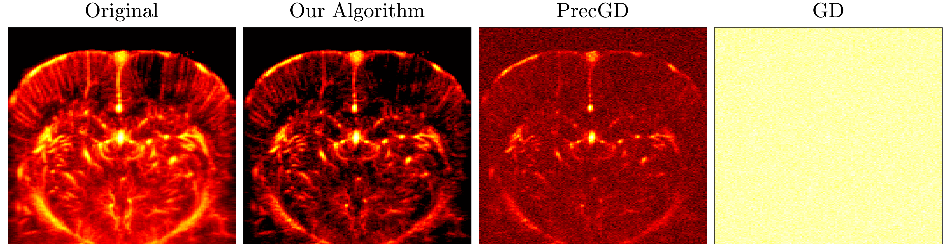
Figure 1: Ultrafast ultrasound image recovery on a scan of rat brain. We recover a 2400-frame ultrasound image ($200\times 130$ pixels per frame) under 50% downsampling rate. The ultrasound images are shown using power Doppler [1]. Left: original image. Middle-left: image recovered by our algorithm (2). Middle-right: image recovered by PrecGD. Right: image recovered by GD. All three experiments are done on a MacBook Pro 2021, with each taking approximately 3 minutes.

1.2 Related Work

Earlier work in low-rank matrix recovery focused on nuclear norm minimization [23, 8, 10, 9]. A more recent line of work uses gradient-type algorithms to solve non-convex objective (1), which has a much cheaper iteration cost compared to convex methods. When gradient descent is initialized within a neighborhood of the ground truth it is guaranteed to converge towards the ground truth $M^{\star}$ [27, 30, 2, 5, 21]. In the case where search rank $r$ is equal to the true rank $r^{\star}=\mathrm{rank}(M^{\star})$, gradient descent converges linearly to a minimax error [12]. However, the convergence rate of gradient descent is often slow in practice. In fact, gradient descent becomes increasingly slow as $M^{\star}$ becomes more ill-conditioned. In the extreme case, the search rank $r$ is greater than $r^{\star}$, so the condition number becomes infinite. This is known as the over-parameterized case, in which gradient descent slows down to a sublinear convergence rate [31].

To avoid this slow down, Tong et al. [26] proposed a method known as ScaledGD to accelerate gradient descent when the ground truth is ill-conditioned. ScaledGD converges at a linear rate independent of the condition number, but only works in the case where $r^{\star}$ is known and the measurements are noiseless. The recent work of Xu et al. [28] extends ScaledGD to also work in the over-parameterized setting by selecting a fixed regularization parameter $\lambda$. This result in an algorithm known as ScaledGD$(\lambda)$, which overcomes both ill-conditioning and over-parameterization. Moreover, ScaledGD$(\lambda)$ provably converges with a small random initialization. However, it still only works in the noiseless case. Zhang et al. [29] proposed a preconditioned version of gradient descent, known as PrecGD, which also works in the over-parmeterized regime. However, PrecGD is essentially a noiseless algorithm. In the noisy case, the authors suggest slightly adjusting $\eta_{t}$, by making calls to a hypothetical variance oracle for the measurement noise. As the authors themselves note, such an oracle is extremely expensive to implement in practice, as it amounts to some kind of resampling via a statistical technique such as cross-validation, resampling and bootstrapping. In the absence of a variance oracle, PrecGD does not converge to minimax optimality; in practice, the statistical error of PrecGD can be orders of magnitude worse than the minimax error.

2 Preliminaries

In this work we consider the symmetric, linear variant of matrix factorization known as matrix sensing which aims to recover a positive semidefinite, rank-$r^{\star}$ ground truth matrix $M^{\star}$, from a small number $m$ of possibly noisy measurements $y=\mathcal{A}(M^{\star})+\varepsilon$, where

$$\mathcal{A}(M^{\star})=[\langle A_{1},M^{\star}\rangle,\langle A_{2},M^{\star}\rangle,\dots,\langle A_{m},M^{\star}\rangle]^{T}.$$

Here $\mathcal{A}$ is a linear measurement operator, and the length-$m$ vector $\epsilon$ models the unknown measurement noise. In our theoretical analysis, we will adopt the standard assumption that $\mathcal{A}$ satisfies the restricted isometry property (RIP) [3]. We note that this is in line with existing work on the statistical optimality of gradient descent [12, 31], accelerating non-convex gradient descent [26, 29, 28] but also in line with prior work on convex methods [3, 6, 4]. Specifically, we will always assume throughout the paper that $\mathcal{A}$ satisfies RIP with parameters $(2r,\delta)$. However, we emphasize that our actual algorithm enjoy similar behavior without this assumption, as shown by our extensive simulations.

Definition 2.1 (Restricted Isometry).

The linear operator $\mathcal{A}$ satisfies RIP with parameters $(2r,\delta)$ if there exists constants $0\leq\delta<1$ and $m>0$ such that, for every rank-$2r$ matrix $M$, we have

$$(1-\delta)\|M\|_{F}^{2}\leq\frac{1}{m}\|\mathcal{A}(M)\|^{2}\leq(1+\delta)\|M\|_{F}^{2}.$$ (3)

Our goal is to recover the ground truth matrix $M^{\star}$ by using gradient descent to minimize the nonconvex loss function in (1). More importantly, we want our algorithm to converge linearly and achieve a minimax error at the same time.

Notations

We use $\|\cdot\|$ to denote the Frobenius norm and $\|\cdot\|_{2}$ to denote the spectral norm of a matrix. We use $\langle A,B\rangle=\mathrm{tr}(A^{T}B)$ to denote the standard matrix inner product. We use $\lesssim$ to denote an inequality that hides a constant factor. For a scalar function $f:\mathbb{R}^{n\times r}\to\mathbb{R}$, the gradient $\nabla f(X)$ is a matrix of size $n\times r$. For any matrix $M$, the eigenvalues and singular values are denoted by $\lambda_{i}(M)$ and $\sigma_{i}(M)$, arranged in decreasing order.

3 Failure Mechanic of Existing Algorithms

To understand why our algorithm achieves minimax optimality and immunity to ill-conditioning and over-parameterization all at the same time, it is instructive to first see how previous algorithms, especially gradient descent and PrecGD, fail in their own ways.

Exponential slowdown of gradient descent

While gradient descent converges linearly when $r=r^{\star}$, it slows down dramatically when $r^{\star}$ is not known. In the case $r=r^{\star}$, it is easy to manipulate existing results in the literature to show that the function $f(X)$ in (1) satisfies the PL-inequality, i.e., $\|\nabla f(X)\|^{2}\geq\mu f(X)$ for some positive constant $\mu>0$. Since $f(X)$ also has $\ell$-Lipschitz gradients, we get $f(X_{+})\leq f(X)-\frac{1}{2\ell}\|\nabla f(X)\|^{2}\leq\left(1-\frac{\mu}{2\ell}\right)f(X).$

We see that the convergence rate of gradient descent depends crucially on the constants $\mu$ and $\ell$. As the ground truth $M^{\star}$ becomes increasingly ill-conditioned, $\mu/L$ becomes smaller and the convergence rate becomes slow. The over-parameterized regime where $r>r^{\star}$ can be seen as an extreme case of ill-conditioning, in which case the convergence rate becomes sublinear.

PrecGD fails under noise

The recent work of [29] proposed a preconditioned variant of gradient descent called PrecGD to restore its linear convergence rate:

$$X_{t+1}=X_{t}-\alpha\nabla f(X_{t})(X_{t}^{T}X_{t}+\eta_{t}I)^{-1},\quad C_{lb}\|X_{t}X_{t}^{T}-M^{\star}\|\leq\eta_{t}\leq C_{ub}\|X_{t}X_{t}^{T}-M^{\star}\|,$$

where $C_{lb},C_{ub}$ are fixed constants. The main intuition behind this preconditioner is that it rescales the gradient so that the PL-inequality is restored. However, at the same time, the preconditioner also magnifies the Lipschitz constant of the gradient. Therefore, the regularization parameter $\eta_{t}$ plays a decisive role in maintaining both the PL-inequality and a bounded Lipschitz constant.

The key contribution of [29] is the crucial observation that the regularization parameter $\eta_{t}$ must be within a constant factor of the error $\|X_{t}X_{t}^{T}-M^{\star}\|$. In fact, they showed that $\eta_{t}$ should be small enough so that the PL-inequality is preserved, but large enough so that the gradients are still Lipschitz. Both of these properties depend on the fact that $\eta_{t}=\Theta(\|X_{t}X_{t}^{T}-M^{\star}\|)$.

In the noiseless case, simply setting $\eta_{t}=\sqrt{f(X_{t})}$ will imply $\eta_{t}=\Theta(\|X_{t}X_{t}^{T}-M^{\star}\|)$. In the noisy setting finding the right $\eta_{t}$ requires an accurate estimate of the noise variance. Unfortunately, the variance of the noise is in general very difficult to compute. In fact, the issues encountered by PrecGD here is not new and has also been observed in various other estimation methods based on $\ell_{2}$ regularization [14, 11]. In all these methods, the optimal regularization parameter becomes difficult to obtain under noise. Selecting the optimal parameter here would require an accurate estimate of the noise variance, which is often obtained based on expensive methods such as resampling, cross-validation, or bootstrapping [18, 15, 13].

Compared to PrecGD, the key feature of our method is that we no longer need to explicitly compute a regularization parameter at each iteration. Instead, it is allowed to simply decay with some fixed rate $\beta$. Surprisingly, this choice for the regularization not only eliminates the high computational cost of obtaining an accurate estimation of the noise variance, but is also capable of automatically maintaining the right amount of regularization, so that our algorithm always converges linearly, even in ill-conditioned, over-parameterized, and noisy settings.

4 Main Results

Our main result for our algorithm (2) is summarized in the theorem below. We show that under the same initial conditions as PrecGD and gradient descent [27], our algorithm converges linearly to the minimax optimal error for low-rank matrix recovery, at a rate that is independent of both ill-conditioning and over-parameterization.

Theorem 4.1.

Suppose that the initial point $X_{0}$ satisfies $\|\mathcal{A}(X_{0}X_{0}^{T}-M^{*})\|^{2}<\rho^{2}(1-\delta)\lambda_{r^{*}}(M^{\star})^{2}$. Let the step-size $\alpha$ satisfy $\alpha\leq 1/L_{P},$ where $L_{P}>0$ is a constant that only depends on $\delta$. At the $t$-th iteration, if we set the regularization parameter as $\eta_{t}=\beta^{t}\eta_{0}$, where $\eta_{0}\geq 2\sqrt{f_{c}(X_{0})}$ and $1>\beta>\sqrt{1-\frac{\mu_{p}}{4L_{P}}}$, then with high probability, we have

$$\|X_{t}X_{t}^{T}-M^{\star}\|_{F}^{2}\lesssim\max\left\{\beta^{2t}\cdot\|X_{0}X_{0}^{T}-M^{\star}\|_{F},\mathcal{E}_{opt}\right\},$$

where $\mathcal{E}_{opt}=\frac{\sigma^{2}nr\log n}{m}$. Here the inequality $\lesssim$ hides a constant that only depends on $\delta$.

A complete proof of Theorem 4.1 is presented in the appendix. In the next section, we sketch out the key ideas and lemmas behind its proof.

In Theorem 4.1, our algorithm requires an initial point that satisfies $\|\mathcal{A}(X_{0}X_{0}^{T}-M^{*})\|^{2}<\rho^{2}(1-\delta)\lambda_{r^{*}}(M^{\star})^{2}$. This requirement is standard and appears in all previous works on low-rank matrix recovery [26, 29, 12, 27] . It can be easily achieved using spectral initialization, where we simply need to compute one SVD factorization of the matrix $\mathcal{A}^{T}\mathcal{A}(y)$ [27]. Moreover, the initial value for $\eta_{t}$ can simply be set to a constant multiple of $\sqrt{f(X_{0})}.$ With high probability, this ensures that $\eta_{0}\geq 2\sqrt{f_{c}(X_{0})}$ is satisfied.

We make a few crucial observations about Theorem 4.1. First, the convergence rate is independent of both ill-conditioning and over-parameterization. In other words, this convergence rate is the same as gradient descent in the scenario where $r=r^{\star}$ and the ground truth $M^{\star}$ is perfectly conditioned. Thus, our algorithm is immune to most common dangers that causes gradient descent to stagnate in real applications. This immunity to both ill-conditioning and over-parameterization is a key feature of convex relaxation using the nuclear norm, but was lost in gradient descent. Here it is recovered again using our method.

More importantly, we note that the error that our algorithm converges to $\mathcal{E}_{opt}=O(\sigma^{2}nr\log n)$ is in indeed minimax optimal up to log factors [7]. This is the key improvement over PrecGD, whose error can be arbitrarily large depending on how well we can approximate the variance of the noise.

In Figure 2, we plot a comparison of ScaledGD$(\lambda)$, PrecGD, gradient descent (GD) and our algorithm (5.2) in two settings: (1) the noiseless, exactly-parameterized case with $r=r^{\star}$, where the ground truth $M^{\star}$ has condition number 1, and (2) the noisy, over-parameterized case with $r>r^{\star}$. In the first setting, all three algorithm perform equally well. However, in the second setting, which is much more common in the real world, our algorithm converges linearly towards a minimax error while the other two methods stagnate.

5 Key Idea and Proof Sketch of Main Results

5.1 Key Innovations

Maintaining the right amount of regularization is the most important ingredient for our method to succeed. PrecGD is successful in the noiseless setting precisely because $\eta_{t}$ is easy to compute in this setting. However, it becomes difficult if not impossible to compute in the presence of noise. This is precisely why in the noisy setting PrecGD requires a noise variance oracle that is extremely expensive to implement. Without it, PrecGD will not only lose minimax optimality, but potentially incur an arbitrarily large statistical error.

The regularization $\eta_{t}$ used in PrecGD has to be perfect because linear convergence requires two contradictory properties to intersect, namely gradient dominance (also known as the PL-inequality) and Lipschitz smoothness. When $\eta_{t}$ is too large, gradient dominance is lost. When $\eta_{t}$ is too small, Lipschitz smoothness is lost. The analysis in suggests that the choice of $\eta_{t}$ is extremely fragile and delicate. Surprisingly, we find that this is not the case. In fact, we will show that the choice of $\eta_{t}$ is not delicate, but rather robust. Our method avoids the need to choose the optimal regularization parameter altogether by simply letting $\eta$ decay with some rate $\beta<1$. It turns out that this extremely simple choice of the regularization parameter will automatically maintain the right amount of regularization needed for linear convergence due to a phenomenon we call ’coupling’.

This phenomenon can be intuitively understood as a race in which the two runners $\eta_{t}$ and $\mathcal{E}_{t}{=}\|X_{t}X_{t}^{T}-M^{\star}\|_{F}$, are connected using a rubber band. When $\eta_{t}$ and $\mathcal{E}_{t}$ begin to grow apart, the rubber band will exert a counteracting force and pull them back together. As a result, the amount of regularization is always right. This happens because that $\eta_{t}$ itself controls how fast $\mathcal{E}_{t}$ decays. If the regularization parameter $\eta_{t}$ is large compared to $\mathcal{E}_{t}$, then our algorithm behaves more like gradient descent, because the second term in $X_{t}^{T}X_{t}+\eta_{t}\cdot I$ will dominate the first. As a result, our algorithm becomes similar to gradient descent and begins to briefly stagnate: the error $\mathcal{E}_{t}$ decays slowly, allowing $\eta_{t}$ to catch up and become close to $\mathcal{E}_{t}$ again. Similarly, if $\eta_{t}$ is small, then the first term in the preconditioner dominates, causing our algorithm to converge faster. Thus, the error $\mathcal{E}_{t}$ decays quickly, and will eventually catch up to $\eta_{t}$.

This coupling of the regularizaton parameter and the error is precisely why we can avoid the expensive procedure used in PrecGD to estimate the noise variance and approximate $\mathcal{E}_{t}$. We implicitly maintain the right amount of regularization, so that our algorithm always converges linearly, even in ill-conditioned, over-parameterized, and noisy settings.

5.2 Proof Sketch

In this section we sketch the main steps of the proof of our main result, Theorem 4.1, and defer the full proof to the appendix. Our proof consists of two components: the first is the observation that the PL-inequality, which is lost in the case $r>r^{\star}$, can be restored under a change of norm, as long as the preconditioner $P=(X_{t}^{T}X_{t}+\eta_{t}\cdot I)^{-1}$ has the “correct” amount of regularization $\eta_{t}$. The second component is the observation that $\eta_{t}$ and $\mathcal{E}_{t}=\|X_{t}X_{t}^{T}-M^{\star}\|$ are coupled together, meaning that they can never be too far apart.

For brevity, we only outline the important intermediate results in our proof below. To begin, note that the objective function in (1) can be written as

$$f(X)=\frac{1}{m}\|\mathcal{A}(XX^{T})-y\|^{2}=f_{c}(X)+\frac{1}{m}\|\varepsilon\|^{2}-\frac{2}{m}\langle\mathcal{A}(XX^{T}-M^{\star}),\varepsilon\rangle,$$

where $f_{c}(X)=\frac{1}{m}\|\mathcal{A}(XX^{T}-M^{\star})\|^{2}$ is defined to be the objective function with clean measurements that are not corrupted by noise.

The first component in our proof consists of showing that the iterates of 2 can be viewed as gradient descent under a change of norm. In particular, let $P=X^{T}X+\eta_{t}\cdot I$ be a real symmetric, positive definite $r\times r$ matrix. We define a corresponding $P$-norm and its dual $P$-norm on $\mathbb{R}^{n\times r}$ as follows

$$\|X\|_{P}\overset{\text{def}}{=}\|XP^{1/2}\|,\quad\|X\|_{P*} \overset{\text{def}}{=}\|XP^{-1/2}\|.$$ (4)

Consider the descent direction $D=\nabla f_{c}(X)P^{-1}$. Suppose that we can show that the following inequality holds with some constant $L_{p}$:

$$f_{c}(X-\alpha D)\leq f_{c}(X)-\alpha\langle\nabla f_{c}(X),D\rangle+\frac{\alpha^{2}L_{P}}{2}\|D\|_{P}$$ (5)

Then plugging $D=\nabla f_{c}(X)P^{-1}$ into the inequality above and setting $\alpha=1/L_{p}$ yields $f(X-\alpha\nabla f_{c}(X)P^{-1})\leq f_{c}(X)-\frac{1}{2L_{p}}\|\nabla f_{c}(X)\|_{P*}^{2}.$ Now suppose that the PL-inequality holds under the dual $P$-norm, $\|\nabla f_{c}(X)\|_{P*}^{2}\geq\mu_{P}(f_{c}(X))\quad\text{ where }\mu_{P}>0$ then we have the desired linear convergence since $f_{c}(X-\alpha D)\leq\left(1-\frac{\mu_{p}}{2L_{p}}\right)f_{c}(X).$ Therefore, to complete our proof, we need to demonstrate the following conditions. For $P=X_{t}^{T}X_{t}+\eta_{t}I$, we have

1. The inequality (5) holds with some constant $L_{p}$, or equivalently, the gradient $\nabla f_{c}(X)$ is Lipschitz under the $P$-norm.

2. The PL-inequality holds under the $P$-norm: $\|\nabla f_{c}(X)\|_{P*}^{2}\geq\mu_{P}(f_{c}(X))$.

Finally, since the measurements are noisy, we only have access to the noisy gradient $\nabla f(X)$ at each iteration, instead of the “true” gradient $\nabla f_{c}(X)$, we need to show that the difference between $\nabla f_{c}(X)$ and $\nabla f(X)$ is small.

First, we consider an ideal case, where the three issues above are easier to resolve: suppose that there exists some constant $C>1$ such that $\eta_{t}\leq\sqrt{f_{c}(X_{t})}\leq C\eta_{t}$. This is exactly the regime for $\eta_{t}$ where our algorithm is well-behaved: both Lipschitz gradients and the PL-inequality is satisfied in the $P$-norm. In fact, we will see that the Lipschitz constant for the gradients (in the $P$-norm) can be bounded as

$$L_{P}\lesssim\left(\|XX^{T}-M^{\star}\|_{F}/\lambda_{\min}(X^{T}X)+\eta\right)^{2}.$$

Therefore, if $\sqrt{f_{c}(X_{t})}\leq C\eta_{t}$, then $L_{p}$ is bounded, which implies that inequality (5) holds. On the other hand, if $\eta_{t}\leq\sqrt{f_{c}(X_{t})}$, then $\|\nabla f_{c}(X)\|_{P*}^{2}\geq\mu_{P}(f_{c}(X))$. The proof of these two facts, especially the second one, is quite involved, but it is similar to the proof of Corollary 5 in [29], so they are deferred to the appendix.

As a result, in the ideal case where $\eta_{t}\leq\sqrt{f_{c}(X_{t})}\leq C\eta_{t}$, if we go in the direction $D=\nabla f_{c}(X)P^{-1}$, then linear convergence is already achieved. However, due to noise, the descent direction is $\nabla f(X)$, instead of $\nabla f_{c}(X)$, since we cannot access the true gradient. Fortunately, if the norm of the gradient is large compared to a statistical error, then the difference between $\nabla f_{c}(X)$ and $\nabla f(X)$ is negligible, and our algorithm will still make enough progress at each iteration to ensure linear convergence. This is summarized in the lemma below.

Lemma 5.1.

Suppose that at the $t$-th iteration, we have $\eta_{t}\leq\sqrt{f_{c}(X_{t})}\leq C\eta_{t}$ for some constant $C>1$. Furthermore, suppose that $\|\nabla f_{c}(X_{t})\|_{P}^{*}\gtrsim\sqrt{\frac{\sigma^{2}rn\log n}{m}}.$ Then for step-size $\alpha\leq 1/L_{p}$, with high probability we have

$$f_{c}(X_{t+1}) \leq\left(1-\frac{\mu_{P}}{2L_{p}}\right)f_{c}(X_{t}).$$

Here $L_{p}=O(C^{2})$ is a constant that only depends on $\delta$ and $C$.

The proof of Lemma 5.1 can be found in the appendix. Essentially, it states that if $\eta_{t}\approx\sqrt{f_{c}(X_{t})}$, then our algorithm will converge linearly up to some statistical error. Therefore, if $\eta_{t}\approx\sqrt{f_{c}(X_{t})}$ always holds, then the proof is already complete. Unfortunately, this is not the case, because both $\eta_{t}$ and $\sqrt{f_{c}(X_{t})}$ are changing. At time $t+1$, the ideal condition that $\eta_{t+1}\leq\sqrt{f_{c}(X_{t+1})}\leq C\eta_{t+1}$ might no longer be satisfied, so Lemma 5.1 is no longer applicable. Instead, we have to consider scenarios where $\eta_{t}$ deviates from this ideal range. To complete the proof of Theorem 4.1, we need to show that $\eta_{t}$ never deviates too far from the ideal range in which Lemma 5.1 is applicable. Intuitively, if $\sqrt{f_{c}(X_{t+1})}$ becomes too small compared to $\eta_{t}$, our algorithm will start to behave more like gradient descent and slow down. Hence with a fixed decay rate, $\eta_{t}$ will quickly be on the same order as $\sqrt{f_{c}(X_{t+1})}$ again, so that Lemma 5.1 can be applied again. As a result, linear convergence is always maintained.

6 Numerical Simulations

In this section we provide numerical experiments to validate our theoretical results: our algorithm (2) converges linearly to a minimax optimal error of $O(\sigma^{2}nr)$. In comparison, GD struggles to decrease the error due to a sublinear convergence rate in the over-parameterized regime, and both PrecGD [29] and ScaledGD$(\lambda)$ [28] converge to an error that is not minimax optimal.

We also perform experiments to gauge the performance of our algorithm for applications outside of the assumptions of our theoretical results. To begin, we consider two common problems considered in the existing literature that do not satisfy conditions under which Theorem 4.1 applies: phase retrieval and 1-bit matrix sensing. For these problems, we see almost identical results to low-rank matrix recovery: our algorithm succeeds in converging to a minimax optimal error, while GD, PrecGD and ScaledGD$(\lambda)$ struggle. Finally, we consider a real-world medical imaging application, specifically in ultrafast ultrasound, where we see that our algorithm significantly outperforms competing methods in achieving the highest accuracy within a short amount of computing time. Thus, we believe that our algorithm is widely applicable to many practical problems whose measurements do not satisfy the restricted isometry property. However, we leave a rigorous justification of these observations for future work.

Experimental setups

We perform our experiments on an Apple MacBook Pro, running a silicon M1 pro chip with 10-core CPU, 16-core GPU, and 32GB of RAM. We implement our algorithm in MATLAB R2021a.

Gaussian matrix sensing

In this experiment, we consider a matrix recovery problem on a $10\times 10$ ground truth matrix $M^{\star}$ with truth rank $r^{\star}=2$. The condition number of $M^{\star}$ is set to $\kappa=1$. We take $m=80$ measurements on $M^{\star}$ using $m$ linearly independent measurement matrices $A_{1},\ldots,A_{m}$ drawn from the standard Gaussian distribution. In Figure 2, we plot the convergence of our algorithm, PrecGD, ScaledGD$(\lambda)$ and GD under two settings: the exactly-parameterized, noiseless case; and the over-parameterized, noisy case. In both settings, we start the four methods at the same random initial point $X_{0}$ with a learning rate $\alpha=10^{-1}$. The first setting corresponds to the case where $r^{\star}$ is known, and our measurements are perfect. In this highly unrealistic scenario, we see that the all four methods behave identically, converging linearly to machine error. In the second setting, we set the search rank to be $r=4$, and we corrupt the measurements with noise $\varepsilon\sim\mathcal{N}(0,\sigma^{2})$ where $\sigma=10^{-6}$. For our algorithm, we set $\eta_{0}=\sqrt{f(X_{0})}$ and the decay rate for $\eta_{t}$ as $\beta=0.1$. Here PrecGD is implemented with a proxy variance $\hat{\sigma}$ that is within a small constant factor of $\sigma$, so that $\eta_{t}=\sqrt{|f(X_{t})-\hat{\sigma}^{2}|}$, and ScaledGD$(\lambda)$ is implemented with $\lambda=10^{-2}$. We note that we pick $\lambda$ according to Assumption 2 in [28]. We see that our algorithm converges to a minimax error of around $10^{-6}$, while PrecGD, ScaledGD$(\lambda)$ and GD struggles to attain the same error. Here the slow down of GD is due to over-parameterization, while the showdown of PrecGD and ScaledGD$(\lambda)$ are due to an inaccurate estimate of scaling parameters.

Figure 2: Convergence of our algorithm, PrecGD, ScaledGD$(\lambda)$ and GD for Gaussian matrix sensing. Left: Noiseless measurements with $r=r^{\star}$. Right: Noisy measurements with $r>r^{\star}$.

1-bit Matrix Sensing

We take the same ground truth matrix $M^{\star}$ in Gaussian matrix sensing to perform experiment on 1-bit matrix sensing [19]. For 1-bit matrix sensing, the measurements $y_{ij}$ of each entry of $M^{\star}$ are quantized, so that they are $1$ with some probability $\sigma(M_{ij}^{\star})$ and $0$ with probability $1-\sigma(M_{ij}^{\star})$ where $\sigma(\cdot)$ is the sigmoid function. We leave the details of this experiment to the appendix. Again, we see that the results are almost identical to that of low-rank matrix recovery: our algorithm is able to converge linearly to a minimax error rate as soon as $r>r^{\star}$, but PrecGD, ScaledGD$(\lambda)$ and GD showdown dramatically.

Figure 3: Convergence of our algorithm, PrecGD, ScaledGD$(\lambda)$ and GD for 1-bit matrix sensing. Left: Noiseless measurements with $r=r^{\star}$. Right: Noisy measurements with $r>r^{\star}$.

Phase Retrieval

We perform experiment on phase retrieval [9] using a length 10 complex ground truth vector $z$. The goal of phase retrieval is to recover $z$ from phaseless measurements of the form $y_{i}=|\langle a_{i},z\rangle|^{2}$, where the $a_{i}$ are measurement vectors in $\mathcal{C}^{10}$. This problem can be viewed as recovering a size $10\times 10$ complex ground truth matrix $M^{\star}$ from measurements $y_{i}=\langle a_{i}a_{i}^{T},M^{\star}\rangle$, subjecting to a constraint that $M$ is rank-1. In this experiment, we randomly generate $m=80$ measurement vectors $a_{1},\ldots,a_{m}$ where the real and imaginary part of $a_{i}$ are drawn from standard Gaussian. We leave the details of this experiment to the appendix. Figure 4 shows the convergence of our alogirthm, PrecGD, ScaledGD$(\lambda)$ and GD. Again, our algorithm again converge linearly to the minimax error.

Figure 4: Convergence of our algorithm, PrecGD, ScaledGD$(\lambda)$ and GD for phase retrieval. Left: Noiseless measurements with $r=r^{\star}$. Right: Noisy measurements with $r>r^{\star}$.

Ultrafast ultrasound image recovery

We are interested in recovering a 60 megapixel (2400-frames, $200\times 130$ pixels per frame) ultrafast ultrasound image under 50% downsampling rate. This problem often arises in real-time ultrasound image acquisition because without downsampling, managing a vast amount of data associated with high frame rate posts a critical challenge on communication bandwidth and data storage devices. In this case, the ultrasound image recovery problem can be viewed as estimating a size $26000\times 2400$ ground truth matrix $M^{\star}$ from 31.2 million noisy measurements on its entries. Here the $i$-th column of $M^{\star}$ corresponds to the vectorization of the $i$-th frame in the ultrasound scan. We leave the details of this experiment to the appendix. In Figure 1, we show the ultrasound image recovered from our algorithm, PrecGD and GD in power Doppler [1]. As shown in Figure 1, our algorithm is the only algorithm that is able to almost perfectly recover the original image, while also applying a denoising effect, making the image even sharper. We also emphasize that the per-iteration cost of our algorithm is almost identical to gradient descent. All three experiments take approximately 3 minutes.

7 Acknowledgements

The authors are grateful to Salar Fattahi for helpful discussions and valuable insights regarding achieving minimax error for this problem. We are also are grateful to Pengfei Song and YiRang Shin for their help and advice on the ultrafast ultrasound application, and for sharing the rat brain datasets used in our medical imaging experiments. Financial support for this work was provided in part by NSF CAREER Award ECCS-2047462.

Appendix A Proof of Main Results

A.1 Preliminaries

First we introduce some notations and lemmas from previous works that we will use in the proof of Lemma 5.1 and Theorem 4.1.

For matrix sensing, we note our ground truth by $M^{\star}=ZZ^{T}\in\mathbb{R}^{n\times n}$. Our goal is to recovery $M^{\star}$ from a small number of measurements of the form $y=\mathcal{A}(ZZ^{T})+\epsilon\in\mathbb{R}^{m}$. Here $\epsilon$ is a vector with sub-Gaussian entries with zero mean and variance $\sigma^{2}=\frac{1}{m}\sum_{i=1}^{m}\mathbb{E}[\epsilon_{i}^{2}]$. To do so, we minimize the non-convex objective function

$$f(X)=\frac{1}{m}\|\mathcal{A}(XX^{T})-y\|^{2}=f_{c}(X)+\frac{1}{m}\|\epsilon\|^{2}-\frac{2}{m}\langle\mathcal{A}(XX^{T}-M^{\star}),\epsilon\rangle,$$

where $f_{c}(X)\overset{def}{=}\frac{1}{m}\|\mathcal{A}(XX^{T}-M^{\star})\|^{2}$ is the objective function with clean measurements that are not corrupted with noise.

We make a few simplifications on notations. As before, we will use $\alpha$ to denote the step-size and $D$ to denote the local search direction. In our proof below, it will often be easier to use the vectorized form of our gradient updates:

$$\operatorname*{\mathrm{vec}}{X_{t+1}} =\operatorname*{\mathrm{vec}}{X_{t}}-\alpha\operatorname*{\mathrm{vec}}{\nabla f(X_{t})(X_{t}^{T}X_{t}+\eta_{t}I)^{-1}}$$

$$=\operatorname*{\mathrm{vec}}X_{t}-((X_{t}^{T}X_{t}+\eta_{t}I)\otimes I)^{-1}\operatorname*{\mathrm{vec}}(\nabla f(X_{t})),$$

where in the second line we used the standard identity $\operatorname*{\mathrm{vec}}(AXB)=(B^{T}\otimes A)\operatorname*{\mathrm{vec}}(X)$ for the Kronecker product $\otimes$. For simplicity, we will use lower case letters $x$ and $d$ to refer to $\operatorname*{\mathrm{vec}}{(X)}$ and $\operatorname*{\mathrm{vec}}{(D)}$ respectively. We will also write $\nabla f(x_{t})$ as the vectorized form of $\nabla f(X_{t})$. Then the update above can be written as $x_{t+1}=x_{t}-\alpha\mathbf{P}^{-1}\nabla f(x_{t})$, with $\mathbf{P}=(X_{t}^{T}X_{t}+\eta_{t}I)\otimes I$.

A.2 Auxiliary Results

In this section we collect two results from [29] that will be used in the proof of our main result. The first theorem shows that when the regularization $\eta$ is small, the PL-inequality holds within a small neighborhood around the ground truth.

Theorem A.1 (Noiseless gradient dominance).

Let $\min_{X}f(X)=0$ for $M^{\star}\neq 0$. Suppose that $X$ satisfies $f(X)\leq\rho^{2}\cdot(1-\delta)\lambda_{r^{\star}}^{2}(M^{\star})$ with radius $\rho>0$ that satisfies $\rho^{2}/(1-\rho^{2})\leq(1-\delta^{2})/2$. Then, we have

$$\eta\leq C_{ub}\|XX^{T}-M^{\star}\|_{F}\quad\implies\quad\|\nabla f(X)\|_{P*}^{2}\geq 2\mu_{P}f(X)$$

where

$$\mu_{P}=\left(\sqrt{\frac{1+\delta^{2}}{2}}-\delta\right)^{2}\cdot\min\left\{\left(\frac{C_{1}}{\sqrt{2}-1}\right)^{-1},\left(1+3C_{1}\sqrt{\frac{(r-r^{\star})}{1-\delta^{2}}}\right)^{-1}\right\}.$$ (6)

Here $C_{1}$ is a constant that only depend on $\delta$.

We recall that in the theorem above $\|\cdot\|_{P^{*}}$ denotes the dual norm of $\|\cdot\|_{P}$ defined in (4), with $P=X^{T}X+\eta I$. Essentially, this theorem says that when $\eta$ is small compared to the true error $\|XX^{T}-M^{\star}\|$, the PL-inequality is restored under the local norm defined by $P$. The difficulty of applying this theorem directly in our case arises from two issues: first, if $\eta$ is too small, then the gradients of $f(X)$ are no longer Lipschitz under the $P$-norm. As a result, the iterates can diverge. Moreover, it is very difficult to gauge the ‘right’ size of $\eta$ in the noisy setting, since we have no access to the true error. The proof of Theorem A.1 can be found in [29] so we do not repeat it here.

We also state an lemma from [29] that directly characterizes the progress of gradient descent at each iteration in a fashion similar to the descent lemma (see e.g. [22]). For general smooth functions with Lipschitz gradients, the decrement in the function value at each iteration can be characterized by a quadratic upper bound (the so-called descent lemma). However, for matrix sensing, we can in fact obtain a tighter upper bound because $f_{c}(X-\alpha D)$ itself is just a quartic polynomial. This allows us to characterize the progress made at each iteration directly, using the following result.

Lemma A.2.

For any descent direction $D\in\mathbb{R}^{n\times r}$ and step-size $\alpha>0$ we have

$$f_{c}(X-\alpha D) \leq f_{c}(X)-\alpha\langle\nabla f_{c}(X),D\rangle+\frac{\alpha^{2}}{2}\langle D,\nabla^{2}f_{c}(X)[D]\rangle$$ (7)

$$+\frac{(1+\delta)\alpha^{3}}{m}\|D\|_{F}^{2}\left(2\|DX^{T}+XD^{T}\|_{F}+\alpha\|D\|_{F}^{2}\right).$$ (8)

The proof of this lemma is quite straightforward so we do not repeat it here. The Lemma follows simply from expanding the function $f_{c}(X-\alpha D)$ and bounding the third and fourth order terms using the restricted isometry property of $\mathcal{A}$.

A.3 Proof of Lemma 5.1

For the PrecGD algorithm of [29] to succeed, it is crucial that the regularization parameter satisfies $\eta_{t}\leq\sqrt{f_{c}(X_{t})}\leq C\eta_{t}$. If so, then within a local neighborhood of the ground truth, Theorem A.1 and Theorem A.2 can be used to establish linear convergence in the noiseless setting. However, as we have argued in the main paper, this requirement for $\eta_{t}$ is difficult if not impossible to maintain explicitly in the noisy setting. This makes it extremely difficult for PrecGD to achieve a minimax optimal error.

Our main result, Theorem 4.1, states that letting $\eta_{t}$ decay with some constant rate $\beta$ suffices to guarantee the linear convergence of our algorithm, even in the noisy setting. One of our key observations is that the condition $\eta_{t}\leq\sqrt{f_{c}(X_{t})}\leq C\eta_{t}$ does not have to be satisfied at all times. In fact, we can allow $\eta_{t}$ to dip below $\sqrt{f_{c}(X_{t})}$ in our algorithm, because of the “coupling” effect that we discussed previously: $\eta_{t}$ can never deviate too far from $\sqrt{f_{c}(X_{t})}$.

Therefore, in our proof of Theorem 4.1, we will consider two cases:

1. $\eta_{t}\leq\sqrt{f_{c}(X_{t})}\leq C\eta_{t}$

2. $\sqrt{f_{c}(X_{t})}\leq\eta_{t}$.

The first case is the “good” situation, because the conditions under which PrecGD converges linearly is satisfied by assumption. In this case, we show that as long as the gradient is large compared to the noise, i.e., $\|\nabla f_{c}(X_{t})\|_{P}^{*}\gtrsim\sqrt{\frac{\sigma^{2}rn\log n}{m}},$ our algorithm will converge linearly for precisely the same reasons that PrecGD converges linearly. This behavior is stated rigorously in Lemma 5.1, which we restate below.

Lemma A.3 (Lemma 5.1 restated).

Suppose that at the $t$-th iteration, we have $\eta_{t}\leq\sqrt{f_{c}(X_{t})}\leq C\eta_{t}$ for some $C>1$. Furthermore, suppose that $\|\nabla f_{c}(X_{t})\|_{P}^{*}\gtrsim\sqrt{\frac{\sigma^{2}rn\log n}{m}}.$ Then for $\alpha\leq 1/L_{p}$, with high probability we have

$$f_{c}(X_{t+1}) \leq\left(1-\frac{\mu_{P}}{2L_{p}}\right)f_{c}(X_{t}).$$

Here $L_{p}=O(C^{2})$ is a constant that only depends on $\delta$ and $C$.

The proof of Lemma 5.1 is long but it is mainly computational. The overall idea is similar to the proof of Theorem 20 in [29]: our goal is to show that when the local norm of the gradient is large compared to the noise level, the decrement we make at each iteration ‘overcomes’ the error caused by the noisy measurements. Our main tool here is Lemma A.2, which allows us to directly compute the decrement and bound the error terms.

It turns out that in this proof, it will be slightly easier to deal with the vectorized version of this problem: we use $f(x)$ to denote original objective function $f(X)$ as a function of the vector $x=\operatorname*{\mathrm{vec}}(X)$. Consequently, we write $f(x)\in\mathbb{R}^{nr}$ and $\nabla f(x)\in R^{nr}$ as the vectorized versions of $f(X)$ and its gradient. We use the same vectorized notation for the “true” function value $f_{c}(X)$. Thus, in vectorized form, the iterates of our algorithm can be written as

$$x_{k+1}=x_{k}-\alpha\mathbf{P}^{-1}\nabla f(x),\quad\text{where }\mathbf{P}=(X^{T}X+\eta I_{r})\otimes I_{n}.$$

We note that all the norms we consider remain unchanged after vectorization, meaning that $\|\nabla f(x)\|_{P}=\|\nabla f(X)\|_{P}$ and $\|\nabla f(x)\|_{P^{*}}=\|\nabla f(X)\|_{P^{*}}.$ Now we are ready to prove this lemma.

Proof.

The main idea of the proof is to use the inequality $\eta_{t}\leq\sqrt{f_{c}(X_{t})}\leq C\eta_{t}$ to bound the progress of our algorithm at each iteration. In particular, when $\eta_{t}$ is small, i.e., $\eta_{t}\leq\sqrt{f_{c}(X_{t})}$, then Theorem A.1 guarantees the gradient dominance. On the other hand, the lower bound $\sqrt{f_{c}(X_{t})}\leq C\eta_{t}$ allows us to apply Lemma A.2 to guarantee that the step-size $\alpha$ can be large enough so that we get linear convergence.

First, note that vectorized version of the gradient update $X_{+}=X-\alpha D$ (where $D=\nabla f(X)P^{-1}$) can be written as $x_{+}=x-\alpha d$, where

$$d =\operatorname*{\mathrm{vec}}{(\nabla f(X)P^{-1})} =\mathbf{P}^{-1}\nabla f_{c}(x)-\frac{2}{m}\mathbf{P}^{-1}\left(I_{r}\otimes\sum_{i=1}^{m}\epsilon_{i}A_{i}\right)x.$$ (9)

Here we have dissected the gradient descent direction into two parts: $\mathbf{P}^{-1}\nabla f_{c}(x)$, which corresponds to “correct” gradient and a remaining error term $\mathbf{P}^{-1}\mathcal{E}(x)$, where

$$\mathcal{E}(x)\overset{def}{=}\frac{2}{m}\left(I_{r}\otimes\sum_{i=1}^{m}\epsilon_{i}A_{i}\right)x.$$

In other words we have $d=\mathbf{P}^{-1}(\nabla f_{c}(x)-\mathcal{E}(x))$. If $\mathcal{E}(x)=0$, then our proof reduces to the noiseless case. Here we want to show that the error is small compared the decrement we make in the function value. As we will see, this happens precisely in the regime where the gradient is large, i.e., $\|\nabla f_{c}(X)\|_{P}^{*}\gtrsim\sqrt{\frac{\sigma^{2}rn\log n}{m}}.$

In vectorized notation, Lemma A.2 can be written as

$$f_{c}(x-\alpha d)\leq f_{c}(x)-\alpha\nabla f_{c}(x)^{T}d+\frac{\alpha^{2}}{2}d^{T}\nabla^{2}f_{c}(x)d+\frac{(1+\delta)\alpha^{3}}{m}\|d\|^{2}\left(2\|\mathbf{J}d\|+\alpha\|d\|^{2}\right),$$ (10)

where we define $\mathbf{J}:\mathbb{R}^{nr}\to\mathbb{R}^{n^{2}}$ as the linear operator satisfying $\mathbf{J}d=\operatorname*{\mathrm{vec}}(XD^{T}+DX^{T})$ (recall that $d=\operatorname*{\mathrm{vec}}(D)$). Now setting $d=\mathbf{P}^{-1}(\nabla f_{c}(x)-\mathcal{E}(x))$ in the formula above yields

$$f_{c}(x-\alpha d)\leq f_{c}(x)-\alpha\|\nabla f_{c}(x)\|_{P*}^{2}+T_{1}+T_{2}+T_{3}$$

where

$$T_{1}= \alpha\nabla f_{c}(x)^{T}\mathbf{P}^{-1}\mathcal{E}(x)$$

$$T_{2}= \frac{\alpha^{2}}{2}\Big{(}\nabla f_{c}(x)^{T}\mathbf{P}^{-1}\nabla^{2}f_{c}(x)\mathbf{P}^{-1}\nabla f_{c}(x)+\mathcal{E}(x)^{T}\mathbf{P}^{-1}\nabla^{2}f_{c}(x)\mathbf{P}^{-1}\mathcal{E}(x)$$

$$-2\nabla f_{c}(x)^{T}\mathbf{P}^{-1}\nabla^{2}f_{c}(x)\mathbf{P}^{-1}\mathcal{E}(x)\Big{)}$$

$$T_{3}= (1+\delta)\alpha^{3}\left(\|\mathbf{P}^{-1}\nabla f_{c}(x)-\mathbf{P}^{-1}\mathcal{E}(x)\|^{2}\right)\left(2\|\mathbf{J}\mathbf{P}^{-1}\nabla f_{c}(x)\|+2\|\mathbf{J}\mathbf{P}^{-1}\mathcal{E}(x)\|\right.$$

$$+\left.\alpha\|\mathbf{P}^{-1}\nabla f_{c}(x)-\mathbf{P}^{-1}\mathcal{E}(x)\|^{2}\right).$$

Our goal is to show that all three terms $T_{1},T_{2},T_{3}$ are small compared to the decrement that we make at each iteration. The key observation here is that all of these terms depend on $\mathcal{E}(x)$ and $\mathbf{P}$. With the right choice of $\eta$, i.e., with $\sqrt{f_{c}(X_{t})}\leq C\eta_{t}$, the preconditioner $\mathbf{P}$ is well-conditioned, so that all the errors in $T_{1},T_{2},T_{3}$ will remain small as long as $\mathcal{E}(x)$ is small. Specifically, we can bound the error term as

$$\|\mathcal{E}(x)\|_{P^{*}}^{2} =\mathcal{E}(x)^{T}\mathbf{P}^{-1}\mathcal{E}(x)=\left\|\left(\frac{2}{m}\sum_{i=1}^{m}\epsilon_{i}A_{i}\right)X(X^{T}X+\eta I)^{-1/2}\right\|_{F}^{2}$$

$$\leq\left\|\left(\frac{2}{m}\sum_{i=1}^{m}\epsilon_{i}A_{i}\right)\right\|_{2}^{2}\left\|X(X^{T}X+\eta I)^{-1/2}\right\|_{F}^{2}$$

$$\overset{(i)}{}\leq C_{e}\frac{\sigma^{2}n\log n}{m}\left(\sum_{i=1}^{r}\frac{\sigma_{i}^{2}(X)}{\sigma_{i}(X)^{2}+\eta}\right)$$

$$\leq C_{e}\frac{\sigma^{2}rn\log n}{m},$$

where (i) follows from a standard concentration bound (see [7]).

Now, denoting $\Delta=\|\nabla f_{c}(x)\|_{P*}$ and using the bound for the error above, we get after some computations that

$$T_{1}\leq\alpha\Delta\sqrt{\frac{C_{e}\sigma^{2}rn\log n}{m},}$$

$$T_{2}\leq 2\alpha^{2}L_{\delta}\Delta^{2}+2\alpha^{2}L_{\delta}\frac{\sigma^{2}rn\log n}{m}$$

$$T_{3}\leq\frac{4(1+\delta)\alpha^{3}}{\eta}\left(\Delta^{2}+\frac{C_{e}\sigma^{2}rn\log n}{m}\right)\left(\frac{\alpha\Delta^{2}}{\eta}+\frac{\alpha C_{e}\sigma^{2}rn\log n}{\eta m}+2\sqrt{2}\Delta+2\sqrt{2}\sqrt{\frac{C_{e}\sigma^{2}rn\log n}{m}}\right).$$

Here $C_{e}$ is a absolute constant and $L_{\delta}$ is a constant that depends only on the RIP constant $\delta$. Now plugging these error bounds back into (11) yields

$$f_{c}(x-\alpha d) \leq f_{c}(x)-\alpha\Delta^{2}+\alpha\Delta\sqrt{\frac{C\sigma^{2}rn\log n}{m}}+2\alpha^{2}L_{\delta}\Delta^{2}+2C\alpha^{2}L_{\delta}\frac{\sigma^{2}rn\log n}{m}$$

$$+\frac{4(1+\delta)\alpha^{3}}{\eta}\left(\Delta^{2}+\frac{C\sigma^{2}rn\log n}{m}\right)\left(\frac{\alpha\Delta^{2}}{\eta}+\frac{\alpha C\sigma^{2}rn\log n}{\eta m}+2\sqrt{2}\Delta+2\sqrt{2}\sqrt{\frac{C\sigma^{2}rn\log n}{m}}\right).$$ (11)

In the case $\Delta\geq 2\sqrt{\frac{C_{e}\sigma^{2}rn\log n}{m}}$ all the terms above can be bounded so that the decrement in the function value dominates all the error. In particular, plugging this lower bound into the inequality above yields

$$f_{c}(x-\alpha d)\leq f_{c}(x)-\frac{\alpha}{2}\Delta^{2}\left(1-\frac{5}{2}L_{\delta}\alpha-60\sqrt{2}\alpha^{2}(1+\delta)-25\alpha^{3}(1+\delta)^{2}\right).$$

Now, assuming that the step-size satisfies

$$\alpha\leq\min\left\{\frac{L_{\delta}}{60\sqrt{2}(1+\delta)+25(1+\delta)^{2}},\frac{1}{7L_{\delta}}\right\}\overset{def}{=}\frac{1}{L_{P}}$$ (12)

we obtain $f_{c}(x-\alpha d)\leq f_{c}(x)-\frac{t\Delta^{2}}{4}\leq\left(1-\frac{\alpha\mu_{P}}{4}\right)f_{c}(x),$ where in the last step we used the fact that $\eta_{t}\leq\sqrt{f_{c}(X_{t})}$, so the conditions of Theorem A.1 are satisfied, so gradient dominance holds. This completes the proof.

∎

Appendix B Proof of Theorem 4.1

In this section we provide a complete proof of Theorem 4.1, filling out some of the missing details left out in the main paper.

Proof.

Let $T>0$ be the smallest index such that $\eta_{T}<2\sqrt{\frac{C_{0}\sigma^{2}rn\log n}{\mu_{p}m}}$. Suppose that $t<T$. Similar to the noiseless case, we will show that there exists some constant $C>1$, which depends only on $\delta$, such that the following holds: if at the $t$-th iterate we have $\sqrt{f_{c}(X_{t})}\leq C\eta_{t}$, then $\sqrt{f_{c}(X_{t+1})}\leq C\eta_{t+1}$. As before, this implies that $f_{c}(X_{t})\leq C^{2}\beta^{2t}\eta_{0}$ for all $t\leq T$.

At the $t$-iterate, suppose that $\sqrt{f_{c}(X_{t})}\leq C\eta_{t}$. We consider two cases:

1. $\eta_{t}\leq\sqrt{f_{c}(X_{t})}\leq C\eta_{t}$

2. $\sqrt{f_{c}(X_{t})}\leq\eta_{t}$.

We will show that in either case, the next iterate satisfies $\sqrt{f_{c}(X_{t+1})}\leq C\eta_{t+1}.$ The core idea behind this proof is that the values of $\eta_{t}$ and $\sqrt{f_{c}(X_{t+1})}$ are “coupled”, meaning that they can not deviate too far from each other. In the first case, where $\eta_{t}\leq\sqrt{f_{c}(X_{t})}\leq C\eta_{t}$, the behavior of our algorithm plus is exactly the same as PrecGD, since $\eta_{t}$ is bounded both above and below by a constant factor of $\sqrt{f_{c}(X_{t+1})}$. Thus, according to Lemma 5.1, we converge linearly (at least for the current iteration). In fact, we have chosen the decay rate $\beta$ so that $f_{c}(X)$ will decay faster than $\beta$ when $\eta_{t}\leq\sqrt{f_{c}(X_{t})}\leq C\eta_{t}$. Specifically, we have

$$\sqrt{f_{c}(X_{t+1})}\leq\sqrt{\left(1-\frac{\mu_{P}}{4L_{p}}\right)}\sqrt{f_{c}(X_{t})}\leq\beta\cdot C\eta_{t}=C\eta_{t+1}$$

where the second inequality follows from $\beta=\sqrt{\left(1-\frac{\mu_{P}}{8L_{p}}\right)}$ and the assumption $\sqrt{f_{c}(X_{t})}\leq C\eta_{t}$. Thus, in this case, $\sqrt{f_{c}(X_{t+1})}$ will continue to be upper bounded by $C\eta_{t+1}$. If this remains true for all $t$, then we are already done since $\eta_{t}$ decays exponentially, which means that the function value will also decay exponentially fast. However, if $\sqrt{f_{c}(X_{t+1})}$ decays too fast, the condition for applying Lemma 5.1, i.e., $\eta_{t}\leq\sqrt{f_{c}(X_{t})}\leq C\eta_{t}$, will no longer hold. However, in this case, the function values are still decaying monotonically. Since the stepsize satisifies $\alpha\leq 1/L_{p}$, where $L_{p}$ is the constant defined in (12), we can use Lemma 5.1 again to get $f_{c}(X_{t+1})\leq f_{c}(X_{t})$. Thus

$$\sqrt{f_{c}(X_{t+1})}\leq\sqrt{f_{c}(X_{t})}\leq\eta_{t}=\beta^{-1}\eta_{t+1}\leq C\eta_{t+1}.$$

Here we note that for the last step to hold we need $\beta^{-1}<C$, which is equivalent to $\sqrt{1-\frac{\mu_{p}}{4L_{p}}}\cdot C>1$. In fact, this is the key step that keeps us from choosing the decay rate $\beta$ to be too small so that we get any linear convergence rate we like. By definition $L_{P}=C_{\delta}\cdot C^{2}$, where $C_{\delta}$ is a constant that only depends on $\delta$. Thus this condition is always satisfied for some $C\geq C_{lb}$, where $C_{lb}$ is a constant lower bound that only depends on $\delta$.

Finally, at the $T$-th iteration, we have $\sqrt{f_{c}(X_{T})}\leq C\cdot\eta_{T}\lesssim\sqrt{\frac{\sigma^{2}rn\log n}{m}}$. Now for all $t>T$, we again consider two cases:

1. $\|\nabla f_{c}(X_{t})\|_{P}^{*}\leq\sqrt{\frac{\sigma^{2}rn\log n}{m}}$

2. $\|\nabla f_{c}(X_{t})\|_{P}^{*}\geq\sqrt{\frac{\sigma^{2}rn\log n}{m}}$.

In the first case, we can use Theorem A.1 to conclude that $\mu_{p}f(X_{t})\leq\left(\|\nabla f_{c}(X_{t})\|_{P}^{*}\right)^{2}$. Since $\mu_{P}$ is a constant, we have $f(X_{t})\lesssim\frac{\sigma^{2}rn\log n}{m}$. Now consider second case. Here we can apply Lemma 5.1 again which guarantees that $f(X_{t+1})\leq f(X_{t})$, so the function value is decreasing. Consequently, we have $f(X_{t})\lesssim\frac{\sigma^{2}rn\log n}{m}$ for all $t>T$. This completes the proof.

∎

Appendix C Experimental details

C.1 Datasets and initialization

Datasets

The datasets we use for the experiments in the main paper are described below.

• Gaussian matrix sensing: For the experiment results shown in Figure 2, we synthetically generate a $10\times 10$ ground truth matrix $M^{\star}$. The rank of $M^{\star}$ is set to 2. To generate $M^{\star}$, we first randomly generate an orthonormal matrix $Q\in\mathbb{R}^{10\times 2}$ and then set $M^{\star}=QQ^{T}$. Notice that $M^{\star}$ is well-conditioned with condition number $\kappa=1$.

• 1-bit matrix sensing: For the experiment results shown in Figure 3, the ground truth matrix $M^{\star}$ is exactly the same as the one in Gaussian matrix sensing.

• Phase retrieval: For the experiment results shown in Figure 4, we synthetically generate a length $10$ complex ground truth vector $z$ and set $M^{\star}=zz^{T}$. The real and imaginary parts of $z$ are drawn from standard Gaussian.

• Ultrafast ultrasound image recovery: For the experiment results shown in Figure 1. We take an ultrafast ultrasound scan on a rat brain provided from our collaborator. The ultrasound scan consists of 2400 frames of size $200\times 130$ images. We note that in order to show the entire ultrasound scan in 2D, in Figure 1, the ultrasound scans are shown in power Doppler. In particular, let $M_{i}\in\mathbb{R}^{200\times 130}$ be the $i$-th frame of the ultrasound scan, the power Doppler of the scan is defined as $P_{M}=20\log\left(\mu_{M}\sum_{i}M_{i}^{2}\right)$ where $\mu_{M}$ is a normalization constant that normalizes the entries in $\mu_{M}\sum_{i}M_{i}^{2}$ to between 0 and 1. Here, $M_{i}^{2}$ denotes the elementwise squaring. We treat the ultrasound image recovery problem as a matrix completion problem on a size $26000\times 2400$ ground truth matrix $M^{\star}=[\mathrm{vec}(M_{1})\ldots\mathrm{vec}(M_{2400})]$.

Initialization

We start our algorithm, PrecGD, ScaledGD$(\lambda)$ and GD at the same initial point in each simulation. The initial points $X_{0}$ for each simulation are drawn from the standard Gaussian distribution. For our algorithm, we set the initial regularization parameter as $\eta_{0}=\sqrt{f(X_{0})}$.

C.2 Gaussian matrix sensing

The problem formulation is described in the preliminaries. In this experiment, we take 80 measurements $y_{i}=\langle A_{i},M^{\star}\rangle$ on the ground truth matrix $M^{\star}\in\mathbb{R}^{10\times 10}$ using 80 linearly independent measurement matrices $A_{i}\in\mathbb{R}^{10\times 10}$ drawn from standard Gaussian. Substituting $M^{\star}=XX^{T}$, the loss function for Gaussian matrix sensing is defined as

$$f(X)=\frac{1}{80}\sum_{i=1}^{80}\left(\langle A_{i},XX^{T}\rangle-y_{i}\right)^{2}.$$

We perform Gaussian matrix sensing under two settings: the exactly-parameterized, noiseless case; and the over-parameterized, noisy case.

The exactly-parameterized, noiseless case

Recall that the truth rank of $M^{\star}$ is 2. In the exactly-parameterized case, we set $X$ to be a size $10\times 2$ matrix and minimize $f(X)$ using our algorithm, PrecGD, ScaledGD$(\lambda)$ and GD for 500 iterations. We set $\beta=0.1$ in our algorithm, and $\lambda=0$ in ScaledGD$(\lambda)$. The learning rate for all four methods are set to $\alpha=0.1$.

The over-parameterized, noisy case

In this setting, we corrupt the measurements with noise $\varepsilon_{i}\sim\mathcal{N}(0,10^{-6})$ such that $y_{i}=\langle A_{i},M^{\star}\rangle+\varepsilon_{i}$. We set $X$ to be a size $10\times 4$ matrix and minimize $f(X)$ using our algorithm, PrecGD, ScaledGD$(\lambda)$ and GD for 500 iterations. Here, our algorithm is implemented with $\beta=0.1$, PrecGD is implemented with proxy variance $\hat{\sigma}=10^{-5}$ so that $\eta_{t}=\sqrt{|f(X_{t})-\hat{\sigma}^{2}|}$, and ScaledGD$(\lambda)$ is implemented with $\lambda=0.01$. The learning rate for all four methods are set to $\alpha=0.1$.

C.3 1-bit matrix sensing

The goal of 1-bit matrix sensing is to recover a ground truth matrix $M^{\star}$ from 1-bit measurements of each entry in $M^{\star}$. In particular, the measurements $y_{ij}$ of each entry $M_{ij}^{\star}$ are quantized, so that they are $1$ with some probability $\sigma(M_{ij}^{\star})$ and $0$ with probability $1-\sigma(M_{ij}^{\star})$ where $\sigma(\cdot)$ is the sigmoid function. In our experiment on a size $10\times 10$ ground truth matrix $M^{\star}$, we measure each $y_{ij}$ for a number of times and let $\alpha_{ij}$ denote the percentage of $y_{ij}$ that is equal to 1. To recover the ground truth matrix $M^{\star}$, we substitute $M^{\star}=XX^{T}$ and minimize the following loss function

$$f(X)=\frac{1}{100}\sum_{i=1}^{10}\sum_{j=1}^{10}-\alpha_{ij}\log\left(\sigma(x_{i}^{T}x_{j})\right)-(1-\alpha_{ij})\log\left(1-\sigma(x_{i}^{T}x_{j})\right)$$

where $x_{i}^{T}$ is the $i$-th row in $X$, i.e. $X=[x_{1}\ldots x_{10}]^{T}$. We perform 1-bit matrix sensing under two settings: the exactly-parameterized, noiseless case; and the over-parameterized, noisy case.

The exactly-parameterized, noiseless case

Recall that the truth rank of $M^{\star}$ is 2. In the exactly-parameterized case, we set $X$ to be a size $10\times 2$ matrix and minimize $f(X)$ using our algorithm, PrecGD, ScaledGD$(\lambda)$ and GD for 200 iterations. We set $\beta=0.4$ in our algorithm, and $\lambda=0$ in ScaledGD$(\lambda)$. The learning rate for all four methods are set to $\alpha=1$.

The over-parameterized, noisy case

In this setting, we corrupt the measurements with noise $\varepsilon_{ij}\sim\mathcal{N}(0,10^{-6})$ such that $y_{ij}=1$ with probability $\sigma(M_{ij}^{\star}+\varepsilon_{ij})$ and $y_{ij}=0$ with probability $1-\sigma(M_{ij}^{\star}+\varepsilon_{ij})$. We set $X$ to be a size $10\times 4$ matrix and minimize $f(X)$ using our algorithm, PrecGD, ScaledGD$(\lambda)$ and GD for 200 iterations. Here, our algorithm is implemented with $\beta=0.4$, PrecGD is implemented with proxy variance $\hat{\sigma}=10^{-5}$ so that $\eta_{t}=\sqrt{|f(X_{t})-\hat{\sigma}^{2}|}$, and ScaledGD$(\lambda)$ is implemented with $\lambda=0.01$. The learning rate for all four methods are set to $\alpha=1$.

C.4 Phase retrieval

The goal of phase retrieval is to recover a vector $z\in\mathcal{C}^{n}$ from the phaseless measurements of the form $y_{i}=|\langle a_{i},z\rangle|^{2}$ where $a_{i}\in\mathcal{C}^{n}$ are the measurement vectors. Equivalently, we can view this problem as recovering a complex matrix $M^{\star}$ from measurements $y_{i}=\langle a_{i}a_{i}^{T},M^{\star}\rangle$, subjecting to a constraint that $M^{\star}$ is rank-1. In our experiment on a length 10 ground truth vector $z$, we set $M^{\star}=zz^{T}$ and take 80 measurements on $M^{\star}\in\mathcal{C}^{10\times 10}$ using 80 linearly independent measurement vectors $a_{i}\in\mathcal{C}^{10}$ drawn from standard Gaussian. Substituting $M^{\star}=XX^{T}$, the loss function of phase retrieval is defined as

$$f(X)=\frac{1}{80}\sum_{i=1}^{80}\left(\langle a_{i}a_{i}^{T},XX^{T}\rangle-y_{i}\right)^{2}.$$

We again perform phase retrieval under two settings: the exactly-parameterized, noiseless case; and the over-parameterized, noisy case.

The exactly-parameterized, noiseless case

Recall that the truth rank of $M^{\star}$ is 1. In the exactly-parameterized case, we set $X$ to be a size $10\times 1$ complex matrix and minimize $f(X)$ using our algorithm, PrecGD, ScaledGD$(\lambda)$ and GD for 1000 iterations. We set $\beta=0.1$ in our algorithm, and $\lambda=0$ in ScaledGD$(\lambda)$. The learning rate for all four methods are set to $\alpha=0.02$.

The over-parameterized, noisy case

In this setting, we corrupt the measurements with noise $\varepsilon_{i}\sim\mathcal{N}(0,10^{-6})$ such that $y_{i}=\langle a_{i}a_{i}^{T},M^{\star}\rangle+\varepsilon_{i}$. We set $X$ to be a size $10\times 2$ matrix and minimize $f(X)$ using our algorithm, PrecGD, ScaledGD$(\lambda)$ and GD for 1000 iterations. Here, our algorithm is implemented with $\beta=0.1$, PrecGD is implemented with proxy variance $\hat{\sigma}=10^{-5}$ so that $\eta_{t}=\sqrt{|f(X_{t})-\hat{\sigma}^{2}|}$, and ScaledGD$(\lambda)$ is implemented with $\lambda=0.01$. The learning rate for all four methods are set to $\alpha=0.02$.

C.5 Ultrafast ultrasound image recovery

Our goal in this experiment is to recover a 2400-frames, $200\times 130$ pixels per frame, real-world ultrasound image under 50% down-sampling rate. As described in Section C.1, this problem can be viewed as a matrix completion problem on a size $26000\times 2400$ ground truth matrix $M^{\star}$ given 50% of its entries. In our experiment, we randomly sample (without replacement) 50% of the entries in $M^{\star}$ as our noisy measurements: each measurement takes the form $y_{ij}=\langle e_{i}e_{j}^{T},M^{\star}\rangle=M^{\star}_{ij}$ and can be viewed as a noisy measurement because ultrasound systems are susceptible to noise during data acquisition. We recover the asymmetric ground truth $M^{\star}$ by first substituting $M^{\star}=UV^{T}$ and minimize the following loss function over rank-$r$ matrices $U$ and $V$

$$f(U,V)=\frac{1}{|\Omega|}\sum_{(i,j)\in\Omega}\left(\langle e_{i}e_{j}^{T},UV^{T}\rangle-y_{ij}\right)^{2}$$

where the set $\Omega=\{(i,j)\}$ contains indices for which we know the value of $M^{\star}_{ij}$.

Proposed algorithm for asymmetric ground truth matrix $M^{\star}$

Our algorithm can be easily extended to recover an asymmetric ground truth matrix $M^{\star}$. In particular, we proposed the following iterates for solving $f(U,V)$:

$$\begin{split}U_{t+1}&=U_{t}-\alpha\nabla_{U}f(U_{t},V_{t})(V_{t}^{T}V_{t}+\eta_{t}I)^{-1},\\ V_{t+1}&=V_{t}-\alpha\nabla_{V}f(U_{t},V_{t})(U_{t}^{T}U_{t}+\eta_{t}I)^{-1},\\ \eta_{t+1}&=\beta\eta_{t},\end{split}$$ (13)

with $\eta_{0}=\sqrt{f(U_{0},V_{0})}$. Here, $\nabla_{U}f(U_{t},V_{t})$ and $\nabla_{V}f(U_{t},V_{t})$ denotes the gradient of $f(U,V)$ with respect to $U$ and $V$, evaluated at $(U_{t},V_{t})$, respectively. Similarly, PrecGD and ScaledGD$(\lambda)$ can also be extended to solve $f(U,V)$ by setting $\eta_{t}=\sqrt{f(U_{t},V_{t})}$ and $\eta_{t}=\lambda$ in (13), respectively.

Time complexity for gradient evaluation

In this experiment, because the measurements is of the form $y_{ij}=\langle e_{i}e_{j}^{T},M^{\star}\rangle$, the two gradient terms $\nabla_{U}f(U,V)$ and $\nabla_{V}f(U,V)$ in (13) can be efficiently calculated in $O(n_{1}r|\Omega|)$ time and $O(n_{2}r|\Omega|)$ time, respectively. Here, we let $n_{1}$ denote the number of rows in $U$ and $n_{2}$ denote the number of rows in $V$. To see why this is the case, observe that the two gradient terms can be expressed as $\nabla_{U}f(U,V)=EV$ and $\nabla_{V}f(U,V)=E^{T}U$ where

$$E=\frac{2}{|\Omega|}\sum_{(i,j)\in\Omega}\langle e_{i}e_{j}^{T},UV^{T}\rangle\cdot e_{i}e_{j}^{T}$$

is a size $n_{1}\times n_{2}$ sparse matrix with exactly $|\Omega|$ nonzero entries, which can be efficiently formed in $O(r|\Omega|)$ time and $O(|\Omega|)$ memory. Hence, despite the large number of measurements in this experiment ($|\Omega|=31.2$ million), in our practical implementation, evaluating both gradient terms at each iteration only takes approximately 6 seconds.

Ultrasound image recovery

In the experiment results shown in Figure 1, we set the search rank to be $r=100$, so that $U$ is a size $26000\times 100$ matrix and $V$ is a size $2400\times 100$ matrix. We apply our algorithm, PrecGD and GD to minimize $f(U,V)$ for 30 iterations. Here, our algorithm is implemented with $\beta=0.05$, and PrecGD is implemented with proxy variance $\hat{\sigma}=5\times 10^{-3}$ so that $\eta_{t}=\sqrt{|f(U_{t},V_{t})-\hat{\sigma}^{2}|}$. The learning rate for our algorithm, PrecGD and GD are chosen to be as large as possible. For our algorithm and PrecGD, the learning rate is set to be $\alpha=10^{7}$. For GD, the learning rate is set to be $\alpha=10^{3}$.

Appendix D Additional Experiments on Ultrasound Image Recovery

We repeat the experiment on ultrasound image recovery under 7 downsampling rates: 50%, 45%, 40%, 35%, 30%, 25% and 20%. In all 7 cases, we set the search rank to be $r=100$ and apply our algorithm, PrecGD, ScaledGD$(\lambda)$ and GD to minimize the corresponding loss function $f(U,V)$ for 30 iterations. Our algorithm, PrecGD and GD are implemented using the same hyperparameters and learning rates in Figure 1. ScaledGD$(\lambda)$ is implemented with $\lambda=5\times 10^{-2}$ and learning rate $\alpha=10^{7}$. As shown in Figure 5, our algorithm is able to almost perfectly recover the original image when the downsampling rate is above 25%.

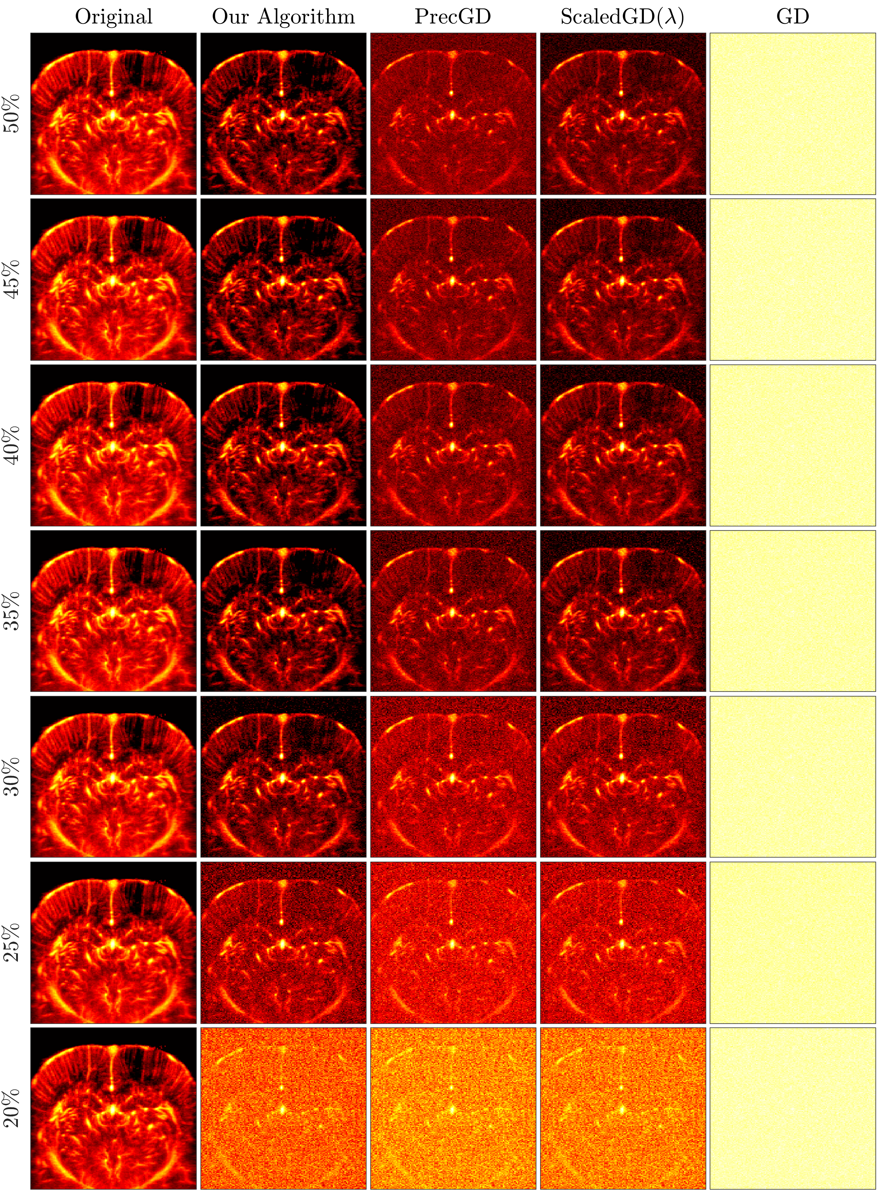
Figure 5: Ultrafast ultrasound image recovery under different downsampling rate. We recover the ultrasound image in Figure 1 under 7 downsampling rates: 50%, 45%, 40%, 35%, 30%, 25% and 20%. The ultrasound images are shown using power Doppler [1]. Column 1: original image. Column 2: image recovered from our algorithm (2). Column 3: image recovered from ScaledGD$(\lambda)$. Column 4: image recovered from PrecGD. Column 5: image recovered from GD.

References

- [1] Jeremy Bercoff, Gabriel Montaldo, Thanasis Loupas, David Savery, Fabien Mézière, Mathias Fink, and Mickael Tanter. Ultrafast compound doppler imaging: Providing full blood flow characterization. IEEE transactions on ultrasonics, ferroelectrics, and frequency control, 58(1):134–147, 2011.
- [2] Srinadh Bhojanapalli, Anastasios Kyrillidis, and Sujay Sanghavi. Dropping convexity for faster semi-definite optimization. In Conference on Learning Theory, pages 530–582. PMLR, 2016.
- [3] Emmanuel J Candes. The restricted isometry property and its implications for compressed sensing. Comptes rendus mathematique, 346(9-10):589–592, 2008.
- [4] Emmanuel J Candès, Xiaodong Li, Yi Ma, and John Wright. Robust principal component analysis? Journal of the ACM (JACM), 58(3):1–37, 2011.
- [5] Emmanuel J Candes, Xiaodong Li, and Mahdi Soltanolkotabi. Phase retrieval via wirtinger flow: Theory and algorithms. IEEE Transactions on Information Theory, 61(4):1985–2007, 2015.
- [6] Emmanuel J Candes and Yaniv Plan. Matrix completion with noise. Proceedings of the IEEE, 98(6):925–936, 2010.
- [7] Emmanuel J Candes and Yaniv Plan. Tight oracle inequalities for low-rank matrix recovery from a minimal number of noisy random measurements. IEEE Transactions on Information Theory, 57(4):2342–2359, 2011.
- [8] Emmanuel J Candès and Benjamin Recht. Exact matrix completion via convex optimization. Foundations of Computational mathematics, 9(6):717–772, 2009.
- [9] Emmanuel J Candes, Thomas Strohmer, and Vladislav Voroninski. Phaselift: Exact and stable signal recovery from magnitude measurements via convex programming. Communications on Pure and Applied Mathematics, 66(8):1241–1274, 2013.
- [10] Emmanuel J Candès and Terence Tao. The power of convex relaxation: Near-optimal matrix completion. IEEE Transactions on Information Theory, 56(5):2053–2080, 2010.
- [11] Gavin C Cawley. Leave-one-out cross-validation based model selection criteria for weighted ls-svms. In The 2006 IEEE international joint conference on neural network proceedings, pages 1661–1668. IEEE, 2006.
- [12] Yudong Chen and Martin J Wainwright. Fast low-rank estimation by projected gradient descent: General statistical and algorithmic guarantees. arXiv preprint arXiv:1509.03025, 2015.
- [13] David Roxbee Cox and David Victor Hinkley. Theoretical statistics. CRC Press, 1979.
- [14] Ernesto De Vito, Andrea Caponnetto, and Lorenzo Rosasco. Model selection for regularized least-squares algorithm in learning theory. Foundations of Computational Mathematics, 5(1):59–85, 2005.
- [15] Bradley Efron and Robert J Tibshirani. An introduction to the bootstrap. CRC press, 1994.
- [16] Maryam Fazel, E Candes, Benjamin Recht, and P Parrilo. Compressed sensing and robust recovery of low rank matrices. In 2008 42nd Asilomar Conference on Signals, Systems and Computers, pages 1043–1047. IEEE, 2008.
- [17] Wendell H Fleming and Raymond W Rishel. Deterministic and stochastic optimal control, volume 1. Springer Science & Business Media, 2012.
- [18] Phillip I Good. Resampling methods. Springer, 2006.
- [19] David Gross, Yi-Kai Liu, Steven T Flammia, Stephen Becker, and Jens Eisert. Quantum state tomography via compressed sensing. Physical review letters, 105(15):150401, 2010.
- [20] Erich L Lehmann and George Casella. Theory of point estimation. Springer Science & Business Media, 2006.
- [21] Jianhao Ma and Salar Fattahi. Implicit regularization of sub-gradient method in robust matrix recovery: Don’t be afraid of outliers. arXiv preprint arXiv:2102.02969, 2021.
- [22] Yurii Nesterov et al. Lectures on convex optimization, volume 137. Springer, 2018.
- [23] Benjamin Recht, Maryam Fazel, and Pablo A Parrilo. Guaranteed minimum-rank solutions of linear matrix equations via nuclear norm minimization. SIAM review, 52(3):471–501, 2010.
- [24] Mickael Tanter and Mathias Fink. Ultrafast imaging in biomedical ultrasound. IEEE transactions on ultrasonics, ferroelectrics, and frequency control, 61(1):102–119, 2014.
- [25] Tony Thomas, Athira P Vijayaraghavan, and Sabu Emmanuel. Machine learning approaches in cyber security analytics. Springer, 2020.
- [26] Tian Tong, Cong Ma, and Yuejie Chi. Accelerating ill-conditioned low-rank matrix estimation via scaled gradient descent. arXiv preprint arXiv:2005.08898, 2020.
- [27] Stephen Tu, Ross Boczar, Max Simchowitz, Mahdi Soltanolkotabi, and Ben Recht. Low-rank solutions of linear matrix equations via procrustes flow. In International Conference on Machine Learning, pages 964–973. PMLR, 2016.
- [28] Xingyu Xu, Yandi Shen, Yuejie Chi, and Cong Ma. The power of preconditioning in overparameterized low-rank matrix sensing. arXiv preprint arXiv:2302.01186, 2023.
- [29] Jialun Zhang, Salar Fattahi, and Richard Y Zhang. Preconditioned gradient descent for over-parameterized nonconvex matrix factorization. Advances in Neural Information Processing Systems, 34:5985–5996, 2021.
- [30] Qinqing Zheng and John Lafferty. A convergent gradient descent algorithm for rank minimization and semidefinite programming from random linear measurements. arXiv preprint arXiv:1506.06081, 2015.
- [31] Jiacheng Zhuo, Jeongyeol Kwon, Nhat Ho, and Constantine Caramanis. On the computational and statistical complexity of over-parameterized matrix sensing. arXiv preprint arXiv:2102.02756, 2021.