To Collide or Not to Collide - Exploiting Passive Deformable Quadrotors for Contact-Rich Tasks

Abstract

With an increase in aerial vehicle applications, passive deformable quadrotors are getting significant attention in the research community due to their potential to perform physical interaction tasks. Such quadrotors are capable of undergoing collisions, both planned and unplanned, which are harnessed to induce deformation and retain stability by dissipating collision energies. In this article, we utilize one such passive deforming quadrotor, XPLORER, to complete various contact-rich tasks by exploiting its compliant chassis via various impact-aware planning and control algorithms. At the core of these algorithms is a novel external wrench estimation technique developed specifically for the unique multi-linked structure of XPLORER’s chassis. The external wrench information is then employed for designing interaction controllers to obtain three additional flight modes: static-wrench application, disturbance rejection and yielding to the disturbance. These modes are then incorporated into a novel online exploration scheme to enable navigation in unknown flight spaces with only tactile feedback and generate a map of the environment without requiring additional sensors. Experiments show the efficacy of this scheme to generate maps of the previously unexplored flight space with an accuracy of 96.72$\%$. Finally, we develop a novel collision-aware trajectory planner (CATAAN) to generate minimum time maneuvers for waypoint tracking by integrating collision-induced state jumps for both elastic and inelastic cases. We experimentally validate that minimum time trajectories can be obtained with CATAAN leading to a 40.38$\%$ reduction of settling time accompanied by improved tracking performance of a root mean squared error in position within 0.5cm as compared to 3cm of conventional methods.

I Introduction

Unmanned aerial vehicles (UAVs) have seen their missions expanding from surveillance to aerial manipulation and physical interaction tasks such as pick and place, grasping, perching, and pushing/pulling [1, 2, 3]. Conventional methods try to accomplish these missions by augmenting UAVs with additional protective gears, graspers, and manipulators to perform the various tasks, coupled with appropriate task-specific control algorithms [4, 5, 6]. While extensive research with such augmented platforms have shown great promise, researchers has also discovered that reconfigurability and mechanical compliance of a UAV chassis can enhance endurance, beget versatility, improve flight efficiency, and enable safe interaction, all at once [7]. Accordingly, various morphing quadrotors have been designed and evaluated for achieving folding, multi-media locomotion and grasping [8, 9, 10].

A majority of such morphing UAVs, however, have active actuation mechanisms for initiating a change in their morphology, classified as $active$ morphing aerial vehicle. In contrast, when the aerial vehicle reacts to external physical forces and undergoes a change in morphology, we call it a passive morphing aerial vehicle [11]. For such vehicles, collision energies are harnessed to initiate deformation using various materials and structures such as springs, foldable origami, and inflatable textiles leading to fast recovery post collisions [12, 13, 14, 15]. This article aims at developing algorithm frameworks for such collision-resilient quadrotors to perform aerial-physical interaction tasks in real-world scenarios.

I-A Related Literature

Critical to any robot-environment physical interaction tasks is the external wrench estimation algorithm which is used to design the interaction controllers [16]. Accordingly, external wrench estimation and interaction control have been extensively investigated in the context of aerial robots and aerial manipulation [17, 18, 19]. One goal of this article is to tailor these concepts for implementation on passive deforming quadrotors to push objects as well as explore and map the environments. Furthermore, due to the collision-resilient feature, this articles aims at leveraging collisions to demonstrate collision-inclusive maneuvers and agile flight behaviors, such as reaching a given target location in minimum time. A brief overview of related work on wrench estimation, contact-based inspection, contact-based/collision-inclusive navigation, and map generation is given in the sections below.

I-A1 External Wrench Estimation

There are generally two approaches for estimating the external wrenches: the first method is to augment the aerial vehicle with sensors such as the force-torque sensors and the second method is to estimate the wrench using onboard sensors. The first method increases the total weight of the aerial vehicle platform and adversely affects flight time [20, 21]. For the second method, researchers have developed algorithms based on momentum-based [22, 23] and acceleration-based [18, 24] wrench estimators which rely on only the available onboard sensors such as inertial measurement units (IMUs). To improve the estimation in presence of sensor noise, a Kalman-filter based approach for wrench estimation was proposed in [25]. Authors of [26] presented significantly more accurate wrench estimates by combining the momentum-based and acceleration-based approaches. For this work, we aim at modifying the acceleration-based wrench estimation algorithm to account for the deformation in the chassis and utilize the proprioceptive information about the vehicle’s current morphology to generate an accurate wrench.

I-A2 Wrench Application and Inspection

Contact-based tasks are recently being pursued with UAVs, such as non-destructive testing, vibration analysis and leak identification which require a desired wrench to be applied onto a surface in an attempt to reduce safety risks to human workers [27, 28]. Successful applications are demonstrated in [29, 30, 31] where the researchers employ conventional rigid multirotor UAVs augmented with external protective gears or end-effectors for performing these contact-rich tasks. One drawback of employing a rigid chassis is that the contact is non-smooth which necessitates a hybrid control law for traversing on the external surface [32, 33]. In this context, we propose to employ soft deformable quadrotors to establish smooth contacts and simplify the contact laws [34].

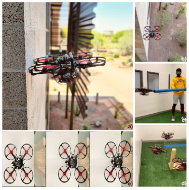
Figure 1: An overview of XPLORER performing various aerial-physical interaction tasks. (a) & (b) Overall vision of this work for deployment in outdoor surveillance missions. (c) Safe interaction policies implemented to enable aerial-human interaction, (d) Collision-inclusive motion planning with the proposed CATAAN algorithm, and (e) A sequence of slow-motion snapshots to highlight the deformation of XPLORER’s chassis for establishing smooth contacts.

I-A3 Contact-based Navigation

The collision-resilient designs hold a strong potential for a paradigm shift from obstacle detection for localization and mapping [35, 36, 37, 38, 39] to tactile-based exploration schemes, also called contact-based navigation. This also is an effective way to reduce weight from the additional sensors that can adversely affect flight time. Contact-based navigation has been successfully implemented by researchers for various applications. Tactile-sensors[40, 41] or inertial measurement units (IMUs) can be successfully used to detect collisions in this case [42, 43, 26]. Then, the motion planner can replan online trajectories by considering these obstacles. A contact-based navigation planner was proposed in [44] consisting of two modes, sliding and flying cartwheel. The drone switches to the cartwheel motion when there are no feasible trajectory for sliding mode or if the drone gets stuck to some map inconsistencies. The authors do state that the flying cartwheel mode has the risk of high collision forces and demanding for robust state estimation. Authors of [41] utilized vision systems to navigate manhole-sized tubes along with flaps to sense contacts. In [45], authors used point cloud information of the environment to compute the trajectory for navigation. In [46] collisions were exploited for path planning using sampling-based methods. The common factor among all these works is that complete knowledge of the map of the environment is known a-priori and they utilize it to compute the trajectory. Navigation in an unknown environment is still nascent and remains an open problem. In [40], the authors proposed a random exploration algorithm, where the vehicle behaves like a bee and starts moving in the direction away from the obstacle. One limitation of this methodology is that with random exploration the coverage rate is not optimal and it is difficult to reproduce the results. It is to be noted that existing work has not leveraged deformable designs to improve flight agility and achieve minimum flight time maneuvers which is one of the goals of our work.

I-A4 Mapping

Exploration and mapping of an environment are synergistic actions and foundations for simultaneous localization and mapping (SLAM). This map generated can be used for trajectory generation by the same vehicle or for other autonomous vehicles. Conventionally, mapping an environment is performed by using cameras and Structure from Motion (SfM) technique [7]. SfM is the process of recreating a 3D structure from a series of images captured from different angles. Authors of [47] proposed an algorithm that used data from Light Detection And Ranging (LiDAR) and a stereo camera to generate a high-resolution map of the environment. As research progressed, real-time map generation was achieved using SLAM algorithms. [48, 49] used a monocular camera to carry out feature recognition and extraction to generate the map and also to localize the drone in the map. Similarly, SLAM was implemented using a 2-axis LiDAR as shown in [50]. Research carried out in [51] used the combination of cameras, LiDAR, IMU, and encoders to generate a highly precise map of the environment. Another novel map generation methodology was presented in [26] where collision detection and localization were used to insert obstacle blocks into the point cloud map. However, the inserted block dimension is constant and does not accurately represent the dimensions of the obstacle, leading to limited online applications.

I-B Contributions of Present Work

Existing work on mechanically compliant quadrotors focuses on improving collision resilience [11, 52]; they have not been investigated to perform contact-based inspection which requires the UAV to maintain continuous contact with the desired object [53, 14]. Our previous work introduces various mechanical designs to obtain 2D and 3D collision resilience which looks beyond collision resilience and proposes harnessing the collision energies to undergo deformation for squeeze-and-fly and perching tasks [12, 54]. Furthermore, in [14], we proposed a recovery controller to stabilize the vehicle after collision by establishing that the post-collision velocities for the passive deformable quadrotors are low and hence the pre-collision velocity can be used to generate a desired position setpoint in the opposite direction of approach. Researchers in [13] presented another collision-tolerant vehicle with a recovery controller which leveraged collision characterization to generate a desired position setpoint. Controlled collision was further exploited in [55] to demonstrate narrow gap traversal with a soft foldable frame. However, this article aims to explore further benefits of these novel passive reconfigurable quadrotors for performing exhaustive contact-rich tasks such as exploration, navigation and mapping. The advantage of having a deformable chassis makes passive reconfigurable UAVs as ideal candidates to make, break or sustain contacts and apply desired contact forces without exhaustive hybrid control strategies. Furthermore, since collision energies are absorbed by frame deformation, the dynamics when the state crosses this collision plane can be modeled as a hybrid automaton and employed to derive minimum time trajectories, even faster than those obtained from the classical bang-bang control [56]. We derive the necessary conditions for minimal flight time to reach a destination by allowing the UAV to intentionally collide on objects, and show via experiments how shortest-time trajectories can be obtained with our novel collision-inclusive trajectory planner.

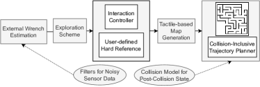
Figure 2: An overview of the contributions from this article. The rectangular shaded blocks show the proposed algorithms and the elliptical blocks show the additional modules necessary for the implementation of the algorithms.

The main contributions of the article are shown in Fig. 2 and described as follows:

1. We propose an external wrench estimation algorithm for a deformable, multi-link aerial vehicle.

2. An exploration algorithm is developed that only relies on tactile feedback and external wrench to detect objects and navigate through unknown environments.

3. A novel map generation scheme is proposed for unknown environments using the wrench estimation feedback in addition to position and orientation of the vehicle.

4. A data-driven collision model is fitted using a neural network to accurately predict the post-collision state for a given pre-collision state and angle of incidence to the collision plane

5. We develop and validate a collision inclusive motion planner to exploit collisions and generate minimum-time trajectories to the goal location within the map.

To the best of the authors’ knowledge, this is the first comprehensive work that successfully demonstrates the benefits of passive reconfigurable quadrotors for contact-rich tasks such as exploration, tactile-feedback based map generation and collision-inclusive minimum-time trajectories.

The rest of the paper is organized as follows: Section II overviews of the design and low-level control of the aerial vehicle, XPLORER. The novel external wrench estimation algorithm developed for XPLORER’s unique design is introduced in Section III. Section IV describes the exploration and tactile-based mapping scheme. Section V details the novel collision-inclusive trajectory planner and Section VI presents all the results for the proposed algorithms in real-world implementations. Finally Section VII concludes the article and discusses potential future work.

II System Description

A brief overview of the system, XPLORER, is given in the following subsections for the design and the low-level control.

II-A Design of XPLORER

In this work, we use a modified version of the passive foldable aerial robot, SQUEEZE, presented in our previous work [12]. Built on the similar idea, XPLORER (shown in Fig. 1) also has four deformable arms as part of its morphing chassis, but it does not retain the complete arm rotation to 90^o like its predecessor. The springs chosen for the current version are also stiffer than our previous design to ensure that the collision-induced deformation is induced in a smaller range. The free rotation is limited to 30^o due to the preferred in-plane placement of the arms unlike in SQUEEZE. This design choice was made for two specific reasons, with the first being that we wanted to lower the height of the center of mass (CoM) from our previous design to prevent toppling when making contacts with the environment. This is shown in Fig. 1(e) where the deformation of the chassis easily allows large forces around 1N to be exerted on the environment without pitching into the wall unlike the rigid conventional chassis. Secondly, we need to ensure that the vehicle will not get stuck in corner cases during exploration and hence redesigned the propeller guards, so a maximum of $30^{o}$ of free rotation was obtained as a result. Accordingly, since the scope of this article is to explore contact-based tasks and not to showcase squeeze and fly abilities, we limit the linear velocities to 4 m/s such that collisions which result in more than $30^{o}$ arm deformation are avoided. Each arm has an sensor attached to it to measure its relative orientation with respect to the body, which will be later used for external wrench estimation.

II-B Control Framework

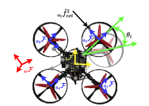
Figure 4: A visualization of the frames used to compute the net external wrench. The collision force (${}_{a_{2}}\hat{f}_{ext}^{2}$) is identified as a vector in the arm frame ${}_{a_{i}}\mathcal{F}$. The net wrench is then obtained using (4).

In this section we describe the complete control framework for XPLORER. The control block diagram is shown in Fig. 3. The coordinate frame definitions and symbols used are described in Table I and are shown in Fig. 4. Each arm frame, ${}_{a_{i}}\mathcal{F}$, is located at a distance $r_{i}$ from the geometric center ($\mathcal{O}_{w}$) of the frame. The body frame, ${}_{b}\mathcal{F}$ denotes the body-fixed frame $\{b_{1},b_{2},b_{3}\}$ located at $\mathcal{O}_{w}$ while ${}_{w}\mathcal{F}$ denotes the inertial frame $\{e_{1},e_{2},e_{3}\}$.

The complete rigid body dynamics of XPLORER can be written as

$$\centering\boldsymbol{\dot{x}}\@add@centering =\boldsymbol{v}$$

$$m\boldsymbol{\dot{v}} =mg\boldsymbol{e}_{3}-f\boldsymbol{R}\boldsymbol{e}_{3}+\boldsymbol{\delta}_{f}$$ (1a)

$$\boldsymbol{\dot{R}} =\boldsymbol{R}\hat{\boldsymbol{\Omega}}$$

$$\boldsymbol{H}\dot{\boldsymbol{\Omega}} -[\boldsymbol{H}\boldsymbol{\Omega}]_{\times}\boldsymbol{\Omega}=\boldsymbol{\tau}+\boldsymbol{\delta}_{\tau}$$ (1b)

where $m$ denotes the mass of the vehicle, $[\boldsymbol{x,v,R,\Omega}]^{T}$ denote the position, translational velocity, rotation from body frame to world frame (i.e $\boldsymbol{R}:=~{}{{}_{b}}^{w}\boldsymbol{R}$) and angular velocity respectively of the system. The terms $\boldsymbol{\delta}_{f}\in\mathbb{R}^{3}$ and $\boldsymbol{\delta}_{\tau}\in\mathbb{R}^{3}$ denote the external wrenches applied on the system assumed in this work as lumped disturbances. The hat map $\hat{\cdot}:\mathbb{R}^{3}\xrightarrow{}\mathsf{SO(3)}$ is a symmetric matrix operator defined by the condition that $\boldsymbol{\hat{x}y=x\times y}~{}\forall~{}\boldsymbol{x,y}\in\mathbb{R}^{3}$ and $[.]_{\times}$ is the skew symmetric cross product matrix. The rest of nomenclature is given in Table I.

TABLE I: Symbols and Definitions

Symbol	Definition
$\boldsymbol{m}$	mass of the system
$\boldsymbol{H}$	moment of inertia of system
$\mathcal{O}_{w}$	vehicle geometric center
${}_{w}\mathcal{F}=\{e_{1},~{}e_{2},~{}e_{3}\}$	inertial frame
${}_{b}\mathcal{F}=\{b_{1},~{}b_{2},~{}b_{3}\}$	body fixed frame, with $\mathcal{O}_{w}$ fixed at the geometric centre of the frame
${}_{a_{i}}\mathcal{F}=\{a_{1}^{i},~{}a_{2}^{i},~{}a_{3}^{i}\}$	$i^{th}$ arm frame for estimating the external force on $i^{th}$ arm
$[\boldsymbol{\delta_{f}}~{}\boldsymbol{\delta_{\tau}}]^{T}$	true external wrench
$[\hat{\boldsymbol{\delta_{f}}}~{}\hat{\boldsymbol{\delta_{\tau}}}]^{T}$	estimated external wrench
$[_{b}\hat{\boldsymbol{\delta_{f}}}~{}_{b}\hat{\boldsymbol{\delta_{\tau}}}]^{T}$	estimated external wrench in body frame
$\boldsymbol{C}_{n}$	contact normal to the obstacle
$\lambda$	current move direction of the vehicle
$d_{step}$	distance to move for each step
$\dot{\psi_{0}}$	yaw rate threshold
$\dot{\psi_{c}}$	tactile turning yaw rate
$\boldsymbol{\delta}_{0}$	force threshold for exploration & tactile-traversal
${{\boldsymbol{\delta_{\psi}}}}_{0}$	force threshold for tactile-turning
$f_{des}$	force to be applied on the obstacle
$\boldsymbol{\delta}_{map}$	force threshold for mapping

A cascaded P-PID control law is employed for both the position and attitude loops of the low-level controller for XPLORER as shown in Fig. 3 with the errors defined on position and quaternion space respectively. We take advantage of the inherent robustness of the P-PID control structure to obtain good tracking performance in the presence of model uncertainties such as the placement of the arms which can affect the conversion of the control inputs to individual motor inputs. However, as mentioned in Section II-A, the deformation doesn’t last very long due to the spring action and therefore a P-PID structure works well for all our experiments. The design of robust controllers to account for disturbances and model uncertainties is beyond the scope of this work and planned in a future study [57].

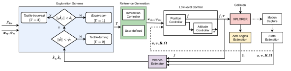
Figure 3: Complete block diagram for an autonomous exploration task with XPLORER. Collisions are characterized by the external wrench shown by the purple shaded block. This value is used to decide the state of exploration ($\Gamma$) as shown by the state-machine in the blue shaded block. The value of $\Gamma$ is then used to generate a suitable reference for position ($x_{des}$) and yaw ($\psi_{des}$) by either using the interaction controller to reshape the setpoint specified by the user ($x_{sp}$, $\psi_{sp}$) using $F_{des}$ or bypassing the reshaping process as shown by the green colored block. Finally these references are published to the low-level P-PID tracking controller of the vehicle. The yellow shaded block denotes the arm-angle estimation critical to the proposed external wrench estimation algorithm.

III External Wrench Estimation and Interaction Control

This section describes the novel external wrench estimation algorithm developed and the corresponding interaction controller, an admittance controller [26], designed by using the wrench estimates.

III-A External Wrench Estimation

Since the aerial vehicle XPLORER is composed of multiple rigid bodies, the wrench estimate using the acceleration method only on the center of mass (CoM) is an inaccurate representation of the actual wrench acting on the body. However, by estimating the wrench applied on each arm, we can estimate the net external wrench by combining the acceleration-based methods on the CoM with the estimated wrench on the arm.

The frames used for calculating the wrench is shown in Fig. 4. The yellow frame denotes the body frame of the vehicle at any instant, the red frame denotes the world inertial frame and the blue frames denote the arm frame for four arms respectively.

In this work, we are primarily interested in estimating the net wrench acting on XPLORER and therefore assume that the external wrench $[\boldsymbol{\delta_{f}}~{}\boldsymbol{\delta_{\tau}}]^{T}$ is in a lumped form, as shown in (1a) and (1b). This implies that we do not isolate aerodynamic wrench and collision wrench for the scope of this work. However, our future work will incorporate precise aerodynamic models to allow individual identification of these two types of external wrenches. Moreover, even though the wrench acts on the propeller guard, we assume that it acts at the origin of the arm frame, normal to the arm as shown by ${{}_{a_{3}}}{\hat{f}_{{ext}_{i}}}$ in Fig. 4. This is due to only $\pm$0.5cm difference in the possible locations of wrench application on the propeller guard, and we do not account for the exact location.

III-B Arm Wrench

We begin by estimating the external force on each arm by employing the acceleration-based method. Due to the torsional springs employed at the arm hinge, the arm dynamics can be written as:

$$\ddot{\theta}_{i}+k\dot{\theta}_{i}+b\theta_{i}=\hat{\delta}_{f_{a_{i}}}.$$ (2)

Since the arm angle information is obtained from the IMU sensor, numerical differentiation of this data can be very noisy, so we employ a first order low-pass filter to estimate the force on the $i^{th}$ arm by

$${}_{a_{i}}{\dot{\hat{\delta}}}_{f_{a}} =K_{I}(_{a_{i}}\delta_{f_{a}}-{{}_{a_{i}}}\hat{\delta}_{f_{a}})$$ (3)

where ${}_{a_{i}}\hat{\delta}_{f_{a}}$ denotes the wrench obtained in the $i^{th}$ arm frame, $K_{I}$ denotes the filter gain and the ${}_{a_{i}}\delta_{f_{a}}$ denotes the true wrench.

III-C Wrench Estimate at CoM

Next, following [26], the wrench information at the CoM can be directly estimated from the acceleration measurement of the vehicle. Rearranging (1a) and (1b, we obtain

$$\hat{\boldsymbol{\delta}}_{f_{CoM}} =m\boldsymbol{\dot{v}}-mg\boldsymbol{e}_{3}+f\boldsymbol{R}$$ (4)

$$\hat{\boldsymbol{\delta}}_{\tau_{CoM}} =\boldsymbol{H}\dot{\boldsymbol{\Omega}}-[\boldsymbol{H}\boldsymbol{\Omega}]_{\times}\boldsymbol{\Omega}-\boldsymbol{\tau}$$

We again filter the obtained acceleration to calculate the external wrench. A median with a low pass filter is used to get a smooth approximation of the acceleration and the control input.

III-D Net Wrench on XPLORER

With the wrench estimate on each arm, the external arm wrench in the inertial frame can be written as:

$${}_{w}\hat{\boldsymbol{\delta}}_{f_{a_{i}}}=_{b}^{w}\boldsymbol{R}~{}_{a_{i}}^{b}\boldsymbol{R}~{}_{a_{i}}\hat{\boldsymbol{\delta}}_{f_{a_{i}}}$$ (5)

where ${}_{b}^{w}\boldsymbol{R}$ denotes the rotation from the body frame to the inertial frame and ${}_{a_{i}}^{b}\boldsymbol{R}$ denotes rotation from the arm frame to the body frame as given by (6) below

$$_{a_{i}}^{b}\boldsymbol{R}=\begin{bmatrix}\cos\theta_{i}&-\sin\theta_{i}\\ \sin\theta_{i}&\cos\theta_{i}\end{bmatrix}$$ (6)

We can now estimate the net external wrench on XPLORER by combining (3) and (4):

$$\hat{\boldsymbol{\delta}}_{f} ={\hat{\delta}}_{f_{CoM}}+\sum_{i=1}^{4}{{}_{w}}{\hat{\boldsymbol{\delta}}}_{f_{a_{i}}}$$ (7)

$$\hat{\boldsymbol{\delta}}_{{\tau}} ={\hat{\boldsymbol{\delta}}}_{{{{\tau}}_{CoM}}}+\sum_{i=1}^{4}{{}_{w}}{\hat{\boldsymbol{\delta}}}_{{{{\tau}}_{a_{i}}}}$$

III-E Interaction Control

In this section we design an admittance controller that reshapes the reference trajectory and yaw setpoint to maintain a desired force $f_{des}$. The estimated wrench can be used for two different modes depending on what we want XPLORER to perform. The first mode is that we can employ the external wrench to exert a specific force on the surface and in the second mode, it can be used to steer clear of objects when a contact is detected. For both these cases, an admittance controller was designed to maintain a desired interaction force.

To achieve this goal, we employ standard admittance control strategies [26] and model the desired response as a virtual second order dynamics:

$$\begin{bmatrix}m_{v}&0\\ \boldsymbol{0}_{3\times 3}&I_{v,z}\end{bmatrix}\begin{bmatrix}\ddot{r}_{d}\\ \ddot{\psi}_{d}\end{bmatrix}+\boldsymbol{D}\begin{bmatrix}\dot{r}_{d}\\ \dot{\psi}_{d}\end{bmatrix}+\boldsymbol{K}\begin{bmatrix}r_{d}-r_{d}^{*}\\ \psi_{d}-\psi_{d}^{*}\end{bmatrix}=\begin{bmatrix}\hat{\boldsymbol{\delta}}_{{{}_{f}}}\\ {\boldsymbol{\hat{\delta}}}_{{\tau}_{e,z}}\end{bmatrix},$$ (8)

where $m_{v}>0$ and $I_{v,z}>0$ are the virtual mass and inertia, $D_{v}\in\mathbb{R}^{4\times 4}$ is the positive definite diagonal virtual damping gain, $\boldsymbol{K}_{v}\in\mathbb{R}^{4\times 4}$ is the positive diagonal virtual spring gain, $r_{d}^{*}$ and $\psi_{d}^{*}$ are the optimal desired setpoints of position and yaw, respectively. $\hat{f}_{ext}$ is the estimated external force, and $\hat{\tau}_{e,z}$ is the estimated external torque about the $z$-axis (external yaw torque).

IV Contact-based Exploration and Mapping

This following two subsections describe the complete autonomous exploration and mapping algorithms respectively, developed uniquely for XPLORER by employing the external wrench estimation technique proposed in Section (III-A) with a suitable reference generation scheme. The reference generation scheme alternates between using a predefined set-point or a reshaped version of it by using the interaction controller from Section III-E as further discussed below.

IV-A Contact-based Exploration

This section presents a navigation algorithm that allows XPLORER to explore its surrounding environment. The algorithm uses an explore-and-exploit strategy, taking advantage of the collision-resilient design and the admittance controller to perform tactile-based navigation. This is achieved through a finite state machine shown in Fig. 3, utilizing, $\hat{\boldsymbol{\delta_{f}}}\in\mathbb{R}^{3}$, representing the force estimate in the inertial frame and yaw rate, $\dot{\psi}\in\mathbb{R}$, as inputs to generate the reference trajectory, $[x_{sp}~{}\psi_{sp}]^{T}$. The workflow of the algorithm is discussed below.

First, the external wrench needs to be transformed into the body frame using the equation below

$$_{b}\hat{\boldsymbol{\delta_{f}}}=_{w}^{b}\boldsymbol{R}\hat{\boldsymbol{\delta}}_{f},$$ (9)

where ${}_{w}^{b}\boldsymbol{R}$ denotes the rotation matrix from the inertial frame to the body frame.

The state machine comprises three primary states: Exploration, Tactile-turning and Tactile-traversal corresponding to $\Gamma\in\{1,2,3\}$ respectively. Except for Tactile-turning, the yaw admittance controller is used to generate yaw setpoints and enable XPLORER to conform to the obstacle’s surface. In obstacle-free flight, XPLORER experiences negligible yaw torques and external forces. We choose this as the trigger condition for entering $\Gamma=1$, i.e. the exploration state. In this state, the vehicle continues to fly forward in space until it encounters an object in its flight path. If $|\dot{\psi}|<\dot{\psi}_{0}$ and $|_{b}\hat{\boldsymbol{\delta_{f}}}|<{{\boldsymbol{\delta}}}_{0}$, XPLORER switches to the Exploration state as depicted in Alg. 1 and generates trajectory setpoints along the body x-axis.

At any given time, the state machine continuously checks $\dot{\psi}$ to detect any yawing around a point. The yawing can happen when the vehicle is sliding across an edge of an object by exerting a desired force and at the corner it releases the contact. Since the yaw generation is in admittance, this phenomenon causes the yaw rate to peak instantaneously due to the sudden release. Accordingly we check if $|\dot{\psi}|>\dot{\psi}_{0}$, where $\dot{\psi}_{0}$ is the threshold for triggering the Tactile-turning state shown in Alg. 2. In this state, a controlled yaw is generated at a rate of $\dot{\psi}_{c}$ in the same direction as XPLORER’s yaw until $|_{b}\hat{\boldsymbol{\delta}}_{f}|>{{\boldsymbol{\delta_{\psi}}}}_{0}$ about either axis. ${{\boldsymbol{\delta_{\psi}}}}_{0}$ has to be higher than ${{\boldsymbol{\delta}}}_{0}$ because upon switching to Tactile-traversal state the $|_{b}\hat{\boldsymbol{\delta}}_{f}|$ should be greater than the ${{\boldsymbol{\delta}}}_{0}$ to register contact and update the contact $\boldsymbol{C_{n}}\in\mathbb{R}^{4}$, which represents the contact direction in the positive x, negative x, positive y, and negative y directions in the body frame and it is expressed as:

$$\boldsymbol{C_{n}}=[+x,-x,+y,-y]^{T}.$$ (10)

The threshold $\dot{\psi}_{0}$ is chosen to be high enough such that small yaw rates do not trigger the Tactile-turning state. Furthermore, the generated $\psi$ is also limited to 180 degrees to prevent the drone from yawing indefinitely, in this way drone will be able to establish contact with the wall again.

Alg. 3 illustrates the Tactile-traversal state which allows the EXPLORER to traverse obstacles by maintaining contact with obstacle. Upon encountering an obstacle, the vehicle has to move in a direction perpendicular to the obstacle’s surface to continue exploring. To ensure consistency in the exploration path, XPLORER always moves towards the right-hand side of the obstacle’s surface normal.

1

2

Input: $\dot{\psi}\hskip 2.84544pt\&\hskip 2.84544pt_{b}\hat{\boldsymbol{\delta}}_{f}$

Output: $[{x_{sp_{body}}}~{}\psi_{sp}]^{T}$ & $\Gamma$

3

4if $|\dot{\psi}|<\dot{\psi}_{o}\hskip 2.84544pt\&\hskip 2.84544pt|_{b}\hat{\boldsymbol{\delta}}_{f}|<{{{\delta}}}_{0}$ then

5       $X_{sp}(k)=x+d_{step}$
$Y_{sp}(k)=Y_{sp}(k-1)$
$\psi_{sp}=\psi_{des}(\psi)$

6else if $|\dot{\psi}|>\dot{\psi}_{o}$ then

7       $\Gamma=2$

8else

9       $\Gamma=3$

Algorithm 1 Exploration

1

Input: $\dot{\psi}\hskip 2.84544pt\&\hskip 2.84544pt_{b}\hat{\boldsymbol{\delta}}_{f}$

Output: $[{x_{sp_{body}}}~{}\psi_{sp}]^{T}$ & $\Gamma$

2

3if $|\dot{\psi}|>\dot{\psi}_{o}$ & $|_{b}\hat{\boldsymbol{\delta}}_{f}|<{{{\delta_{\psi}}}}_{0}$ then

4      $\boldsymbol{x_{sp}}(k)=\boldsymbol{x_{sp}}(k-1)$
if $\dot{\psi}>\dot{\psi}_{o}$ then

5             $\psi_{sp}(k)=\psi_{sp}(k-1)+\dot{\psi_{c}}dt$

6      else

7             $\psi_{sp}(k)=\psi_{sp}(k-1)-\dot{\psi_{c}}dt$

8      

9else

10       $\Gamma=3$

Algorithm 2 Tactile Turning

1

2

Input: $\dot{\psi}\hskip 2.84544pt\&\hskip 2.84544pt_{b}\hat{\boldsymbol{\delta_{f}}}$

Output: $[{x_{sp_{body}}}~{}\psi_{sp}]^{T}$ & $\Gamma$

3

4

5 Function CollisionNormal():

6       if $\lambda=+Xor-X$ then

7             if ${}_{b}\hat{{\delta_{f}}}_{x}>{{{{\delta}}}_{0}}_{x}$  then

8                   $\boldsymbol{C_{n}}=[1,0,0,0]$

9            else if ${}_{b}\hat{{\delta_{f}}}_{x}<-{{{{\delta}}}_{0}}_{x}$ then

10                   $\boldsymbol{C_{n}}=[0,1,0,0]$

11            

12      else if $\lambda=+Yor-Y$ then

13             if ${}_{b}\hat{{\delta_{f}}}_{y}>{{{{\delta}}}_{0}}_{y}$  then

14                   $\boldsymbol{C_{n}}=[0,0,1,0]$

15            else if ${}_{b}\hat{{\delta_{f}}}_{y}<-{{{{\delta}}}_{0}}_{y}$ then

16                   $\boldsymbol{C_{n}}=[0,0,0,1]$

17            

18      

19      return $\boldsymbol{C_{n}}$

20

21 Function MoveDirection():

22       $\boldsymbol{C_{n}}\leftarrow$ ContactNormal()
if $C_{n}==[1,0,0,0]$ then

23            $\lambda=+Y$

24      else if $C_{n}==[0,1,0,0]$ then

25            $\lambda=-Y$

26      else if $C_{n}==[0,0,1,0]$ then

27            $\lambda=-X$

28      else if $C_{n}==[0,0,0,1]$ then

29            $\lambda=+X$

30      

31      return $\lambda$

32

33 Function TrajectoryGeneration():

34      

35      ${\lambda}\leftarrow$ MoveDirection()
$\psi_{sp}=\psi_{des}(\psi)$
if $\lambda=+X$ then

36             $X_{sp}(k)=x+d_{step}$
$Y_{sp}(k)=Y_{des}(f_{des})$

37      else if $\lambda=-X$ then

38             $X_{sp}(k)=x-d_{step}$
$Y_{sp}(k)=Y_{des}(f_{des})$

39      else if $\lambda=+Y$ then

40             $X_{sp}(k)=X_{des}(f_{des})$
$Y_{sp}(k)=y+d_{step}$

41      else if $\lambda=-Y$ then

42             $X_{sp}(k)=X_{des}(f_{des})$
$Y_{sp}(k)=y-d_{step}$

43      

Algorithm 3 Tactile Traversal

This state is triggered when $|\dot{\psi}|<\dot{\psi}_{o}$ and $|_{b}\hat{\boldsymbol{\delta}}_{f}|>{{\boldsymbol{\delta}}}_{0}$ along any axis. XPLORER continues to move in the previous direction $\mathbf{\lambda}$ until ${{\boldsymbol{\delta}}}_{0}$ is reached and $\boldsymbol{C_{n}}$ is updated. The movement direction $\mathbf{\lambda}$ is updated with positive x, negative x, positive y, and negative y based on which the trajectory is generated. Depending upon the collision direction, the elements of the vector are updated by a binary value. Based on $\boldsymbol{C_{n}}$, $\mathbf{\lambda}$ also gets updated. The latest $\mathbf{\lambda}$ should be normal to the obstacle plane. The interaction controller ensures the vehicle maintains a contact with the obstacle by exerting a force of $f_{des}$. In scenarios where XPLORER encounters obstacles in two directions, $\boldsymbol{C_{n}}$ is updated with the latest collision direction. $\mathbf{\lambda}$ is updated accordingly and the corresponding trajectory is generated.

The trajectory generation is performed in the body frame and then transformed to the inertial frame before being published into the flight controller, as shown below.

$$[x_{sp}~{}y_{sp}]^{T}=_{b}^{w}\boldsymbol{R}[x_{sp_{body}}~{}y_{sp_{body}}]^{T}.$$ (11)

To ensure the setpoints are within $d_{step}$, i.e. the frontier region of the current position of the vehicle, the setpoints are bounded. While exploring, the setpoint for the z-axis is kept constant, as this work focuses on exploring the 2D space. The exploration of the entire 3D space is beyond the scope of this study.

IV-B Contact-based Mapping

The ability to explore the environment by maintaining contact can be used to generate a map of the obstacle. This synthesized map can be used for motion planning by XPLORER or other autonomous robots. The overview of the contact-based mapping framework is depicted in Alg. 4. The algorithm utilizes the ${}_{b}\hat{\boldsymbol{\delta}}_{f}$, the CAD model of XPLORER, and the global pose to generate the obstacle boundary map. We use the Open3D library[58] for processing the point cloud generated.

1

2

Input: $[x,y,z]^{T}\hskip 2.84544pt,\hskip 2.84544pt{\psi}\hskip 2.84544pt,\hskip 2.84544pt_{b}\hat{\boldsymbol{\delta}}_{f}\hskip 2.84544pt,\hskip 2.84544pt\boldsymbol{C_{n}}\hskip 2.84544pt\&\hskip 2.84544pt\lambda$

Output: $Point\hskip 2.84544ptCloud\hskip 2.84544ptData$

3

4if ${}_{b}\hat{\boldsymbol{\delta}}_{f}>\boldsymbol{\delta}_{map}$ then

5       if $\lambda_{prev}\hskip 2.84544pt\neq\hskip 2.84544pt\lambda$  then

6             Add Corner Block to Point Cloud

7      else

8             Add Obstacle to Point Cloud in $\boldsymbol{C_{n}}$ axis

9      

10else

11       Store Point Cloud Data

Algorithm 4 Mapping Framework

Obstacle map generation initializes when ${}_{b}\hat{\boldsymbol{\delta}}_{f}>\boldsymbol{\delta_{map}}$. $\boldsymbol{\delta_{map}}$ is taken to be slightly higher than $f_{des}$. This choice is to ensure mapping is conducted only when there is a firm contact with the obstacle. As an additional condition, the mapping on starts if the drone is flying. The contact normal, $\boldsymbol{C_{n}}$, provides the direction of the obstacle, in which an object of dimension 0.25 m $\times$ 0.08m $\times$ 0.5 m is added to the point cloud, offset by 0.21 m from the position of XPLORER. The offset corresponds to the perpendicular distance from XPLORER’s center to the edge of each side. In corner cases where the move direction, $\lambda$, is not the same as the previous move direction, a constant block is added diagonally with offset of 0.417 m to the point cloud to make it continuous around the corners (shown in Supplementary Video 3). The point cloud is generated at 30 Hz to obtain a high-resolution map of the obstacle. The map is stored as a Polygon File Format (PLY) as per the ASCII format, and it consists of the location of the each point in the point cloud. For this scope of the work the map generation was done on a computer with AMD Ryzen 5 CPU with 16 Gigabytes of RAM, the DDS middleware used in ROS2 enabled offloading the computation from the high-level companion computer to a powerful computer on the same network. The map generation primarily relies on the pose of the drone, which is currently obtained using the motion capture system. We currently employ motion capture system to obtain the drone’s pose, but other state estimation methods like visual-inertial odometry or GPS and IMUs to obtain the pose of the vehicle.

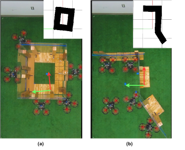
Figure 5: Top view of the experimental setups with the generated maps and overlaid images of XPLORER throughout the experiment. (a) Environment with a closed box-like structure. (b) Environment with concave and convex edges, representing a wall-like structure. Please note that the results for these experiments are shown in the Fig. 8.

V Collision-Aware TrAjectory plAnNer- CATAAN

In this section, we explore the problem of collision-inclusive trajectory planning and demonstrate the performance of the motion planner in 1D. For generating the reference position, we consider a double integrator system dynamics for XPLORER with state-driven jumps and a time-optimal control law is derived for this model. Next, two special cases of this problem are analyzed - collide-to-stop and collide-to-decelerate, which encompasses collisions with passive deformable quadrotors for collisions with varying rebound velocities under different angle of incidence to the collision surface.

Consider the following double integrator dynamics for a continuous-time system with states $x\in\mathbb{R}^{2}$:

$$\dot{x}_{1} =x_{2}$$ (12)

$$\dot{x}_{2} =u$$

It is assumed that the jump pattern is induced by the flow set $\mathcal{C}:=\{x\in\mathbb{R}^{2}\}$ and the jump set which denotes the states where XPLORER undergoes collision and hence has a discontinuity in its state as defined by:

$$\mathcal{D}=\{x\in\mathbb{R}^{2}|x_{1}=a,x_{2}\leq 0\},$$ (13)

where $a$ is the location of object that XPLORER can possibly collide on. Furthermore, let the hybrid system be described by:

$$\dot{x}=Ax+Bu~{}~{}~{}~{}~{}~{}~{}x\in\mathcal{C}$$ (14)

$$x^{+}=Ex~{}~{}~{}~{}~{}~{}~{}~{}~{}~{}~{}~{}x\in\mathcal{D}$$

where $E$ denotes the evolution of the state during the jump.

V-A Time Optimal Control without Collisions

In this section, we briefly present the conventional time-optimal control for a sytem to reach $(0,0)$ from a state $x_{0}$. It is well-known that the solution to the minimum time control problem

$$\min_{u} \int_{0}^{T}dt$$ (15)

is given by the bang-bang control law where the control only takes the values $\{-1,1\}$ and at most one switch is required. More specifically, the trajectories are characterized by the family of the parabolas:

$$\begin{cases}u=+1\\ \begin{cases}x_{1}(t)=+\frac{1}{2}t^{2}+\alpha t+\beta\\ x_{2}(t)=+t+\alpha\end{cases}\\ x_{1}=\frac{1}{2}x_{2}^{2}+\beta-\frac{\alpha^{2}}{2}\end{cases}\begin{cases}u=-1\\ \begin{cases}x_{1}(t)=-\frac{1}{2}t^{2}+\alpha t+\beta\\ x_{2}(t)=-t+\alpha\end{cases}\\ x_{1}=-\frac{1}{2}x_{2}^{2}+\beta-\frac{\alpha^{2}}{2}\end{cases}$$

The switching curve $\Pi$ is defined by:

$$\Pi:=\{x=x_{1}+\frac{1}{2}x_{2}|x_{2}|\}$$

and accordingly we have the disjoint union

$$\mathbb{R}^{2}=S^{-}\cup\Pi\cap S^{+},$$

where $S^{\pm}$ stands for the regions below and above the switching curve $\Pi$.

Furthermore, given the initial condition, the optimal time is given by:

$$t_{0}^{*}(x_{0})=\begin{cases}2\sqrt{\frac{1}{2}x_{2_{0}}^{2}+x_{1_{0}}}+x_{2_{0}},x_{0}\in S^{-}\\ |x_{2_{0}}|,x_{0}\in\Pi\\ 2\sqrt{\frac{1}{2}x_{2_{0}}^{2}-x_{1_{0}}}-x_{2_{0}},x_{0}\in S^{+}\end{cases}$$ (16)

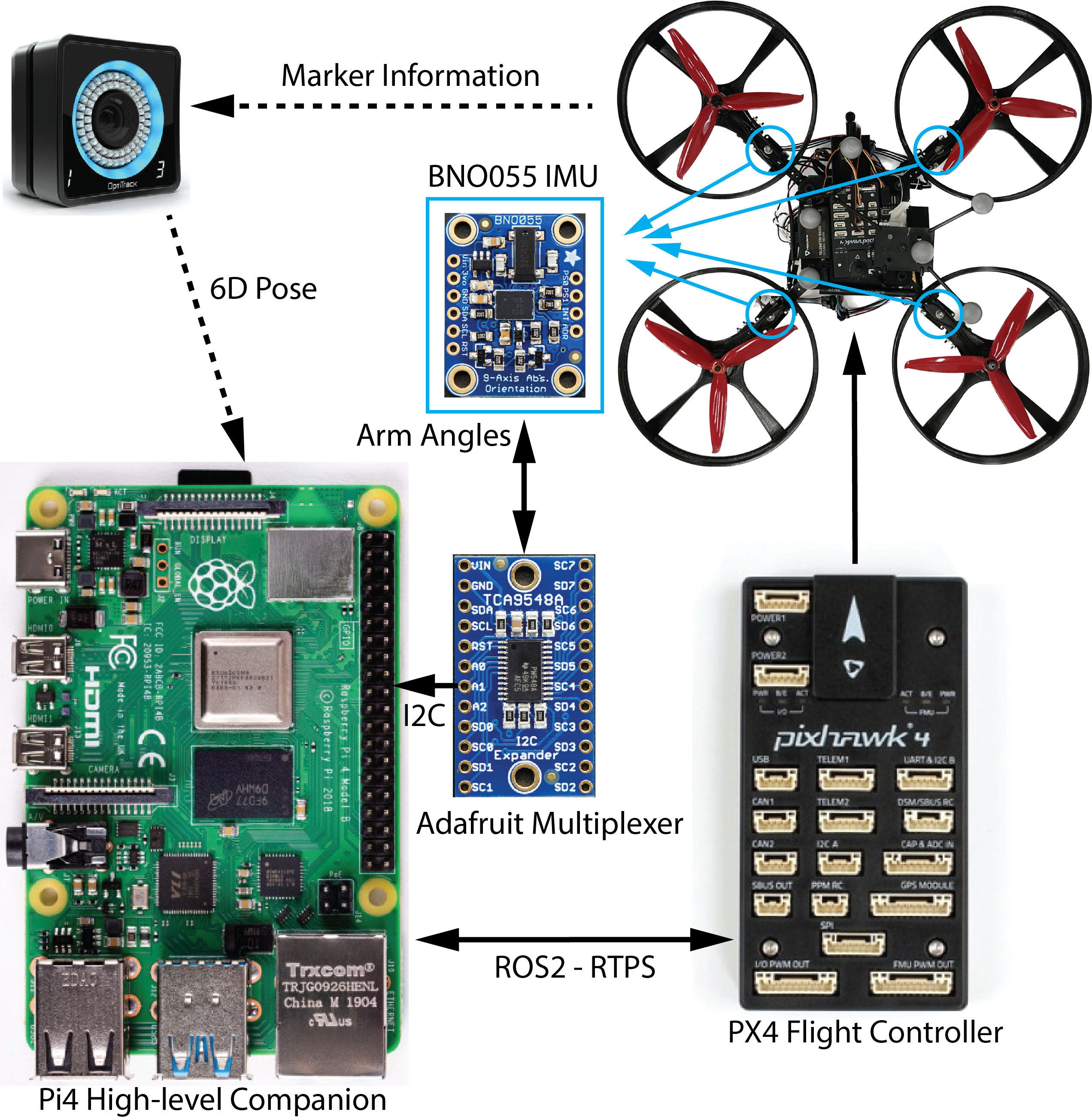
Figure 6: The complete electronics overview for autonomous exploration, map-generation and trajectory tracking missions with XPLORER. IMUs (BNO055) are used to obtain the proprioceptive information about XPLORER’s arm angles. A motion capture system is used to obtain the localization information and a Raspberry Pi4 is employed as the the high-level companion computer.

V-B Time Optimal Control with 1 State Jump due to Collisions

We now extend the analysis to study the case scenarios where collisions induce a state jump in velocity. For this case the, let the jump map $E$ be given by:

$$E=\begin{bmatrix}1&0\\ 0&e\end{bmatrix}$$ (17)

where $e$ stands for the coefficient of post collision velocity as a function of the coefficient of restitution. In this paper, we build a data-driven model to predict the post-collision velocity, as shown in Section VI-E2. This value $e$ can be obtained using a linearization of the collision model. Then any generic point $z$ on the jump set $\mathcal{D}$ can be denoted by $z=(a,\zeta)$ where $a$ denotes the position of the wall and $\zeta$ denotes the pre-collision velocity. The optimal path to $z$ from any given initial point $x_{0}$ are given by the two branches of parabolas with a switching curve passing through $z$ as [56];

$$\Phi(\zeta)=\{x:\frac{1}{2}(x_{2}+\zeta)|x_{2}-\zeta|-a+x_{1}\}$$

We can again decompose the state space as:

$$\mathbb{R}^{2}=\Psi^{-}\cup\Phi\cap\Psi^{+},$$

where $\Psi^{\pm}$ is similarly defined as the regions below and above the switching curve $\Phi$. The optimal time taken to reach $z$ from $x_{0}$ can then be written as:

$$\tau(x_{0},\zeta)=\begin{cases}\Bigg{|}\zeta+\sqrt{\frac{\zeta^{2}}{2}+\frac{x_{2_{0}}^{2}}{2}-a+x_{1_{0}}}\Bigg{|}+x_{2_{0}}\\ +\sqrt{\frac{\zeta^{2}}{2}+\frac{x_{2_{0}}^{2}}{2}-a+x_{1_{0}}},&x_{0}\in\Psi^{+}(\zeta),\\ \Bigg{|}x_{2_{0}}-\zeta\Bigg{|},&x_{0}\in\Phi^{(}\zeta),\\ \Bigg{|}\zeta-\sqrt{\frac{\zeta^{2}}{2}+\frac{x_{2_{0}}^{2}}{2}+a-x_{1_{0}}}\Bigg{|}-x_{2_{0}}\\ +\sqrt{\frac{\zeta^{2}}{2}+\frac{x_{2_{0}}^{2}}{2}+a-x_{1_{0}}},&x_{0}\in\Psi^{-}(\zeta)\end{cases}$$ (18)

The corresponding optimal control law is given as:

$$u_{1}^{*}=\begin{cases}1,&\text{if}j=0,\gamma_{0}(x(t,0))<0\\ -1,&\text{if}j=0,\gamma_{0}(x(t,0))>0\\ -sgn(x_{2}(t,0)-z_{2}^{*}(x_{0})),&\text{if}j=0,\gamma_{0}(x(t,0))=0\\ 1,&\text{if}j=1,\gamma_{1}(x(t,1))<0\\ -1,&\text{if}j=1,\gamma_{1}(x(t,1))>0\\ -sgn(x_{2}(t,1)),&\text{if}j=1,\gamma_{1}(x(t,1))=0\end{cases}$$ (19)

where the functions $\gamma_{0}:\mathbb{R}^{2}\rightarrow\mathbb{R}$ and $\gamma_{1}:\mathbb{R}^{2}\rightarrow\mathbb{R}$ are defined as follows:

$$\gamma_{0}(x)=\frac{1}{2}(x_{2}+z_{2}^{*}(x_{0}))|x_{2}-z_{2}^{*}(x_{0})|-z_{1}^{*}(x_{0})+x_{1}$$

$$\gamma_{1}(x)=x_{1}+\frac{1}{2}x_{2}|x_{2}|$$

Furthermore, the 1-jump minimum time is given by [56]

$$t_{1}^{*}(x_{0})=\min_{u}\{\tau(x_{0},\zeta)+t_{0}^{*}(Ez)\}$$ (20)

where $Ez$ denotes the post collision state. The proof follows the approach used in [56]. We now use this result to calculate the 1-jump minimum time and select between collision-free and collision-inclusive trajectories.

V-C Inelastic Collisions as a Special Case for 1-Jump Trajectories

We consider the case of inelastic collisions which is a special case of the 1-jump time optimal trajectories analyzed in the previous subsection. This pertains to the collide-to-stop case. Using a neural network developed in Section VI-E2, it is identified that for a large range of pre-collision velocities, the post-collision state is near zero. Therefore, to achieve the minimum time trajectory, we choose the maximum velocity that XPLORER can physically attain to demonstrate collide-to-stop maneuvers.

VI Experiments

In this section, we first describe the system setup for data collection and the related data processing. Next we present the experimental results for each analytical derivation as presented above. All our code is available at https://github.com/ASU-RISE-Lab.

VI-A Experimental Setup

This subsection describes how data from each control unit is collected and processed. The electronics system of XPLORER is shown in Fig. 6.

VI-A1 Estimation of arm angles

One 9-DOF IMUs (BNO055, Adafruit, New York, NY) are mounted on each arm of XPLORER and is connected to the RaspberryPI via serial connection at 50 Hz. The Euler angles are computed using the Adafruit BNO055 library. A median low-pass with a band-stop filter is employed to obtain accurate estimates of the arm angles at any given instant. This measurement is published to the low-level controller for calculating the external wrench on the arm as discussed in Section III-A.

TABLE II: Parameters & Thresholds used in Experiments

Symbol	Threshold Value
$\dot{\psi_{0}}$	0.4 rad/s
$\dot{\psi_{c}}$	0.26 rad/s
${\delta}_{0}$	1.5 N
${{\delta_{\psi}}}_{0}$	1.6 N
$d_{step}$	0.25 m
$f_{des}$	1.25 N
${\delta}_{map}$	1.51 N

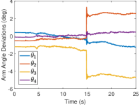
(a)

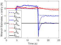
(b)

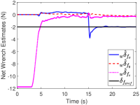
(c)

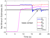
(d)

Figure 7: Results for the wrench estimation and interaction controller. (a-c) show the results for a static wrench application task where XPLORER is commanded to apply a 2N force on a wall (a) shows the deviation in the arm angles after being filtered, (b) shows the arm wrench, body wrench and total wrench in inertial x & y axis, (c) shows the net wrench as computed by (7) in the inertial frame (d) shows the net wrench results for a push-the-box experiment. The arrow marks the time when there is brief loss in contact due to unmodeled non-linear friction, however the contact is regained and the desired force objective is met.

VI-A2 Localization information

All the experiments are conducted in an indoor drone studio at ASU using a 10-camera motion capture system (OptiTrack, NaturalPoint Inc, OR) for obtaining the localization data and 3D pose estimation of XPLORER. The Root Mean Square Error (RMSE) for the localization data is $\pm 5$ cm. As mentioned in Section II-A, we use a ROS2-RTPS bridge to establish the communication between the high-level companion computer and the low-level flight controller. For every experiment presented, we run atleast three trials to validate the reliability and thoroughness of our proposed methods and obtain consistent performance for every trial. To make the article more organized, we chose to show results of only one trial from all the experiments.

VI-A3 Environment setup

To validate the performance of the algorithms, XPLORER was tested in two distinct environments containing obstacles. In the first scenario, a rectangular object measuring 1.22 m $\times$ 1.0 m was set up using acrylic panels, as illustrated in Fig. 5a. The use of transparent acrylic panels helped in tracking XPLORER’s movement through the obstacle via the motion capture system. This setup was designed to evaluate the exploration algorithm’s ability to navigate 90-degree turns and map the entire boundary of the obstacle to obtain its dimensions. The second scenario, depicted in Fig. 5(b), featured a corridor with slanted walls containing both concave and convex edges. This scenario effectively tests the algorithm’s ability to navigate through complex environments.

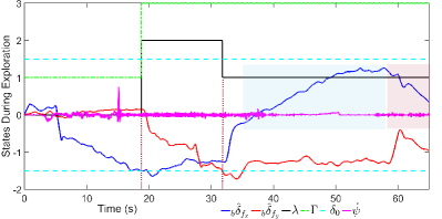
(a) Wall traversal

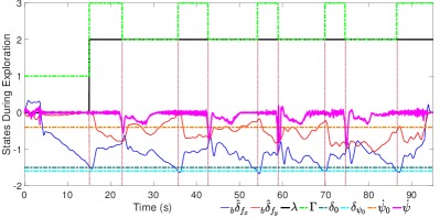
(b) Box traversal

Figure 8: Exploration results for two case scenarios. (a) shows the results for exploration of a wall-like structure. The exploration states are triggered when the threshold for $\delta_{0}$ are crossed. In this case only two states corresponding to $\Gamma=$1 and 3 are activated. The blue and red regions show that even during moving in state $\Gamma=$ 3, there is an external wrench observed in the $\pm$ $x$ direction indicating the presence of unmodeled frictional and wall-effects (b) shows the results for exploration of a box-like structure. The exploration states are switched when the thresholds for $\delta_{0}$ or $\dot{\psi}_{0}$ are crossed. In this case all three states corresponding to $\Gamma=$ 1, 2, 3 are activated. For both the plots, the vertical dotted lines show the time-instants where the thresholds are crossed to trigger the state-machine for deciding the exploration state. Units for the quantities are as follows: yawrate, $\dot{\psi}$, and yawrate threshold $\dot{\psi}_{0}$ are in rad/s, the wrenches ${}_{b}\hat{\delta}_{f_{x}}$ and ${}_{b}\hat{\delta}_{f_{y}}$ are in N, with non-dimensional values of $\lambda$ and $\Gamma$. Please note: the top view of the experiments (a) and (b) are shown in Fig.5.

VI-B External Wrench and Interaction Control

In this section, we present the results for the external wrench estimation algorithm and the designed interaction controller in Section III-E for two scenarios: the first for a static wall wrench application and the second for a box-pushing experiment. The results are shown in Fig. 7. The reference for this experiment is set to $\boldsymbol{\delta}_{f_{ref}}=[-2~{}0~{}0]^{T}$ for applying a 2 N force on the wall and $\boldsymbol{\delta}_{f_{ref}}=[-2~{}0~{}0]^{T}$ to push a box with 2 N by overcoming the friction on the carpet, both in the $x$ direction. Figure 7a shows the deviation of the arm angles which is used to calculate the arm wrench ${}_{w}\hat{\boldsymbol{\delta}}_{f_{a_{i}}}$ as shown in 7a. From Fig. 7b, it is seen that XPLORER is capable of exerting forces by using the admittance controller proposed. Similar results are obtained for pushing-the-box experiment as shown in Fig. 7d. As clearly seen, $\hat{\delta}_{f_{x}}$ converges to the given desired value while $\hat{\delta}_{f_{y}}$ and $\hat{\delta}_{f_{z}}$ converge to zero. For the second case when XPLORER tries to push a box, we see that there is loss in contact as shown by the arrow in Fig 7d, this is attributed to the slippage and the non-linear friction of real-life situations during the pushing experiment which was not accounted for while designing the interaction controller. We further demonstrate the safe-interaction policy in real-life in the Supplementary Video 1 for disturbance rejection, demonstrating compliant behaviour for safe human-aerial interaction and for the push-the-box scenario. Please note that, we refer to disturbance rejection as the flight mode when the interaction controller is not activated and compliant control for the case when the desired force is set to zero in the interaction controller. For the disturbance rejection, we observed that due to the deformable chassis, XPLORER returns to the setpoint without overshoot unlike its rigid counterparts where the disturbance leads to an increase in kinetic energies, thereby providing superior performance when compared to rigid conventional vehicles.

VI-C Contact-based Exploration

The exploratory algorithm proposed in Section IV-A is validated by real-time implementation on XPLORER.

VI-C1 Input data

The state machine in Fig. 3 requires clean input to function appropriately, so it is necessary to filter the external wrench estimate, $\hat{\boldsymbol{\delta}}_{f}$, and yaw rate, $\dot{\psi}$. To that end, a moving average filter with 50 samples is employed to filter ${}_{b}\hat{\boldsymbol{\delta}}_{f}$, while a low-pass filter is utilized to eliminate noise in the yaw rate, $\dot{\psi}$.

VI-C2 Parameters

The state machine for XPLORER relies on several parameters that require fine-tuning through trials. After extensive testing, we have determined the optimal values for these parameters that work well in all environments, and they are listed in Table II. To prevent excessive force on the objects in the environment and considering flight time, we limited ${\delta}_{0}$ to 1.5 N, though it is capable of exerting forces greater than 2 N. Furthermore, as XPLORER approaches right-angled corners/edges and rotates around those points, the corresponding yaw rate is measured to be 0.6 rad/s, which correlates to the force of 1.5 N being applied. Any increase of the applied force will result in a higher yaw rate. We choose 0.4 rad/s to detect such maneuver. For the Tactile-turning state, the controlled yaw maneuver is performed at 0.26 rad/s.

VI-C3 Results

XPLORER takes off and upon reaching a hover height of 0.7 m, it switches to Exploration state and moves in the positive x direction in the body frame. Once it detects the threshold external wrench, $\boldsymbol{\delta}_{0}$ in its movement direction, it switches to the Tactile-traversal state as described in Section IV-A. It maintains contact with the obstacle by applying $f_{des}$ force and moves across the environment. Throughout the flight, the yaw is in admittance ensuring two arms of the drone are in contact with the obstacle. Simultaneously, the map of the environment is also generated as shown in Fig. 5(b). In this experiment the Exploration and Tactile-traversal states are predominantly used for the navigation as shown in Fig. 8a and is shown in Supplementary Video 2.

VI-D Mapping

In the previous experiment, XPLORER successfully demonstrated its capability to navigate the boundary wall setup. Here, we demonstrate that it can perform loop closure, i.e., circumnavigate an obstacle and generate a complete map. This application enables extraction of the obstacle’s dimensions and its position in the environment, as detailed in Section IV-B.

VI-D1 Parameters

To perform mapping of the obstacle, an additional parameter $\boldsymbol{\delta_{map}}$ is introduced. It is set slightly higher than $f_{des}$ at 1.51 N to ensure that the mapping is initiated only when the vehicle has firm contact with the obstacle. Furthermore, an additional check is added to ensure that mapping is conducted only when XPLORER is flying. The other parameters used during this process can be found in Table II.

VI-D2 Results

Upon reaching a hover height of 0.7 m, XPLORER switches to Exploration state and moves in the positive x direction in the body frame. Upon encountering the wall, it proceeds to move across the obstacle until it reaches the corner where it releases and yaws. This triggers the Tactile-turning state which allows it to yaw in a controlled manner and establish contact with the adjacent wall, effectively switching back to the Tactile-traversal state. It continues traversing all the edges until it returns to the initial contact position, thereby achieving loop closure. From Fig. 8b we can infer that all three states corresponding to $\Gamma=[1-2-3]$ are activated whilst circumnavigating the obstacle. The generated map allows for the measurement of the dimension of the box, which is 1.231 m $\times$ 1.019 m and the actual dimensions are 1.22 m $\times$ 1.0 m. The accuracy is about 96.72% for computing the area of the box. One source of the mapping error is the imperfect position estimation (small errors from the motion capture system in our experiment), as it propagates in state estimation and to the point cloud data. The results are also shown in Supplementary Video 3.

VI-E Motion Planning

This section demonstrates the motion planning results for the two case scenarios described in Section V.

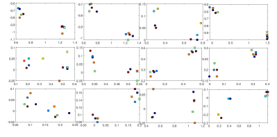
(a)

Figure 9: Experimental data for collision model. A set of 60 flight experiments was performed to generate a collision model for XPLORER for various collision scenarios. This plot denotes how pre-collision velocities map to the post-collision velocities in various scenarios. The x-axis denotes the $x$ direction velocity and y-axis denotes the $y$ direction velocity. The square markers show the pre-collision velocities and the circular markers represent the corresponding post-collision ones for each color, respectively.

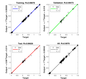
Figure 10: Validation results for the collision neural network showing the $R^{2}$ values obtained for the trained model. We see that the trained network is able to predict the post collision state with high accuracy.

VI-E1 Illustrative example

In this subsection we demonstrate that minimum time trajectories with collisions can be obtained with XPLORER. For this particular case scenario, we consider the collisions between the XPLORER and wall with the coefficient of restitution being 0.6, i.e., $e=-0.6$ in (17). Consider a wall at $a=0.5$, andan initial state $x_{0}=[-1~{}2]^{T}$ as the 0-jump minimum time can be calculated using (16) as 4 seconds.

Any generic point $(a,\zeta)$ after collision translates to $(a,-e\zeta)$, therefore the minimum time to reach $(a,\zeta)$ from an initial location $x_{0}=[-1~{}2]^{T}$ can be calculated using (18) as 1.756 seconds.

The corresponding bang-bang-jump-bang trajectory is shown in Fig. (11a). If there was no collision, XPLORER would have taken the trajectory shown in red to reach (0,0) in minimum time. However with a state-jump available, the optimal solution is to include the state-jump and undergo collision. Hence, XPLORER first reaches the wall with an optimal $\zeta^{*}$ velocity as calculated by argmin of (20) by using bang-bang control as shown by the blue lines. It then undergoes the state transition governed by $E$ to reach the point shown by the black star after which it again follows the black switching curve to reach to the origin (0,0).

VI-E2 Collision model

To verify the effectiveness of the bang-bang-jump-bang trajectories computed in the above subsection, it is crucial to identify the $E$ matrix in (17). Accordingly, from a set of 60 experiments, a data-driven collision model was developed to study the effects of collisions at various intensities and various angle of incidence for XPLORER. The experimental data collected are plotted as the pre-collision and post-collision velocities in Fig. 9. This collision model is crucial to identify the coefficient of restitution and the post-collision state of the vehicle for trajectory planning. Since the collisions for the deformable vehicle are highly nonlinear, a nonlinear regression model using neural networks was employed to develop the collision model. MATLAB Deep Learning Toolbox (MATLAB R2021b) was employed for the training using Levenberg-Marquardt method. Four features were identified to train the model: the $v_{x}^{-},v_{y}^{-}$ representing pre-collision state, angle of incidence to the collision plane, and type of collision. The angle of incidence is a function of the orientation of the vehicle, while the type of collision is either collide-to-stop (inelastic collision) or collide-to-decelerate (elastic collision). We choose 75$\%$ of the dataset for training and 25$\%$ for validation. The results for the collision network are given in Fig. 10 and we see that the accuracy is very high with a $R^{2}$ value of 0.99.

VI-E3 Experimental results

In this subsection, we experimentally demonstrate how collisions can be exploited to perform improved tracking and minimum time waypoint navigation with XPLORER by implementing the proposed method in Section V and utilizing the collision model developed in Section VI-E2. Towards this, we employ a reduced 1D collision model for which the coefficient of restitution was nearly 0.09 as identified from the network, thereby demonstrating almost perfect inelastic collisions. We accordingly substitute the value of $e$ in (14) as 0.09 for collide-to-stop scenarios and 0.4 for collide-to-decelerate scenarios. This capability is exploited to execute aggressive maneuvers where deceleration is achieved by colliding and expending energy to brake. We perform two sets of experiments when XPLORER is commanded to reach a particular setpoint where the wall is placed and these results are compared to the performance of a conventional waypoint tracking with perfectly tuned gains.

The rise time ($\tau_{r}$) and the settling time ($\tau_{s}$) are chosen as the metrics to evaluate the performance of CATAAN for XPLORER for all cases. The results for the conventional, collision-exclusive trajectory is shown in Fig. 11b. In this case, the vehicle first reaches the setpoint, overshoots and then tries to minimize the error by slowly converging to the reference. The $\tau_{r}$ and $\tau_{s}$ are noted to be 2.27 and 8.995 seconds, respectively. Furthermore, over three trials the RMSE error was around $\pm$ 3cm for this case. For collision-inclusive trajectories, the experimental results show that XPLORER reaches the wall with maximum velocity and the $e$ is low enough in order to stop the vehicle at the wall itself by absorbing the collision energies. This demonstrates the collide-to-stop maneuver. Consequently, the vehicle stops near the wall almost instantaneously as shown by the plots in Fig. 11c. The $\tau_{r}$ and $\tau_{s}$ are calculated to be 1.046 and 5.292 seconds, respectively which are faster than the conventional trajectories. For the case where the vehicle performs collide-to-decelerate and regulates itself to a setpoint beyond the wall, and results in Fig. 11d show significantly shorter convergence time with $\tau_{r}=1.685$ seconds and $\tau_{s}=3.631$ seconds, respectively. The low settling time for the later case as compared to a sudden stop at the wall can be attributed to the wall effect which affects the performance of the vehicle for the collide-to-stop case as also noted in Section VI-B. We also noted that the RMSE values over 6 trials for the collision-inclusive trajectories were $\pm$ 0.5cm showing improved tracking accuracy than the conventional maneuvers. This can be attributed to the dissipation of kinetic energies upon collision, leading to improved decelerating performance. All the experimental results for CATAAN are shown in Supplementary Video 4 as well.

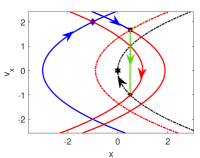
(a) Simulation Results

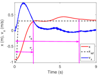
(b) Without collision

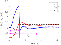
(c) Collide-to-stop

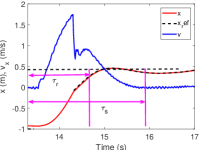
(d) Collide-to-decelerate

Figure 11: Results for CATAAN applied on XPLORER. (a) Simulation results and the phase-portrait for the proposed collision-inclusive arcs with state-jumps. The blue-blue-green-black states depict the minimum-time trajectories as compared to the conventional red-black curve as obtained from bang-bang control law without collisions. (b) Experimental results for a case without collision, with $\tau_{r}=2.27$ and $\tau_{s}=8.995$ seconds. (c) Experimental results for the collide-to-stop maneuver, $\tau_{r}=1.046$ and $\tau_{s}=5.292$ seconds (d) Experimental results for the case collide-to-decelerate, $\tau_{r}=1.685$ and $\tau_{s}=3.631$ seconds.

VII Conclusion

In this work we presented a complete autonomous planning and control framework for a passive deformable quadrotor, XPLORER, to perform physical interaction tasks, including exploring unknown environments through contact, generating maps and planning minimum-time and collision-inclusive trajectories. As the first step, the acceleration-based wrench estimation algorithm was modified to account for the change in morphology to get accurate wrench estimates. The wrench estimation algorithm was verified by experiments for a static wrench application and a pushing experiment. Furthermore, a novel exploration and mapping scheme was presented which adaptively switched between the various available flight modes to explore an unknown flight space. This algorithm was successfully implemented and validated to generate a map of the space for a wall-like object and a box-like object. Finally a novel collision-inclusive trajectory planner, CATAAN, was introduced which generated minimum-time paths by considering the state jumps introduced by collisions. With the information of the map generated in the previous step, this planner can successfully generate minimum-time paths, even faster than those obtained from classical bang-bang control laws without leveraging collisions. The results showed that CATAAN successfully generated minimum time paths which was 40.38$\%$ faster than the conventional trajectory tracking methods. Furthermore, due to the dissipation of the kinetic energies after collision, the deceleration was faster and the tracking performance was significantly improved.

Given the comprehensive end-to-end framework for exploration and navigation, there is still room for improvement from the low-level and wrench estimation perspective. Future work will look into collision isolation for the exact wrench estimate on the arm and model individually the various external wrenches instead of the lumped model assumption. This is particularly beneficial since, in our current algorithm, we do not model wall-effects which cause XPLORER to get stuck near corners and increase in friction during the Tactile-traversal modes. In such scenarios, a viscous drag model for friction also fails and significant aerodynamic studies have to be conducted to study this phenomena.

Furthermore, the assumption that the external wrench is applied at the arm at the motor location, can sometimes lead to inaccurate results, leaving a lot of room for improvement. The current mapping framework relies entirely on localization data obtained from the motion-capture system, exploring the implementation of onboard sensors and state estimation techniques will enable the vehicle to be deployed in actual environments. The sensor fusion approach can be considered for the mapping framework, making it possible to fuse the generated tactile-based map with those produced by LiDAR or vision systems. For the collision-inclusive trajectory planner, we demonstrated 1D collision benefits, future-work can look into extending this idea to 3D for achieving minimum-time trajectories for any kind of vehicle not only limited to the passive deformable quadrotors. All of the future work will make future robots ready to embrace and potentially benefit from collisions in real-world applications such as infrastructure inspection, search and rescue, and environmental monitoring.

VIII Acknowledgement

The authors would like to thank YiZhuang Garrard for the engaging brainstorming sessions and Bill Nguyen for his help designing filters for the implementation of the wrench estimation algorithms.

References

- [1] M. R. Freeman, M. M. Kashani, and P. J. Vardanega, “Aerial robotic technologies for civil engineering: established and emerging practice,” Journal of Unmanned Vehicle Systems, vol. 9, no. 2, pp. 75–91, 2021.
- [2] F. Ruggiero, V. Lippiello, and A. Ollero, “Aerial manipulation: A literature review,” IEEE Robotics and Automation Letters, vol. 3, no. 3, pp. 1957–1964, 2018.
- [3] D. Hausamann, W. Zirnig, G. Schreier, and P. Strobl, “Monitoring of gas pipelines–a civil uav application,” Aircraft Engineering and Aerospace Technology, vol. 77, no. 5, pp. 352–360, 2005.
- [4] S. Mishra, D. F. Syed, M. Ploughe, and W. Zhang, “Autonomous vision-guided object collection from water surfaces with a customized multirotor,” IEEE/ASME Transactions on Mechatronics, vol. 26, no. 4, pp. 1914–1922, 2021.
- [5] S. Kim, S. Choi, and H. J. Kim, “Aerial manipulation using a quadrotor with a two dof robotic arm,” in 2013 IEEE/RSJ International Conference on Intelligent Robots and Systems, pp. 4990–4995, IEEE, 2013.
- [6] A. Suarez, G. Heredia, and A. Ollero, “Lightweight compliant arm for aerial manipulation,” in 2015 IEEE/RSJ International Conference on Intelligent Robots and Systems, pp. 1627–1632, IEEE, 2015.
- [7] J. L. Schonberger and J.-M. Frahm, “Structure-from-motion revisited,” in Proceedings of the IEEE Conference on Computer Vision and pattern recognition, pp. 4104–4113, 2016.
- [8] D. Falanga, K. Kleber, S. Mintchev, D. Floreano, and D. Scaramuzza, “The foldable drone: A morphing quadrotor that can squeeze and fly,” IEEE Robotics and Automation Letters, vol. 4, no. 2, pp. 209–216, 2019.
- [9] N. Meiri and D. Zarrouk, “Flying star, a hybrid crawling and flying sprawl tuned robot,” in 2019 International Conference on Robotics and Automation, pp. 5302–5308, IEEE, 2019.
- [10] N. Bucki, J. Tang, and M. W. Mueller, “Design and control of a midair-reconfigurable quadcopter using unactuated hinges,” IEEE Transactions on Robotics, 2022.
- [11] K. Patnaik and W. Zhang, “Towards reconfigurable and flexible multirotors: A literature survey and discussion on potential challenges,” International Journal of Intelligent Robotics and Applications, vol. 5, no. 3, pp. 365–380, 2021.
- [12] K. Patnaik, S. Mishra, S. M. R. Sorkhabadi, and W. Zhang, “Design and control of squeeze: A spring-augmented quadrotor for interactions with the environment to squeeze-and-fly,” in 2020 IEEE/RSJ International Conference on Intelligent Robots and Systems, pp. 1364–1370, IEEE, 2020.
- [13] Z. Liu and K. Karydis, “Toward impact-resilient quadrotor design, collision characterization and recovery control to sustain flight after collisions,” in 2021 IEEE International Conference on Robotics and Automation, pp. 183–189, IEEE, 2021.
- [14] K. Patnaik, S. Mishra, Z. Chase, and W. Zhang, “Collision recovery control of a foldable quadrotor,” in 2021 IEEE/ASME International Conference on Advanced Intelligent Mechatronics, pp. 418–423, 2021.
- [15] P. H. Nguyen, K. Patnaik, S. Mishra, P. Polygerinos, and W. Zhang, “A soft-bodied aerial robot for collision resilience and contact-reactive perching,” Soft Robotics, 2023.
- [16] S. Haddadin, Towards safe robots: approaching Asimov’s 1st law, vol. 90. Springer, 2013.
- [17] A. De Luca and R. Mattone, “Sensorless robot collision detection and hybrid force/motion control,” in Proceedings of the 2005 IEEE international conference on robotics and automation, pp. 999–1004, IEEE, 2005.
- [18] B. Yüksel, C. Secchi, H. H. Bülthoff, and A. Franchi, “A nonlinear force observer for quadrotors and application to physical interactive tasks,” in 2014 IEEE/ASME international conference on advanced intelligent mechatronics, pp. 433–440, IEEE, 2014.
- [19] M. Orsag, C. Korpela, P. Oh, S. Bogdan, and A. Ollero, Aerial manipulation. Springer, 2018.
- [20] V. Serbezov, H. Panayotov, M. Todorov, and S. Penchev, “Application of multi-axis force/torque sensor system for experimental study of small unmanned aerial vehicles propulsion systems–preliminary results,” vol. 878, no. 1, p. 012039, 2020.
- [21] A. Ollero, G. Heredia, A. Franchi, G. Antonelli, K. Kondak, A. Sanfeliu, A. Viguria, J. R. Martinez-de Dios, F. Pierri, J. Cortés, et al., “The aeroarms project: Aerial robots with advanced manipulation capabilities for inspection and maintenance,” IEEE Robotics & Automation Magazine, vol. 25, no. 4, pp. 12–23, 2018.
- [22] F. Ruggiero, J. Cacace, H. Sadeghian, and V. Lippiello, “Impedance control of vtol uavs with a momentum-based external generalized forces estimator,” in 2014 IEEE international conference on robotics and automation, pp. 2093–2099, IEEE, 2014.
- [23] F. Ruggiero, J. Cacace, H. Sadeghian, and V. Lippiello, “Passivity-based control of vtol uavs with a momentum-based estimator of external wrench and unmodeled dynamics,” Robotics and Autonomous Systems, vol. 72, pp. 139–151, 2015.
- [24] M. Ryll, G. Muscio, F. Pierri, E. Cataldi, G. Antonelli, F. Caccavale, D. Bicego, and A. Franchi, “6d interaction control with aerial robots: The flying end-effector paradigm,” The International Journal of Robotics Research, vol. 38, no. 9, pp. 1045–1062, 2019.
- [25] C. D. McKinnon and A. P. Schoellig, “Unscented external force and torque estimation for quadrotors,” in 2016 IEEE/RSJ International Conference on Intelligent Robots and Systems, pp. 5651–5657, IEEE, 2016.
- [26] T. Tomić, C. Ott, and S. Haddadin, “External wrench estimation, collision detection, and reflex reaction for flying robots,” IEEE Transactions on Robotics, vol. 33, no. 6, pp. 1467–1482, 2017.
- [27] P. Pfändler, K. Bodie, U. Angst, and R. Siegwart, “Flying corrosion inspection robot for corrosion monitoring of civil structures–first results,” in SMAR 2019-Fifth Conference on Smart Monitoring, Assessment and Rehabilitation of Civil Structures-Program, pp. We–4, SMAR, 2019.
- [28] J. Hu, S. Zhang, E. Chen, and W. Li, “A review on corrosion detection and protection of existing reinforced concrete (rc) structures,” Construction and Building Materials, vol. 325, p. 126718, 2022.
- [29] K. Alexis, G. Darivianakis, M. Burri, and R. Siegwart, “Aerial robotic contact-based inspection: planning and control,” Autonomous Robots, vol. 40, pp. 631–655, 2016.
- [30] K. Bodie, M. Brunner, M. Pantic, S. Walser, P. Pfändler, U. Angst, R. Siegwart, and J. Nieto, “Active interaction force control for contact-based inspection with a fully actuated aerial vehicle,” IEEE Transactions on Robotics, vol. 37, no. 3, pp. 709–722, 2020.
- [31] M. Tognon, H. A. T. Chávez, E. Gasparin, Q. Sablé, D. Bicego, A. Mallet, M. Lany, G. Santi, B. Revaz, J. Cortés, et al., “A truly-redundant aerial manipulator system with application to push-and-slide inspection in industrial plants,” IEEE Robotics and Automation Letters, vol. 4, no. 2, pp. 1846–1851, 2019.
- [32] G. Nava, Q. Sablé, M. Tognon, D. Pucci, and A. Franchi, “Direct force feedback control and online multi-task optimization for aerial manipulators,” IEEE Robotics and Automation Letters, vol. 5, no. 2, pp. 331–338, 2019.
- [33] W. Zhang, L. Ott, M. Tognon, and R. Siegwart, “Learning variable impedance control for aerial sliding on uneven heterogeneous surfaces by proprioceptive and tactile sensing,” IEEE Robotics and Automation Letters, vol. 7, no. 4, pp. 11275–11282, 2022.
- [34] B. Brogliato and B. Brogliato, Nonsmooth mechanics, vol. 3. Springer, 1999.
- [35] J.-C. Zufferey, A. Beyeler, and D. Floreano, “Optic flow to steer and avoid collisions in 3d,” Flying Insects and Robots, pp. 73–86, 2010.
- [36] D. Schafroth, S. Bouabdallah, C. Bermes, and R. Siegwart, “From the test benches to the first prototype of the mufly micro helicopter,” Journal of Intelligent and Robotic Systems, vol. 54, pp. 245–260, 2009.
- [37] R. He, A. Bachrach, and N. Roy, “Efficient planning under uncertainty for a target-tracking micro-aerial vehicle,” in 2010 IEEE International Conference on Robotics and Automation, pp. 1–8, IEEE, 2010.
- [38] S. Shen, N. Michael, and V. Kumar, “Autonomous multi-floor indoor navigation with a computationally constrained mav,” in 2011 IEEE International Conference on Robotics and Automation, pp. 20–25, IEEE, 2011.
- [39] D. Scaramuzza, M. C. Achtelik, L. Doitsidis, F. Friedrich, E. Kosmatopoulos, A. Martinelli, M. W. Achtelik, M. Chli, S. Chatzichristofis, L. Kneip, et al., “Vision-controlled micro flying robots: from system design to autonomous navigation and mapping in gps-denied environments,” IEEE Robotics & Automation Magazine, vol. 21, no. 3, pp. 26–40, 2014.
- [40] A. Briod, P. Kornatowski, A. Klaptocz, A. Garnier, M. Pagnamenta, J.-C. Zufferey, and D. Floreano, “Contact-based navigation for an autonomous flying robot,” in 2013 IEEE/RSJ International Conference on Intelligent Robots and Systems, pp. 3987–3992, IEEE, 2013.
- [41] P. De Petris, H. Nguyen, M. Kulkarni, F. Mascarich, and K. Alexis, “Resilient collision-tolerant navigation in confined environments,” in 2021 IEEE International Conference on Robotics and Automation, pp. 2286–2292, IEEE, 2021.
- [42] T. Lew, T. Emmei, D. D. Fan, T. Bartlett, A. Santamaria-Navarro, R. Thakker, and A.-a. Agha-mohammadi, “Contact inertial odometry: collisions are your friends,” in Robotics Research: The 19th International Symposium ISRR, pp. 938–958, Springer, 2022.
- [43] M. Zhao, K. Okada, and M. Inaba, “Enhanced modeling and control for multilinked aerial robot with two dof force vectoring apparatus,” IEEE Robotics and Automation Letters, vol. 6, no. 1, pp. 135–142, 2020.
- [44] N. Khedekar, F. Mascarich, C. Papachristos, T. Dang, and K. Alexis, “Contact–based navigation path planning for aerial robots,” in 2019 International Conference on Robotics and Automation, pp. 4161–4167, IEEE, 2019.
- [45] L. M. Gonzalez de Santos, E. Frias Nores, J. Martinez Sanchez, and H. Gonzalez Jorge, “Indoor path-planning algorithm for uav-based contact inspection,” Sensors, vol. 21, no. 2, p. 642, 2021.
- [46] J. Zha and M. W. Mueller, “Exploiting collisions for sampling-based multicopter motion planning,” in 2021 IEEE International Conference on Robotics and Automation, pp. 7943–7949, IEEE, 2021.
- [47] W. Zhen, Y. Hu, H. Yu, and S. Scherer, “Lidar-enhanced structure-from-motion,” in 2020 IEEE International Conference on Robotics and Automation, pp. 6773–6779, IEEE, 2020.
- [48] A. J. Davison, “Real-time simultaneous localisation and mapping with a single camera,” in Computer Vision, IEEE International Conference on, vol. 3, pp. 1403–1403, IEEE Computer Society, 2003.
- [49] R. Mur-Artal, J. M. M. Montiel, and J. D. Tardos, “Orb-slam: a versatile and accurate monocular slam system,” IEEE Transactions on Robotics, vol. 31, no. 5, pp. 1147–1163, 2015.
- [50] J. Zhang and S. Singh, “Loam: Lidar odometry and mapping in real-time.,” Robotics: Science and Systems, vol. 2, no. 9, pp. 1–9, 2014.
- [51] D. Cattaneo, M. Vaghi, A. L. Ballardini, S. Fontana, D. G. Sorrenti, and W. Burgard, “Cmrnet: Camera to lidar-map registration,” in 2019 IEEE intelligent transportation systems conference, pp. 1283–1289, IEEE, 2019.
- [52] P. De Petris, S. J. Carlson, C. Papachristos, and K. Alexis, “Collision-tolerant aerial robots: A survey,” arXiv preprint arXiv:2212.03196, 2022.
- [53] S. Mintchev, S. de Rivaz, and D. Floreano, “Insect-inspired mechanical resilience for multicopters,” IEEE Robotics and Automation Letters, vol. 2, no. 3, pp. 1248–1255, 2017.
- [54] P. H. Nguyen, K. Patnaik, S. Mishra, P. Polygerinos, and W. Zhang, “A soft-bodied aerial robot for collision resilience and contact-reactive perching,” Soft Robotics, 2023.
- [55] A. Fabris, E. Aucone, and S. Mintchev, “Crash 2 squash: An autonomous drone for the traversal of narrow passageways,” Advanced Intelligent Systems, vol. 4, no. 11, p. 2200113, 2022.
- [56] A. Cristofaro, C. Possieri, and M. Sassano, “Time-optimal control for the hybrid double integrator with state-driven jumps,” in 2019 IEEE 58th Conference on Decision and Control, pp. 6301–6306, IEEE, 2019.
- [57] K. Patnaik and W. Zhang, “Adaptive attitude control for foldable quadrotors,” IEEE Control Systems Letters, 2023.
- [58] Q.-Y. Zhou, J. Park, and V. Koltun, “Open3D: A modern library for 3D data processing,” arXiv:1801.09847, 2018.