Building One-class Detector for Anything: Open-vocabulary Zero-shot OOD Detection Using Text-image Models

Abstract

We focus on the challenge of out-of-distribution (OOD) detection in deep learning models, a crucial aspect in ensuring reliability. Despite considerable effort, the problem remains significantly challenging in deep learning models due to their propensity to output over-confident predictions for OOD inputs. We propose a novel one-class open-set OOD detector that leverages text-image pre-trained models in a zero-shot fashion and incorporates various descriptions of in-domain and OOD. Our approach is designed to detect anything not in-domain and offers the flexibility to detect a wide variety of OOD, defined via fine- or coarse-grained labels, or even in natural language. We evaluate our approach on challenging benchmarks including large-scale datasets containing fine-grained, semantically similar classes, distributionally shifted images, and multi-object images containing a mixture of in-domain and OOD objects. Our method shows superior performance over previous methods on all benchmarks.
Code is available at https://github.com/gyhandy/One-Class-Anything

1 Introduction

Out-of-distribution detection (OOD) is essential for ensuring the reliability of machine learning systems. When a machine learning system is deployed in the real world, it may encounter unexpected abnormal inputs that are not from the same distribution as the training data. Detection and removal of OOD inputs prevents the machine learning (ML) system from making incorrect predictions that could otherwise lead to serious failures especially in safety-critical applications. For example, a person classification model is trained to localize people in images. If an image that does not contain a person, but instead contains an animal or a sculpture, the model may erroneously label the non-person as a person. Accurate and reliable one-class detection is of paramount importance in life-critical applications; for example, correctly perceiving persons in autonomous driving systems.

Although OOD detection has been studied previously in traditional ML models [34, 5], deep learning models are known to output over-confident predictions for OOD inputs, making OOD detection in deep learning much more challenging. Recent efforts have focused on developing methods to correct for the naive softmax probability [8, 18, 10, 20], using deep neural representations to measure the distance to the training distribution [16, 30, 37, 7], leveraging OOD data to learn a more precise decision boundary between in-domain and OOD [9, 31], and using deep density models to measure the likelihood under the training distribution [4, 29, 24, 23].

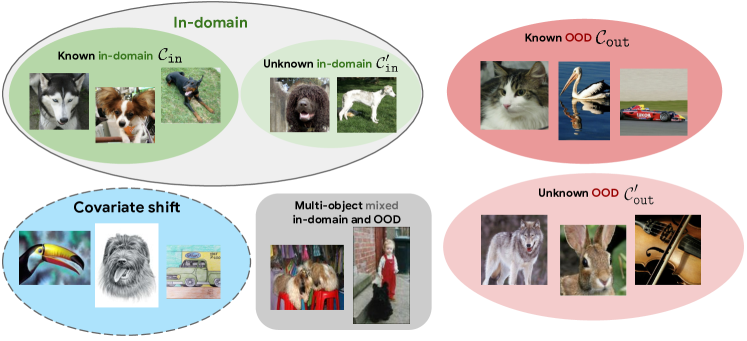
Figure 1: We study the one-class OOD detection problem where OOD can be anything not in-domain. Example of building a dog detector with some known dogs $\mathcal{C}_{\texttt{in}}=${Husky, Papillon, Dobermann} and known non-dogs $\mathcal{C}_{\texttt{out}}=${Cat, Bird, Person}. When deploying such a one-class detector in the real world, it’s important for it to be robust to several different types of shifts: (1) Unknown in-domain classes include new species of dogs, and unknown OOD such as wolves, bunnies, violins, (2) Multi-object cases (cats along with dogs, persons along with dogs), (3) Covariate shift (drawings of dogs, painting of a bird, cartoon car, etc).

For evaluation, most OOD detection methods use one dataset as in-domain and another dataset as OOD. For example, the CIFAR100 vs CIFAR10 [29, 30, 7, 16], or ImageNet vs Places365 [10, 22] benchmark datasets; both have in-domain data that consists of a set of classes, and OOD data comprised of a different set of classes that are non-overlapping with the in-domain. That scenario treats OOD classes as a closed set. However, in realistic scenarios, in-domain data often consists of a set of classes belonging to a unified high-level superclass, and OOD data is anything that is not in that superclass, which can be viewed as an open-set one-class anomaly detection problem [14, 25]. For example, the OOD detection in the person identification scanario is to detect anything that is non-person.

The most straightforward approach for building a one-class OOD detector is to train a binary classifier for in-domain and OOD classes [1]. However, since the OOD space is large (anything that is not in-domain) and often includes classes that follow a long-tail distribution [31], it is impossible to include all the possible OOD data when training. Consequently, a model trained on a subset of OOD data may suffer from poor generalization to the unseen OOD at test time. Another approach is to learn the distribution of the in-domain data without using prior knowledge of OOD [32, 3, 44, 13, 26, 23, 2], but that approach cannot leverage the knowledge of known OOD data which can help with learning a more precise boundary. Another issue with the existing one-class OOD work is that the datasets used for evaluation are fairly simple and small scale as MNIST and SVHN. Usually one class serves as in-domain and the remaining classes are OOD (such as using 1 as in-domain and the numbers 2 through 9 as OOD). That testing regime does not fully explore a setting with the open-set assumption that OOD can be anything not in-domain, including, for example, images of non-numbers.

Recently, large pretrained text-image models such as CLIP (Contrastive Language-Image Pretraining) [27], and LiT [43] learn the image and text representations simultaneously from massive image captioning data, and can be used as a zero-shot classifier at inference time by comparing the similarity between the class label and the image in the embedding space. It has also shown that the maximum softmax score from the zero-shot classifier is a reasonably good confidence score for OOD detection [22]. However, that method only takes the in-domain class labels without leveraging the OOD information. Fort et al. [7], Esmaeilpour et al. [6] propose a weaker form of outlier exposure (OE) by including OOD class names into the label set without any accompanying images, and use the sum of the softmax over the OOD class labels as the OOD score. Since the methods were only evaluated on closed-set tasks, it is unclear how well the methods would perform on one-class OOD detection problem which evaluate the generalization ability with unseen classes. We are also interested in evaluating on large-scaled datasets such as ImageNet, and its variants to see how well the methods perform on fine-grained and semantically similar classes, and on distributional shifted data.

In this work, we develop a one-class open-set OOD detector using text-image pretrained models in a zero-shot fashion. Our one-class open-set OOD detector detects anything that is not in-domain, contrary to methods that specify a restricted set of predefined OOD classes. Our method can be used to detect any type of OOD, defined either in fine-grained or coarse-grained labels, or even in natural language, through customizing the text labels in the text-image zero-shot classifier. We evaluate our method on large-scaled challenging benchmarks to mimic real-world scenarios, and test with (1) images from unseen classes, (2) distribution shifted images, (3) multi-object images that are may contain a mixture of in-domain and OOD objects. See Figure 1 for an overview. We show our method consistently outperforms the previous methods on all the challenging benchmarks.

Our contributions are the following:

• We find that previous methods [7, 22] do not work well on OOD detection for samples outside of the predefined class sets. We propose better OOD scores that utilize the in-domain and OOD labels and show that they consistently perform best for detecting hard samples from long-tail unseen classes and under distribution shifts.

• Our proposed method is flexible enough to incorporate various definition of in-domain and OOD. Because our method is based on text-image models, users can easily customize the definitions of in-domain and OOD via text labels, for example using class names at different hierarchical levels, or even including natural language sentences.

• We tackle the challenging OOD detection for multi-object images that contain a mixture of in-domain and OOD objects. Integrating our scores into powerful segmentation models [15, 19], we are able to identify images with mixed in-domain and OOD objects, outperforming the baselines.

2 Methods

2.1 Background

Contrastively pre-trained text-image models can be used as zero-shot classification models [27]. Text-image models consist of an image encoder $f_{\texttt{img}}(\cdot)$ and a text encoder $f_{\texttt{txt}}(\cdot)$. Given an input image ${\bm{x}}$ and an input text $t$, the encoders produce embeddings ${\bm{z}}_{\texttt{img}}=f_{\texttt{img}}({\bm{x}})$ and ${\bm{z}}_{\texttt{txt}}=f_{\texttt{txt}}(t)$ for the image and the text respectively. The model is trained to maximize the cosine similarity between the ${\bm{z}}_{\texttt{img}}$ and ${\bm{z}}_{\texttt{txt}}$ from the paired $\{\texttt{image},\texttt{caption}\}$ data, and minimize the cosine similarity between the unpaired data. At test time, to predict the class of an image ${\bm{x}}$, we first encode the candidate class names $\mathcal{C}=\{c_{1},\dots,c_{n}\}$ using the text encoder individually, $\{{\bm{z}}_{\texttt{txt}}^{1},\dots,{\bm{z}}_{\texttt{txt}}^{n}\}$. Then we compute the cosine similarity between the image ${\bm{x}}$ and a set of candidate class names $\mathcal{C}$,

$$\mathtt{logits}({\bm{x}},\mathcal{C})=\left[{\bm{z}}_{\texttt{img}}\cdot{\bm{z}}_{\texttt{txt}}^{1},\cdots,{\bm{z}}_{\texttt{img}}\cdot{\bm{z}}_{\texttt{txt}}^{n}\right],$$

The predicted class for this image ${\bm{x}}$ is $\hat{c}({\bm{x}})=\mathrm{argmax}_{c}\ \mathtt{logits}({\bm{x}},\mathcal{C})$.

For the problem of OOD detection, given a set of in-domain class labels $\mathcal{C}_{\texttt{in}}=\{c^{\texttt{in}}_{1},\dots,c^{\texttt{in}}_{N}\}$, Ming et al. [22] propose to use the $\max_{c}p(c|{\bm{x}},\mathcal{C}_{\texttt{in}})$ as the confidence score, where $p(c|{\bm{x}},\mathcal{C}_{\texttt{in}})$ is the element of $\mathrm{softmax}\left(\mathtt{logits}({\bm{x}},\mathcal{C}_{\texttt{in}})\right)$ corresponding to the label $c$, i.e. $p(c|{\bm{x}},\mathcal{C}_{\texttt{in}})=\frac{e^{w_{c}}}{\sum_{j\in\mathcal{C}_{\texttt{in}}}e^{w_{j}}},w_{c}={\bm{z}}_{\texttt{img}}\cdot{\bm{z}}_{\texttt{txt}}^{c}$ . The $\mathtt{logits}$ can be further scaled by a temperature factor. A high confidence score indicates that the input image is likely to be from one of the $\mathcal{C}_{\texttt{in}}$ classes, and thus in-domain. The corresponding OOD score is defined as

$$S_{\texttt{-max\_prob}}({\bm{x}})=-\max_{c\in\mathcal{C_{\texttt{in}}}}p(c|{\bm{x}},\mathcal{C}_{\texttt{in}})$$ (1)

The above method assumes that only a set of in-domain class labels is available, i.e., without exposure to OOD labels. However, although it can be difficult to obtain OOD images, it is often very easy to produce a set of possible OOD labels. In that setting, [7, 6] proposes to include the OOD labels $\mathcal{C}_{\texttt{out}}=\{c_{1}^{\texttt{out}},\dots,c_{M}^{\texttt{out}}\}$ into the candidate label set $\mathcal{C}=\mathcal{C}_{\texttt{in}}\cup\mathcal{C}_{\texttt{out}}$, to utilize the knowledge as a weak form of outlier exposure, without using any OOD images for training. Then the $\mathtt{logits}$ are:

$$\mathtt{logits}({\bm{x}},\mathcal{C}_{\texttt{in}}\cup\mathcal{C}_{\texttt{out}})=\left[{\bm{z}}_{\texttt{img}}\cdot{\bm{z}}_{\texttt{txt}}^{1},\cdots,{\bm{z}}_{\texttt{img}}\cdot{\bm{z}}_{\texttt{txt}}^{N},{\bm{z}}_{\texttt{img}}\cdot{\bm{z}}_{\texttt{txt}}^{N+1},\cdots,{\bm{z}}_{\texttt{img}}\cdot{\bm{z}}_{\texttt{txt}}^{N+M}\right]$$

And the OOD score is defined as

$$S_{\texttt{sum\_out\_prob}}({\bm{x}})=\sum_{c\in\mathcal{C_{\texttt{out}}}}p(c|{\bm{x}},\mathcal{C}_{\texttt{in}}\cup\mathcal{C}_{\texttt{out}}),$$ (2)

where $p(c|{\bm{x}},\mathcal{C}_{\texttt{in}}\cup\mathcal{C}_{\texttt{out}})=\frac{e^{w_{c}}}{\sum_{j\in\mathcal{C_{\texttt{in}}}}e^{w_{j}}+\sum_{k\in\mathcal{C_{\texttt{out}}}}e^{w_{k}}}$, $w_{c}={\bm{z}}_{\texttt{img}}\cdot{\bm{z}}_{\texttt{txt}}^{c}$.

Figure 2: Our methods utilize in-domain and OOD label sets. When in-domain classes $\mathcal{C}_{\texttt{in}}$ are comprised only of dog breeds, a butterfly may be mistaken for a Papillon dog, possibly due to the similar shape and color to the dog’s ears. However, when a OOD set $\mathcal{C}_{\texttt{out}}$ is included consisting of the class name “butterfly”, or a more precise butterfly type “red admiral butterfly”, or a text description “a photograph of red admiral butterfly”, the image embedding’s similarity with this label pushes down the probabilities with the in-domain dog breeds, correctly identifying the image as OOD. Thus our method $S_{\texttt{-max\_in\_prob}}$ has better separation between in-domain and OOD compared to the baseline $S_{\texttt{-max\_prob}}$, as shown on the left 2D histograms.

2.2 Our methods: OOD scores utilizing in-domain and OOD label sets

In this work, we follow on the same setting as Fort et al. [7] because in the real scenario it is generally easy to produce a set of OOD class labels. For example, for the problem of detecting non-persons in a person detection system, it is easy to create a list of non-person labels that are commonly shown in photos, $\mathcal{C}_{\texttt{out}}=${animals, buildings, cars, food, $\dots$}. We would like to exploit these labels to improve the decision boundary between in- and out-of distribution. Note that $\mathcal{C}_{\texttt{out}}$ may not cover all the sub-types in OOD space due to the long-tail distribution. That is why we assume there are unseen classes $\mathcal{C}_{\texttt{out}}^{\prime}$. Note that our methods are only based on $\mathcal{C}_{\texttt{out}}$ not $\mathcal{C}_{\texttt{out}}^{\prime}$. We will show the good generalization of our methods on unseen classes in Section 3.1.

Suppose we have an in-domain label set $\mathcal{C}_{\texttt{in}}$ and a OOD label set $\mathcal{C}_{\texttt{out}}$. Inspired by [22], we first propose the maximum softmax probability over the $\mathcal{C}_{\texttt{in}}$ as the confidence score, and its negative as the OOD score,

$$S_{\texttt{-max\_in\_prob}}({\bm{x}})=-\max_{c\in\mathcal{C_{\texttt{in}}}}p(c|{\bm{x}},\mathcal{C}_{\texttt{in}}\cup\mathcal{C}_{\texttt{out}}).$$ (3)

Note that our score is different from Ming et al. [22] in the sense that we apply the softmax normalization over all labels $\mathcal{C}=\mathcal{C}_{\texttt{in}}\cup\mathcal{C}_{\texttt{out}}$, while Ming et al. [22] only applies softmax on $\mathcal{C}_{\texttt{in}}$. Including $\mathcal{C}_{\texttt{out}}$ in the label sets is important for OOD detection, as shown in Figure 2. An OOD image may have relatively high similarity to one of the $\mathcal{C}_{\texttt{in}}$ classes due to spurious features. Once $\mathcal{C}_{\texttt{out}}$ is included, the OOD image’s similarity with the OOD labels pushes down the probabilities with the in-domain $\mathcal{C}_{\texttt{in}}$ classes, correctly identifying the image as OOD.

Alternatively, we have the maximum softmax probability over the $\mathcal{C}_{\texttt{out}}$ as another candidate OOD score,

$$S_{\texttt{max\_out\_prob}}({\bm{x}})=\max_{c\in\mathcal{C_{\texttt{out}}}}p(c|{\bm{x}},\mathcal{C}_{\texttt{in}}\cup\mathcal{C}_{\texttt{out}}).$$ (4)

We also consider a score based on $\mathtt{logits}$ without softmax normalization, as Hendrycks et al. [10] previously show that in the larger-scale and real-world settings, the un-normalized maximum logit outperforms the normalized maximum softmax probability for OOD detection in the single modal models. We propose the OOD score as,

$$S_{\texttt{max\_logit\_diff}}({\bm{x}})= \max_{d\in\mathcal{C_{\texttt{out}}}}w_{d}-\max_{c\in\mathcal{C_{\texttt{in}}}}w_{c}.$$ (5)

The score measures if a test image has a higher similarity to any of the classes in $\mathcal{C}_{\texttt{out}}$ in comparison to the similarity to any of the classes in $\mathcal{C}_{\texttt{in}}$. Having a reference for the similarity to $\mathcal{C}_{\texttt{in}}$ is helpful for understanding if the similarity to $\mathcal{C}_{\texttt{out}}$ is truly high or not. $S_{\texttt{max\_logit\_diff}}({\bm{x}})>0$ suggests the image is more similar to classes in $\mathcal{C}_{\texttt{out}}$, and thus it can be inferred to be OOD. Otherwise it is more similar to classes in $\mathcal{C}_{\texttt{in}}$ and is inferred to be in-domain.

Though $S_{\texttt{-max\_in\_prob}}({\bm{x}})$ does not explicitly use the difference between the probability in $\mathcal{C}_{\texttt{in}}$ and that in $\mathcal{C}_{\texttt{out}}$, the $\mathrm{softmax}$ normalization actually considers the difference between the probability of in and that of the rest classes, including the OOD class with the maximum probability. Therefore, the two scores $S_{\texttt{-max\_in\_prob}}({\bm{x}})$ and $S_{\texttt{max\_logit\_diff}}({\bm{x}})$ measure similar quantities. In Section 2.5 we show the connection between the two.

In summary, our proposed scores along with the baseline methods are listed in Table 1. Note that the proposed scores are computed only based on $\mathcal{C}_{\texttt{in}}$ and $\mathcal{C}_{\texttt{out}}$, not $\mathcal{C}_{\texttt{in}}^{\prime}$ and $\mathcal{C}_{\texttt{out}}^{\prime}$. $\mathcal{C}_{\texttt{in}}^{\prime}$ and $\mathcal{C}_{\texttt{out}}^{\prime}$ are only used at the test time for evaluating the performance on unknown.

Table 1: Comparison between the proposed scores and the baseline methods.

	Uses $\mathcal{C}_{\texttt{out}}$	Uses $\mathrm{softmax}$	Definition
$S_{\texttt{-max\_prob}}$ [22]	No	Yes	$-\max_{c\in\mathcal{C}_{\texttt{in}}}p(c|{\bm{x}},\mathcal{C}_{\texttt{in}})$
$S_{\texttt{sum\_out\_prob}}$ [7, 6]	Yes	Yes	$\sum_{c\in\mathcal{C_{\texttt{out}}}}p(c|{\bm{x}},\mathcal{C}_{\texttt{in}}\cup\mathcal{C}_{\texttt{out}})$
$S_{\texttt{max\_out\_prob}}$	Yes	Yes	$\max_{c\in\mathcal{C_{\texttt{out}}}}p(c|{\bm{x}},\mathcal{C}_{\texttt{in}}\cup\mathcal{C}_{\texttt{out}})$
$S_{\texttt{-max\_in\_prob}}$ (ours)	Yes	Yes	$-\max_{c\in\mathcal{C_{\texttt{in}}}}p(c|{\bm{x}},\mathcal{C}_{\texttt{in}}\cup\mathcal{C}_{\texttt{out}})$
$S_{\texttt{max\_logit\_diff}}$ (ours)	Yes	No	$\max_{d\in\mathcal{C_{\texttt{out}}}}w_{d}-\max_{c\in\mathcal{C_{\texttt{in}}}}w_{c}$
where $p(c|{\bm{x}},\mathcal{C}_{\texttt{in}})=\frac{e^{w_{c}}}{\sum_{j\in\mathcal{C}_{\texttt{in}}}e^{w_{j}}}$, $p(c|{\bm{x}},\mathcal{C}_{\texttt{in}}\cup\mathcal{C}_{\texttt{out}})=\frac{e^{w_{c}}}{\sum_{j\in\mathcal{C_{\texttt{in}}}}e^{w_{j}}+\sum_{k\in\mathcal{C_{\texttt{out}}}}e^{w_{k}}}$, $w_{c}={\bm{z}}_{\texttt{img}}\cdot{\bm{z}}_{\texttt{txt}}^{c}$.

2.3 Extension to customized in- and out-of-distribution label sets

To compute our score, one only needs a definition of $\mathcal{C}_{\texttt{out}}$ and $\mathcal{C}_{\texttt{in}}$. In fact we can extend $\mathcal{C}_{\texttt{out}}$ and $\mathcal{C}_{\texttt{in}}$ to be any label sets that are mutually exclusive. For example, the label sets can be defined at different hierarchical levels. One can use the high level super class names to define $\mathcal{C}_{\texttt{out}}$ and $\mathcal{C}_{\texttt{in}}$. For example, for one-class person OOD detection, $\mathcal{C}_{\texttt{in}}$={person}, $\mathcal{C}_{\texttt{out}}$={animals, cars, …}. If the fine-grained level classes are known, one can define $\mathcal{C}_{\texttt{out}}$ and $\mathcal{C}_{\texttt{in}}$ in a more precise way. For example, $\mathcal{C}_{\texttt{in}}$={children, adults, …}, $\mathcal{C}_{\texttt{out}}$={dogs, cats, trucks, buses, …}. Because our text-image models can take any natural language as the text input, one can even use natural language to describe the sets via customized prompts. For example, ‘A photo of a {class} {doing}’. Therefore, our method can be easily extended to any customized definitions of in- and out-of-distribution.

2.4 One-class OOD detection in mixed in- and out-of-distribution multi-object images

Detecting OOD in a mixed image that contains both in-domain and OOD objects is challenging. The OOD score for the image can be low due to the confounding of in-domain objects, causing false negatives in OOD detection. For example, an image of a person with a pet, or a dog on a chair. To better detect the in-domain and OOD mixed images, we need to first detect the multiple objects in the images. Grounded-DINO [19, 15] is one of the most powerful open-vocabulary detection model for detecting objects that correspond to an input text. For an image and a list of text labels, the output of Grounded-DINO contains a list of bounding boxes and the confidence scores for each box for each text label, i.e. $\texttt{score}_{(i,j)}$ for $i$-th bounding box and $j$-th text label.

ImageNet-1K is known to contain multi-object images [35, 39]. We apply Grounded-DINO to the images in ImageNet-Multilabel dataset. We use $\mathcal{C}_{\texttt{out}}$ and $\mathcal{C}_{\texttt{in}}$ as the text input to Grounded-DINO. The output $\texttt{score}_{(i,j)}$ for each bounding box are then treated as the logits, and we compute the OOD score for each bounding box. To identify the in- and out- mixed images, we propose an mixture score $g({\bm{x}})$, for indicating the confidence that the image contains both in-domain and OOD objects, as the greatest score difference among the bounding boxes.

$$g({\bm{x}})=\max_{b\in\texttt{boxes}}S_{b}-\min_{b\in\texttt{boxes}}S_{b}$$ (6)

where $S$ can be any of the scores in Table 1. An in- and out- mixed image will have $g({\bm{x}})$ high.

2.5 The connection between $S_{\texttt{-max\_in\_prob}}$ and $S_{\texttt{max\_logit\_diff}}$

In this section we show that the score $S_{\texttt{-max\_in\_prob}}$ and $S_{\texttt{max\_logit\_diff}}$ share similar components. To unify the two, we first take the logarithm of the softmax score. Since logarithm is a monotonic function, the transformation preserves the order of the values. Since $S_{\texttt{-max\_in\_prob}}=-\max_{c\in\mathcal{C_{\texttt{in}}}}p(c|{\bm{x}},\mathcal{C}_{\texttt{in}}\cup\mathcal{C}_{\texttt{out}})<0$, to take the logarithm we reverse its value, $\log\max_{c\in\mathcal{C_{\texttt{in}}}}p(c|{\bm{x}},\mathcal{C}_{\texttt{in}}\cup\mathcal{C}_{\texttt{out}})=\max_{c\in\mathcal{C_{\texttt{in}}}}w_{c}-\log\left(\sum_{j\in\mathcal{C_{\texttt{in}}}}e^{w_{j}}+\sum_{k\in\mathcal{C_{\texttt{out}}}}e^{w_{k}}\right)$. The second term can be decomposed into the the sum of $\max_{q\in\mathcal{C_{\texttt{out}}}}e^{w_{q}}$ and the rest, thus $\log\left(\sum_{j\in\mathcal{C_{\texttt{in}}}}e^{w_{j}}+\sum_{k\in\mathcal{C_{\texttt{out}}}}e^{w_{k}}\right)=\log\left(\max_{q\in\mathcal{C_{\texttt{out}}}}e^{w_{q}}\left(1+r\right)\right)=\max_{q\in\mathcal{C_{\texttt{out}}}}w_{q}+\log\left(1+r\right)$, where $r=\frac{\sum_{l\in\mathcal{C_{\texttt{in}}}\cup\mathcal{C_{\texttt{out}}},l\neq q}e^{w_{l}}}{\max_{q\in\mathcal{C_{\texttt{out}}}}e^{w_{q}}}$. Then we have $-\log\max_{c\in\mathcal{C_{\texttt{in}}}}p(c|{\bm{x}},\mathcal{C}_{\texttt{in}}\cup\mathcal{C}_{\texttt{out}})=\max_{d\in\mathcal{C_{\texttt{out}}}}w_{d}-\max_{c\in\mathcal{C_{\texttt{in}}}}w_{c}+\log\left(1+r\right)=S_{\texttt{max\_logit\_diff}}({\bm{x}})+\log\left(1+r\right).$ The ratio $r$ measures the peakiness of predicted probability distribution. When the predicted probability distribution is concentrated at the predicted OOD class, $r\approx 0$ and thus $\log(-S_{\texttt{-max\_in\_prob}})\approx-S_{\texttt{max\_logit\_diff}}$. When the predicted probability distribution is spread out over a wide range of values, $r$ is large and then $\log(-S_{\texttt{-max\_in\_prob}})<-S_{\texttt{max\_logit\_diff}}$. A greater OOD score favors OOD but not in-domain samples. So depending on the use case, the two scores can have different advantages.

3 Experimental evaluation

We evaluate our proposed methods, along with a few baseline methods, on large-scale datasets and real world challenging problems. Here are some of the challenges we considered:

• Unseen classes: We evaluate the scenarios where the test images belong to none of the classes in $\mathcal{C}_{\texttt{out}}$ and $\mathcal{C}_{\texttt{in}}$. For example, for the problem of person detection, we set $\mathcal{C}_{\texttt{out}}=${animal, car, food, $\dots$}, but at the test time we have images of $\mathcal{C}_{\texttt{out}}^{\prime}=${toy, tree, …}, $\mathcal{C}_{\texttt{out}}\cap\mathcal{C}_{\texttt{out}}^{\prime}=\emptyset$. Similarly, we can have $\mathcal{C}_{\texttt{in}}^{\prime}$={infant, senior, …}, which are not seen in $\mathcal{C}_{\texttt{in}}$={children, adults, …}.

• Distributional shift: We evaluate the scenarios where there is a covariate shift in inputs while the conditional distribution of classes is unchanged [36]. For example, a drawing of a person is a shift from the natural person images. The distributional shift datasets we evaluate with are ImageNet-V2 [28], ImageNet-A [11], ImageNet-R [12], and ImageNet-Sketch [40].

• Multi-object images: We evaluate on images that contain a mixture of in-domain and OOD objects, using ImageNet-Multilabel dataset [35, 39]. In the real world, images may contain multiple objects, sometimes a mixture of in-domain and OOD objects. For example, a person with a dog (non-person). Those in- and out- mixed images are hard examples for OOD detection.

Datasets

We evaluate our model on the ImageNet-1K dataset validation split [33]. We group the images in the dataset by their class labels, following the Pascal Visual Object Classes (VOC) WordNet hierarchy [21, 17]. The Pascal VOC provides a mapping from the ImageNet-1K classes to a few common superclasses such as dog, cat, bird, etc. The number of subclasses in each superclass is as follows, {dog: 118, bird: 59, boat: 6, bottle: 7, bus: 3, car: 10, cat: 7, chair: 4, diningtable: 1, horse: 1, person: 3, sheep:1, train: 1, aeroplane: 1, bicycle: 2}, in total 224 classes. The remaining 776 classes are from rare categories such as “fox squirrel”, “snow leopard”, “cowboy hat”, “electric guitar”, forming a long-tail distribution. None of the 776 classes are in the common categories.

Based on the class hierarchy, we evaluate the one-class OOD detection problems for the superclasses dog, bird, bus, car, cat, chair, person individually. For each of the one-class OOD problem, we use the images of classes belonging to the superclass as the in-domain data, and the images of the rest classes as the OOD data. Since we would like to evaluate the unseen classes, the set of in-domain classes are randomly split into equal size non-overlapping $\mathcal{C}_{\texttt{in}}$ and $\mathcal{C}_{\texttt{in}}^{\prime}$. To make the results reproducible, we here use the first half of classes as $\mathcal{C}_{\texttt{in}}$ and the second half as $\mathcal{C}_{\texttt{in}}^{\prime}$. We use the OOD classes belonging to the common super categories as $\mathcal{C}_{\texttt{out}}$, and the OOD classes belonging to the remaining 776 classes as $\mathcal{C}_{\texttt{out}}^{\prime}$. For example, for the dog vs non-dog problem, we split the 118 dog classes into $\mathcal{C}_{\texttt{in}}$ and $\mathcal{C}_{\texttt{in}}^{\prime}$. $\mathcal{C}_{\texttt{out}}$ consists of the classes belonging to the common categories {bird, boat, bottle, bus, …, person, chair}, and $\mathcal{C}_{\texttt{out}}^{\prime}$ consists of the 776 rare classes.

To compute our scores, we assume we only have $\mathcal{C}_{\texttt{in}}$ and $\mathcal{C}_{\texttt{out}}$. To evaluate the performance on OOD detection, we consider how well the scores can separate in-domain and OOD images belonging to (1) $\mathcal{C}_{\texttt{in}}$ vs $\mathcal{C}_{\texttt{out}}$, and (2) $\mathcal{C}_{\texttt{in}}^{\prime}$ vs $\mathcal{C}_{\texttt{out}}^{\prime}$. To evaluate the performance on distribution shifted data, we use ImageNet-V2, ImageNet-A, ImageNet-R, and ImageNet-Sketch in the corresponding classes to construct the test data.

Besides the OOD detection using the superclasses as in-domain, we also consider a narrower in-domain OOD detection problem. The goal is to show that our method is general for both wide and narrow one-class problem. We use “terrier”, a dog sub-type, to construct the this narrower one-class OOD detection problem. Among the 118 dog classes, 23 of them are terrier. We randomly split the 23 classes into non-overlapping $\mathcal{C}_{\texttt{in}}$ and $\mathcal{C}_{\texttt{in}}^{\prime}$. Again $\mathcal{C}_{\texttt{out}}$ consists of the classes belonging to the common categories, and $\mathcal{C}_{\texttt{in}}^{\prime}$ consists of the 776 rare classes. The rest 95 non-terrier dog classes are considered as near-OOD $\mathcal{C}_{\texttt{in}}^{\texttt{near}}$.

Evaluation metrics To evaluate the performance on one-class OOD detection, we use the area under the ROC curve (AUROC) between the scores of in-domain and that for OOD. The higher the AUROC score suggests a better separation between in- and out-of-distribution.

Models We use CLIP ViT-B/16 as the main model for evaluating our method. We did ablation study on ViT-L/14, and the conclusions were consistent (see Table S10).

3.1 Our scores outperform the baselines on one-class OOD detection tasks

We evaluate the performance of the listed scores in Table 1 on one-class OOD detection tasks using ImageNet and its variants. We are in particular interested in the generalization ability of the scores on unseen samples, and distribution shifted samples. As shown in Table 2, evaluated on the tasks of dog vs non-dog, car vs non-car, and person vs non-person, our proposed scores $S_{\texttt{-max\_out\_prob}}$ and $S_{\texttt{max\_logit\_diff}}$ consistently outperform the baselines, achieving the highest AUROCs. The two proposed scores have similar high performance. For all the three tasks, our scores’ AUC approaches 1.0 on the images from pre-defined classes $\mathcal{C}_{\texttt{in}}$ and $\mathcal{C}_{\texttt{out}}$. It is more challenging to detect images from the unseen classes $\mathcal{C}_{\texttt{in}}^{\prime}$ and $\mathcal{C}_{\texttt{out}}^{\prime}$. The most challenging task is person vs non-person detection on unseen data, with the best AUC only 0.78 on ImageNet. That is possibly because (1) the person superclass consists of a set very diverse subtypes so that having one subtype (such as a groom) in $\mathcal{C}_{\texttt{in}}$ does not help much on detecting another subtype (such as a scuba diver). (2) There are only 3 person classes {baseball player, groom, scuba diver} in ImageNet so that $\mathcal{C}_{\texttt{in}}$ has very limited coverage of the in-domain. Including more person class names in $\mathcal{C}_{\texttt{in}}$ would help to reduce the ambiguity between in-domain and OOD.

Our scores also perform the best on other ImageNet variant datasets, ImageNet-V2, ImageNet-R, ImageNet-A, and ImageNet-Sketch. ImageNet-A in appears to be the most difficult dataset, since even our best score has 0.06 and 0.09 drop on AUC compared with ImageNet. The proposed two scores perform similarly well on most of the tasks, except for ImageNet-A. $S_{\texttt{-max\_in\_prob}}$ has AUC 0.1 higher than $S_{\texttt{max\_logit\_diff}}$ on detecting unseen samples for the car vs non-car task. On the other hand, $S_{\texttt{max\_logit\_diff}}$ is better than $S_{\texttt{-max\_in\_prob}}$ by 0.08 AUC on detecting dog vs non-dog.

Note that $S_{\texttt{-max\_out\_prob}}$ does not perform as well as $S_{\texttt{-max\_in\_prob}}$, especially on the unseen OOD. That is because $\mathcal{C}_{\texttt{out}}$ does not cover all the possible categories in OOD space. An unseen OOD that is not similar to any $\mathcal{C}_{\texttt{out}}$ will have the $S_{\texttt{-max\_out\_prob}}$ small. We also evaluate the performance on other one-class tasks such as bird vs non-bird. Please find the full table in Tables S5-9 .

Table 2: One-class OOD detection across datasets for various in-domain cases evaluated using AUC$\uparrow$. Our scores consistently outperform the baselines for detecting samples from unseen classes and under distribution shift. Note that ImageNet-A does not have person images (N/A in Table below).

		Dog vs non-dog		Car vs non-car		Person vs non-person
		$\mathcal{C}_{\texttt{in}}$ vs $\mathcal{C}_{\texttt{out}}$	$\mathcal{C}_{\texttt{in}}^{\prime}$ vs $\mathcal{C}_{\texttt{out}}^{\prime}$	$\mathcal{C}_{\texttt{in}}$ vs $\mathcal{C}_{\texttt{out}}$	$\mathcal{C}_{\texttt{in}}^{\prime}$ vs $\mathcal{C}_{\texttt{out}}^{\prime}$	$\mathcal{C}_{\texttt{in}}$ vs $\mathcal{C}_{\texttt{out}}$	$\mathcal{C}_{\texttt{in}}^{\prime}$ vs $\mathcal{C}_{\texttt{out}}^{\prime}$
ImageNet *	$S_{\texttt{-max\_prob}}$	0.9687	0.8357	0.8209	0.5209	0.7781	0.5096
	$S_{\texttt{sum\_out\_prob}}$	0.7715	0.8128	0.8957	0.7440	0.9859	0.6605
	$S_{\texttt{max\_out\_prob}}$	0.9971	0.7321	0.9723	0.3652	0.9885	0.7803
	$S_{\texttt{-max\_in\_prob}}$ (ours)	0.9979	0.9847	0.9944	0.9835	0.9995	0.4900
	$S_{\texttt{max\_logit\_diff}}$ (ours)	1.0000	0.9896	0.9996	0.9360	0.9997	0.6974
ImageNet v2	$S_{\texttt{-max\_prob}}$	0.7163	0.7384	0.9081	0.6649	0.9589	0.7131
	$S_{\texttt{sum\_out\_prob}}$	0.9590	0.8083	0.8570	0.4885	0.7567	0.4104
	$S_{\texttt{max\_out\_prob}}$	0.9923	0.7067	0.9449	0.3651	0.9726	0.6993
	$S_{\texttt{-max\_in\_prob}}$ (ours)	0.9945	0.9795	0.9870	0.9729	0.9975	0.6436
	$S_{\texttt{max\_logit\_diff}}$ (ours)	0.9994	0.9836	0.9988	0.9272	0.9997	0.7172
ImageNet R *	$S_{\texttt{-max\_prob}}$	0.8148	0.6334	0.8902	0.5690	0.9723	0.4824
	$S_{\texttt{sum\_out\_prob}}$	0.9616	0.7812	0.9247	0.3688	0.8639	0.5818
	$S_{\texttt{max\_out\_prob}}$	0.9758	0.6950	0.9584	0.2464	0.9662	0.5917
	$S_{\texttt{-max\_in\_prob}}$ (ours)	0.9903	0.9733	0.9976	0.9420	0.9979	0.5924
	$S_{\texttt{max\_logit\_diff}}$ (ours)	0.9990	0.9726	0.9998	0.8177	0.9990	0.6300
ImageNet Adversarial	$S_{\texttt{-max\_prob}}$	0.3544	0.3991	0.8668	0.6388	N/A	N/A
	$S_{\texttt{sum\_out\_prob}}$	0.9399	0.6848	0.8528	0.3853	N/A	N/A
	$S_{\texttt{max\_out\_prob}}$	0.9307	0.6778	0.8486	0.3886	N/A	N/A
	$S_{\texttt{-max\_in\_prob}}$ (ours)	0.8963	0.9261	0.9792	0.8860	N/A	N/A
	$S_{\texttt{max\_logit\_diff}}$ (ours)	0.9769	0.9333	0.9935	0.7880	N/A	N/A
ImageNet Sketch	$S_{\texttt{-max\_prob}}$	0.7676	0.8073	0.9179	0.6674	0.9678	0.3821
	$S_{\texttt{sum\_out\_prob}}$	0.9643	0.8232	0.9150	0.4945	0.7934	0.5635
	$S_{\texttt{max\_out\_prob}}$	0.9820	0.6979	0.9487	0.3672	0.9869	0.6203
	$S_{\texttt{-max\_in\_prob}}$ (ours)	0.9851	0.9868	0.9967	0.9785	0.9985	0.6528
	$S_{\texttt{max\_logit\_diff}}$ (ours)	0.9993	0.9850	0.9993	0.9199	0.9999	0.6790

3.2 Customized in-domain and OOD label sets help to improve performance

To compute our scores, one only needs the two set of labels $\mathcal{C}_{\texttt{in}}$ and $\mathcal{C}_{\texttt{out}}$. The label set can be at different hierarchical levels, or even include natural languages. Here we explore a narrow in-domain OOD detection problem, terrier (a sub-type of dog) vs non-terrier, to demonstrate that customized label sets help to improve the performance. This problem also helps us to evaluate the performance on near-OOD, since the non-terrier dogs are naturally defined near-OOD. Both $\mathcal{C}_{\texttt{in}}$ and $\mathcal{C}_{\texttt{out}}$ can be defined at coarse- or fine-grained levels. The coarse level $\mathcal{C}_{\texttt{in}}^{\texttt{coarse}}$={terrier} or the fine-grained level $\mathcal{C}_{\texttt{in}}^{\texttt{fine}}$={Boston terrier, Norwich terrier, …} is paired with coarse level $\mathcal{C}_{\texttt{out}}^{\texttt{coarse}}$={bird, boat, …’} or fine-grained level $\mathcal{C}_{\texttt{out}}^{\texttt{fine}}$={robin, …, canoe, …} to compute our scores. To better detect near-OOD, we also consider adding near-OOD classes to $\mathcal{C}_{\texttt{out}}^{\texttt{near}}$. As shown in Table 3, providing more precise fine-grained level labels helps to improve the performance for both scores. Adding the near-OOD class labels further helps to improve the performance, particularly on near-OOD.

Table 3: One-class OOD detection for dog sub-type terrier using different $\mathcal{C}_{\texttt{in}}$ and $\mathcal{C}_{\texttt{out}}$ label sets. More fine-grained label sets help to improve the performance for both scores.

Label sets	$\mathcal{C}_{\texttt{in}}$ vs $\mathcal{C}_{\texttt{out}}$	$\mathcal{C}_{\texttt{in}}^{\prime}$ vs $\mathcal{C}_{\texttt{out}}^{\prime}$	$\mathcal{C}_{\texttt{in}}$ vs $\mathcal{C}_{\texttt{out}}^{\texttt{near}}$	$\mathcal{C}_{\texttt{in}}^{\prime}$ vs $\mathcal{C}_{\texttt{out}}^{\texttt{near}}$	Average
$S_{\texttt{-max\_in\_prob}}$
$\mathcal{C}_{\texttt{in}}^{\texttt{coarse}}\cup\mathcal{C}_{\texttt{out}}^{\texttt{coarse}}$	0.9967	0.9982	0.8333	0.8722	0.9251
$\mathcal{C}_{\texttt{in}}^{\texttt{fine}}\cup\mathcal{C}_{\texttt{out}}^{\texttt{coarse}}$	0.9954	0.9960	0.8770	0.7939	0.9156
$\mathcal{C}_{\texttt{in}}^{\texttt{fine}}\cup\mathcal{C}_{\texttt{out}}^{\texttt{fine}}$	0.9998	0.9992	0.9051	0.8584	0.9406
+$\mathcal{C}_{\texttt{out}}^{\texttt{near}}$	0.9984	0.9974	0.9205	0.8704	0.9467
+ add 80 prompts	0.9986	0.9981	0.9243	0.8687	0.9474
+ add actions	0.9981	0.9977	0.9196	0.8710	0.9466
$S_{\texttt{max\_logit\_diff}}$
$\mathcal{C}_{\texttt{in}}^{\texttt{coarse}}\cup\mathcal{C}_{\texttt{out}}^{\texttt{coarse}}$	0.9994	0.9956	0.8170	0.8390	0.9128
$\mathcal{C}_{\texttt{in}}^{\texttt{fine}}\cup\mathcal{C}_{\texttt{out}}^{\texttt{coarse}}$	1.0000	0.9987	0.9036	0.8613	0.9409
$\mathcal{C}_{\texttt{in}}^{\texttt{fine}}\cup\mathcal{C}_{\texttt{out}}^{\texttt{fine}}$	1.0000	0.9995	0.9072	0.8767	0.9458
+$\mathcal{C}_{\texttt{out}}^{\texttt{near}}$	0.9997	0.9480	0.9758	0.9327	0.9640
+ add 80 prompts	0.9998	0.9411	0.9769	0.9346	0.9631
+ add actions	0.9998	0.9400	0.9779	0.9350	0.9632

Since the CLIP model can input any form of text, natural language that describes the in-domain and OOD classes can also be used for computing our scores. A simple way to generate sentences from the class names is to use the prompt template, such as ‘A photo of {}’. We apply the 80 hand-crafted prompts of [27] to each of the class name in the label set, and take the average of their embeddings per class name as the representation of that class. We also consider adding dogs’ actions such as playing, running, sleeping, and walking, using the prompt template ‘A photo of a {class} {doing}’. The results show that adding the 80 prompts could improve the performance further for $S_{\texttt{-max\_in\_prob}}$. However, adding actions does not have much effect on AUC.

3.3 OOD detection in mixed in-domain and OOD multi-object images

Images with mixed in-domain and OOD objects are difficult to detect because the in-domain object can lower the OOD score, causing the images to be misclassified. We aim to flag those mixed images such that possible post-processing can be executed to correctly classify those images.

We use the ImageNet-Multilabel dataset [35, 39] to evaluate the performance of OOD detection in mixed in-domain and OOD images. There are 1743 ImageNet images with more than one bounding box prediction. We want to identify images that contain both in-domain and OOD objects (Figure 3).

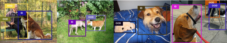
Figure 3: Our methods detect OOD at bounding box level. Images having mixture of in-domain and OOD objects are identified.

As shown in the bottom section of Table 4, none of the single image OOD scores are able to identify the mixed in- and out-domain images, with AUCs between pure and mixed around 0.5.

Table 4: Identifying in-domain and OOD mixed multi-object images using mixture score $g({\bm{x}})$ defined based on different OOD scores. None of the single scores can identify mixed images. New scores based on bounding box detection improve the performance, and our scores outperform the baselines.

		Dog		Bird
		Pure in vs mix	Pure OOD vs mix	Pure in vs mix	Pure OOD vs mix
Scores using bbox	$g(S_{\texttt{sum\_out\_prob}})$	0.6598	0.6918	0.8557	0.7844
	$g(S_{\texttt{-max\_in\_prob}})$ (ours)	0.6836	0.9570	0.7211	0.9833
	$g(S_{\texttt{max\_logit\_diff}})$ (ours)	0.6861	0.8672	0.8846	0.8460
Single score	$S_{\texttt{-max\_prob}}$	0.4907	0.5127	0.4869	0.4787
	$S_{\texttt{sum\_out\_prob}}$	0.5492	0.4940	0.4908	0.4990
	$S_{\texttt{max\_out\_prob}}$	0.5445	0.5152	0.4998	0.4872
	$S_{\texttt{-max\_in\_prob}}$	0.5527	0.5089	0.5169	0.4946
	$S_{\texttt{max\_logit\_diff}}$	0.5794	0.5191	0.4886	0.4639

Image segmentation and object detection are needed for identifying those mixed images. We use Grounding-DINO to localize the multiple objects in bounding boxes along with their confidence scores. Since Grounding-DINO has a limitation on input text length, we decided to use the high level class names for $\mathcal{C}_{\texttt{in}}=${dog} and $\mathcal{C}_{\texttt{out}}=${bird, boat, person, …}. As described in Section 2.4, for each bounding box, we have a list of confidence scores corresponding to the list of class names. Then we compute our proposed OOD scores separately for each bounding box. To find the mixed in-domain and OOD multi-object images, we define the mixture score $g({\bm{x}})$ in Eq. (6) for each image as the greatest score difference among the bounding boxes.

Table 4 shows our proposed mixture score $g({\bm{x}})$, is able to distinguish the mixed images from pure in-domain and pure OOD images, for both dog and bird datasets, having AUCs higher than the baseline.

4 Related work

One-class anomaly detection

Anomaly detection can be formulated as a one-class classification problem [14], which aims to learn the distribution of the normal data only, and then predicts anomalies as data points that are out of the normal distribution. SVM based one-class classification, also called support vector data description (SVDD), fits a hypersphere with the minimum volume that includes most of the normal data points [25]. DeepSVDD leverages the ability of deep neural networks to first learn a good representation before mapping the data to a hypersphere [32]. Later works propose hybrid models that use an autoencoder to learn the data representation, and then map the representation to a one-class classification model [3, 44, 13, 26]. The existing one-class anomaly detection methods have limitations that (1) they need to be trained so they are not zero-shot, (2) they cannot leverage the abnormal data into training, and (3) they are evaluated on simple datasets such as MNIST and CIFAR-10 and on pre-defined closed OOD sets.

Multi-label OOD detection

To the best of our knowledge, all the existing work on multi-label OOD detection is to detect the images that contain none of the in-domain objects [41, 42, 38]. For example, if the in-domain classes are {dog, cat}, the goal is to detect images that do not contain any instances of dogs or cats, such as an image of a chair. In comparison, our work aims to detect the images that contain a mixture of in-domain and OOD objects, such as a dog on a chair. It is challenging to detect the images with mixed in-domain and OOD objects, because the in-domain objects can confound the OOD score. We believe our work is the first to address this problem for in- and out- mixed multi-object out-of-distribution detection.

5 Conclusion and discussion

We propose a novel one-class open-set OOD detector that leverages text-image pre-trained models in a zero-shot fashion and incorporates various descriptions of in-domain and OOD. Unlike prior work, we focus on more challenging and realistic settings for OOD detection. We evaluate on images that are from the long-tail of unseen classes, distribution shifted images, and in-domain and OOD mixed multi-object images. Our method is flexible enough to detect any types of OOD, defined with fine- or coarse-grained labels. Our method shows superior performance over previous baselines on all benchmarks. Nonetheless, our method has room for more improvement. We are interested in additional ways to incorporate natural language to define in-domain and OOD beyond prompts. An additional question is how to effectively use negation to define OOD. Better understanding of the advantages and trade-offs of the proposed two scores is also part of the future work.

Appendix

Tables 5-9 show additional one-class OOD detection results on ImageNet, ImageNet-v2, ImageNet-r, ImageNet-adversarial and ImageNet-Sketch respectively.

We use CLIP ViT-B/16 as the main model for evaluating our method in the main paper. Table 10 shows the ablation study results on ImageNet with ViT-L/14 based CLIP model. Our scores outperformed the baselines on one-class OOD detection tasks, consistent with the main paper’s conclusions.

Table 5: Additional one-class OOD detection results on ImageNet

	$\mathcal{C}_{\texttt{in}}$ vs $\mathcal{C}_{\texttt{out}}$	$\mathcal{C}_{\texttt{in}}^{\prime}$ vs $\mathcal{C}_{\texttt{out}}^{\prime}$
Bird vs non-bird
$S_{\texttt{-max\_prob}}$	0.9827	0.8609
$S_{\texttt{sum\_out\_prob}}$	0.9781	0.8067
$S_{\texttt{max\_out\_prob}}$	0.9943	0.5443
$S_{\texttt{-max\_in\_prob}}$ (ours)	0.9999	0.9912
$S_{\texttt{max\_logit\_diff}}$ (ours)	1.0000	0.9810
Chair vs non-chair
$S_{\texttt{-max\_prob}}$	0.7159	0.3198
$S_{\texttt{sum\_out\_prob}}$	0.9616	0.6338
$S_{\texttt{max\_out\_prob}}$	0.9910	0.7094
$S_{\texttt{-max\_in\_prob}}$ (ours)	0.9967	0.9820
$S_{\texttt{max\_logit\_diff}}$ (ours)	0.9999	0.9785
Cat vs non-cat
$S_{\texttt{-max\_prob}}$	0.7456	0.6732
$S_{\texttt{sum\_out\_prob}}$	0.6262	0.5324
$S_{\texttt{max\_out\_prob}}$	0.9843	0.5554
$S_{\texttt{-max\_in\_prob}}$ (ours)	0.9994	0.9952
$S_{\texttt{max\_logit\_diff}}$ (ours)	1.0000	0.9916

Table 6: Additional one-class OOD detection results on ImageNet-v2

	$\mathcal{C}_{\texttt{in}}$ vs $\mathcal{C}_{\texttt{out}}$	$\mathcal{C}_{\texttt{in}}^{\prime}$ vs $\mathcal{C}_{\texttt{out}}^{\prime}$
Bird vs non-bird
$S_{\texttt{-max\_prob}}$	0.9770	0.8190
$S_{\texttt{sum\_out\_prob}}$	0.9584	0.7855
$S_{\texttt{max\_out\_prob}}$	0.9859	0.5345
$S_{\texttt{-max\_in\_prob}}$ (ours)	0.9989	0.9850
$S_{\texttt{max\_logit\_diff}}$ (ours)	1.0000	0.9745
Chair vs non-chair
$S_{\texttt{-max\_prob}}$	0.8098	0.5739
$S_{\texttt{sum\_out\_prob}}$	0.6639	0.4310
$S_{\texttt{max\_out\_prob}}$	0.9630	0.6300
$S_{\texttt{-max\_in\_prob}}$ (ours)	0.9931	0.9774
$S_{\texttt{max\_logit\_diff}}$ (ours)	0.9978	0.9552
Cat vs non-cat
$S_{\texttt{-max\_prob}}$	0.6488	0.5521
$S_{\texttt{sum\_out\_prob}}$	0.8052	0.5865
$S_{\texttt{max\_out\_prob}}$	0.9909	0.5841
$S_{\texttt{-max\_in\_prob}}$ (ours)	0.9988	0.9937
$S_{\texttt{max\_logit\_diff}}$ (ours)	1.0000	0.9683

Table 7: Additional one-class OOD detection results on ImageNet-r

	$\mathcal{C}_{\texttt{in}}$ vs $\mathcal{C}_{\texttt{out}}$	$\mathcal{C}_{\texttt{in}}^{\prime}$ vs $\mathcal{C}_{\texttt{out}}^{\prime}$
Bird vs non-bird
$S_{\texttt{-max\_prob}}$	0.9346	0.6155
$S_{\texttt{sum\_out\_prob}}$	0.8286	0.5350
$S_{\texttt{max\_out\_prob}}$	0.9820	0.6432
$S_{\texttt{-max\_in\_prob}}$ (ours)	0.9874	0.9528
$S_{\texttt{max\_logit\_diff}}$ (ours)	0.9993	0.9477

Table 8: Additional one-class OOD detection results on ImageNet-adversarial

	$\mathcal{C}_{\texttt{in}}$ vs $\mathcal{C}_{\texttt{out}}$	$\mathcal{C}_{\texttt{in}}^{\prime}$ vs $\mathcal{C}_{\texttt{out}}^{\prime}$
Bird vs non-bird
$S_{\texttt{-max\_prob}}$	0.8647	0.5002
$S_{\texttt{sum\_out\_prob}}$	0.7546	0.5489
$S_{\texttt{max\_out\_prob}}$	0.8896	0.6015
$S_{\texttt{-max\_in\_prob}}$ (ours)	0.9660	0.9212
$S_{\texttt{max\_logit\_diff}}$ (ours)	0.9870	0.9238
Cat vs non-cat
$S_{\texttt{-max\_prob}}$	0.4583	0.6136
$S_{\texttt{sum\_out\_prob}}$	0.5008	0.1434
$S_{\texttt{max\_out\_prob}}$	0.8315	0.3491
$S_{\texttt{-max\_in\_prob}}$ (ours)	0.9951	0.9609
$S_{\texttt{max\_logit\_diff}}$ (ours)	0.9878	0.9009

Table 9: Additional one-class OOD detection results on ImageNet-Sketch

	$\mathcal{C}_{\texttt{in}}$ vs $\mathcal{C}_{\texttt{out}}$	$\mathcal{C}_{\texttt{in}}^{\prime}$ vs $\mathcal{C}_{\texttt{out}}^{\prime}$
Bird vs non-bird
$S_{\texttt{-max\_prob}}$	0.9669	0.6744
$S_{\texttt{sum\_out\_prob}}$	0.8430	0.7789
$S_{\texttt{max\_out\_prob}}$	0.9760	0.5300
$S_{\texttt{-max\_in\_prob}}$ (ours)	0.9900	0.9860
$S_{\texttt{max\_logit\_diff}}$ (ours)	0.9996	0.9845
Chair vs non-chair
$S_{\texttt{-max\_prob}}$	0.8841	0.7309
$S_{\texttt{sum\_out\_prob}}$	0.8091	0.3212
$S_{\texttt{max\_out\_prob}}$	0.9826	0.6285
$S_{\texttt{-max\_in\_prob}}$ (ours)	0.9997	0.9912
$S_{\texttt{max\_logit\_diff}}$ (ours)	1.0000	0.9892
Cat vs non-cat
$S_{\texttt{-max\_prob}}$	0.5086	0.3775
$S_{\texttt{sum\_out\_prob}}$	0.7868	0.3201
$S_{\texttt{max\_out\_prob}}$	0.9571	0.4238
$S_{\texttt{-max\_in\_prob}}$ (ours)	0.9931	0.9915
$S_{\texttt{max\_logit\_diff}}$ (ours)	0.9991	0.9787

Table 10: One-class OOD detection results on ImageNet with ViT-L/14 based CLIP model

	$\mathcal{C}_{\texttt{in}}$ vs $\mathcal{C}_{\texttt{out}}$	$\mathcal{C}_{\texttt{in}}^{\prime}$ vs $\mathcal{C}_{\texttt{out}}^{\prime}$
Dog vs non-dog
$S_{\texttt{-max\_prob}}$	0.9852	0.8802
$S_{\texttt{sum\_out\_prob}}$	0.8684	0.7201
$S_{\texttt{max\_out\_prob}}$	0.9966	0.6640
$S_{\texttt{-max\_in\_prob}}$ (ours)	0.9986	0.9578
$S_{\texttt{max\_logit\_diff}}$ (ours)	1.0000	0.9591
Car vs non-car
$S_{\texttt{-max\_prob}}$	0.8240	0.5324
$S_{\texttt{sum\_out\_prob}}$	0.8368	0.6152
$S_{\texttt{max\_out\_prob}}$	0.9688	0.4115
$S_{\texttt{-max\_in\_prob}}$ (ours)	0.9886	0.9699
$S_{\texttt{max\_logit\_diff}}$ (ours)	0.9989	0.9136
Person vs non-person
$S_{\texttt{-max\_prob}}$	0.7701	0.5207
$S_{\texttt{sum\_out\_prob}}$	0.9873	0.7661
$S_{\texttt{max\_out\_prob}}$	0.9901	0.7458
$S_{\texttt{-max\_in\_prob}}$ (ours)	0.9996	0.5790
$S_{\texttt{max\_logit\_diff}}$ (ours)	1.0000	0.7131
Bird vs non-bird
$S_{\texttt{-max\_prob}}$	0.9825	0.8784
$S_{\texttt{sum\_out\_prob}}$	0.9660	0.6642
$S_{\texttt{max\_out\_prob}}$	0.9944	0.5468
$S_{\texttt{-max\_in\_prob}}$ (ours)	0.9998	0.9644
$S_{\texttt{max\_logit\_diff}}$ (ours)	1.0000	0.9501
Chair vs non-chair
$S_{\texttt{-max\_prob}}$	0.6482	0.3487
$S_{\texttt{sum\_out\_prob}}$	0.9611	0.6423
$S_{\texttt{max\_out\_prob}}$	0.9878	0.6630
$S_{\texttt{-max\_in\_prob}}$ (ours)	0.9969	0.9874
$S_{\texttt{max\_logit\_diff}}$ (ours)	1.0000	0.9828
Cat vs non-cat
$S_{\texttt{-max\_prob}}$	0.8027	0.6915
$S_{\texttt{sum\_out\_prob}}$	0.6384	0.4935
$S_{\texttt{max\_out\_prob}}$	0.9928	0.5705
$S_{\texttt{-max\_in\_prob}}$ (ours)	0.9998	0.9934
$S_{\texttt{max\_logit\_diff}}$ (ours)	1.0000	0.9892

References

- Bitterwolf et al. [2022] Julian Bitterwolf, Alexander Meinke, Maximilian Augustin, and Matthias Hein. Revisiting out-of-distribution detection: A simple baseline is surprisingly effective, 2022. URL https://openreview.net/forum?id=-BTmxCddppP.
- Chalapathy et al. [2017] Raghavendra Chalapathy, Aditya Krishna Menon, and Sanjay Chawla. Robust, deep and inductive anomaly detection. In Machine Learning and Knowledge Discovery in Databases: European Conference, ECML PKDD 2017, Skopje, Macedonia, September 18–22, 2017, Proceedings, Part I 10, pages 36–51. Springer, 2017.
- Chalapathy et al. [2018] Raghavendra Chalapathy, Aditya Krishna Menon, and Sanjay Chawla. Anomaly detection using one-class neural networks. arXiv preprint arXiv:1802.06360, 2018.
- Choi et al. [2018] Hyunsun Choi, Eric Jang, and Alexander A Alemi. WAIC, but why? generative ensembles for robust anomaly detection. arXiv preprint arXiv:1810.01392, 2018.
- Emmott et al. [2015] Andrew Emmott, Shubhomoy Das, Thomas Dietterich, Alan Fern, and Weng-Keen Wong. A meta-analysis of the anomaly detection problem. arXiv preprint arXiv:1503.01158, 2015.
- Esmaeilpour et al. [2022] Sepideh Esmaeilpour, Bing Liu, Eric Robertson, and Lei Shu. Zero-shot out-of-distribution detection based on the pre-trained model CLIP. In Proceedings of the AAAI conference on artificial intelligence, pages 6568–6576, 2022.
- Fort et al. [2021] Stanislav Fort, Jie Ren, and Balaji Lakshminarayanan. Exploring the limits of out-of-distribution detection. Advances in Neural Information Processing Systems, 34:7068–7081, 2021.
- Hendrycks and Gimpel [2016] Dan Hendrycks and Kevin Gimpel. A baseline for detecting misclassified and out-of-distribution examples in neural networks. arXiv preprint arXiv:1610.02136, 2016.
- Hendrycks et al. [2018] Dan Hendrycks, Mantas Mazeika, and Thomas Dietterich. Deep anomaly detection with outlier exposure. arXiv preprint arXiv:1812.04606, 2018.
- Hendrycks et al. [2019a] Dan Hendrycks, Steven Basart, Mantas Mazeika, Andy Zou, Joe Kwon, Mohammadreza Mostajabi, Jacob Steinhardt, and Dawn Song. Scaling out-of-distribution detection for real-world settings. arXiv preprint arXiv:1911.11132, 2019a.
- Hendrycks et al. [2019b] Dan Hendrycks, Kevin Zhao, Steven Basart, Jacob Steinhardt, and Dawn Song. Natural adversarial examples. arXiv preprint arXiv:1907.07174, 2019b.
- Hendrycks et al. [2020] Dan Hendrycks, Steven Basart, Norman Mu, Saurav Kadavath, Frank Wang, Evan Dorundo, Rahul Desai, Tyler Zhu, Samyak Parajuli, Mike Guo, Dawn Song, Jacob Steinhardt, and Justin Gilmer. The many faces of robustness: A critical analysis of out-of-distribution generalization. arXiv preprint arXiv:2006.16241, 2020.
- Hojjati and Armanfard [2021] Hadi Hojjati and Narges Armanfard. DASVDD: Deep autoencoding support vector data descriptor for anomaly detection. arXiv preprint arXiv:2106.05410, 2021.
- Khan and Madden [2010] Shehroz S Khan and Michael G Madden. A survey of recent trends in one class classification. In Artificial Intelligence and Cognitive Science: 20th Irish Conference, AICS 2009, Dublin, Ireland, August 19-21, 2009, Revised Selected Papers 20, pages 188–197. Springer, 2010.
- Kirillov et al. [2023] Alexander Kirillov, Eric Mintun, Nikhila Ravi, Hanzi Mao, Chloe Rolland, Laura Gustafson, Tete Xiao, Spencer Whitehead, Alexander C Berg, Wan-Yen Lo, et al. Segment anything. arXiv preprint arXiv:2304.02643, 2023.
- Lee et al. [2018] Kimin Lee, Kibok Lee, Honglak Lee, and Jinwoo Shin. A simple unified framework for detecting out-of-distribution samples and adversarial attacks. NeurIPS, 2018.
- Li et al. [2022] Daiqing Li, Huan Ling, Seung Wook Kim, Karsten Kreis, Sanja Fidler, and Antonio Torralba. BigDatasetGAN: Synthesizing imagenet with pixel-wise annotations. In Proceedings of the IEEE/CVF Conference on Computer Vision and Pattern Recognition, pages 21330–21340, 2022.
- Liang et al. [2017] Shiyu Liang, Yixuan Li, and R Srikant. Enhancing the reliability of out-of-distribution image detection in neural networks. arXiv preprint arXiv:1706.02690, 2017.
- Liu et al. [2023] Shilong Liu, Zhaoyang Zeng, Tianhe Ren, Feng Li, Hao Zhang, Jie Yang, Chunyuan Li, Jianwei Yang, Hang Su, Jun Zhu, et al. Grounding DINO: Marrying DINO with grounded pre-training for open-set object detection. arXiv preprint arXiv:2303.05499, 2023.
- Liu et al. [2020] Weitang Liu, Xiaoyun Wang, John Owens, and Yixuan Li. Energy-based out-of-distribution detection. Advances in Neural Information Processing Systems, 33:21464–21475, 2020.
- Miller [1995] George A Miller. WordNet: a lexical database for English. Communications of the ACM, 38(11):39–41, 1995.
- Ming et al. [2022] Yifei Ming, Ziyang Cai, Jiuxiang Gu, Yiyou Sun, Wei Li, and Yixuan Li. Delving into out-of-distribution detection with vision-language representations. arXiv preprint arXiv:2211.13445, 2022.
- Morningstar et al. [2021] Warren Morningstar, Cusuh Ham, Andrew Gallagher, Balaji Lakshminarayanan, Alex Alemi, and Joshua Dillon. Density of states estimation for out of distribution detection. In International Conference on Artificial Intelligence and Statistics, pages 3232–3240. PMLR, 2021.
- Nalisnick et al. [2018] Eric Nalisnick, Akihiro Matsukawa, Yee Whye Teh, Dilan Gorur, and Balaji Lakshminarayanan. Do deep generative models know what they don’t know? arXiv preprint arXiv:1810.09136, 2018.
- Noumir et al. [2012] Zineb Noumir, Paul Honeine, and Cedue Richard. On simple one-class classification methods. In 2012 IEEE International Symposium on Information Theory Proceedings, pages 2022–2026. IEEE, 2012.
- Park et al. [2021] JuneKyu Park, Jeong-Hyeon Moon, Namhyuk Ahn, and Kyung-Ah Sohn. What is wrong with one-class anomaly detection? arXiv preprint arXiv:2104.09793, 2021.
- Radford et al. [2021] Alec Radford, Jong Wook Kim, Chris Hallacy, Aditya Ramesh, Gabriel Goh, Sandhini Agarwal, Girish Sastry, Amanda Askell, Pamela Mishkin, Jack Clark, et al. Learning transferable visual models from natural language supervision. In International conference on machine learning, pages 8748–8763. PMLR, 2021.
- Recht et al. [2019] Benjamin Recht, Rebecca Roelofs, Ludwig Schmidt, and Vaishaal Shankar. Do ImageNet classifiers generalize to imagenet? In International Conference on Machine Learning, pages 5389–5400, 2019.
- Ren et al. [2019] Jie Ren, Peter J Liu, Emily Fertig, Jasper Snoek, Ryan Poplin, Mark A DePristo, Joshua V Dillon, and Balaji Lakshminarayanan. Likelihood ratios for out-of-distribution detection. NeurIPS, 2019.
- Ren et al. [2021] Jie Ren, Stanislav Fort, Jeremiah Liu, Abhijit Guha Roy, Shreyas Padhy, and Balaji Lakshminarayanan. A simple fix to Mahalanobis distance for improving near-ood detection. arXiv preprint arXiv:2106.09022, 2021.
- Roy et al. [2022] Abhijit Guha Roy, Jie Ren, Shekoofeh Azizi, Aaron Loh, Vivek Natarajan, Basil Mustafa, Nick Pawlowski, Jan Freyberg, Yuan Liu, Zach Beaver, et al. Does your dermatology classifier know what it doesn’t know? Detecting the long-tail of unseen conditions. Medical Image Analysis, 75:102274, 2022.
- Ruff et al. [2018] Lukas Ruff, Robert Vandermeulen, Nico Goernitz, Lucas Deecke, Shoaib Ahmed Siddiqui, Alexander Binder, Emmanuel Müller, and Marius Kloft. Deep one-class classification. In International conference on machine learning, pages 4393–4402. PMLR, 2018.
- Russakovsky et al. [2015] Olga Russakovsky, Jia Deng, Hao Su, Jonathan Krause, Sanjeev Satheesh, Sean Ma, Zhiheng Huang, Andrej Karpathy, Aditya Khosla, Michael Bernstein, Alexander C. Berg, and Li Fei-Fei. ImageNet Large Scale Visual Recognition Challenge. International Journal of Computer Vision (IJCV), 115(3):211–252, 2015. doi: 10.1007/s11263-015-0816-y.
- Scholkopf et al. [2000] Bernhard Scholkopf, Robert Williamson, Alex Smola, John Shawe-Taylor, John Platt, et al. Support vector method for novelty detection. Advances in neural information processing systems, 12(3):582–588, 2000.
- Shankar* et al. [2020] Vaishaal Shankar*, Rebecca Roelofs*, Horia Mania, Alex Fang, Benjamin Recht, and Ludwig Schmidt. Evaluating machine accuracy on ImageNet. ICML, 2020.
- Sugiyama and Kawanabe [2012] Masashi Sugiyama and Motoaki Kawanabe. Machine learning in non-stationary environments: Introduction to covariate shift adaptation. MIT press, 2012.
- Sun et al. [2022] Yiyou Sun, Yifei Ming, Xiaojin Zhu, and Yixuan Li. Out-of-distribution detection with deep nearest neighbors. arXiv preprint arXiv:2204.06507, 2022.
- Sundar et al. [2020] Vijaya Kumar Sundar, Shreyas Ramakrishna, Zahra Rahiminasab, Arvind Easwaran, and Abhishek Dubey. Out-of-distribution detection in multi-label datasets using latent space of -VAE. In 2020 IEEE Security and Privacy Workshops (SPW), pages 250–255. IEEE, 2020.
- Vasudevan et al. [2022] Vijay Vasudevan, Benjamin Caine, Raphael Gontijo-Lopes, Sara Fridovich-Keil, and Rebecca Roelofs. When does dough become a bagel? Analyzing the remaining mistakes on ImageNet. arXiv preprint arXiv:2205.04596, 2022.
- Wang et al. [2019] Haohan Wang, Songwei Ge, Zachary Lipton, and Eric P Xing. Learning robust global representations by penalizing local predictive power. In Advances in Neural Information Processing Systems, pages 10506–10518, 2019.
- Wang et al. [2021] Haoran Wang, Weitang Liu, Alex Bocchieri, and Yixuan Li. Energy-based out-of-distribution detection for multi-label classification, 2021. URL https://openreview.net/forum?id=KsN9p5qJN3.
- Wang et al. [2022] Lei Wang, Sheng Huang, Luwen Huangfu, Bo Liu, and Xiaohong Zhang. Multi-label out-of-distribution detection via exploiting sparsity and co-occurrence of labels. Image and Vision Computing, 126:104548, 2022.
- Zhai et al. [2022] Xiaohua Zhai, Xiao Wang, Basil Mustafa, Andreas Steiner, Daniel Keysers, Alexander Kolesnikov, and Lucas Beyer. LiT: Zero-shot transfer with locked-image text tuning. In Proceedings of the IEEE/CVF Conference on Computer Vision and Pattern Recognition, pages 18123–18133, 2022.
- Zhang and Deng [2021] Zheng Zhang and Xiaogang Deng. Anomaly detection using improved deep SVDD model with data structure preservation. Pattern Recognition Letters, 148:1–6, 2021.