A Remark on the Uniqueness of Solutions to Hyperbolic Conservation Laws

Abstract

Given a strictly hyperbolic $n\times n$ system of conservation laws, it is well known that there exists a unique Lipschitz semigroup of weak solutions, defined on a domain of functions with small total variation, which are limits of vanishing viscosity approximations. Aim of this note is to prove that every weak solution taking values in the domain of the semigroup, and whose shocks satisfy the Liu admissibility conditions, actually coincides with a semigroup trajectory.

1 Introduction

We consider the Cauchy problem for a strictly hyperbolic $n\times n$ system of conservation laws in one space dimension

$$u_{t}+f(u)_{x}~{}=~{}0,$$ (1.1)

$$u(0,x)~{}=~{}\bar{u}(x),$$ (1.2)

with $f\in{\cal C}^{2}(\mathbb{R}^{n},\mathbb{R}^{n})$. In this setting, it is well known that there exists a Lipschitz continuous semigroup $S:{\cal D}\times[0,+\infty[\,\mapsto{\cal D}$ of weak solutions, defined on a domain ${\cal D}\subset{\bf L}^{1}({\mathbb{R}};\,{\mathbb{R}}^{n})$ of functions with sufficiently small total variation. The trajectories of this semigroup are the unique limits of vanishing viscosity approximations [3]. All of their shocks satisfy the Liu admissibility conditions [2, 17, 18]. We recall that the semigroup is globally Lipschitz continuous w.r.t. the ${\bf L}^{1}$ distance. Namely, there exists a constant $L$ such that

$$\bigl{\|}S_{t}\bar{u}-S_{s}\bar{v}\bigr{\|}_{{\bf L}^{1}}~{}\leq~{}L\Big{(}|t-s|+\|\bar{u}-\bar{v}\|_{{\bf L}^{1}}\Big{)}\qquad\hbox{for all}~{}s,t\geq 0,~{}~{}\bar{u},\bar{v}\in{\cal D}.$$ (1.3)

Given any weak solution $u=u(t,x)$ of (1.1)-(1.2), various conditions have been derived in [7, 9, 10] which guarantee the identity

$$u(t)~{}=~{}S_{t}\bar{u}\qquad\hbox{for all}~{}t\geq 0.$$ (1.4)

Since the semigroup $S$ is unique, the identity (1.4) yields the uniqueness of solutions to the Cauchy problem (1.1)-(1.2). In addition to the standard assumption that each characteristic field is either linearly degenerate or genuinely nonlinear, earlier results required some additional regularity conditions, such as “Tame Variation” or “Tame Oscillation”, controlling the behavior of the solution near a point where the variation is small.

Aim of the present note is to show that uniqueness is guaranteed in a fully general setting: without any assumption about genuine nonlinearity, and without any of the above regularity conditions. Moreover, no assumption is made about the existence of a convex entropy. Our only requirement is that all points of approximate jump satisfy the Liu admissibility conditions.

As in [7, 9, 10], the proof relies on the elementary error estimate

$$\bigl{\|}u(t)-S_{t}\bar{u}\bigr{\|}_{{\bf L}^{1}}~{}\leq~{}L\cdot\int_{0}^{t}\liminf_{h\to 0+}\,{\bigl{\|}u(\tau+h)-S_{h}u(\tau)\bigr{\|}_{{\bf L}^{1}}\over h}\,d\tau\,.$$ (1.5)

Indeed, we will prove that the integrand is zero for a.e. time $\tau\geq 0$. Following an argument introduced in [4], this is achieved by two estimates:

• In a neighborhood of a point $(\tau,y)$ where $u(\tau,\cdot)$ has a large jump, the weak solution $u$ is compared with the solution to a Riemann problem.

• In a region where the total variation is small, the weak solution $u$ is compared with the solution to a linear system with constant coefficients.

To fix ideas, let

$$M~{}\doteq~{}\sup\Big{\{}\mathop{\mathrm{Tot.Var.}}\{\bar{u}\,;{\mathbb{R}}\}\,;~{}~{}\bar{u}\in{\cal D}\Big{\}}$$ (1.6)

be an upper bound for the total variation of all functions in the domain of the semigroup. Notice that this implies

$$\|\bar{u}\|_{{\bf L}^{\infty}}\leq M\qquad\hbox{for all}~{}\bar{u}\in{\cal D}\,.$$ (1.7)

Moreover, for each BV function $\bar{u}\in{\cal D}$, we shall take its right-continuous representative, so that $\bar{u}(x)=\lim_{y\to x+}u(y)$.

To state our result, we first describe the basic setting.

• (Conservation equations) The function $u=u(t,x)$ is a weak solution of the Cauchy problem (1.1)-(1.2) taking values within the domain of the semigroup.
  More precisely, $u:[0,T]\mapsto{\cal D}$ is continuous w.r.t. the ${\bf L}^{1}$ distance. The identity $u(0,\cdot)=\bar{u}$ holds in ${\bf L}^{1}$, and moreover

  $$\int\!\!\int\big{(}u\varphi_{t}+f(u)\varphi_{x}\big{)}~{}dxdt=0$$ (1.8)

  for every ${\cal C}^{1}$ function $\varphi$ with compact support contained inside the open strip $\,]0,T[\,\times{\mathbb{R}}$.

To introduce the Liu admissibility condition on the shocks [17, 18], we first recall that (A1) implies that $u=u(t,x)$ is a function of bounded variation in time and space (cf. [15, Section 5.1] for the definition). Indeed, by [13, Theorem 4.3.1], we have the Lipschitz bound

$$\bigl{\|}u(t_{2},\cdot)-u(t_{1},\cdot)\bigr{\|}_{{\bf L}^{1}({\mathbb{R}})}~{}\leq~{}C_{M}\,(t_{2}-t_{1})\qquad\qquad\hbox{for all}~{}0\leq t_{1}\leq t_{2}\,,$$ (1.9)

for some constant $C_{M}>0$ depending only on the flux $f$ and on the upper bound $M$ for the total variation.

By the structure theorem for BV functions of two variables (see e.g. [15, Section 5.9] or [1]), there is a Borel subset $\mathbf{J}\subset[0,1]\times\mathbb{R}$ with the following three properties.

• Every point $(\tau,\xi)\not\in\mathbf{J}$ is a point of approximate continuity.

• $\mathbf{J}$ is countably $1$-rectifiable, i.e. it can be covered by countably many Lipschitz curves, possibly leaving out a subset of zero $\mathcal{H}^{1}$ measure ($\mathcal{H}^{1}$ denotes the Hausdorff $1$-dimensional measure, cf. [15, Section 2.1]).

• $\mathcal{H}^{1}$-almost every point $(\tau,\xi)\in\mathbf{J}$ is an approximate jump of the function $u$. More precisely there exist states $u^{-},u^{+}\in{\mathbb{R}}^{n}$ and a speed $\lambda\in{\mathbb{R}}$ such that, calling

  $$U(t,x)~{}\doteq~{}\left\{\begin{array}[]{rl}u^{-}&\hbox{if}\qquad x<\lambda t,\\[2.84526pt] u^{+}&\hbox{if}\qquad x>\lambda t,\end{array}\right.$$ (1.10)

  there holds

  $$\lim_{r\to 0+}~{}{1\over r^{2}}\int_{-r}^{r}\int_{-r}^{r}\Big{|}u(\tau+t,~{}\xi+x)-U(t,x)\Big{|}~{}dx\,dt~{}=~{}0.$$ (1.11)

Defining the rescaled functions

$$u_{r}(t,x)\,\doteq\,u(\tau+rt,\xi+rx)\,,$$ (1.12)

by (iii) and (A1) it follows that $u_{r}$ converges to $U$ in ${\bf L}^{1}_{loc}({\mathbb{R}}^{2})$. In particular the conservation equations (1.8) must hold for the piecewise constant function $U$, and the triple $(u^{+},u^{-},\lambda)$ must therefore satisfy the Rankine-Hugoniot equations:

$$f(u^{+})-f(u^{-})~{}=~{}\lambda(u^{+}-u^{-}).$$ (1.13)

Now let a left state $u^{-}\in{\mathbb{R}}^{n}$ be given. Since the system is strictly hyperbolic, there exist $n$ shock curves

$$s\mapsto S_{i}(s)(u^{-}),\qquad\qquad i=1,\ldots,n,$$

parameterizing the sets of right states $u^{+}$ connected to the left state $u^{-}$ by a shock of the $i$-th family [5, 13, 16]. As in (1.13), denote by $\lambda=\lambda_{i}(s)$ the Rankine-Hugoniot speed of a shock with left and right states $u^{-}$ and $u^{+}=S_{i}(s)(u^{-})$,

• (Liu admissibility condition) In the above setting, a shock with left and right states $u^{-}$ and $u^{+}=S_{i}(\sigma)(u^{-})$ is Liu-admissible if $\lambda_{i}(\sigma)\leq\lambda_{i}(s)$ for all $s\in[0,\sigma]$.

Our result can be simply stated as:

Theorem 1.1.

Let (1.1) be a strictly hyperbolic $n\times n$ system. Then every weak solution $u:[0,T]\mapsto{\cal D}$, taking values within the domain of the semigroup and whose shocks satisfy the Liu admissibility condition, coincides with a semigroup trajectory.

Under the additional assumptions that each characteristic family is either linearly degenerate or genuinely nonlinear, and that the $n\times n$ system (1.1) admits a strictly convex entropy selecting the admissible shocks, this uniqueness result was recently proved in [8]. Restricted to a class of $2\times 2$ systems, an earlier proof can also be found in [12].

2 Proof of the theorem

1. Let $\mathbf{J}$ be the set introduced in the previous section and let $\mathbf{S}\subset\mathbf{J}$ be the subset of all points which are not approximate jumps. Since $\mathcal{H}^{1}(\mathbf{S})=0$, its projection on the time axis is a subset ${\cal N}\subset[0,T]$ which is null for the Lebesgue measure. Every point $(t,x)\in[0,T]\times{\mathbb{R}}$ with $t\notin{\cal N}$ is therefore either a point of approximate jump, or a point of approximate continuity.

Let us denote by ${\cal J}$ the set

$${\cal J}\,\doteq\,\bigl{\{}(\tau,\xi):\tau\not\in{\cal N}\;\mbox{and $(\tau,\xi)$ is an approximate jump}\bigr{\}}\,.$$

While it follows immediately from the aforementioned BV structure theorem that ${\cal J}$ is rectifiable, we claim here a stronger property: ${\cal J}$ can be covered by the graphs of countably many Lipschitz functions

$$x=\phi_{\ell}(t),\qquad\qquad\ell\in{\mathbb{N}}\,,$$ (2.1)

and moreover the Lipschitz constant of each $\phi_{\ell}$ is bounded by a number $\Lambda$ which depends only on $f$ and on the constant $M$ in (1.6). More precisely, by recalling (1.7) we can set

$$\Lambda~{}\doteq~{}2\,{\rm Lip}\bigl{(}f,B_{M}\bigr{)},$$ (2.2)

where the right hand side denotes the Lipschitz constant of the function $f$ over the ball $B_{M}\subset{\mathbb{R}}^{n}$ centered at the origin with radius $M$.

Since by (1.7) it follows

$$|u^{\pm}(\tau,\xi)|\leq M\qquad\hbox{for all}~{}(\tau,\xi)\in{\cal J},$$

the above definition implies that the shock speed $\lambda=\lambda(\tau,\xi)$ at (1.10), (1.13) satisfies the bound

$$|\lambda(\tau,\xi)|~{}\leq~{}{\rm Lip}\,(f,B_{M})~{}\leq~{}\frac{\Lambda}{2}\,.$$ (2.3)

In order to prove our claim, we decompose $\cal J$ in the countable union of suitable pieces. First of all, for every integer $k\geq 1$ we define

$${\cal J}_{k}~{}\doteq~{}\left\{(\tau,\xi)\in{\cal J}:|u^{+}(\tau,\xi)-u^{-}(\tau,\xi)|\geq\frac{1}{k}\right\}.$$

Obviously, ${\cal J}=\bigcup_{k}{\cal J}_{k}$. Next, given any pairs $(\tau_{1},\xi_{1})$ and $(\tau_{2},\xi_{2})$ in ${\cal J}_{k}$, consider the two piecewise constant functions

$$U_{j}(t,x)~{}\doteq~{}\left\{\begin{array}[]{rl}u^{-}(\tau_{j},\xi_{j})&\hbox{if}\qquad x<\lambda(\tau_{j},\xi_{j})t,\\[5.69054pt] u^{+}(\tau_{j},x_{j})&\hbox{if}\qquad x>\lambda(\tau_{j},\xi_{j})t,\end{array}\right.\qquad\qquad j=1,2.$$ (2.4)

By (2.3) there is a positive number $\varepsilon(k,\Lambda)$ depending on $k$ and $\Lambda$ such that the following holds. If $(\tau_{s},\xi_{s})$ is yet a third point in the plane with the properties that $\tau_{s}^{2}+\xi_{s}^{2}=1$ and $|\xi_{s}|\geq\Lambda|\tau_{s}|$, then if we “shift” $U_{2}$ by this vector we get the inequality

$$\int_{B_{1}}\bigl{|}U_{1}(t,x)-U_{2}(t+\tau_{s},x+\xi_{s})\bigr{|}\,dx\,dt~{}\geq~{}6\varepsilon\,,$$ (2.5)

where $B_{1}$ denotes the unit disk centered at the origin in $\mathbb{R}^{2}$. We subdivide further ${\cal J}_{k}$ as a union of sets ${\cal J}_{k,j}$, $j\geq 1$, where $(\tau,\xi)$ belongs to ${\cal J}_{k,j}$ if

$$\int_{B_{r}(\tau,\xi)}|u(t,x)-U(t-\tau,x-\xi)|\,dx\,dt\leq\varepsilon r^{2}\qquad\hbox{for all}~{}r<\frac{1}{j}\,.$$ (2.6)

Here $U$ is defined as in (1.10) and $B_{r}(\tau,\xi)$ denotes the disk centered at $(\tau,\xi)$ with radius $r$. Clearly,

$${\cal J}~{}=~{}\bigcup_{k}{\cal J}_{k}~{}=~{}\bigcup_{k,j}{\cal J}_{k,j}\,.$$

Next, consider two points $(\tau_{1},\xi_{1}),(\tau_{2},\xi_{2})\in{\cal J}_{k,j}$ such that $r\doteq\bigl{|}(\tau_{1},\xi_{1})-(\tau_{2},\xi_{2})\bigr{|}<\frac{1}{2j}$. Let $U_{j}$ be as in (2.4) and set the shift $(\tau_{s},\xi_{s})$ to be

$$\tau_{s}\,=\,\frac{\tau_{1}-\tau_{2}}{r}\,,\qquad\quad\xi_{s}\,=\,\frac{\xi_{1}-\xi_{2}}{r}\,.$$

We claim that (2.5) cannot hold with this shift. This will enable us to conclude $|\xi_{s}|\leq\Lambda|\tau_{s}|$. To prove the claim, observe first that

$$\int_{B_{1}}|U_{1}(t,x)-U_{2}(t+\tau_{s},x+\xi_{s})|\,dx\,dt$$

$$\leq \int_{B_{1}}|U_{1}(t,x)-u(\tau_{1}+rt,\xi_{1}+rx)|\,dx\,dt+\int_{B_{1}}|u(\tau_{1}+rt,\xi_{1}+rx)-U_{2}(t+\tau_{s},x+\xi_{s})|\,dx\,dt$$

We then change variables in the integrals to $(\sigma,y)=(\tau_{1}+rt,\xi_{1}+rx)$. Observe that

$$\begin{array}[]{rl}t+\tau_{s}&=~{}t+r^{-1}(\tau_{1}-\tau_{2})~{}=~{}r^{-1}(t+\tau_{1}-\tau_{2})=r^{-1}(\sigma-\tau_{2}),\\[2.84526pt] x+\xi_{s}&=~{}x+r^{-1}(\xi_{1}-\xi_{2})~{}=~{}r^{-1}(y-\xi_{2}),\end{array}$$

while $U_{j}\bigl{(}r^{-1}(\sigma-\tau_{j}),r^{-1}(y-\xi_{j})\bigr{)}=U_{j}(\sigma-\tau_{j},y-\xi_{j})$ because of the $0$-homogeneity of the functions $U_{j}$. Hence the change of variables yields

$$\begin{array}[]{l}\displaystyle\int_{B_{1}}\bigl{|}U_{1}(t,x)-U_{2}(t+\tau_{s},x+\xi_{s})\bigr{|}\,dx\,dt\\[11.38109pt] \qquad\qquad\qquad\leq~{}\displaystyle\frac{1}{r^{2}}\int_{B_{r}(\tau_{1},\xi_{1})}\bigl{|}U_{1}(\sigma-\tau_{1},y-\xi_{1})-u(\sigma,y)\bigr{|}\,dy\,d\sigma\\[11.38109pt] \qquad\qquad\qquad\qquad\qquad\qquad\qquad\displaystyle+\frac{1}{r^{2}}\int_{B_{r}(\tau_{1},\xi_{1})}\bigl{|}u(\sigma,y)-U_{2}(\sigma-\tau_{2},y-\xi_{2})\bigr{|}\,dy\,d\sigma\\[11.38109pt] \displaystyle\qquad\qquad\qquad\leq~{}\frac{1}{r^{2}}\int_{B_{r}(\tau_{1},\xi_{1})}\bigl{|}U_{1}(\sigma-\tau_{1},y-\xi_{1})-u(\sigma,y)\bigr{|}\,dy\,d\sigma\\[11.38109pt] \qquad\qquad\qquad\qquad\qquad\qquad\qquad\displaystyle+\frac{1}{r^{2}}\int_{B_{2r}(\tau_{2},\xi_{2})}\bigl{|}u(\sigma,y)-U_{2}(\sigma-\tau_{2},y-\xi_{2})\bigr{|}\,dy\,d\sigma,\end{array}$$

where we have used the inclusion $B_{r}(\tau_{1},\xi_{1})\subset B_{2r}(\tau_{2},\xi_{2})$ to get the last inequality. Note next that $r<2r<\frac{1}{j}$ and, since both $(\tau_{1},\xi_{1})$ and $(\tau_{2},\xi_{2})$ belong to ${\cal J}_{k,j}$, we can use (2.6) to bound the first summand by $\varepsilon$ and the second summand by $4\varepsilon$. In particular we conclude

$$\int_{B_{1}}\bigl{|}U_{1}(t,x)-U_{2}(t+\tau_{s},x+\xi_{s})\bigr{|}\,dx\,dt\leq 5\varepsilon\,.$$

As already pointed out, since the latter inequality contradicts (2.5), we conclude that $|\xi_{s}|\leq\Lambda|\tau_{s}|$, which in turn gives $|\xi_{2}-\xi_{1}|\leq\Lambda|\tau_{2}-\tau_{1}|$.

We have thus proved the following fact:

• If $(\tau_{1},\xi_{1}),(\tau_{2},\xi_{2})\in{\cal J}_{k,j}$ and $|(\tau_{1},\xi_{1})-(\tau_{2},\xi_{2})|<\frac{1}{2j}$, then $|\xi_{2}-\xi_{1}|\leq\Lambda|\tau_{2}-\tau_{1}|$.

It is well known that from (L) it follows that ${\cal J}_{k,j}$ can be covered by countably many Lipschitz graphs of functions $x=\phi_{\ell}(t)$, $\ell\in\mathbb{N}$, with Lipschitz constant at most $\Lambda$. See for instance [14, Lemma 4.7].

For readers’ convenience, we include here a proof. If $B=B_{1/{4j}}(x_{0},t_{0})$ is any disk of radius $1/(4j)$ and we set $F\doteq{\cal J}_{k,j}\cap B$, then (L) implies

$$|x-y|\leq\Lambda|t-s|\qquad\hbox{for all}~{}(t,x),(s,y)\in F\,.$$ (2.7)

This obviously implies that there are no points of $F$ which lie on the same line $\{t={\rm const}\}$. Hence, if $G$ is the projection of $F$ on the time axis, then there is a function $\phi:G\to\mathbb{R}$ such that $F=\{(t,\phi(t)):t\in G\}$. On the other hand (2.7) is equivalent to the statement that the Lipschitz constant of $G$ is at most $\Lambda$. By the classical Lipschitz extension theorem we can simply extend $\phi$ to a Lipschitz function defined on the whole time axis. Since ${\cal J}_{k,j}$ can be covered by a countable collection of disks with radius $1/(4j)$, the existence of the desired covering by means of countably many Lipschitz graphs follows immediately. 2. Next, we wish to show that, if $t\not\in{\cal N}$ and $(t,x)\not\in\mathbf{J}$, then $y\mapsto u(t,y)$ is continuous at $x$. We start by noticing that, since $(t,x)\not\in\mathbf{J}$, $u$ is approximately continuous at $(t,x)$ as a function of two variables. Therefore there is a $u_{0}\in\mathbb{R}^{n}$ such that

$$\lim_{r\downarrow 0}\frac{1}{r^{2}}\int_{t-r}^{t+r}\int_{x-r}^{x+r}|u(s,y)-u_{0}|\,ds\,dy~{}=~{}0\,.$$

In particular, for every fixed $\varepsilon>0$ there is an $r_{0}(\varepsilon)>0$ such that

$$\int_{t-r}^{t+r}\int_{x-r}^{x+r}|u(s,y)-u_{0}|\,ds\,dy~{}\leq~{}\varepsilon r^{2}\qquad\hbox{for all}~{}r\leq r_{0}(\varepsilon)\,.$$

An elementary application of Chebyshev’s inequality and Fubini’s theorem yields then the existence of a $t(r)\in[t-r\sqrt{\varepsilon},t+r\sqrt{\varepsilon}]$ such that

$$\int_{x-r}^{x+r}|u(t(r),y)-u_{0}|\,dy~{}\leq~{}r\sqrt{\varepsilon}\,.$$

Furthermore we can use the Lipschitz estimate (1.9) to bound

$$\frac{1}{r}\int_{x-r}^{x+r}|u(t,y)-u_{0}|\,dy\leq\sqrt{\varepsilon}+C_{M}\frac{|t-t(r)|}{r}~{}\leq~{}(1+C_{M})\sqrt{\varepsilon}\qquad\hbox{for all}~{}r\leq r_{0}(\varepsilon)\,.$$ (2.8)

On the other hand recall that $y\mapsto u(t,y)$ is a function of bounded variation on the real line. As such, every point is either a classical jump point, or a point of continuity. Since $\varepsilon$ in (2.8) can be closen arbitrarily small, $x$ cannot be a classical jump point of $u(t,\cdot)$ and must therefore be a point of continuity, which was in fact our initial claim. 3. Together with the functions $\phi_{\ell}$ in (2.1), we consider functions of the form

$$\phi^{y+}(t)=y+\Lambda t,\qquad\qquad\phi^{y-}(t)=y-\Lambda t,\qquad\qquad y\in{\mathbb{Q}}.$$ (2.9)

Since here $y$ is a rational point, there are countably many of these functions. For convenience, the countable set of all functions in (2.1) together with those in (2.9) will be relabeled as

$$\{\psi_{n}\,;~{}~{}n\geq 1\}.$$ (2.10)

Next, we observe that, for every $j,k\geq 1$, the scalar function

$$W_{jk}(t)~{}\doteq~{}\left\{\begin{array}[]{cl}\mathop{\mathrm{Tot.Var.}}\big{\{}u(t)\,;~{}]\psi_{j}(t)\,,~{}\psi_{k}(t)[\,\bigr{\}}&\hbox{if}\quad\psi_{j}(t)<\psi_{k}(t)\,,\\[5.69054pt] 0&\hbox{otherwise,}\end{array}\right.$$ (2.11)

is bounded and measurable (indeed, it is lower semicontinuous). Therefore a.e. $t\in[0,T]$ is a Lebesgue point. We denote by ${\cal N}^{\prime}\subset[0,T]$ the set of all times $t$ which are NOT Lebesgue for at least one of the countably many functions $W_{jk}$. Of course, ${\cal N}^{\prime}$ has zero Lebesgue measure.

In view of (1.5), we will prove the theorem by establishing the following claim.

• For every $\tau\in[0,T]\setminus({\cal N\cup\cal N^{\prime}})$ and $\varepsilon>0$, one has

  $$\limsup_{h\to 0+}{1\over h}\Big{\|}u(\tau+h)-S_{h}u(\tau)\Big{\|}_{{\bf L}^{1}}~{}\leq~{}\varepsilon.$$ (2.12)

4. Assume $\tau\notin\cal N\cup\cal N^{\prime}$. By induction on $k=0,1,2,\ldots,N$, we will construct points

$$y_{0}\leq y_{0}^{\prime}~{}<~{}y_{1}\leq y^{\prime}_{1}~{}<~{}y_{2}\leq y^{\prime}_{2}~{}<~{}\cdots~{}<~{}y_{N}\leq y_{N}^{\prime}$$

with the following properties.

• Either $y_{k}=y_{k}^{\prime}=\phi_{j}(\tau)$ for some $j$, or else $y_{k}<y^{\prime}_{k}$ and

  $$y_{k}^{\prime}+\Lambda\tau\in{\mathbb{Q}},\qquad\qquad y_{k}-\Lambda\tau\in{\mathbb{Q}}\,.$$ (2.13)

• The first and the last points satisfy

  $$\mathop{\mathrm{Tot.Var.}}\bigl{\{}u(\tau,\cdot)\,;~{}]-\infty,\,y_{0}^{\prime}[\,\bigr{\}}~{}<~{}\varepsilon,$$ (2.14)

  $$\mathop{\mathrm{Tot.Var.}}\bigl{\{}u(\tau,\cdot)\,;~{}]y_{N},\,+\infty[\,\bigr{\}}~{}<~{}\varepsilon.$$ (2.15)

  Moreover, for every $k\in\{1,\ldots,N\}$, considering the total variation of the right-continuous function $u(\tau,\cdot)$ on the following open and half-open intervals, one has

  $$\mathop{\mathrm{Tot.Var.}}\bigl{\{}u(\tau,\cdot)\,;~{}]y_{k-1},\,y_{k}^{\prime}[\,\,\bigr{\}}~{}<~{}2\varepsilon,$$ (2.16)

  $$\mathop{\mathrm{Tot.Var.}}\bigl{\{}u(\tau,\cdot)\,;~{}]y_{k-1},\,y_{k}^{\prime}]\,\bigr{\}}~{}>~{}\varepsilon,$$ (2.17)

  $$\mathop{\mathrm{Tot.Var.}}\bigl{\{}u(\tau,\cdot)\,;~{}]y_{k},\,y_{k}^{\prime}]\,\,\bigr{\}}~{}<~{}{\varepsilon\over 2}\,.$$ (2.18)

The construction is straightforward. We first determine points $y_{0}<y_{0}^{\prime}$ satisfying (2.13) and such that (2.14) holds together with

$$\mathop{\mathrm{Tot.Var.}}\bigl{\{}u(\tau,\cdot)\,;~{}]y_{0}\,,\,y_{0}^{\prime}]\,\bigr{\}}~{}<~{}{\varepsilon\over 2}\,.$$

Next, assume by induction that the points $y_{0},\ldots y_{k-1},y_{k-1}^{\prime}$ have already been constructed. Consider the point

$$z_{k}~{}=~{}\sup~{}\Big{\{}x>y_{k-1}^{\prime}\,;~{}~{}\mathop{\mathrm{Tot.Var.}}\bigl{\{}u(\tau,\cdot)\,;~{}~{}]y_{k-1},x[\,\bigr{\}}<{3\varepsilon\over 2}\Big{\}}.$$

CASE 1: If the map $y\mapsto u(\tau,y)$ has a jump at $z_{k}$, then by step 2 we have $(\tau,z_{k})\in{\bf J}$. Hence by step 1 it follows $z_{k}=\phi_{j}(\tau)$ for some $j$. In this case we set $y_{k}=y_{k}^{\prime}=z_{k}$. CASE 2: If the map $y\mapsto u(\tau,y)$ is continuous at $z_{k}$, then we can take two points $y_{k}<z_{k}<y_{k}^{\prime}$ such that (2.13) holds, together with (2.16)–(2.18). Since $\mathop{\mathrm{Tot.Var.}}\bigl{\{}u(\tau,\cdot)\bigr{\}}\leq M$, by (2.17) the total number of points $y_{k}$ will be

$$N~{}\leq~{}{2M\over\varepsilon}\,.$$ (2.19)

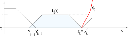
Figure 1: The points $y_{k}$, $y_{k}^{\prime}$ constructed in the proof of the theorem.

5. The remainder of the proof is very similar to the one in [8]. For any given $y\in{\mathbb{R}}$, we denote by $U^{\sharp}=U^{\sharp}_{(u,\tau,y)}(t,x)$ the solution to the Riemann problem for (1.1), with initial data

$$u(\tau,x)~{}=~{}\left\{\begin{array}[]{rl}u(\tau,y-)&\hbox{if}~{}~{}x<y,\cr u(\tau,y+)&\hbox{if}~{}~{}x>y.\end{array}\right.$$ (2.20)

Moreover, for every given $k\geq 1$ we denote by $U^{\flat}=U^{\flat}_{(u,\tau,k)}(t,x)$ the solution to the linear Cauchy problem with constant coefficients

$$v_{t}+Av_{x}~{}=~{}0,\qquad\qquad v(\tau,x)=u(\tau,x).$$ (2.21)

Here the $n\times n$ matrix $A$ is the Jacobian matrix of $f$ computed at the midpoint of the interval $[y_{k-1},y^{\prime}_{k}]$. Namely,

$$A~{}=~{}Df\left(u\Big{(}\tau,{y_{k-1}+y^{\prime}_{k}\over 2}\Big{)}\right).$$

With reference to Fig. 1, to estimate the lim-sup in (2.12), we need to estimate two types of integrals.

• The integral of $\bigl{|}u(t,x)-U^{\sharp}_{(u,\tau,y_{k})}(t,x)\bigr{|}$ over the intervals

  $$J_{y}(t)~{}\doteq~{}\bigl{[}y_{k}-\Lambda(t-\tau)\,,~{}y_{k}+\Lambda(t-\tau)\bigr{]},$$

  for every $k$ such that $y_{k}=y_{k}^{\prime}$.

• The integral of $\bigl{|}u(t,x)-U^{\flat}_{(u,\tau,k)}(t,x)\bigr{|}$ over the intervals

  $$J_{k}(t)~{}=~{}\bigl{[}y_{k-1}+\Lambda(t-\tau)\,,~{}y_{k}^{\prime}-\Lambda(t-\tau)\bigr{]}.$$

6. To estimate integrals of type (I) we observe that, since $\tau\notin{\cal N}$, $(\tau,y_{k})$ is either a Lebesgue point or a point of approximate jump of the function $u$. Therefore

$$\lim_{t\to\tau+}~{}{1\over t-\tau}\int_{y_{k}-\Lambda(t-\tau)}^{y_{k}+\Lambda(t-\tau)}\Big{|}u(t,x)-U^{\sharp}_{(u;\tau,y_{k})}(t,x)\Big{|}~{}dx~{}=~{}0.$$ (2.22)

Indeed, this follows from (1.11) and the Lipschitz continuity of the map $t\mapsto u(t,\cdot)\in{\bf L}^{1}({\mathbb{R}})$. See Theorem 2.6 in [5] for details. 7. To estimate integrals of type (II), two main cases will be considered.

CASE 1: $y_{k-1}-\Lambda\tau\in{\mathbb{Q}}$ and $y^{\prime}_{k}+\Lambda\tau\in{\mathbb{Q}}$. In this case, since $\tau\notin{\cal N}^{\prime}$, the function

$$V(t)~{}\doteq~{}\mathop{\mathrm{Tot.Var.}}\Big{\{}u(t,\cdot)\,;~{}\bigl{]}y_{k-1}+\Lambda(t-\tau)\,,~{}y^{\prime}_{k}-\Lambda(t-\tau)\bigr{[}\Big{\}}$$ (2.23)

has a Lebesgue point at $t=\tau$. Hence

$$\lim_{h\to 0+}{1\over h}\int_{\tau}^{\tau+h}\bigl{|}V(t)-V(\tau)\bigr{|}\,dt~{}=~{}0.$$

Since $V(\tau)\leq 2\varepsilon$, this implies

$$\limsup_{h\to 0+}{1\over h}\int_{\tau}^{\tau+h}V(t)\,dt~{}\leq~{}2\varepsilon.$$ (2.24)

CASE 2: $y_{k-1}=\phi_{\ell}(\tau)$, $y^{\prime}_{k}=\phi_{\ell^{\prime}}(\tau)$ for some indices $\ell,\ell^{\prime}\in{\mathbb{N}}$. In this case, since $\tau\notin{\cal N}^{\prime}$, the function

$$W(t)~{}\doteq~{}\mathop{\mathrm{Tot.Var.}}\Big{\{}u(t,\cdot)\,;~{}\bigl{]}\phi_{\ell}(t)\,,~{}\phi_{\ell^{\prime}}(t)\bigr{[}\Big{\}}$$

has a Lebesgue point at $t=\tau$. Recalling that the functions $\phi_{\ell}$, $\phi_{\ell^{\prime}}$ have Lipschitz constant $\leq\Lambda$, a comparison with (2.23) immediately yields $V(t)\leq W(t)$ for all $t\geq\tau$. Since our construction implies $W(\tau)\leq 2\varepsilon$, we thus conclude that (2.24) again holds.

The remaining two cases, where $y_{k-1}=\phi_{\ell}(\tau)$ and $y^{\prime}_{k}+\Lambda\tau\in{\mathbb{Q}}$, or where $y_{k-1}-\Lambda\tau\in{\mathbb{Q}}$ and $y^{\prime}_{k}=\phi_{\ell^{\prime}}(\tau)$ for some $\ell,\ell^{\prime}\in{\mathbb{N}}$, can be handled in the same way. Namely, (2.24) always holds. Using again the fact that the map $t\mapsto u(t,\cdot)$ is Lipschitz continuous from $[0,T]$ into ${\bf L}^{1}({\mathbb{R}})$, the same argument used in [8] now yields

$$\limsup_{t\to\tau+}\frac{1}{t-\tau}\int_{y_{k-1}+\Lambda(t-\tau)}^{y_{k}^{\prime}-\Lambda(t-\tau)}\left|u(t,x)-U^{\flat}_{(u,\tau,k)}\left(t,x\right)\right|\;dx~{}=~{}{\cal O}(1)\cdot\varepsilon^{2}.$$ (2.25)

Indeed, this corresponds to formula (3.20) in [8]. Based on (2.24), the proof is identical and will not be repeated here. 8. On the other hand, as showed in [3] all trajectories of the semigroup are weak solutions of (1.1) which satisfy the Liu admissibility conditions. Therefore they satisfy the same bounds as in (2.22) and (2.25). More precisely:

$$\lim_{t\to\tau+}{1\over t-\tau}\int_{y_{k}-\Lambda(t-\tau)}^{y_{k}+\Lambda(t-\tau)}\Big{|}\bigl{(}S_{t-\tau}u(\tau)\bigr{)}(x)-U^{\sharp}_{(u;\tau,y_{k})}(t,x)\Big{|}~{}dx~{}=~{}0,$$ (2.26)

$$\limsup_{t\to\tau+}\frac{1}{t-\tau}\int_{y_{k-1}+\Lambda(t-\tau)}^{y_{k}^{\prime}-\Lambda(t-\tau)}\Big{|}\bigl{(}S_{t-\tau}u(\tau)\bigr{)}(x)-U^{\flat}_{(u,\tau,k)}(t,x)\Big{|}~{}dx~{}=~{}{\cal O}(1)\cdot\varepsilon^{2}.$$ (2.27)

9. Combining the previous estimates (2.22), (2.25), (2.26), (2.27), and recalling that the total number of intervals is $N\leq 2M\varepsilon^{-1}$, we establish the limit (2.12), proving the theorem. MM     

Acknowledgments. The research by the first author was partially supported by NSF with grant DMS-2006884, “Singularities and error bounds for hyperbolic equations”.

References

[1] L. Ambrosio, N. Fusco, and D. Pallara,
Functions of Bounded Variation and Free Discontinuity Problems.
Clarendon Press, Oxford, 2000.
[2]
S. Bianchini,
On the Riemann problem for non-conservative hyperbolic systems.
Arch. Rational Mech. Anal.166 (2003), 1–26.
[3] S. Bianchini and A. Bressan, Vanishing viscosity solutions
of nonlinear hyperbolic systems, Annals of Math.161
(2005), 223–342.
[4] A. Bressan,
The unique limit of the Glimm scheme, Arch. Rational
Mech. Anal.130 (1995), 205–230.
[5]
A. Bressan, Hyperbolic Systems of Conservation Laws. The One
Dimensional Cauchy Problem. Oxford University Press, 2000.
[6] A. Bressan, G. Crasta, and B. Piccoli, Well posedness of
the Cauchy problem for systems of conservation laws,
Amer. Math. Soc. Memoir694 (2000).
[7] A. Bressan and P. Goatin,
Oleinik type estimates and uniqueness for
conservation laws, J. Differential Equations156 (1999), 26–49.
[8] A. Bressan and G. Guerra,
Unique solutions to hyperbolic conservation laws with a strictly convex entropy, preprint,
http://arxiv.org/abs/2305.10737
[9] A. Bressan and P. LeFloch, Uniqueness of weak solutions to systems of conservation laws,
Arch. Rational Mech. Anal.140 (1997), 301–317.
[10] A. Bressan and M. Lewicka, A uniqueness condition for hyperbolic systems of conservation laws, Discr. Cont. Dyn. Syst.6 (2000), 673–682.
[11] A. Bressan, T. P. Liu and T. Yang, stability
estimates for conservation laws,
Arch. Rational Mech. Anal.149 (1999), 1–22.
[12] G. Chen, S. Krupa, and A. Vasseur,
Uniqueness and weak-BV stability for 2x2 conservation laws,
Arch. Rational Mech. Anal.246 (2022), 299–332.
[13] C. Dafermos
Hyperbolic Conservation Laws in Continuum
Physics. 4-th Edition, Springer, 2016.
[14] C. De Lellis, Rectifiable sets, Densities, and Tangent Measures.
Zurich Lectures in Advanced Mathematics. European Mathematical Society, Zurich, 2008.
[15]
L. C. Evans and R. F. Gariepy,
Measure Theory and Fine Properties of Functions.
CRC Press, 1991.
[16]
H. Holden and N.H. Risebro,
Front Tracking for Hyperbolic Conservation Laws. Springer, 2015.
[17] T. P. Liu, Riemann problem for general conservation laws.
Trans. Amer. Math. Soc.199 (1974), 89–112.
[18] T. P. Liu, The entropy condition and the admissibility of shocks.
J. Math. Anal. Appl. 53 (1976), 78–88.