Impact of central mixing scheme and nuclear reaction network on the extent of convective cores

Convective cores are the hydrogen reservoirs of main sequence stars that are more massive than around 1.2 solar masses. The characteristics of the cores have a strong impact on the evolution and structure of the star. However, such results rely on stellar evolution codes, in which simplistic assumptions are often made on the physics in the core. Indeed, mixing is commonly considered to be instantaneous and the most basic nuclear networks assume beryllium at its equilibrium abundance. Those assumptions lead to significant differences in the central composition of the elements for which the timescale to reach nuclear equilibrium is lower than the convective timescale. In this work, we show that those discrepancies impact the nuclear energy production and, therefore, the size of convective cores in models computed with overshoot. We find that cores computed with instantaneous mixing are up to 30% bigger than those computed with diffusive mixing. Similar differences are found when using basic nuclear networks. Additionally, we observed an extension of the duration of the main sequence due to those core size differences. We then investigated the impact of those structural differences on the seismic modeling of solar-like oscillators. Modeling two stars observed by Kepler, we find that the overshoot parameter of the best models computed with a basic nuclear network is significantly lower, compared to models computed with a full nuclear network. This work is a necessary step in improving the modeling of convective cores, which is key to determining accurate ages in the framework of future space missions such as Plato.

1 Introduction

The extent of convective cores is still one of the most important open questions in stellar physics. Classically, it is defined in stellar evolution codes following the Schwarzschild criterion, which states that a region is convective if $\nabla_{\mathrm{rad}}>\nabla_{\rm ad}$, with $\nabla_{\mathrm{rad}}$ and $\nabla_{\rm ad}$ being the usual radiative and adiabatic gradients, respectively. This local and one-dimensional criterion neglects several processes, such as overshooting, convective entrainment, semi-convection, or rotational mixing – which all contribute to extend the core beyond the Schwarzschild boundary (i.e., beyond the shell where $\nabla_{\rm ad}=\nabla_{\mathrm{rad}}$).

Therefore, it is common practice to artificially increase the size of the core over a certain distance, taken as a fraction of the pressure scale height. The core boundary mixing can also be modeled as a diffusive process (Freytag et al., 1996) or as a turbulent entrainment (Staritsin, 2013; Scott et al., 2021). In all cases, at least one free parameter is needed, known as the so-called overshoot parameter. The tuning of this parameter can be done observationally, thanks to the color-magnitude diagrams of open clusters (e.g., Maeder & Mermilliod, 1981; VandenBerg et al., 2006), modeling of binary stars (e.g., Claret & Torres, 2016), or seismic modeling of main sequence stars (e.g., Silva Aguirre et al., 2013; Deheuvels et al., 2016; Mombarg et al., 2019; Moravveji et al., 2015; Pedersen et al., 2021) and post-main sequence stars (Deheuvels & Michel, 2011; Noll et al., 2021).

All those constraints rely on stellar evolution codes, which inevitably make assumptions on the physics in the core. Regarding the nuclear reactions in the core, it is usual to take some elements within the proton-proton (pp) chain, such as beryllium, lithium, boron, and deuterium, at chemical equilibrium. Historically, this has been done to make computations easier and it is justified by the short nuclear timescales of those elements compared to the evolutionary timescales (e.g., Clayton, 1983). Also, convective mixing is commonly assumed to be instantaneous, meaning that all elements are homogeneous in a convective region. It is for example the case in CESTAM (Marques et al., 2013), for models without microscopic diffusion. This assumption is made to simplify the computations, and is justified by the fact that the convective timescale is small compared to the evolution timescale of the star. In this article, we investigate the impacts of those two assumptions on the size of convective cores in low-mass stars. Since are we focusing on stars with convective core, in which the pp-chains are responsible for a significant part of the energy production, we restrict our study to stars with masses between approximately $1.2$ and $1.8\,M_{\odot}$.

In Sect. 2, we recall the characteristics and assumptions that are commonly done on the nuclear reactions and mixing in convective cores. Then, in Sect. 3, we study how those assumptions may impact the size of convective cores. In Sect 4, we measure the impact of those core sizes differences on the seismic modeling of main sequence solar-like oscillators. Finally, Sect 5 is dedicated to our discussions and conclusions.

2 Nuclear reactions and mixing in convective cores

Nuclear reactions and central mixing are two of the main physical processes that define the core structure. In the following, to better understand the characteristics of those two processes and how they interact, we briefly recall their properties and timescales.

2.1 Nuclear reactions

2.1.1 Characteristics

Stars in the considered mass range (between approximately $1.2$ and $1.8\,M_{\odot}$) produce a significant amount of their nuclear energy through the proton-proton (pp) chain (see e.g. Kippenhahn et al. 2012; Clayton 1983). The pp-chain is composed of several branches, the so-called pp-1, pp-2, and pp-3 branches, which represent different possible reactions to produce a $\@element[4]{\mathrm{He}}$ nucleus. The rest of the energy is produced through the CNO-cycle.

The part that the pp-chain takes in the total nuclear energy production, as well as the branch that dominates, mainly depends on the composition and temperature of the core. The mass and age of the star therefore have a significant impact. This is illustrated in Fig. 1, which represents the evolution of these distributions over the course of the main sequence, for $1.2$, $1.5,$ and $1.8\,M_{\odot}$ stars at solar metallicity, computed using the MESA stellar evolution code (Paxton et al., 2011, 2013, 2015). We can see the gradually increasing part of the CNO-cycle, with both the evolution and the mass, mainly due to the increasing central temperature and the diminishing central hydrogen abundance.

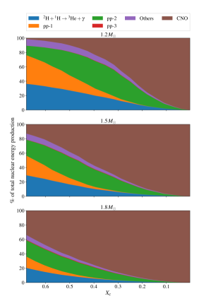
Figure 1: Share of the total energy production between the different reactions for models of $1.2$, $1.5,$ and $1.8\,M_{\odot}$ stars at solar metallicity.

Moreover, we may note that the part produced by the pp-chain is (mostly) divided between three reactions: 1) $\@element[2]{\mathrm{H}}+\@element[1]{\mathrm{H}}\rightarrow\@element[3]{\mathrm{He}}+\gamma$, which rather dominates at low temperature; 2) The pp-1 branch, $\@element[3]{\mathrm{He}}+\@element[3]{\mathrm{He}}\rightarrow\@element[4]{\mathrm{He}}+2\,\@element[1]{\mathrm{H}}$, which is the dominant way to produce $\@element[4]{\mathrm{He}}$ at low temperature; 3) The pp-2 branch, whose energy production is dominated by the contribution of the $\@element[7]{\mathrm{Li}}+\@element[1]{\mathrm{H}}\rightarrow 2\,\@element[4]{\mathrm{He}}$ reaction.

2.1.2 Timescales

To better determine the characteristics of those reactions and compare their interactions with other physical processes, we computed in the following their timescales. We defined the nuclear chemical timescale, $\tau_{i}^{\mathrm{nucl}}$, of an element $i$, similarly to Clayton (1983), by:

$$\left|\left(\frac{\partial X_{i}}{\partial t}\right)_{\mathrm{nucl}}\right|=\frac{X_{i}}{\tau_{i}^{\mathrm{nucl}}},$$ (1)

where $X_{i}$ is the mass fraction of the element. Combining this definition with the expression of $(\partial X_{i}/\partial t)_{\mathrm{nucl}}$ (e.g., Eq. 8.4 from Kippenhahn et al. 2012), we find:

$$\tau_{i}^{\mathrm{nucl}}=\frac{X_{i}\rho}{m_{i}}\left|\sum_{j}r_{j}-\sum_{k}r_{k}\right|^{-1},$$ (2)

where $\rho$ is the density, $m_{i}$ is the atomic mass of the element, $r_{j}$ is the reaction rate (number of reactions per unit of volume and time) of the reactions in which the element $i$ is a product and $r_{k}$ represents the reactions in which it is a reactant. Using MESA, we computed the values of $\tau^{\rm nucl}$ averaged over the core, for different elements, of a $1.3\,M_{\odot}$ star at solar metallicity evolved up to the moment when the central hydrogen mass fraction is $X_{c}=0.5$. Our results are listed in Table 1.

Table 1: Nuclear timescales of different elements for a $1.3\,M_{\odot}$ star at solar metallicity, evolved up to $X_{c}=0.5$

Element	Nuclear Timescale
$\@element[1]{\mathrm{H}}$	2.31 Gyr
$\@element[2]{\mathrm{H}}$	0.891 s
$\@element[3]{\mathrm{He}}$	$2.11\times 10^{5}$ yr
$\@element[4]{\mathrm{He}}$	17.6 Gyr
$\@element[7]{\mathrm{Li}}$	7.48 hours
$\@element[7]{\mathrm{Be}}$	1.60 yr
$\@element[8]{\mathrm{B}}$	156 s

2.2 Central mixing

2.2.1 Characteristics

Within the considered mass range, central mixing is attributed to convection. In stellar evolution codes, it is generally modeled in an instantaneous or diffusive way. In the first case, all elements are considered to be homogeneous in the core at every time step. This is, for example, the case of CLÉS (Scuflaire et al., 2008), ASTEC (Christensen-Dalsgaard, 2008b), and CESAM2k/CESTAM (Morel & Lebreton, 2008; Marques et al., 2013) models without microscopic diffusion. In the second case, the mixing is modeled as a very efficient diffusion process. Such implementation is found in MESA, STAROX (Roxburgh, 2008), optionally in GARSTEC (Weiss & Schlattl, 2008), and in CESAM2k or CESTAM models with microscopic diffusion. In the three first cases, the diffusion coefficient is computed with the mixing-length theory. For CESAM/CESTAM with microscopic diffusion, it is fixed at $10^{13}\,\mathrm{cm}^{2}.\mathrm{s}^{-1}$, which allows for very efficient mixing and a good numerical stability.

In this work, we use the CESTAM code without microscopic diffusion to model stars with an instantaneous mixing, along with the MESA code to model stars with a diffusive mixing. We ensured that the two codes use similar physics, and (especially) the same nuclear cross-sections. The rates are taken for both code from the NACRE compilation (Angulo et al., 1999) except for the $\@element[14]{\mathrm{N}}$ + $\@element[1]{\mathrm{H}}$ reaction, for which the rate is taken from Imbriani et al. (2005). Moreover, the two codes use the same step overshooting distance, $d_{\mathrm{ov}}$, prescription, namely, $d_{\mathrm{ov}}=\alpha_{\mathrm{ov}}\min(H_{p},R_{\mathrm{cc}})$, with $\alpha_{\mathrm{ov}}$ as a free parameter, $H_{p}$ as the pressure scale height, and $R_{\mathrm{cc}}$ as the radius of the convective core. Finally, both codes use the same solar abundances (coming from Asplund et al. (2009)), opacity tables (namely OPAL, Iglesias & Rogers 1996), and convection model, namely: the mixing length theory.

2.2.2 Timescales

In the case of an instantaneous mixing, the timescale is constant and equal to zero. In the case of a diffusive mixing, the timescale is given by:

$$\tau_{\mathrm{conv}}=\int_{0}^{R_{\mathrm{cc}}}\frac{\mathrm{d}r}{v_{\mathrm{conv}}},$$ (3)

with $R_{\rm cc}$ as the radius of the convective core and $v_{\mathrm{conv}}$ as the convective velocity determined from the mixing-length theory. Using the same model as in Sect. 2.1.1, we find $\tau_{\rm conv}=43\,\mathrm{days}$.

2.3 Impact of instantaneous mixing on central composition

When comparing the values from Table 1 with $\tau_{\rm conv}$, we can note that the nuclear timescale is lower than $\tau_{\rm conv}$ for $\@element[2]{\mathrm{H}}$, $\@element[7]{\mathrm{Li}},$ and $\@element[8]{\mathrm{B}}$. This means that they reach their mass fraction equilibrium value faster than they are mixed by convection; consequently, they are not homogeneous in the core. On the contrary, $\@element[1]{\mathrm{H}}$, $\@element[3]{\mathrm{He}}$, $\@element[4]{\mathrm{He}}$, and $\@element[7]{\mathrm{Be}}$ have a higher nuclear timescale than the convective timescale and, consequently, they are efficiently mixed and then homogeneous in the core.

We represent in Fig. 2 the mass fractions of $\@element[7]{\mathrm{Li}}$, $\@element[7]{\mathrm{Be}},$ and $\@element[2]{\mathrm{H}}$ in the core of main sequence models computed either with MESA (using a diffusive mixing) or CESTAM (using an instantaneous mixing). We also represent the composition profiles of the elements that are obtained when their nuclear equilibrium is assumed, that is, $X_{i,\mathrm{eq}}$ such that $(\partial X_{i}/\partial t)_{\mathrm{nucl}}=0$. In models with an instantaneous mixing, all the elements are by construction homogeneous in the core. This is in conflict with what we could expect from the timescale comparison: indeed, both lithium and deuterium should reach their equilibrium abundances. Therefore, we conclude that those compositions are incorrect. In models with diffusive mixing, however, we find the expected behavior: both lithium and deuterium are at the equilibrium abundance and beryllium is almost homogeneous.

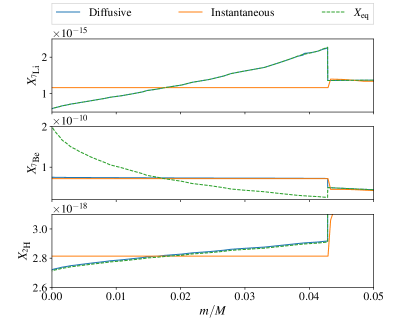
Figure 2: Abundance profiles in the core of a $1.3\,M_{\odot}$ stellar model, evolved until $X_{c}=0.5$ and computed either with MESA (central diffusive mixing) or CESTAM (central instantaneous mixing). We also represent the equilibrium abundance profiles in dotted green line.

2.4 Case when $\@element[2]{\mathrm{H}}$, $\@element[7]{\mathrm{Be}}$, $\@element[7]{\mathrm{Li}},$ and $\@element[8]{\mathrm{B}}$ are assumed to be at equilibrium

In stellar evolution codes, it is often assumed that $\@element[2]{\mathrm{H}}$, $\@element[7]{\mathrm{Be}}$, $\@element[7]{\mathrm{Li}},$ and $\@element[8]{\mathrm{B}}$ are at equilibrium at all times. This is for instance the default choice in MESA, through the parameter default_net_name = ’basic.net’. In the following we refer to those simplistic nuclear networks as “basic” networks, in opposition to the “full” networks that take into account all the nuclear timescales. Using a basic network is equivalent to assuming $\tau^{\mathrm{nucl}}=0$ for the affected elements and is justified by their short nuclear timescale compared to the typical nuclear timescale of the star (see Table 1). However, for beryllium, we note that $\tau^{\mathrm{nucl}}_{\@element[7]{\mathrm{Be}}}>\tau_{\mathrm{conv}}$ and, thus, that this element is efficiently mixed. Therefore, using a basic network yields a wrong beryllium composition profile, as we can see in Fig. 2 in which the equilibrium composition profile of this element differs from the efficiently mixed one. This faulty beryllium composition impacts in turn the lithium composition, since the latter is produced by the electronic capture of the former. Consequently, we can expect effects on the core structure that are comparable to those caused by an instantaneous mixing.

3 Impact on core structure

We observed in the previous section that using an instantaneous mixing, or a basic nuclear reaction network, has an impact on the central composition of the star. In this Section, we investigate how this change of composition impacts the structure of the convective core.

3.1 Nuclear energy production

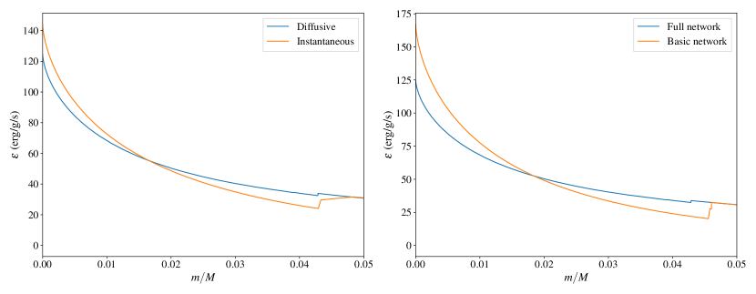
Figure 3: Rate of energy generation per unit mass. Left Panel: Models computed with either diffusive (blue) or instantaneous (orange) mixing. Right Panel: Models computed with either the full (blue) or basic (orange) network.

The nuclear energy generation rate per unit mass (noted as $\epsilon_{ij}$ for a reaction involving two reactants $i$ and $j$) is related to their mass fractions through the expression:

$$\epsilon_{ij}=\frac{1}{1+\delta_{ij}}\frac{Q_{ij}}{m_{i}m_{j}}\rho X_{i}X_{j}\langle\sigma v\rangle_{ij},$$ (4)

where $\delta_{ij}\equiv 1$ if the two reactants are identical, 0 otherwise, $Q$ the energy released per reaction, $\sigma$ is the cross-section of the reaction, and $v$ is the velocity of the particles involved in the reaction. We can conclude from this expression that the observed differences in Fig. 2 should have an impact on the nuclear energy production of the star. Moreover, this effect should not be negligible, as the reaction involving $\@element[7]{\mathrm{Li}}$ as a reactant can represent around 20% of the total nuclear energy production for stars with masses between $1.2$ and $1.8\,M_{\odot}$ (see Fig. 1). This is indeed verified in the models. Thus, models computed with different mixing prescriptions yield different $\epsilon$ profiles, as shown in the left panel of Fig. 3. Using a different nuclear network impacts $\epsilon$ comparably, as shown in the right panel of Fig. 3. We note, however, that when integrating $\epsilon$ over the core mass, we find similar core luminosities for the two models.

Additionally, we may wonder about the impact of the differences in deuterium abundance on the total energy production. Indeed, the deuterium composition profile differs between models with different mixing (see Fig. 2). Moreover, the deuterium is a reactant of a reaction ($\@element[2]{\mathrm{H}}+\@element[1]{\mathrm{H}}\rightarrow\@element[3]{\mathrm{He}}+\gamma$), which represents a significant part of the total energy production (see Fig. 1). Yet, contrary to the case of lithium, the relative differences in abundance between models with diffusive and instantaneous mixings are small (around 3%). This is due to the fact that the reactions involving deuterium are less sensitive to temperature than the ones involving lithium. Therefore, the equilibrium abundance of deuterium does not, in a relative sense, radially vary as much as the lithium abundance in the core and is less impacted by the instantaneous mixing. The impact of this difference on the total nuclear energy production is, thus, negligible.

3.2 Convective core size

For main sequence stars, which are at thermal equilibrium, the integral of $\epsilon$ over the mass inside a shell located at radius $r$ is the luminosity going through that shell, noted as $L_{r}$. We know that the radiative gradient, $\nabla_{\mathrm{rad}}=(\partial\ln T/\partial\ln p)_{\rm rad}$, is related to $L_{r}$ through the expression:

$$\nabla_{\mathrm{rad}}=\frac{3}{16\pi acG}\frac{\kappa L_{r}p}{mT^{4}},$$ (5)

where $a$ is the radiation density constant, $c$ is the velocity of light, $G$ is the gravitational constant, $\kappa$ is the Rosseland opacity, $p$ is the pressure, $T$ is the temperature, and $m$ is the mass within the sphere at the radius, $r$.

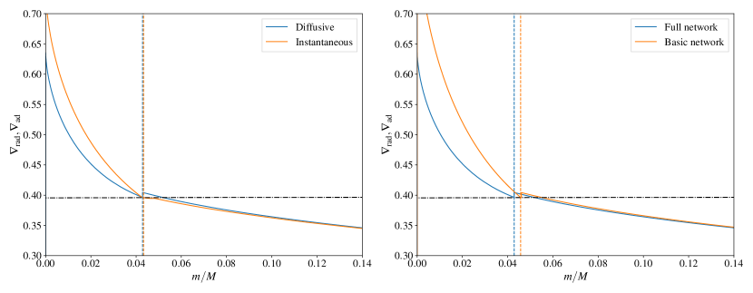
Figure 4: Radiative gradients of $1.3\,M_{\odot}$ of models, stopped at $X_{c}=0.4$. The adiabatic gradient is represented in dot-dashed black line. The vertical lines represent the core boundaries. Left Panel: Models computed with either diffusive (blue) or instantaneous (orange) mixing. Right Panel: Models computed with either the full (blue) or basic (orange) network.

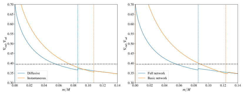
Figure 5: Same as Fig. 4, but the models are computed with $\alpha_{\mathrm{ov}}=0.15$.

Therefore, the difference in $X_{\@element[7]{\mathrm{Li}}}$ has an impact, through the $L_{r}$ term, on the radiative gradient in the core. Figs. 4 and 5 illustrate this aspect, respectively, without and with overshoot ($\alpha_{\mathrm{ov}}=0.15$). The different profiles of $\nabla_{\mathrm{rad}}$ have another striking effect on the stellar structure: for the models with overshoot, the model with an instantaneous mixing (or basic network) exhibits a bigger convective core than the model with a diffusive mixing (or full network). Such behavior is observed during the whole main sequence, as we can see in Fig. 6: the models with instantaneous mixing having a core up to 30 % more massive than the cores computed with a diffusive mixing. A similar behavior is shown in Fig. 7 for models using a basic network, which exhibit more massive cores than models using a full network.

We may note that a small region situated just outside the convective core in the MESA model is semi-convective, in the sense that it is unstable according to the Schwarzschild criterion, but stable according to the Ledoux criterion. This region has small to no impact on the stellar evolution and is quickly erased if a tiny amount of overshoot is added. Moreover, it does not exist in the CESTAM model due to the numerical scheme that smooths out the composition profile and thus lowers the opacity jump. Consequently, this semi-convective region does not impact the conclusions of this paper.

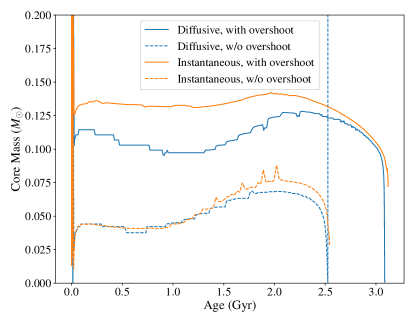
Figure 6: Core mass evolution of $1.3\,M_{\odot}$ models computed either with a diffusive (blue) or an instantaneous (orange) mixing, with (full, $\alpha_{\mathrm{ov}}=0.15$) or without (dotted) overshooting.

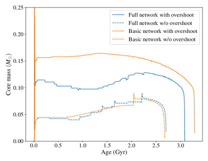
Figure 7: Core mass evolution of $1.3\,M_{\odot}$ models, using either a full (blue) or basic (orange) nuclear reaction network and computer with (full, $\alpha_{\mathrm{ov}}=0.15$) or without (dotted) overshoot.

3.3 Link with core overshooting

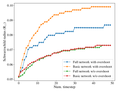
Figure 8: Evolution of the Schwarzschild radius of the convective core at the very beginning of the main-sequence, for models with a full nuclear reaction network and overshoot (blue), a basic reaction network and overshoot (orange), a full network without overshoot (green), and a basic network without overshoot (red). The 50 first time steps correspond to approximately 50 million years.

To better understand why only models with an extension of the convective core have a significantly different core size, we investigated the evolution of the convective core at the very beginning of the main sequence. To do so, we added overshooting to the core just after the initial contraction phase, once the star reached a thermal equilibrium state. Figure 8 shows the evolution of the Schwarzschild radius (i.e., the radius where $\nabla_{\mathrm{rad}}=\nabla_{\rm ad}$) for models computed with and without overshoot, and with different nuclear reactions networks, for the first 50 timesteps of the main-sequence. Similarly to models presented before, changing the nuclear reactions networks only impacts the Schwarzschild radius of models with overshoot. We noted that this process happens in a given number of time steps, rather than a given time (hence the choice of the x-axis in Fig. 8), which indicates that it is numerical rather than evolutionary. To better understand it, we introduce a toy model that mimics the behavior of the core boundary during the first time steps that follow the addition of overshooting.

In this toy model, which is illustrated in Fig. 9, we simplified the radiative gradient near the boundary of the convective core as a piecewise linear function of slopes $a^{\prime}$ in the core and $a$ in the radiative region. The adiabatic gradient is assumed to be constant. The Schwarzschild radius, where $\nabla_{\mathrm{rad}}=\nabla_{\rm ad}$, is noted as $r_{s}$ and the boundary of the fully mixed region is noted as $R_{\mathrm{cc}}$. The time step number is noted with a subscript.

At first, the core is not extended, therefore $(r_{s})_{0}=(R_{\mathrm{cc}})_{0}$. We then add overshoot over a distance $d_{\mathrm{ov}}$ such that $(R_{\mathrm{cc}})_{1}=(r_{s})_{0}+d_{\mathrm{ov}}$. At the next timestep, the Schwarzschild radius is defined by the intersection of $\nabla_{\mathrm{rad}}$ with $\nabla_{\rm ad}$ and, therefore, $(r_{s})_{1}>(r_{s})_{0}$, due to the fact that the slope of $\nabla_{\mathrm{rad}}$ is different in the core and in the radiative region. Then, overshoot is added again (we take as an approximation a constant $d_{\mathrm{ov}}$) such that $(R_{\mathrm{cc}})_{2}=(r_{s})_{1}+d_{\mathrm{ov}}$. The process is repeated at the next timestep, and $(r_{s})_{3}>(r_{s})_{2}>(r_{s})_{1}$. Eventually, this converges to a Schwarzschild radius that is significantly larger, as observed in Fig. 8.

This simple toy model allows us to derive an analytical expression for the final Schwarzschild radius, once the process is converged, that we note $(r_{s})_{\mathrm{f}}$. We find:

$$(r_{s})_{\mathrm{f}}=(r_{s})_{0}+d_{\mathrm{ov}}\left(\frac{a^{\prime}}{a}-1\right).$$ (6)

We can notice that $(r_{s})_{\mathrm{f}}$ depends on the slopes of $\nabla_{\mathrm{rad}}$ in the core and in the radiative region. Yet, the slope of $\nabla_{\mathrm{rad}}$ in the core differs between models with different mixing or nuclear reaction networks (see Fig. 4), which causes $(r_{s})_{\mathrm{f}}$ of those models to differ as well. If we note $\alpha$ and $\beta$ as the slopes of $\nabla_{\mathrm{rad}}$ in the core for two different models, assuming that they have the same radiative gradient in the radiative region (as seen in models, e.g. in Fig. 4), we find that the difference of $(r_{s})_{\mathrm{f}}$, noted as $\Delta r_{s}$, is equal to:

$$\Delta r_{s}=d_{\mathrm{ov}}\left(\frac{\alpha-\beta}{a}\right).$$ (7)

This explains the different convective core sizes for models with overshoot. Conversely, if the model has no overshoot, the different radiative gradient slopes do not impact the size of the core.

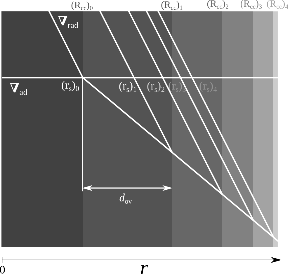
Figure 9: Schematic representation of the toy-model explained in Sect. 3.3.

3.4 Impact on the duration of the main sequence

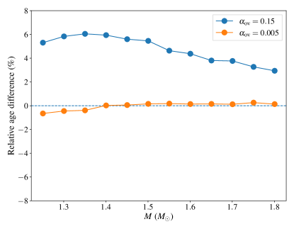
Figure 10: Relative age difference (in the sense basic - full) of models evolved until $X_{c}=0.001$, computed with $\alpha_{\mathrm{ov}}=0.15$ (blue) and $\alpha_{\mathrm{ov}}=0.005$ (orange).

It is well known that the size of the convective core impacts the duration of the main sequence. As the process described in this paper increases the size of the convective core, we investigated the change in the duration of the main sequence when using a basic nuclear reaction network rather than a full network. To do so, we computed models with different networks that evolved until the end of the main-sequence (arbitrarily defined as $X_{c}=0.001$), varying their masses. We then compared their age. Fig. 10 represents the relative age differences, in the sense of basic minus full. We observe that models computed using a basic network have a main sequence that is between 3-6% longer, depending on the mass. In order to ensure that those differences are due to the difference of core size and not the energy production, we represent the same differences computed for models with almost no overshoot, $\alpha_{\mathrm{ov}}=0.005$. Indeed, those models are supposed to have the same core size (see Fig. 6). For those models, no age difference is found, which confirms that those found for models with $\alpha_{\mathrm{ov}}=0.15$ result from the process described in this paper.

This difference in main sequence duration may impact the modeling of post-main sequence stars, inducing systematic biases in the age determination. We note that the observed differences are comparable with uncertainties inferred through seismic modeling of subgiant stars, for instance (e.g., Noll et al. 2021).

4 Impact on the seismic properties of solar-like oscillators

Stars with masses below approximately $1.5\,M_{\odot}$ are solar-like oscillators. Therefore, they exhibit numerous pressure (p) modes, which allow us to probe the internal structure of the star. Those modes are mainly sensitive to the upper structure of the star (see e.g., Aerts et al. 2010), but they are also able to probe the central region of the star. We could therefore expect that the differences in the convective core sizes observed in this work may impact the seismic observables. Thus, in this section, we describe our seismic study of solar-like pulsations using either a full nuclear reaction or a basic nuclear reaction network. We compare nuclear reaction networks rather than mixing prescriptions, because the latter would require comparisons between two different stellar evolution codes, which could potentially induce other biases.

In this section, we first study the impact of the nuclear network on the seismic observables of a grid of models. Then, we model two stars observed by Kepler to quantify the impact of using a basic reaction network on the retrieved stellar parameters.

4.1 Method

4.1.1 Characteristics of the models

All the models were computed using the MESA v10108 (Paxton et al., 2011, 2015, 2018) stellar evolution code. We used the OPAL equation of states and opacity tables (Rogers et al., 1996; Iglesias & Rogers, 1996), with a solar mixture from Asplund et al. (2009). Convective regions were computed following the mixing-length theory prescription of Cox & Giuli (1968). The mixing-length parameter $\alpha_{\mathrm{conv}}$ has been fixed to a solar-calibrated value of 1.9. Microscopic diffusion has not been taken into account. Overshooting was modeled as step extension of the convective core, with chemical mixing only: the temperature gradient is equal to the radiative gradient outside the Schwarzschild limit. The distance over which the core is extended is taken as:

$$d_{\mathrm{ov}}=\alpha_{\mathrm{ov}}\min\left(H_{p},R_{\mathrm{cc}}/\alpha_{\mathrm{conv}}\right).$$ (8)

This definition corresponds to the default definition in MESA, and differs from the one used in Sect. 3, which is the default in CESTAM. Also, we note that in the considered range of parameters, convective cores are small, which implies that $H_{p}>R_{\mathrm{cc}}/\alpha_{\mathrm{conv}}$ at the Schwarzschild radius for most of the models. The distance of overshooting is therefore generally defined as $d_{\mathrm{ov}}=\alpha_{\mathrm{ov}}R_{\mathrm{cc}}/\alpha_{\mathrm{conv}}$ in the considered mass range.

Finally, the adiabatic oscillations have been computed using ADIPLS (Christensen-Dalsgaard, 2008a). No surface effect correction has been applied, as we use seismic indicators which are almost independent of the upper layers of the star (see Section 4.1.3).

4.1.2 Characteristics of the grid

Table 2: Parameter space of the grid.

Param.	Min	Max
$M$ ($M_{\odot}$)	1.1	1.45
$[Z/X]$ (dex)	-0.2	0.35
$Y_{0}$	0.24	0.33
$\alpha_{\mathrm{ov}}$	0	0.45

We computed two grids, one using a basic network and the other one using a full reaction network. Using Sobol sequences, we computed for each grid $2^{13}=8192$ uniformly distributed tracks. The varying parameters are the stellar mass, $M$, the metallicity, $[Z/X]$, the initial helium abundance, $Y_{0}$, and the overshoot parameter. The parameter space is detailed in Table 2. For every track, 60 models have been computed during the main sequence, evenly spaced in central hydrogen abundance.

4.1.3 Definition of the seismic observables

The process studied in this article only impacts the core structure and has negligible effect on the global structure of the star. Therefore, we focused on seismic observables that are sensitive to the core structure. The small separations between the modes of degrees $l=0$ and 1 were shown to be the most sensitive to the core size (Provost et al., 2005). Moreover, Roxburgh & Vorontsov (2003) showed that the $r_{01}$ ratio is nearly insensitive to the surface layers of the star and therefore to the so-called near-surface effects. It is defined as:

$$r_{01}(n)=\frac{\nu_{n-1,0}-4\nu_{n-1,1}+6\nu_{n,0}-4\nu_{n,1}+\nu_{n+1,0}}{8\Delta\nu_{1}(n)},$$ (9)

where $\nu_{n,l}$ is the frequency of the mode of radial order $n$ and degree $l$ and $\Delta\nu_{1}(n)=\nu_{n,1}-\nu_{n-1,1}$. Finally, following Deheuvels et al. (2016), we fit to $r_{01}$ a polynomial of degree two of the type:

$$P(\nu)=a_{0}+a_{1}(\nu-\beta)+a_{2}(\nu-\gamma_{1})(\nu-\gamma_{2}),$$ (10)

and use the coefficients $a_{0}$, $a_{1}$ and $a_{2}$ as observables. Especially, $a_{0}$ and $a_{1}$ are known to be sensitive to the size of the mixed core (Silva Aguirre et al., 2011; Deheuvels et al., 2016). The addition of three more degrees of freedom, namely the coefficients $\beta$, $\gamma_{1}$, and $\gamma_{2}$, allows to ensure the independence of the $a_{k}$ coefficients. This permits the use of classical $\chi^{2}$ minimization methods (see Section 4.3.) For more details on the procedure, the reader may refer to Appendix B of Deheuvels et al. (2016). However, in this work, we used the $r_{01}$ rather than the $r_{010}$ ratio. This allowed us to avoid overfitting and greatly improved the conditioning of the covariance matrix (Roxburgh, 2018).

4.2 Impact on the seismic observables of a grid of models

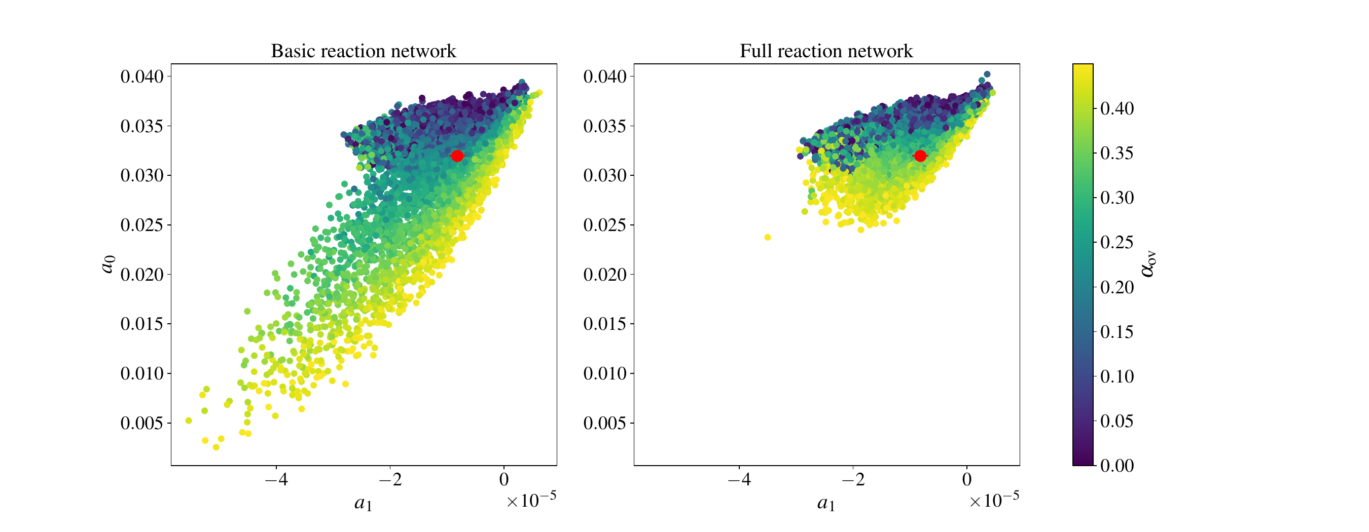
Figure 11: Representation of the models of the grid in the $(a_{1},a_{0})$ plane. Each point is colored according to the $\alpha_{\mathrm{ov}}$ value of the model. The red point represents the observational values for KIC6225718.

In this section, we adopt a “forward” approach by studying the direct impact of the change of nuclear network on the seismic observables. To do so, we computed the $a_{0}$ and $a_{1}$ coefficients for all the models of the grid. Without loss of generality, the $\beta$, $\gamma_{1}$, and $\gamma_{2}$ coefficients were chosen as those obtained from the observed frequencies of KIC6225718 (see Section 4.3.1). In order to compare models with equivalent evolutionary stage, we took models with similar mean density $\bar{\rho}$ by ensuring that they have similar large separation $\Delta\nu$, as $\Delta\nu\propto\sqrt{\bar{\rho}}$. More specifically, we ensured that all models have the same $\nu_{13,0}$ value, namely: $1510\,\mu\mathrm{Hz}$ (the observational value of KIC6225718). To do so, we linearly interpolated the $a_{k}$ coefficients along the track so that the $\nu_{13,0}$ frequency value is reproduced. The choice of reproducing a low-order frequency rather than $\Delta\nu$ allowed us to be less sensitive to surface effects, which is necessary when comparing with observations, as described in Sect. 4.3.

Figure 11 represents the $a_{0}$ and $a_{1}$ values for all the tracks of the basic network grid (left) or the full network grid (right). Each point is colored according to the $\alpha_{\mathrm{ov}}$ value of the model. For illustration, the red point indicates (as an example) the observational values for KIC6225718 and their uncertainties. We can see that modifying the nuclear reaction network has a strong impact. Indeed, for a given value of $\alpha_{\mathrm{ov}}$, models computed with a basic network have larger convective cores, which leads to lower values of both $a_{0}$ and $a_{1}$. Those differences are much greater than the represented uncertainties, meaning that they are very significant when interpreting observational data. We can also note that the models which are the most affected are those with higher values of $\alpha_{\mathrm{ov}}$. This is compatible with Eq. 7, which indicates that $\Delta r_{s}$ increases with $d_{\mathrm{ov}}$.

We note that even though the largest values of $\alpha_{\mathrm{ov}}$ computed here seem high compared to the ad-hoc value of $0.2$ often quoted in the literature, they are actually nearly equivalent. Indeed, as mentioned in Section 4.1.1, the definition of $d_{\mathrm{ov}}$ that is used here (i.e., Eq. 8) differs from the more common one, namely $d_{\mathrm{ov}}=\alpha_{\mathrm{ov}}\min\left(H_{p},R_{\mathrm{cc}}\right)$. Therefore, a ratio of up to $\alpha_{\mathrm{conv}}$ (1.9 in our case) is found between equivalent overshoot parameter.

4.3 Impact on seismic modeling

4.3.1 Observational data and modeling method

We seismically modeled two stars observed by Kepler, namely, KIC6225718 and KIC12258514, to quantify the impact of using a basic network on the inferred stellar parameters. We used the frequencies of Lund et al. (2017) to compute the ratios and the $a_{k}$ coefficients. To find their uncertainties, we performed Monte Carlo simulations with 10000 iterations. Finally, we added two spectroscopic observables: the surface metallicity, $[\mathrm{Fe}/\mathrm{H}]_{\mathrm{spec}}$, and the effective temperature. $T_{\mathrm{eff}}$. Both are taken from Bruntt et al. (2012).

We found the best models by minimizing the following quantity:

$$\chi^{2}=\sum_{i=1}^{5}\frac{\left(x_{i}^{\mathrm{mod}}-x_{i}^{\mathrm{obs}}\right)^{2}}{\sigma_{i}^{2}},$$ (11)

where $x_{i}^{\mathrm{obs}}$ are the observables (namely the $a_{0}$, $a_{1}$ and $a_{2}$ coefficients, $T_{\mathrm{eff}}$ and $[Z/X]_{\mathrm{spec}}$), $x_{i}^{\mathrm{mod}}$ the equivalent values computed with the stellar models, and $\sigma_{i}$ the observational uncertainties. We computed the uncertainties on the model parameters by dividing by 6 the range of parameters of models whose $\chi^{2}$ is inferior to $\chi^{2}_{\min}+9$.

4.3.2 Results

Table 3: Parameters of the best model for KIC6225718 and KIC12258514

Network	$M$ ($M_{\odot}$)	$R$ ($R_{\odot}$)	Age (Gyr)	$[Z/X]_{\mathrm{init}}$ (dex)	$Y_{0}$	$\alpha_{\mathrm{ov}}$	$X_{c}$
KIC6225718
Basic	$1.265\pm 0.030$	$1.268\pm 0.011$	$1.818\pm 0.316$	$0.076\pm 0.064$	$0.248\pm 0.012$	$0.202\pm 0.044$	$0.512\pm 0.054$
Full	$1.287\pm 0.022$	$1.276\pm 0.009$	$1.790\pm 0.317$	$0.093\pm 0.055$	$0.240\pm 0.011$	$0.282\pm 0.052$	$0.522\pm 0.049$
KIC12258514
Basic	$1.316\pm 0.017$	$1.627\pm 0.009$	$4.078\pm 0.156$	$0.150\pm 0.045$	$0.251\pm 0.009$	$0.124\pm 0.015$	$0.060\pm 0.012$
Full	$1.314\pm 0.027$	$1.626\pm 0.012$	$4.185\pm 0.256$	$0.121\pm 0.051$	$0.243\pm 0.013$	$0.154\pm 0.028$	$0.058\pm 0.012$

The parameters of the best models for the two stars, using either a basic or a full nuclear reaction network, are summarized in Table 3. In both cases, we find that the overshoot parameters of the best models are significantly different between the two models, with differences approximately equal to $1.5\,\sigma$. However, all the other stellar parameters are identical within the uncertainties. We can therefore conclude that (at least for those two stars) modifying the overshoot parameter alone is enough to compensate the core size differences caused by the change of nuclear reactions network.

We note that in this study, we left $\alpha_{\mathrm{ov}}$ as a free parameter. However, if it is fixed, either through a mass-dependent prescription or an ad-hoc value, it may induce biases on the other parameters of the star.

5 Discussions and conclusions

In this paper, we show how some simplistic assumptions on convection mixing and nuclear reactions that are commonly made in stellar evolution codes may impact the size of convective cores of low-mass stars. First, assuming an instantaneous mixing in the core leads to erroneous central composition profiles. In particular, lithium has a nuclear timescale (of the order of an hour) that is much shorter than the convective timescale (of the order of a month): it is therefore not homogeneous in the core. The resulting difference of composition between models with a diffusive and an instantaneous mixing impacts the nuclear production of the pp-2 chain, which can represent up to 20% of the total nuclear energy production for $\sim 1.5\,M_{\odot}$ stars. Thus, the profile of the radiative gradient in the core is affected, leading to differences in the sizes of the convective cores of models with overshoot. Those discrepancies, which depend mainly on the evolutionary stage, mass, and overshoot parameter of the model, can represent up to 30% of the core mass for $\alpha_{\mathrm{ov}}=0.15$.

Moreover, we observed that using a “basic” nuclear reaction network, which considers beryllium at nuclear equilibrium, has a similar effect. Indeed, the comparison between the nuclear and convective timescales tells us that beryllium is actually efficiently mixed while lithium is not. This affects the lithium composition, which eventually results in core size differences that are similar to those observed when assuming an instantaneous mixing. Notably, those core size differences affect the duration of the main-sequence, models with basic networks having a longer main sequence by around 6% for $\alpha_{\mathrm{ov}}=0.15$.

We then studied the impact of those core size discrepancies on the seismic modeling of solar-like oscillators. To do so, we modeled two stars observed by Kepler using ratios of their oscillation frequencies, as those are the most sensitive to the central structure. We computed models using either a full nuclear reaction network or a basic one. We found that for the two stars, the overshoot parameter of the best model with a basic network is significantly smaller than the overshoot parameter of the best model with a full network. Apart from that, the other parameters are identical. We conclude that modifying the overshoot parameter is sufficient to compensate the core size difference caused by using an overly simplified nuclear reaction network. However, if this parameter is fixed while modeling the star, those core sizes differences may induce biases on other parameters. From this result we conclude that it is necessary, for a proper modeling of low-mass stars with a convective core, to both consider a diffusive convective mixing and a full nuclear reaction network. This is particularly important in the framework of the preparation of future missions such as Plato (Rauer et al., 2014), where the proper determination of the age of main sequence and subgiant stars is crucial.

In this study, we focus on models with step overshooting. However, we note the interesting result of Zhang et al. (2022), who pointed out another consequence of the comparison between $\tau_{\mathrm{conv}}$ and $\tau_{\mathrm{nucl}}$ for models with exponential overshoot. Indeed, within an exponential overshoot region, the diffusion mixing coefficient radially varies, and so does $\tau_{\rm conv}$. Therefore, the radius where $\tau_{\rm conv}$ becomes higher than $\tau_{\rm nucl}$ (i.e., the radius where the element is not efficiently mixed) is different for each element. Consequently, the distance over which the elements are mixed differ depending on their nuclear timescale, as can be seen in the compositional profiles on Fig. A1 of that paper.

Moreover, we only studied the impact on the modeling of solar-like oscillators. However, there are other types of oscillators found within this mass range. In particular, $\gamma$ Doradus are stars exhibiting gravity modes during the main sequence, with masses between approximately $1.5$ and $1.8\,M_{\odot}$ (e.g., Aerts et al. 2010). Their modes are particularly sensitive to the core properties (Miglio et al., 2008) and have already been used to constrain the overshoot parameter (Mombarg et al., 2019, 2021). Therefore, the recommendations of using a full nuclear network and a diffusive mixing should also be followed when studying this type of oscillator.