DES Y3 + KiDS-1000: Consistent Cosmology combining cosmic shear surveys

Abstract

We present a joint cosmic shear analysis of the Dark Energy Survey (DES Y3) and the Kilo-Degree Survey (KiDS-1000) in a collaborative effort between the two survey teams. We find consistent cosmological parameter constraints between DES Y3 and KiDS-1000 which, when combined in a joint-survey analysis, constrain the parameter $S_{8}=\sigma_{8}\sqrt{\Omega_{\rm m}/0.3}$ with a mean value of $0.790^{+0.018}_{-0.014}$. The mean marginal is lower than the maximum a posteriori estimate, $S_{8}=0.801$, owing to skewness in the marginal distribution and projection effects in the multi-dimensional parameter space. Our results are consistent with $S_{8}$ constraints from observations of the cosmic microwave background by Planck, with agreement at the $1.7\sigma$ level. We use a Hybrid analysis pipeline, defined from a mock survey study quantifying the impact of the different analysis choices originally adopted by each survey team. We review intrinsic alignment models, baryon feedback mitigation strategies, priors, samplers and models of the non-linear matter power spectrum.

1 Introduction

A cosmic shear analysis exploits the weak gravitational lensing of background galaxy images by foreground large-scale structures in order to probe the growth of structures and the expansion of the Universe. Since the first detection (Bacon et al., 2000; Kaiser et al., 2000; Van Waerbeke et al., 2000; Wittman et al., 2000) significant developments in instrumentation, data, theory, simulation and statistical analysis have led to an established and robust cosmological probe. Cosmic shear is one of the primary science drivers for the next generation of cosmological surveys imaged with Euclid, the Nancy Grace Roman Space Telescope and the Vera C. Rubin Observatory. These surveys are designed to attain sub-percent level precision on joint measurements of the dark energy equation of state parameter, $w_{0}$, and the scale factor evolution parameter, $w_{\rm a}$. Their goal is to understand the mechanism that drives cosmic acceleration. Large-scale pathfinders include the Deep Lens Survey (DLS, Wittman et al., 2002; Jee et al., 2016), the Canada France Hawaii Telescope Lensing Survey (CFHTLenS, Heymans et al., 2012; Joudaki et al., 2017), the Dark Energy Survey (DES, DES Collaboration et al. 2018; Sevilla-Noarbe et al. 2021; Amon et al. 2022; Secco, Samuroff et al. 2022), the Hyper Suprime Camera Survey (HSC, Aihara et al., 2018; Dalal et al., 2023; Li et al., 2023a) and the Kilo Degree Survey (KiDS, Kuijken et al., 2015, 2019; Asgari et al., 2021). All have set tight and consistent constraints on the parameter $S_{8}=\sigma_{8}\sqrt{\Omega_{\mathrm{m}}/0.3}$, which accounts for the inherent cosmic shear degeneracy between $\Omega_{\mathrm{m}}$, the matter density parameter, and $\sigma_{8}$, the linear-theory standard deviation of matter density fluctuations in spheres of radius $8\,h^{-1}\mathrm{Mpc}$. These constraints all show a preference for $S_{8}$ to be lower than the value derived from observations of the Cosmic Microwave Background when adopting the flat-$\Lambda$CDM model (CMB; Planck Collaboration, 2020). Any significant offset between direct measurements of $S_{8}$ and the CMB-informed $\Lambda$CDM prediction would, in principle, indicate issues with the $\Lambda$CDM model. The community has not reached a consensus on whether the ‘tension’ seen between these early and late Universe observations arises from sampling variance, systematic errors in the theoretical modelling and/or data analysis, or whether the existing results are already an indication of beyond-$\Lambda$CDM physics.

The weak lensing community has a long history of collaborative initiatives to improve the robustness of cosmic shear cosmology with shear and redshift measurement challenges analysing image simulations and mock catalogues (Heymans et al., 2006a; Hildebrandt et al., 2010; Kitching et al., 2012; Mandelbaum et al., 2015; Euclid Collaboration: Desprez et al., 2020; Schmidt et al., 2020). The strong track record in releasing all relevant data products has also allowed for examination and verification by independent groups (MacCrann et al. 2015; Efstathiou & Lemos 2018; Troxel et al. 2018; Asgari et al. 2019; Asgari, Tröster et al. 2020; Joudaki et al. 2020; Chang et al. 2019; García-García et al. 2021; Amon & Efstathiou 2022; Longley et al. 2023). Comparison studies find consistent weak lensing measurements between different surveys, as quantified through measurements of the projected surface mass density around luminous red galaxies (Amon et al.,, 2018; Leauthaud, Amon et al., 2022; Amon, Robertson et al., 2023). Unified analyses of cosmic shear surveys also find consistency between the surveys tested, but highlight the impact of different analysis choices on the recovered cosmological parameter constraints (Benjamin et al. 2007; Chang et al. 2019; Asgari, Tröster et al. 2020; Joudaki et al. 2020). Most recently, Longley et al. (2023) combined the first year data from DES and HSC with the fourth data release from KiDS, reporting the tightest Stage-III cosmic shear constraints to date. The 1.6-1.9% constraints on $S_{8}$ range from $S_{8}=0.777^{+0.016}_{-0.017}$ to $S_{8}=0.791^{+0.013}_{-0.013}$, depending on the different modelling approaches and methods used to account for the cross-survey covariance between the overlapping KiDS and HSC surveys.

This paper presents a joint collaboration analysis of the latest data releases from the Dark Energy Survey (hereafter DES Y3), and the Kilo-Degree Survey (hereafter KiDS-1000). Table 1 summarises the survey specifications for these two complementary data sets. The DES footprint spanning a factor of five times the area of the KiDS footprint, can be contrasted with KiDS utilising three times as many filters as DES in the wide field cosmic shear measurement, with matched-depth photometry in both the optical and near infrared. In the DES Deep Field calibration analysis, DES extend both the depth and wavelength range of the survey into the near infrared (Hartley, Choi et al., 2021). To advance photometric redshift calibration, both surveys incorporate significant imaging of calibration fields that have been targeted by a range of different deep spectroscopic redshift campaigns (Hildebrandt, van den Busch, Wright et al., 2021; Myles, Alarcon et al., 2021). Using self-organising maps (SOM), both teams mitigate incompleteness in these spectroscopic training samples (Buchs et al. 2019; Wright et al. 2020a; Myles, Alarcon et al. 2021), incorporating near-infrared information (Wright et al. 2019; Hartley, Choi et al. 2021; Everett et al. 2022), with validation using cross-correlation clustering measurements (van den Busch et al. 2020; Hildebrandt, van den Busch, Wright et al. 2021; Gatti, Giannini et al. 2022b). DES and KiDS both adopt blinding procedures to avoid the inclusion of confirmation bias in their findings (Kuijken et al., 2015; Muir et al., 2020). The cosmic shear constraints from the two surveys are consistent, with similar prescriptions chosen to derive analytical covariance matrices (Schneider et al., 2002; Joachimi et al., 2021; Friedrich et al., 2021). Asgari et al. (2021) present the KiDS-1000 cosmic shear analysis finding $S_{8}=0.759_{-0.021}^{+0.024}$. Amon et al. (2022); Secco, Samuroff et al. (2022) present the DES Y3 joint cosmic shear and shear ratio analysis finding $S_{8}=0.772^{+0.018}_{-0.017}$ in their $\Lambda$CDM-optimised analysis.

Whilst there are many similarities between the DES and KiDS data processing techniques, catalogue production and calibration methods, it is worth noting that the two teams take rather different approaches to the shear measurement (Miller et al., 2013; Huff & Mandelbaum, 2017; Sheldon & Huff, 2017). This has been motivated in part by the different tiling strategies and PSF properties of each survey. The DES analysis operates on astrometrically sheared and stacked images with the KiDS analysis operating on individual unsheared exposures using analytic astrometric corrections. These core differences in data handling make it highly non-trivial to conduct a KiDS-like shear measurement of DES and vice versa. Many in the lensing community argue that the significant resources required to make a pixel-level comparison of shear measurement methods using real data would be unwarranted, given the significant investment already made in the production of realistic image simulations (Kannawadi et al., 2019; MacCrann et al., 2022; Li et al., 2023c). This argument is strengthened by the finding that the simulation-informed calibration correction is fairly insensitive to modifications of the simulation’s input parameters, well within the uncertainty adopted by each team (see for example appendix C of Li et al., 2023b). We are therefore confident in the compatibility and robustness of the DES and KiDS shear catalogues for this joint-survey analysis.

In this analysis we quantify how the cosmological parameter constraints for DES and KiDS are impacted by differences in the model and analysis framework chosen by each survey. Table 2 highlights these methodological differences, which, in each case, have been chosen based on well-reasoned and sound scientific arguments detailed in Joachimi et al. (2021) and Krause et al. (2021). We present constraints from a Hybrid pipeline where we adopt a unified set of choices designed to provide the most robust joint-survey analysis. We adopt the findings of each team for their overall covariance matrix and their quantification of redshift and shear calibration uncertainty, following any survey-specific data-related systematic limitations and mitigation strategies.

This paper is organised as follows. In Section 2 we review the differences in methodology and the analysis framework between the two survey teams, along with our choices and rationale behind the Hybrid pipeline. Cosmological parameter constraints are presented in Section 3 with our conclusions presented in Section 4. Detailed information about the analysis can be found in the appendices. Appendix A presents the DES data vector used in the joint-survey analysis, re-measured from the DES Y3 catalogues with the overlapping region of the KiDS footprint excised to mitigate cross-survey covariance. Appendix B defines the required scale cuts for the DES and KiDS data vectors when using the DES baryon feedback mitigation strategy. Appendix C presents a study of the impact of the different analysis choices within a controlled mock data environment. We compare constraints when the astrophysical systematics are matched to each survey’s framework and consider potential systematic biases in a joint-survey analysis when the underlying astrophysical systematic models are no-longer matched to the models adopted by each survey. Appendix D compares the differences between the recovered cosmological constraints from a range of samplers and in Appendix E we verify the accuracy of our Hybrid pipeline using mock data based on the EuclidEmulatorv2 (Euclid Collaboration: Knabenhans et al., 2021). Appendix F quantifies the probability of finding an offset in $S_{8}$ when comparing noisy cosmic shear constraints with and without scale cuts. Finally in Appendix G we present additional tables and figures to complement the primary analysis in Section 3.

	DES Y3	KiDS-1000	HSC Year 3
Cosmic shear catalogue:
Area ${\rm[deg^{2}]}$	4143	777	416
Wavebands	riz (Wide) +	${\it ugriZYJHK_{s}}$	grizy
	${\it grizJHK_{s}}$ (Deep)
$n_{\rm eff}$	5.59	6.22	14.96
$z_{\rm median}$	0.63	0.67	0.80
2-pt statistic	$\xi_{\pm}(\theta)$	COSEBIs	$\xi_{\pm}(\theta){C_{\epsilon\epsilon}}(\ell)$
	DES Y3	KiDS-1000
Data calibration uncertainty:
Shear	$m_{1}:{\cal G}(-0.006;0.009)$	$\mbox{\boldmath$\Delta m$}:{\cal N}(\mbox{\boldmath$\mu$}_{m};\mbox{\boldmath$C$}_{m})$
	$m_{2}:{\cal G}(-0.020;0.008)$	$\mu_{m}^{1}=-0.009\,\,\,\,\sigma_{m}^{1}=0.019$
	$m_{3}:{\cal G}(-0.024;0.008)$	$\mu_{m}^{2}=-0.011\,\,\,\,\sigma_{m}^{2}=0.020$
	$m_{4}:{\cal G}(-0.037;0.008)$	$\mu_{m}^{3}=-0.015\,\,\,\,\sigma_{m}^{3}=0.017$
		$\mu_{m}^{4}=\,\,\,\,0.002\,\,\,\,\sigma_{m}^{4}=0.012$
		$\mu_{m}^{5}=\,\,\,\,0.007\,\,\,\,\sigma_{m}^{5}=0.010$
Redshift	$\Delta z_{1}:{\cal G}(0;0.018)$	$\mbox{\boldmath$\Delta z$}:{\cal N}(\mbox{\boldmath$\mu$}_{z};\mbox{\boldmath$C$}_{z})$
	$\Delta z_{2}:{\cal G}(0;0.015)$	$\mu_{z}^{1}=\,\,\,\,0.000\,\,\,\,\sigma_{z}^{1}=0.011$
	$\Delta z_{3}:{\cal G}(0;0.011)$	$\mu_{z}^{2}=\,\,\,\,0.002\,\,\,\,\sigma_{z}^{2}=0.011$
	$\Delta z_{4}:{\cal G}(0;0.017)$	$\mu_{z}^{3}=\,\,\,\,0.013\,\,\,\,\sigma_{z}^{3}=0.012$
		$\mu_{z}^{4}=\,\,\,\,0.011\,\,\,\,\sigma_{z}^{4}=0.009$
		$\mu_{z}^{5}=-0.006\,\,\,\,\sigma_{z}^{5}=0.010$

Table 1: The properties of the DES Y3, KiDS-1000 and HSC Year 3 cosmic shear catalogue (upper section). The area listed corresponds to the total area of the survey footprint after masking. The wavebands utilised for the analysis are listed, with DES analysing the riz filters in the Wide Survey area, using extra depth and wavelength coverage in the Deep Fields for calibration (Hartley, Choi et al., 2021). The effective number density of sources, $n_{\rm eff}$, is given in units of galaxies per square arcmin (Heymans et al., 2012). For DES Y3 and KiDS-1000 we list the observational systematic nuisance parameters used in this analysis (lower section). Uncertainty on the shear, $m_{i}$, and redshift calibration corrections, $\Delta z_{i}=\langle n_{i}^{\rm estimate}(z)\rangle-\langle n_{i}^{\rm true}(z)\rangle$, per tomographic bin $i$, are modelled as uncorrelated between the four DES tomographic bins. DES uses independent Gaussian priors ${\cal G}(\mu;\sigma)$, with mean $\mu$ and standard deviation $\sigma$. Data calibration uncertainty is modelled as correlated between the five KiDS tomographic bins, using a five dimensional multivariate Gaussian prior ${\cal N}(\mbox{\boldmath$\mu$};\mbox{\boldmath$C$})$ with mean, $\mu$, and covariance, $C$. The amplitude of the diagonal of the covariance is listed as $\sigma^{i}=\sqrt{C^{ii}}$.

2 Cosmic Shear Analysis

In this paper, the term ‘cosmic shear’ refers to the two-point statistical analysis of the observed correlations between galaxy ellipticities, $\epsilon^{\rm obs}$, which are related to the weak gravitational lensing shear $\gamma$ as

$$\epsilon^{\rm obs}=(1+m)\left[\epsilon^{\rm int}+\eta+\alpha\epsilon^{*}+\beta\delta\epsilon^{*}+c+\gamma\right],$$ (1)

where $\epsilon^{\rm int}$ is the intrinsic galaxy ellipticity, $\eta$ is the random noise on the measurement, $\epsilon^{*}$ is the model ellipticity of the image point spread function (PSF), $\delta\epsilon^{*}$ is the error on the PSF ellipticity model, $c$ is an additive bias that is uncorrelated with the PSF and $\alpha$, $\beta$ and $m$ are scalars that may vary for different galaxy samples (Heymans et al., 2006a; Paulin-Henriksson et al., 2008; Jarvis et al., 2016).

For a perfect shape measurement method, $m=0$, $c=0$, $\alpha=0$ and $\delta\epsilon^{*}=0$, for all galaxies. Both DES and KiDS use image simulations to quantify the amplitude and uncertainty of the multiplicative calibration correction $m$ (Kannawadi et al., 2019; MacCrann et al., 2022). They also both quantify the additive calibration correction terms empirically with a significant detection of mean ellipticity in both DES, $\langle\epsilon^{\rm obs}_{1}\rangle=(3\pm 1)\times 10^{-4}$ (Gatti et al., 2021), and KiDS, $\langle\epsilon^{\rm obs}_{2}\rangle=(6\pm 1)\times 10^{-4}$ (Giblin et al., 2021). This additive bias is corrected by subtracting the average ellipticity, per tomographic bin, to ensure that the mean shear is zero by definition. Both teams then verify that the mild levels of PSF contamination detected are sufficiently low so as not to bias cosmological parameter constraints (Giblin et al. 2021; Jarvis et al. 2021; Gatti et al. 2021; Amon et al. 2022). As such, we only correct for the multiplicative and additive shear calibration terms, $m$ and $c$, in Equation 1. The resulting corrected shear angular power spectrum ${C_{\epsilon\epsilon}}^{\rm corr}(\ell)$ then contains signal from both gravitational lensing (G) and the intrinsic (I) alignment of galaxies,

$${C_{\epsilon\epsilon}}^{\rm corr}(\ell)=C_{\rm GG}(\ell)+C_{\rm GI}(\ell)+C_{\rm II}(\ell)\;.$$ (2)

In this section, we summarise the approach taken in the DES (Amon et al. 2022; Secco, Samuroff et al. 2022) and KiDS (Asgari et al., 2021) cosmic shear analyses to model each component in equation 2 and constrain cosmological parameters. The differing methodology has been rigorously tested by each collaboration to the accuracy required by each survey (Joachimi et al., 2021; Krause et al., 2021). Given the additional constraining power of a joint-survey analysis, we review each survey’s analysis choices in Appendices C and E utilising information from recent N-body and hydrodynamical simulations (Euclid Collaboration: Knabenhans et al., 2021; van Daalen et al., 2020). Motivated by our findings, we define a set of unified analysis choices which we adopt in our fiducial Hybrid analysis in Section 3. Here our aim has been to design the most robust pipeline possible for a joint-survey analysis. In the case of some of our Hybrid analysis choices, the decisions are either subjective by nature (for example the choice of priors and parameters), or else there is simply not enough information at present to make an informed decision (for example the complexity of the IA model). For these elements, we have made decisions based on input from the two collaborations, adopting the best available options suited for a joint-survey analysis at this point in time.

	DES Y3	KiDS-1000	Hybrid
Cosmological parameter priors:
Amplitude	$A_{\mathrm{s}}:\left[0.5,\,5.0\right]$	$S_{8}:\left[0.1,1.3\right]$	$S_{8}:\left[0.1,1.3\right]$
Hubble constant	$h:\left[0.55,0.91\right]$	$h:\left[0.64,0.82\right]$	$h:\left[0.64,0.82\right]$
Matter density	$\Omega_{\mathrm{m}}:\left[0.1,0.9\right]$	$\omega_{\rm c}:\left[0.051,0.255\right]$	$\omega_{\rm c}:\left[0.051,0.255\right]$
Baryon density	$\Omega_{\mathrm{b}}:\left[0.03,0.07\right]$	$\omega_{\mathrm{b}}:\left[0.019,0.026\right]$	$\omega_{\mathrm{b}}:\left[0.019,0.026\right]$
Spectral index	$n_{\mathrm{s}}:\left[0.87,\,1.07\right]$	$n_{\mathrm{s}}:\left[0.84,\,1.1\right]$	$n_{\mathrm{s}}:\left[0.84,\,1.1\right]$
Neutrinos	$1000\,\Omega_{\nu}h^{2}:\left[0.6,6.44\right]$	$\Sigma m_{\nu}=0.06{\rm eV}$	$\Sigma m_{\nu}=\left[0.055,0.6\right]{\rm eV}$
Astrophysical systematic models and priors:
Intrinsic Alignments	TATT: $b_{\rm TA}:\left[0,2\right]$; $a_{1},a_{2},\eta_{1},\eta_{2}:\left[-5,5\right]$	NLA: $A_{\rm IA}:\left[-6,6\right]$	NLA-z: $A_{\rm IA},\eta_{\rm IA}:\left[-5,5\right]$
Non-linear Model	Halofit	HMCode2016	HMCode2020
Baryon Feedback	Scale cuts	$A_{\rm bary}:\left[2,3.13\right]$	Scale cuts & $\log_{10}(T_{\rm AGN}/{\rm K}):\left[7.3,8.0\right]$
Neutrino Model	Bird et al. (2012)	HMCode2016	HMCode2020
Sampling Algorithm:
	PolyChord	MultiNest	PolyChord

Table 2: Comparison of the modelling choices in the DES-like, KiDS-like and Hybrid cosmic shear analyses: cosmological parameters, astrophysical systematic models and the chosen sampling algorithm. The values in square brackets are the limits of the adopted top-hat priors. The listed cosmological parameters are: the amplitude of the primordial power spectrum of scalar density fluctuations, $A_{\rm s}$; the Hubble constant, $h=H_{0}/(100\,{\rm km}\,{\rm s}^{-1}\,{\rm Mpc}^{-1})$; the matter density, $\Omega_{\rm m}$; the baryon density, $\Omega_{\rm b}$; the scalar spectral index, $n_{\rm s}$; the neutrino mass density parameter, $\Omega_{\nu}$; $S_{8}=\sigma_{8}\sqrt{\Omega_{\mathrm{m}}/0.3}$, where $\sigma_{8}$ is the linear-theory standard deviation of matter density fluctuations in spheres of radius $8\,h^{-1}\mathrm{Mpc}$; $\omega_{\rm c}=\Omega_{\rm c}h^{2}$, where $\Omega_{\rm c}$ is the cold dark matter density; $\omega_{\rm b}=\Omega_{\rm b}h^{2}$; and the sum of the neutrino masses, $\Sigma m_{\nu}$.

2.1 Non-linear matter power spectrum

The DES and KiDS teams both choose to relate the convergence power spectrum, $C_{\rm GG}(\ell)$, to the non-linear matter power spectrum $P_{\rm\delta}(k,z)$, using a modified flat sky Limber approximation (LoVerde & Afshordi, 2008; Kilbinger et al., 2017)

$$C_{\rm GG}^{(ij)}(\ell)=\int_{0}^{\chi_{\mathrm{hor}}}{\rm d}\chi\>\frac{W^{(i)}(\chi)W^{(j)}(\chi)}{f_{\rm K}^{2}(\chi)}P_{\rm\delta}\left(\frac{\ell+1/2}{f_{\mathrm{K}}(\chi)},\chi\right)\;.$$ (3)

Here $f_{\rm K}(\chi)$ is the comoving angular diameter distance which simplifies to $\chi$, the radial comoving distance, for a spatially flat Universe, and the integral is taken to the horizon, $\chi_{\rm hor}$. The kernel, $W$, depends on the redshift distribution of the correlated tomographic populations, $i$ or $j$, with the mathematical form found in equations 6.19 and 6.22 of Bartelmann & Schneider (2001).

Each team calculates the linear matter power spectrum using CAMB (Lewis et al., 2000), and uses a halo model approach, calibrated with numerical simulations, to determine the non-linear correction. The details of this correction, however, differ. The DES team adopts the Smith et al. (2003) Halofit fitting formula, re-calibrated by Takahashi et al. (2012), where the impact of a non-zero neutrino mass is modelled using the CAMB-version of the Bird et al. (2012) fitting formula. The KiDS team adopts the HMCode2016 model from Mead et al. (2015), with the appropriate extensions for non-zero neutrino mass (Mead et al., 2016). In our Hybrid analysis we adopt HMCode2020, an updated version of this model, which delivers improved accuracy at the level of $<2.5\%$ to $k<10\,h\,\mathrm{Mpc}^{-1}$ (see Mead et al., 2021, and Appendix E.1).

2.2 Intrinsic galaxy alignments

The intrinsic alignment (IA) of galaxies with their local environment can mimic weak lensing and therefore this phenomenon is included as an astrophysical systematic uncertainty in all cosmic shear analyses, with a range of different analytical models proposed to mitigate this effect (see Troxel & Ishak, 2015; Joachimi et al., 2015; Kiessling et al., 2015, and references therein).

The KiDS team adopts the non-linear linear-alignment model (NLA) which describes the linear tidal alignment of galaxies with the density field (Hirata & Seljak, 2004). This model also includes an ad hoc non-linear correction to the linear matter power spectrum (Bridle & King, 2007), as motivated by intrinsic alignment measurements in numerical simulations and the Sloan Digital Sky Survey (Heymans et al., 2006b; Hirata et al., 2007). The fiducial KiDS analysis allows for only one free nuisance parameter, $A_{\rm IA}$, modulating the amplitude of the intrinsic alignment model (see equations 3-5 in Bridle & King 2007 for the NLA intrinsic alignment power spectra, $C_{\rm GI}$ and $C_{\rm II}$). The NLA model can also include flexibility where the amplitude of the IA signal depends on the average luminosity of each tomographic sample (Joachimi et al., 2011). More commonly used, however, is an NLA model amplitude that evolves with redshift, using a power-law with $[(1+z)/(1+z_{\rm pivot})]^{\eta_{\rm IA}}$, hereafter referred to as the NLA-z model.

The DES team adopts the Tidal Alignment and Tidal Torquing model (TATT, Blazek et al., 2019), which extends the linear alignment model with the inclusion of a tidal torquing alignment mechanism. The fiducial DES analysis allows for five free nuisance parameters: a tidal alignment amplitude, $a_{1}$, with redshift evolution, $\eta_{1}$; a tidal torquing amplitude, $a_{2}$, with redshift evolution, $\eta_{2}$; a linear bias amplitude, $b_{\rm TA}$ (see equations 37-39 in Blazek et al., 2019, for the TATT intrinsic alignment power spectra, $C_{\rm GI}$ and $C_{\rm II}$, highlighting the expectation of a non-zero B-mode from the ‘II’ term). In the limit $a_{2}$, $\eta_{2}$, $b_{\rm TA}\rightarrow 0$, the TATT model reduces to the NLA-z model with $a_{1}=A_{\rm IA}$ and $\eta_{1}=\eta_{\rm IA}$.

Both the NLA and TATT models are found to provide a sufficiently good fit to numerical simulations (Secco, Samuroff et al. 2022; Hoffmann et al. 2022). Currently there is no observational evidence to support the use of one model over the other in two-point cosmic shear analyses. For our Hybrid analysis we choose to adopt the NLA-z model. In terms of complexity, this is between the original choices of the two survey teams. In our fiducial Hybrid analysis we adopt independent IA parameters for each survey to reflect the different survey depths, selection functions, shape measurement methods and photometric redshift errors which can be absorbed by the IA model (for further discussion, see Appendix C.2).

2.3 Baryon feedback

Studies of hydrodynamical simulations find significant differences in the small-scale, $k>0.1h{\rm Mpc}^{-1}$, total matter distribution relative to dark matter-only simulations, as a result of baryon cooling, star formation and active galactic nuclei (AGN) feedback (see Chisari et al., 2019, and references therein). Theoretical models of the non-linear matter power spectrum, $P_{\delta}(k,z)$, that have been calibrated using dark matter-only simulations are therefore inaccurate at high-$k$ (White, 2004; Semboloni et al., 2011). There is, however, a large degree of uncertainty on the scale, amplitude and redshift dependence of baryon feedback.

To account for this uncertainty the KiDS team adopts the HMCode non-linear matter power spectrum $P_{\rm\delta}(k,z)$ model, which incorporates uncertainty from baryon feedback through a single free parameter. This parameter scales the halo concentration and the stellar and gas content, leading to a modification in the overall amplitude and shape of the ‘one-halo’ term in the halo model. Asgari et al. (2021) utilise the Mead et al. (2016) version of HMCode, calibrated with the OWLS hydrodynamical simulations (van Daalen et al., 2011). Tröster et al. (2021) present a KiDS-1000 cosmic shear band power spectrum re-analysis using HMCode2020, calibrated with the updated BAHAMAS hydrodynamical simulations (McCarthy et al., 2017; van Daalen et al., 2020).

DES take a different approach to mitigating baryon feedback uncertainty in their analysis, eliminating data on scales which are expected to be impacted significantly. Taking the ‘worst-case scenario’ for the extent of the impact as the AGN model from the suite of OWLS hydrodynamical simulations (van Daalen et al., 2011), Krause et al. (2021) contaminate a mock $\Lambda$CDM cosmic shear data vector. Small-scale information is progressively removed until a dark matter-only cosmological analysis biases the recovered cosmology from the OWLS mock with a maximum bias of $0.3\sigma_{\rm 2D}$ in the $\Omega_{\mathrm{m}}-S_{8}$ 2D plane. For the DES Y3 analysis, the ‘fiducial’ scale cuts are defined for a $w$CDM analysis of the joint cosmic shear, galaxy-galaxy lensing and galaxy clustering likelihood (DES Collaboration et al., 2022). This probe combination is hereafter referred to as $3\times 2$pt. In this analysis we adopt the DES Y3 alternative ‘$\Lambda$CDM-optimised’ scale cuts, which allow for the inclusion of smaller scale cosmic shear information while satisfying that the predicted baryon feedback bias is $<0.14\sigma_{\rm 2D}$ (Amon et al. 2022; Secco, Samuroff et al. 2022). These scale cuts were shown to be robust at the level of a few percent against a range of hydrodynamic simulations (see figure 5 and section G2 in Secco, Samuroff et al. 2022).

In our Hybrid analysis we combine the two survey strategies, adopting both the DES-Y3 ‘$\Lambda$CDM-optimised’ and equivalently defined scale cuts for KiDS (see Appendix B), along with the marginalisation over a free baryon feedback parameter in the cosmological analysis. For our Hybrid non-linear model choice, HMCode2020, the free parameter $T_{\rm AGN}$ maps to the BAHAMAS-defined heating temperature of the AGN which modulates the strength of the baryon feedback suppression of the matter power spectrum. We adopt a tophat prior on $\log_{10}(T_{\rm AGN}/{\rm K})$ with the range $\left[7.3,8.0\right]$. This prior range is allowed by a range of observational constraints on baryon feedback suppression: small-scale cosmic shear analyses (Harnois-Déraps et al., 2015; Yoon & Jee, 2021; Chen et al., 2023; Aricò et al., 2023); joint analyses of KiDS-1000 cosmic shear with shear-thermal Sunyaez Zel’dovich (SZ) cross-correlation measurements (Tröster et al., 2022) or with X-ray cluster gas fractions and kinematic SZ gas profiles (Schneider et al., 2022a); DES Y3 shear-thermal SZ cross-correlation measurements (Pandey et al., 2023). Whilst stronger feedback models are permitted by these observations, we choose to set the upper limit for our baryon feedback prior informed by the maximum feedback strength with which the BAHAMAS simulations produce a baryon fraction at group scale that is consistent with observations (van Daalen et al., 2020). The lower limit is set to reproduce cosmic shear predictions that are equivalent to a dark matter only model (see Appendix E). Whilst this low level of feedback cannot reproduce the observed group-scale baryon fraction in BAHAMAS, we choose to retain a dark matter only power spectrum in our model space for consistency with the HMCode2016 prior range used in Asgari et al. (2021) and the dark matter power spectrum used in Amon et al. (2022); Secco, Samuroff et al. (2022). We verify the accuracy and discuss the benefits of this combined-approach in Appendix E.

2.4 Cosmic shear statistic

DES present cosmological constraints from measurements of the real-space two-point shear correlation functions $\xi_{\pm}(\theta)$, utilising the full spherical sky expression to relate these statistics to the cosmic shear power spectrum, ${C_{\epsilon\epsilon}}(\ell)$,

$$\xi_{\pm}(\theta)=\frac{1}{4\pi}\sum_{\ell=2}^{\infty}(2\ell+1)\,d^{\ell}_{2,\pm 2}(\theta)\left[C^{\rm EE}_{\epsilon\epsilon}(\ell)\pm C^{\rm BB}_{\epsilon\epsilon}(\ell)\right]\,.$$ (4)

Here $d^{\ell}_{m,n}$ are the reduced Wigner D-matrices (Chon et al., 2004; Kilbinger et al., 2017), and the cosmic shear power spectrum has been separated into its E- and B-modes. Any significant B-mode component would originate from data-related systematics and/or the intrinsic alignment signal, $C_{\rm II}$. The $\xi_{\pm}(\theta)$ estimator, given in equation 10 of Amon et al. (2022), is used to measure the auto and cross-correlation between 4 tomographic bins using twenty angular logarithmic bins spanning $2.5<\theta\leq 250.0$ arcmin, although not all $\theta$-bins are used in the analysis. Tomographic bins are defined using the SOMPZ method (Buchs et al. 2019; Myles, Alarcon et al. 2021).

KiDS present cosmological constraints from measurements of complete orthogonal sets of E/B-integrals (COSEBIs), which cleanly separate the E- and B-mode signals. The COSEBIs, $E_{n}$ and $B_{n}$, are discrete values which can be estimated by integrating over finely binned $\xi_{\pm}$ measurements (see equation 7 of Asgari et al., 2021). They are related to the cosmic shear power spectrum as

$$E_{n}=\int_{0}^{\infty}\frac{{\rm d}\ell\,\ell}{2\pi}C^{\rm EE}_{\epsilon\epsilon}(\ell)\,W_{n}(\ell)\;,$$ (5)

with $B_{n}$ following the same form. Here the weight function, $W_{n}$, depends on the angular range that can be accessed from the data, which KiDS define as $0.5<\theta\leq 300.0$ arcmin, and serves to limit the effective $\ell$-range entering the cosmic shear analysis (see section 2.2 of Asgari et al., 2021, for details). In Appendix B, we restrict this angular range for the DES-like and Hybrid joint-survey analyses, following the baryon feedback mitigation strategy of Krause et al. (2021). KiDS define five tomographic bins using BPZ photometric redshifts between $0.1<z_{\rm phot}\leq 1.2$. (Benítez, 2000; Hildebrandt, van den Busch, Wright et al., 2021)

The fiducial DES cosmic shear analyses combine $\xi_{\pm}(\theta)$ with additional data from the shear ratio (SR) statistic (Sánchez, Prat et al. 2022). Amon et al. (2022) demonstrate the importance of including this extra observable to better constrain the parameters of the TATT model. With an NLA-z analysis, however, the $S_{8}$ constraining power is unchanged by the inclusion of the SR data. Given our Hybrid analysis choice for the NLA-z IA model, we choose not to include the additional SR data in this joint-survey analysis for pragmatic reasons: a new shear ratio measurement would have otherwise been required for KiDS; we wished to retain the cosmic shear-only nature of the survey comparison.

In addition to the fiducial statistics analysed by each collaboration, there are a range of alternative two-point cosmic shear statistics that have been studied in both real and Fourier space (see, for example Asgari et al., 2021; Doux et al., 2022; Loureiro et al., 2022; Schneider et al., 2022b). Through a study of noisy mock surveys, Asgari et al. (2021); Hamana et al. (2022) find that $\sim 15\%$ of the time, shot noise can lead to $>1\sigma$ offsets in $S_{8}$ when comparing constraints from a range of two-point statistical analyses of the same data set. Throughout this analysis we have therefore chosen to retain each survey’s fiducial statistic of choice with a joint-survey data vector composed of the $\xi_{\pm}(\theta)$ tomographic measurements from DES combined with the $E_{n}$ tomographic measurements from KiDS. By fixing each statistic in this way, we can directly compare how a change in the analysis framework influences each survey’s published $S_{8}$ constraint without having to also quantify the impact of noise on an alternative two-point statistic (although see Appendix F where this complication nevertheless arises as a result of modifying the angular range for KiDS).

2.5 Data calibration uncertainty

The shear estimation methods for KiDS and DES differ. The DES team adopts a Metacalibration Gaussian model fit (Huff & Mandelbaum, 2017; Sheldon & Huff, 2017) which involves artificially shearing and remeasuring galaxies in the real survey images to calibrate the response of each galaxy to shear. This approach mitigates both noise bias, the dominant source of bias in shear measurement (Melchior & Viola, 2012; Refregier et al., 2012), and model bias (Voigt & Bridle, 2010). The KiDS team adopts a ‘self-calibrating’ bulge-disk model fit (lensfit: Miller et al., 2013), whereby the initial best-fit galaxy model is simulated with the appropriate noise level, and re-run through the measurement pipeline. The per-galaxy noise bias calibration correction is then given by the difference between the input and measured ellipticity (Fenech Conti et al., 2017).

In order to reach the required percent-level accuracy, both survey teams quantify residual biases using image simulations built from HST-COSMOS observations (Kannawadi et al., 2019; MacCrann et al., 2022; Li et al., 2023c). These studies highlight the importance of including realistic fractions of blended objects in image simulations for accurate shear calibration. The DES Y3 calibration included the first multi-band image simulation study for lensing. This approach allows for the replication of the redshift calibration process, thereby also mitigating the impact of blending on redshift calibration. The coupled calibration errors identified between the Metacalibration shear estimates and phenotype redshift distributions are mitigated in the DES Y3 analysis with an image-simulation calibrated effective redshift distribution for the tomographic source samples.

DES account for the uncertainty on their shear calibration by marginalising over four independent free parameters, $m_{i=1..4}$, adopting Gaussian priors (see Table 1). KiDS differs, assuming 100% correlation, between the tomographic bins, for the uncertainty in the calibration correction, $\sigma_{m}^{i=1..5}$. The correlated uncertainty is then subsumed into the analytical covariance for the cosmic shear data vector (see equation 37 in Joachimi et al., 2021).

The primary redshift estimation methods for KiDS and DES both utilise a SOM approach. KiDS make exclusive use of spectroscopic training sets, creating a ‘gold’ sample of photometric galaxies that are sufficiently well represented in the training sample (Wright et al., 2020a). DES supplements their spectroscopic training sample with very high-quality photometric redshifts and include magnitude limits to ensure sufficient coverage between the training samples and the Deep Field data (Myles, Alarcon et al., 2021). The DES approach also relies on an estimation of the survey transfer function using BALROG (Suchyta et al., 2016), which injects simulated galaxies with photometry drawn from the Deep Field into real Wide Field images (Everett et al., 2022).

KiDS utilise a multi-band mock galaxy survey to estimate the uncertainty on the mean redshift of each tomographic bin (van den Busch et al., 2020), verified through a cross-correlation analysis (Hildebrandt, van den Busch, Wright et al., 2021). The correlated uncertainty between the bins is accounted for in the cosmological analysis using five free parameters drawn from a five dimensional multivariate Gaussian prior ${\cal N}(\mbox{\boldmath$\mu$}_{z};\mbox{\boldmath$C$}_{z})$ (for details see section 3.3 of Joachimi et al., 2021).

The fiducial DES cosmic shear analysis accounts for uncertainty on the mean redshift in a similar way, using four independent free parameters, $\Delta z_{i=1..4}$ with Gaussian priors. The DES prior is set by combining information from: sample variance in the SOM training data; the Deep Field photometric calibration error (Hartley, Choi et al., 2021); the systematic error related to the choice of training sample and the uncertainty estimated from the MacCrann et al. (2022) multi-band image simulation analysis; a cross-correlation analysis (Gatti, Giannini et al., 2022b). For details see section 5.6 of Myles, Alarcon et al. (2021). We caution against direct comparisons of the prior widths for the calibration corrections listed in Table 1 as this neglects the nuances in the different approaches. In DES, the adopted formalism to determine the calibration of redshift-dependent biases including the impact of blending, also absorbs additional shear calibration uncertainty. In KiDS, the uncertainty on both the shear and redshift calibration is included as a correlated error across tomographic bins.

Throughout this analysis, we retain the survey-specific methodology to account for data calibration uncertainty in each section of the joint-survey data vector. Revisiting the studies that establish the robustness of these choices is beyond the scope of this analysis. The DES pipeline was modified in order to analyse KiDS data using a five-dimensional multivariate Gaussian $\Delta_{z}$ prior (hereafter a DES-like analysis), and the KiDS pipeline was modified in order to analyse DES data using four free shear calibration parameters, $m_{i}$, with Gaussian priors (hereafter a KiDS-like analysis). The Hybrid pipeline also permits survey-specific data calibration nuisance parameters and priors.

2.6 Cosmological parameter inference

Sampling of the posterior is carried out using Polychord (Handley et al., 2015) for DES Y3 and Multinest (Feroz et al., 2009) for KiDS-1000. Lemos, Weaverdyck et al. (2023) demonstrate that for the DES first year (hereafter Y1) $3\times 2$pt analysis, Multinest systematically underestimates the 68% credible intervals for $S_{8}$, at the level of $\sim 10\%$. We revisit this study using the DES Y3 cosmic shear likelihood and the KiDS-chosen Multinest settings in Appendix D, defining the true posterior as that estimated using two Markov Chain Monte Carlo (MCMC) algorithms. For the Polychord sampler we find an accurate recovery of both the 68% and 95% credible intervals. With Multinest, however, we find a $\sim 12\%(15\%)$ underestimate of the 68% (95%) credible intervals. These findings are independent of the choice of IA model. Given the enhanced performance of Polychord over Multinest, we adopt this sampler for our Hybrid analysis. This choice is also beneficial in terms of estimating the Bayesian evidence, where MultiNest estimates have been shown to be biased in all but the strictest of settings (Lemos, Weaverdyck et al., 2023). We note that there is a significant extra cost in terms of computational time when using Polychord, supporting the development and future use of time-saving measures such as analytical marginalisation over nuisance parameters (Ruiz-Zapatero et al., 2023; Hadzhiyska et al., 2023), likelihood emulators (Spurio Mancini et al., 2022) and neural network assisted sampling techniques.

Table 2 lists the cosmological parameter priors chosen by each survey for the flat-$\Lambda$CDM analysis. In contrast to the DES analysis, the KiDS team fixes the neutrino mass, $\Sigma m_{\nu}$, at the minimum mass allowed by oscillation experiments and chooses more informative priors on the Hubble constant, $h$. The survey teams also differ over their choice of parameter to marginalise over the amplitude of the matter power spectrum. The DES team chooses to sample using the amplitude of the primordial power spectrum of scalar density fluctuations $A_{\mathrm{s}}$, and the KiDS team chooses to sample in $S_{8}$ (see figures 15 and 16 in Joachimi et al. 2021 and figure 17 in Secco, Samuroff et al. 2022 to visualise how these different parameter and prior choices inform the multi-dimensional parameter space).

When reporting the headline cosmological parameter constraints, Amon et al. (2022); Secco, Samuroff et al. (2022) report the mean of the 1D marginal distribution, along with a credible interval that encompasses 68% of the marginal highest posterior density. Asgari et al. (2021) report the maximum a posteriori (MAP) and an associated 68% credible region given by the projected joint highest posterior density region (PJ-HPD, see section 6.4 of Joachimi et al., 2021, for details). In addition to these headline results, Amon et al. (2022); Secco, Samuroff et al. (2022) also tabulate the MAP, and Asgari et al. (2021) also tabulate the maximum marginal and associated credible intervals. Unfortunately, there are issues related to all three approaches. The MAP is notoriously challenging to determine requiring significant computational resources to sufficiently decrease the noise on the estimate (Muir et al., 2020; Joachimi et al., 2021). The accurate determination of the corresponding PJ-HPD errors also requires densely sampled chains in order to determine the 68% credible region around the MAP. The marginal constraints for multi-dimensional posteriors are subject to projection effects which are known to offset the recovered parameters from the input truth (see for example Krause et al., 2021; Joachimi et al., 2021; Chintalapati et al., 2022, and Appendix C.3). Whilst the mean marginal estimate is well defined, for skewed posterior distributions the mean can be far from the MAP. Whilst the maximum marginal is typically closer to the MAP, its estimate depends on the choice of smoothing methodology and scale. For example, using the chainconsumer Gaussian kernel density estimation (Hinton, 2016), leads to $\sim 10\%$ larger errors for the maximum-marginal constraint, compared to the mean-marginal constraint (see Table 8).

In our Hybrid pipeline we choose to sample over the KiDS choice of cosmological parameters: $\omega_{\rm c}$, $\omega_{\rm b}$, $h$, $n_{\rm s}$, $S_{8}$, with the addition of a free neutrino mass parameter, $\sum_{\nu}m_{\nu}$. This is a subjective choice that we found helped to minimise projection effects when adopting the NLA model (see Appendix C.3). We use the KiDS-like priors with the addition of the DES-like prior on the neutrino mass. For our primary parameter $S_{8}$ we report the maximum and mean marginals along with the MAP and PJ-HPD as determined from oversampled Polychord chains. For all other parameters we report constraints using the standard mean marginal statistic.

2.7 Goodness of fit

In this analysis we follow Joachimi et al. (2021) to estimate a goodness of fit statistic, $p(\chi^{2}>\chi^{2}_{\rm min}|\nu)$, the probability that a weighted least-square, $\chi^{2}$, will exceed the measured minimum $\chi^{2}_{\rm min}$, assuming a $\chi^{2}$-distribution with $\nu$ degrees of freedom, where $\nu=N_{\rm data}-N_{\Theta}$. Here, $N_{\rm data}$ is the number of data points, and $N_{\Theta}$ is the effective number of parameters, which for a prior-informed cosmic shear analysis with correlated sampling parameters, is smaller than the total number of free parameters. $N_{\Theta}$ is estimated from the average of a likelihood-based and posterior-based estimate (see equations 45 and 46 of Joachimi et al., 2021). This approach was found to reproduce an unbiased estimate of the true $N_{\Theta}$, on average, with a standard deviation $\sigma\simeq 0.2N_{\Theta}$, as determined through the analysis of 100 noisy mock KiDS-1000 cosmic shear data vectors (see appendix B.2 of Asgari et al. 2021, and section 6.3 of Joachimi et al. 2021).

KiDS define an acceptable fit as $p\geq 0.001$, a $3.1\sigma$ event (Heymans, Tröster et al., 2021). DES define an acceptable fit as $p\geq 0.01$, a $2.3\sigma$ event (DES Collaboration et al., 2022). In Section 3 we show that all data sets and analysis setups recover a fit that meets these criteria.

We note that the Joachimi et al. (2021) method to determine the goodness of fit is slightly more conservative than an alternative approach adopted, for illustrative purposes, in Amon et al. (2022); Secco, Samuroff et al. (2022). In that analysis $N_{\Theta}$ was estimated using a ‘Gaussian linear model’ (see equation 29 of Raveri & Hu, 2019), finding $N_{\Theta}=5$ for the DES-like analysis. With the Joachimi et al. (2021) approach we find $N_{\Theta}=6.7$ for the same setup (for more details see Appendix G). Neither approach is, however, as accurate as adopting a posterior predictive distribution (PPD) goodness of fit estimate (Köhlinger et al., 2019; Doux et al., 2021), which removes the assumption that the distribution of weighted least-squares, between noisy data realisations and the model, follows a $\chi^{2}$ distribution. DES Collaboration et al. (2022) implement this preferred, but more computationally expensive PPD goodness of fit estimate, finding $p=0.21$ for the fiducial DES-Y3 cosmic shear data vector. Comparing this to the Secco, Samuroff et al. (2022) Gaussian linear model estimate of $p=0.22$, for the same data vector, gives us confidence in utilising these faster goodness of fit estimates for this analysis.

2.8 Consistency and tension metrics

When comparing cosmological parameter constraints from different surveys or probes, there are a range of different statistical tools to define the degree of consistency, or inconsistency. These can be grouped into methods that focus on differences in a single parameter or in multiple model parameters (parameter-space methods), methods that quantify differences in the data vector space, and methods that summarise the full likelihood or posterior into a single metric, such as the Bayes factor (see appendix G of Heymans, Tröster et al. 2021, Lemos et al. 2021, and references therein). In the KiDS-1000 and DES Y3 analyses, a wide range of consistency results are presented, both for internal consistency tests and external comparisons with the CMB constraints from Planck Collaboration (2020). Each method tells us about a different aspect of how well the model and the different sections of the data match or are in tension with each other. It is therefore beneficial and prudent to consider more than one method.

Beyond the methodological choices, there is also a decision to be made on each metric’s threshold where data sets are considered to be consistent or inconsistent with each other. In this analysis we follow DES Collaboration et al. (2022) who consider there to be evidence of inconsistency between probes when a tension metric results in a probability-to-exceed $p<0.01$, corresponding to a $>2.3\sigma$ event.

We limit this analysis to three complementary tension estimators motivated by the consistency methodologies previously tested by each survey. For the single-parameter tension metric we adopt the Hellinger distance, $d_{\rm H}$, (see for example Beran, 1977), to compare the overlap between two 1D probability density distributions, $q(x)$ and $p(x)$;

$$d_{\rm H}^{2}=\frac{1}{2}\int{\rm d}x\left[\sqrt{p(x)}-\sqrt{q(x)}\right]^{2}=1-\int{\rm d}x\sqrt{p(x)q(x)}\,.$$ (6)

When the posteriors are perfectly matched, the Hellinger distance $d_{\rm H}=0$. For non-overlapping posteriors $d_{\rm H}=1$. We follow Heymans, Tröster et al. (2021), measuring $d_{\rm H}$ from discrete marginal posteriors by taking the average result from two different approaches. For the first measurement, $p(x)$ and $q(x)$ are defined using a binned histogram. The second measurement uses a smoothed kernel density estimate (see appendix G.1 of Heymans, Tröster et al. 2021 for further details).

The calculation of the Hellinger distance between two marginal posterior distributions makes no assumption about their Gaussianity. In order to present $d_{\rm H}$ in terms of a familiar $H\sigma$ ‘tension metric’, however, we choose to recast the measured value in terms of two Gaussian posteriors that exhibit the same Hellinger distance, $d_{\rm H}$, when their variance is fixed to match the measured variance of the non-Gaussian posteriors $p$, $\sigma^{2}_{p}$, and $q$, $\sigma^{2}_{q}$ (see equation G.2 of Heymans et al. 2021). We report the ‘tension’ offset, $H\sigma$, with $H=\delta\mu/\sqrt{\sigma_{p}^{2}+\sigma_{q}^{2}}$, where $\delta\mu$ is the mean-offset between the two $d_{\rm H}$-separated Gaussian posteriors.

For a ‘multi-dimensional parameter’ tension metric we adopt the Monte Carlo exact parameter shift method from Raveri et al. (2020). We define the parameter difference probability density, $\mathcal{P}(\Delta\varphi)$, between two uncorrelated data sets, A and B,

$$\mathcal{P}(\Delta\varphi)=\int_{V_{p}}{\rm d}\varphi\,\mathcal{P}_{\rm A}(\varphi)\mathcal{P}_{\rm B}(\varphi-\Delta\varphi)\,,$$ (7)

where $\mathcal{P}_{\rm X}(\varphi)$ is the parameter posterior distribution from experiment X, over a multi-dimensional parameter space $\varphi$, evaluated within the whole parameter space volume $V_{p}$. The statistical significance that a shift exists between the underlying parameters of experiment A and B, is then given by

$$\Delta_{\rm tension}=\int_{\mathcal{P}(\Delta\varphi)>\mathcal{P}(0)}{\rm d}\Delta\varphi\,\mathcal{P}(\Delta\varphi)\,,$$ (8)

which we cast into a ‘tension’ offset, $N_{\sigma}\sigma$, with an error function, ${\rm erf}$, as,

$$N_{\sigma}=\sqrt{2}\,{\rm erf}^{-1}(\Delta_{\rm tension})\,.$$ (9)

The calculation of this metric from discrete marginal posteriors is non-trivial. We refer the reader to section VII.B of Raveri et al. (2020) for details on the methodology adopted and the caveats with this approach. In practice, we calculate $\Delta_{\rm tension}$ using the tensiometer software package (Raveri & Doux, 2021). We find that the $\Delta_{\rm tension}$ estimate is sensitive to the choice of tensiometer settings when including a large number of unconstrained parameter dimensions. Furthermore we note that the metric is sensitive to the choice of priors. For example, the informative prior for $h=\left[0.64,0.82\right]$, is set with a width of $\pm 5\sigma$ around the Riess et al. (2016) results, encompassing constraints from both Planck Collaboration (2020) and Riess et al. (2022). As cosmic shear is currently unable to constrain $H_{0}$, the $H_{0}$ marginal posterior from our Hybrid analysis is given by the prior which is significant for $H_{0}$ values between $-6\sigma$ and $+27\sigma$ from the Planck best fit. With significantly more posterior volume above the Planck $H_{0}$ best fit than below it, the inclusion of $H_{0}$ in the tension metric’s parameter space $\varphi$, artificially enhances the multi-parameter tension between the cosmic shear and Planck constraints. We therefore choose to report $\Delta_{\rm tension}$ measured from only the cosmic shear constrained $S_{8}-\Omega_{\rm m}$ parameter space.

For an ‘evidence-based’ tension metric, we adopt the ‘suspiciousness’ metric, $\ln S=\ln R-\ln I$, which quantifies the difference between the Bayes factor, $R$, and the information ratio, $I$ (Handley & Lemos, 2019). Heymans, Tröster et al. (2021) show that this metric can be written in terms of the difference between the expectation value of the log-likelihoods, $\mathcal{L}$, comparing a joint analysis of data sets A and B with independent analyses,

$$\ln S=\langle\ln\mathcal{L}_{\rm A+B}\rangle_{\mathcal{P}_{\rm A+B}}-\langle\ln\mathcal{L}_{\rm A}\rangle_{\mathcal{P}_{\rm A}}-\langle\ln\mathcal{L}_{\rm B}\rangle_{\mathcal{P}_{\rm B}}\,.$$ (10)

Under the assumption that the two data sets, A and B, are concordant, and that the posteriors are Gaussian, a suspiciousness probability can be determined as the quantity $d-2\ln S$, which has a $\chi^{2}$ distribution with $d$ degrees of freedom. Here $d=N_{\Theta}^{\rm A}+N_{\Theta}^{\rm B}-N_{\Theta}^{\rm A+B}$, is the difference in the Bayesian model dimensionality determined from the effective number of free parameters for each data set. As discussed in Section 2.7, $N_{\Theta}$ is non-trivial to accurately determine given a degenerate parameter space with informative priors and we adopt the Joachimi et al. (2021) strategy to estimate this quantity. In contrast to the Hellinger and parameter shift metrics, the suspiciousness metric requires an additional joint probe chain analysis. We therefore limit the use of this metric to our fiducial analysis.

3 Cosmological Results

We present the cosmological parameter constraints from a joint-survey analysis of the DES Y3 and KiDS-1000 cosmic shear measurements using the Hybrid pipeline summarised in Table 2. In Section 3.1, we show the headline results for DES, KiDS, and the combination of the two surveys. In Sections 3.2-3.4, we assess the sensitivity of our results to changes in the neutrino mass prior, and the baryon feedback and IA models. Our constraints are compared to those from the CMB (Planck Collaboration, 2020) in Section 3.5. We compare the constraints from our fiducial Hybrid analysis to a DES-like and KiDS-like re-analysis of the two surveys in Section 3.6, and to a Hybrid-like re-analysis of HSC Year 3 in Section 3.7. We review the constraints from alternative probes of $S_{8}$ in Section 3.8.

In Appendices C, D and E we carry out a detailed investigation into the impact of different modelling choices, under the controlled conditions of ‘noise-free’ mock DES and KiDS data. This mock data analysis was completed and the Hybrid pipeline defined, see Table 2, before embarking on the joint-survey data analysis. The goodness of fit of the model to the data and the consistency between the DES and KiDS surveys were verified before viewing the cosmological constraints.

3.1 Fiducial analysis

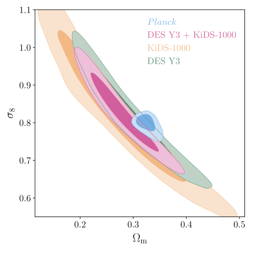
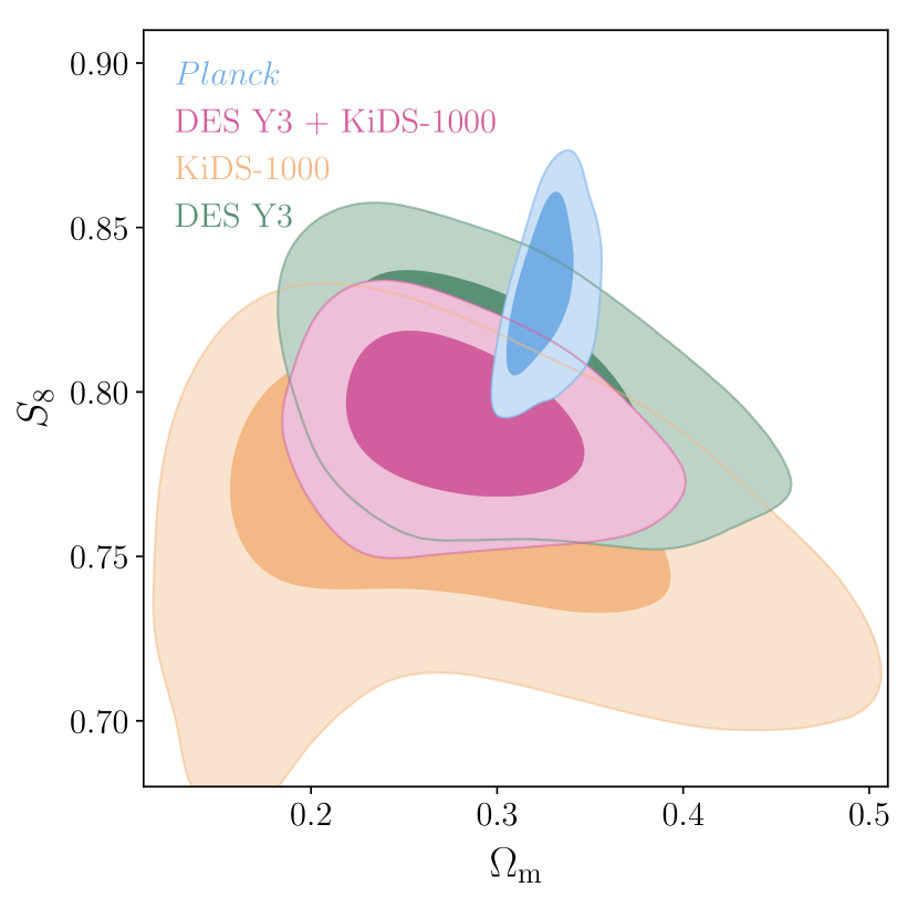
Figure 1: Cosmological constraints on the cosmological parameters $\sigma_{8}$ (left) and $S_{8}$ (right) with the matter density $\Omega_{\rm m}$ in flat-$\Lambda$CDM. We adopt a Hybrid pipeline to re-analyse cosmic shear observations from DES Y3 (green) and KiDS-1000 (yellow) and conduct a joint-survey analysis of DES Y3 + KiDS-1000 (pink). The cosmic shear constraints can be compared to a re-analysis of the Planck Collaboration (2020) CMB observations (blue) using a common set of cosmological parameters and priors. The marginalised posterior contours show the 68% (inner) and 95% (outer) credible intervals.

Our fiducial cosmic shear constraints are obtained using the Hybrid pipeline, marginalising over 6 cosmological parameters in the flat-$\Lambda$CDM model and 18 systematic and astrophysical parameters, as summarised in Tables 1 and 2. In Figure 1 we present the DES Y3 (green), KiDS-1000 (yellow) and DES Y3+KiDS-1000 (pink) cosmic shear posteriors, projected into a 2D parameter space for $\Omega_{\rm m}$, $\sigma_{8}$, and $S_{8}$. For the individual surveys, the mean marginal values of $S_{8}$, $\Omega_{\rm m}$ and $\sigma_{8}$ are found with 68% credible intervals to be

constituting 2.6% (DES Y3) and 3.5% (KiDS-1000) precision measurements of $S_{8}$. In Table 4 we report the maximum marginal and MAP+PJ-HPD statistics for $S_{8}$. This table also includes constraints from an analysis of the 8% area-cut DES Y3 data vector that is used in the joint-survey analysis. Here the overlapping region of the KiDS footprint has been excised to mitigate cross-survey covariance (see Appendix A), which we find has little impact on the DES Y3 results.

For both surveys, the model provides a good fit to the data, with a goodness of fit probability $p^{\rm DES}(\chi^{2}>\chi^{2}_{\rm min}|\nu)=0.231$ and $p^{\rm KiDS}(\chi^{2}>\chi^{2}_{\rm min}|\nu)=0.048$ (see Table 3), calculated assuming our data vector is drawn from a multivariate Gaussian likelihood and that our assumed covariance matrix is precisely and fully characterised. Before combining the two surveys we assessed their consistency. We find a DES-KiDS Hellinger distance offset in $S_{8}$ of $1.0\sigma$ (Equation 6), and a $\Delta_{\rm tension}$ parameter shift in $S_{8}-\Omega_{\rm m}$ of $0.8\sigma$ (Equation 8), thus meeting the $<2.3\sigma$ threshold for consistent data sets.

For the DES Y3+KiDS-1000 joint-survey analysis, the mean marginal values of $S_{8}$, $\Omega_{\rm m}$ and $\sigma_{8}$ and are found with 68% credible intervals to be

$$\begin{aligned} S_{8}&{}=0.790_{-0.014}^{+0.018}\\ \Omega_{\rm m}&{}=0.280^{+0.037}_{-0.046}\\ \sigma_{8}&{}=0.825^{+0.067}_{-0.073}\,,\end{aligned}$$ (11)

constituting a 2.0% precision measurement of $S_{8}$. These constraints are summarised in Figure 2 and tabulated in Table 4 including the maximum marginal and MAP+PJ-HPD values for $S_{8}$. In all cases the model is found to provide a good fit to the data (see Table 3). For our fiducial joint-survey analysis we find a goodness of fit probability $p(\chi^{2}>\chi^{2}_{\rm min}|\nu)=0.068$. We also measure the goodness of fit of the DES and KiDS data vector for the best-fit set of parameters from the joint analysis. The DES goodness of fit is essentially unchanged by the joint analysis. The KiDS goodness of fit degrades slightly, but nevertheless passes the goodness of fit requirement with $p(\chi^{2}>\chi^{2}_{\rm min}|\nu)=0.035$.

Analysis	$\chi^{2}_{\rm min}$	$N_{\Theta}$	$\chi^{2}_{\rm red}$	$p(\chi_{\rm min}^{2}|\nu_{\rm eff})$
DES Y3 (Full area)	284.2	5.4	1.06	0.231
DES Y3 (KiDS-excised)	288.3	4.6	1.07	0.192
KiDS-1000	88.3	7.1	1.30	0.048
DES Y3+KiDS-1000:
Fiducial	378.0	9.6	1.12	0.068
$\Sigma m_{\nu}=0.06{\rm eV}$	376.6	9.7	1.11	0.074
Shared IA	382.2	8.0	1.12	0.057
NLA (no z)	379.3	8.8	1.12	0.065
TATT	371.5	12.3	1.11	0.087
Dark Matter $P_{\delta}(k)$	375.5	10.2	1.11	0.076

Table 3: Goodness of fit statistics for the Hybrid pipeline: the best-fit $\chi^{2}_{\rm min}$, the estimated effective number of free parameters, $N_{\Theta}$, the reduced $\chi^{2}_{\rm red}=\chi^{2}_{\rm min}/\nu$, where $\nu$ is the number of degrees of freedom, and the goodness of fit probability $p(\chi^{2}>\chi^{2}_{\rm min}|\nu)$ (see Section 2.7). The number of data points for the DES, KiDS and joint-survey data vectors, are $N_{\rm data}=273,75,348$ respectively. The upper section reports results for the fiducial analysis of the individual and joint surveys. The lower section varies one aspect of the Hybrid joint-survey analysis: fixing the neutrino mass to $\Sigma m_{\nu}=0.06{\rm eV}$, sharing the IA parameters between the two surveys, assuming an NLA IA model without redshift evolution (no z), adopting the TATT IA model, and using a dark matter-only correction for the non-linear model of the matter power spectrum, $P_{\delta}(k)$.

Reviewing the different mean marginal, maximum marginal and MAP $S_{8}$ values in Table 4, it is worth noting that the $0.6\sigma$ offset between the MAP and mean is expected from our analysis of EuclidEmulatorv2 mocks in Appendix E.2. This offset reflects the significant skew in the marginal $S_{8}$ posterior, in addition to a potential projection effect which would arise when marginalising over a neutrino mass prior that is asymmetrical about the truth (see Appendix C.3). In the discussion that follows we quote the mean marginal values for $S_{8}$, referring the reader to Table 4 for the alternative MAP+PJ-HPD or maximum marginal metrics of the posterior.

Survey	Analysis	Mean Marginal			MAP+PJHPD			Maximum Marginal
		$S_{8}$	$\Delta S_{8}$	$\sigma/\sigma_{\rm fid}$	$S_{8}$	$\Delta S_{8}$	$\sigma/\sigma_{\rm Fid}$	$S_{8}$	$\Delta S_{8}$	$\sigma/\sigma_{\rm Fid}$
Joint	Fiducial	$0.790^{+0.018}_{-0.014}$	$0.00\sigma$	$1.00$	$0.801^{+0.011}_{-0.023}$	$0.62\sigma$	$1.06$	$0.792^{+0.017}_{-0.018}$	$0.11\sigma$	$1.09$
DES Y3	Fiducial (Full area)	$0.802^{+0.023}_{-0.019}$	$0.57\sigma$	$1.31$	$0.816^{+0.015}_{-0.028}$	$1.18\sigma$	$1.34$	$0.803^{+0.022}_{-0.021}$	$0.59\sigma$	$1.35$
DES Y3	Fiducial (KiDS-excised)	$0.806^{+0.021}_{-0.020}$	$0.74\sigma$	$1.28$	$0.803^{+0.024}_{-0.016}$	$0.64\sigma$	$1.25$	$0.807^{+0.021}_{-0.022}$	$0.76\sigma$	$1.33$
KiDS-1000	Fiducial	$0.763^{+0.031}_{-0.023}$	$-1.00\sigma$	$1.68$	$0.776^{+0.029}_{-0.027}$	$-0.53\sigma$	$1.73$	$0.770^{+0.026}_{-0.031}$	$-0.71\sigma$	$1.77$
Joint	$\Sigma m_{\nu}=0.06$eV	$0.797^{+0.017}_{-0.014}$	$0.39\sigma$	$0.98$	$0.798^{+0.019}_{-0.014}$	$0.49\sigma$	$1.02$	$0.798^{+0.016}_{-0.018}$	$0.47\sigma$	$1.04$
Joint	Shared IA	$0.792^{+0.018}_{-0.013}$	$0.09\sigma$	$0.98$	$0.804^{+0.015}_{-0.020}$	$0.75\sigma$	$1.09$	$0.795^{+0.016}_{-0.018}$	$0.25\sigma$	$1.06$
Joint	NLA (no-z)	$0.792^{+0.016}_{-0.014}$	$0.08\sigma$	$0.94$	$0.788^{+0.020}_{-0.010}$	$-0.19\sigma$	$0.93$	$0.791^{+0.017}_{-0.015}$	$0.02\sigma$	$0.97$
Joint	TATT	$0.771^{+0.025}_{-0.018}$	$-0.88\sigma$	$1.35$	$0.761^{+0.024}_{-0.036}$	$-0.98\sigma$	$1.84$	$0.775^{+0.022}_{-0.023}$	$-0.66\sigma$	$1.41$
Joint	Dark Matter $P_{\delta}(k)$	$0.784^{+0.016}_{-0.015}$	$-0.42\sigma$	$0.95$	$0.785^{+0.014}_{-0.016}$	$-0.36\sigma$	$0.93$	$0.786^{+0.015}_{-0.016}$	$-0.30\sigma$	$0.97$
Planck	Fiducial	$0.831^{+0.017}_{-0.017}$		$1.04$	$0.834^{+0.019}_{-0.017}$		$1.09$	$0.831^{+0.018}_{-0.018}$		$1.10$
Planck	$\Sigma m_{\nu}=0.06$eV	$0.835^{+0.015}_{-0.016}$		$0.97$	$0.838^{+0.013}_{-0.019}$		$0.98$	$0.837^{+0.014}_{-0.018}$		$1.02$

Table 4: $S_{8}$ constraints with 68% credible intervals using the mean 1D marginal posterior, the MAP and PJ-HPD, and the maximum 1D marginal. Constraints are provided for our fiducial analysis of DES Y3, KiDS-1000 and the joint-survey analysis. We also report constraints from a series of analysis variants which, in descending order, adopt a fixed neutrino mass, a shared set of intrinsic alignment parameters for the two surveys, an NLA analysis with no redshift evolution fixing $\eta_{\rm IA}=0$, a TATT intrinsic alignment model analysis and a dark matter only analysis with no marginalisation over the effects of baryonic feedback. $\Delta S_{8}$ quantifies the offset of each statistic’s value for $S_{8}$ relative to the Hybrid joint analysis, mean marginal value $S_{8}^{\rm Fid}=0.790$, as a fraction of the $1\sigma$ error for each statistic. The error is also tabulated as a ratio to the fiducial joint analysis error $\sigma_{\rm Fid}=0.016$. The cosmic shear constraints can be compared to a reanalysis of the Planck Collaboration (2020) CMB observations (see Section 3.5 for details) using the Hybrid pipeline’s set of cosmological parameter priors with a free neutrino mass density, or a fixed neutrino mass prior with $\Sigma m_{\nu}=0.06$eV. We do not list $\Delta S_{8}$ for the Planck constraints, referring the reader to Section 3.5 for a more appropriate set of metrics to compare independent cosmological probes.

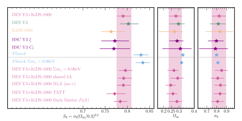
Figure 2: Summary of mean marginalised 1D constraints on $S_{8}$, $\Omega_{\rm m}$ and $\sigma_{8}$. The mean of the posterior is indicated by the filled symbol and 68% credible intervals are shown as horizontal bars. The DES and KiDS Hybrid analyses are represented as the yellow and green stars, respectively, and the joint Hybrid analysis as the pink star and vertical shaded region. Variants of the joint Hybrid analyses are shown as pink diamonds. In descending order, we show variants adopting a fixed neutrino mass, a shared set of intrinsic alignment parameters for the two surveys, an NLA analysis with no redshift evolution fixing $\eta_{\rm IA}=0$, a TATT intrinsic alignment model analysis and a dark matter only analysis with no marginalisation over the effects of baryonic feedback. The DES and KiDS constraints can be compared to a Hybrid pipeline re-analysis of the HSC Year 3 cosmic shear observations (purple stars) using the shear angular power spectrum, $C_{\ell}$, (Dalal et al., 2023) and the two-point shear correlation function, $\xi_{\pm}(\theta)$ (Li et al., 2023a, see Section 3.7 for details). We also compare to a reanalysis of the Planck Collaboration (2020) CMB observations (see Section 3.5 for details) using the Hybrid pipeline’s set of cosmological parameter priors with a free neutrino mass density (blue star), or a fixed neutrino mass prior with $\Sigma m_{\nu}=0.06$eV (blue diamond). The numerical parameter values for $S_{8}$ are listed in Table 4.

3.2 Fixing the neutrino mass density

In our fiducial analysis we allow the neutrino mass density to vary. Following Planck Collaboration (2020) we investigate adopting a fixed neutrino mass with $\Sigma m_{\nu}=0.06$eV, based on the minimum mass allowed by oscillation experiments when assuming a normal mass hierarchy (Capozzi et al., 2016). We find our constraints to be fairly insensitive to the choice of prior for $\Omega_{\nu}h^{2}$, similar to previous studies. Comparing the ‘DES Y3+KiDS-1000 $\Sigma m_{\nu}=0.06$eV’ analysis with the fiducial result, in Figure 2 and Table 4, we find the mean value of $S_{8}$ increases by $0.39\sigma$ and the marginal uncertainty decreases by $2\%$ with:

$$S^{\Sigma m_{\nu}=0.06{\rm eV}}_{8}=0.797^{+0.017}_{-0.014}\,.$$ (36)

In Table 4 we find that adopting a fixed neutrino mass brings the mean and maximum marginal estimates in line with the MAP. This behaviour is also seen in our mock analysis in Appendix E.2. For the fiducial Hybrid mock analysis, the offset in the marginalised $S_{8}$ constraints relative to the input truth arises from the projection of a wide and positive $\Sigma m_{\nu}$ prior, which is heavily skewed about the mock input value of $\Sigma m_{\nu}=0.06$eV.

3.3 Varying the intrinsic alignment model

In our fiducial analysis we adopt the NLA-z IA model, with two independent sets of survey-specific IA parameters: $(A^{\rm DES}_{\rm IA},\eta^{\rm DES}_{\rm IA})$ and $(A^{\rm KiDS}_{\rm IA},\eta^{\rm KiDS}_{\rm IA})$. The mean marginal constraints for these parameters are shown in Figure 3 with the DES parameters in green and the KiDS parameters in yellow. We can compare the constraints from the individual and joint-survey analyses. Analysing the surveys independently we find:

$$A^{\rm DES}_{\rm IA}=0.32^{+0.43}_{-0.37}\;\;\;\;\;A^{\rm KiDS}_{\rm IA}=0.65_{-0.54}^{+0.88}\,.$$ (37)

In a joint-survey analysis, we find $A^{\rm DES}_{\rm IA}$ reduces to accommodate a reduction in $S_{8}$ relative to the DES-only preferred value, and the same effect, but in reverse, for $A^{\rm KiDS}_{\rm IA}$:

$$A^{\rm DES,\;Joint}_{\rm IA}=-0.02_{-0.29}^{+0.58}\;\;\;\;\;A^{\rm KiDS,\;Joint}_{\rm IA}=1.04^{+0.54}_{-0.52}\,.$$ (38)

This increases the offset between the survey-preferred $A_{\rm IA}$ amplitude, but the constraints remain formally consistent with a Hellinger offset of $1.47\sigma$. As the intrinsic alignment signal is known to depend on many factors (see the discussion in Appendix C.2), we do not expect identical intrinsic alignment signals in the two surveys, hence our use of independent IA parameters. That said, as DES and KiDS have broadly similar redshift distributions and depths, with the tomographic samples dominated by fainter bluer galaxies, we do not expect considerable differences between the effective intrinsic alignment contamination of each survey. The changes to the $A_{\rm IA}$ constraints for each survey in the joint survey analysis may therefore indicate that this flexible nuisance parameter is absorbing more than just the contribution to the tomographic cosmic shear signal of intrinsically aligned galaxies. When testing a single shared set of IA parameters for the joint-analysis, we find, unsurprisingly, that the IA constraints lie between the best-fits for the two individual surveys, with $A^{\rm Shared-IA}_{\rm IA}=0.43^{+0.37}_{-0.45}$. As shown in Figure 3 with the shared-IA constraints in pink, the cosmological parameter constraints are not impacted by the choice of shared or independent IA modelling. We find negligible differences: $S_{8}$ increases by $0.1\sigma$, the marginal uncertainty decreases by $2\%$ and the goodness of fit probability decreases by $1\%$.

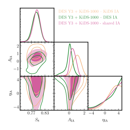
Figure 3: Constraints on the NLA-z intrinsic alignment parameters $A_{\rm IA}$ and $\eta_{\rm IA}$ with $S_{8}$. The marginalised posterior contours (inner 68% and outer 95% credible intervals) are shown for the fiducial analysis where the IA parameters are independent for the two surveys. The DES IA parameters are shown in green with the KiDS IA parameters in yellow. The fiducial result can be compared to an alternative analysis where the IA parameters are shared (pink).

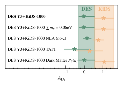
Figure 4: Summary of mean marginalised 1D constraints for the NLA-z $A_{\rm IA}$ parameter. The top row and shaded bands show the posterior mean and $1\sigma$ error bars from our fiducial Hybrid pipeline analysis of the joint DES Y3 + KiDS-1000 data vector. In descending order, we show analysis variants with fixed neutrino mass, an NLA analysis with no redshift evolution fixing $\eta_{\rm IA}=0$, a TATT intrinsic alignment model analysis and an analysis using a dark matter non-linear matter power spectrum with no marginalisation over the effects of baryonic feedback. In the case of the TATT analysis we plot constraints for the $a_{1}$ parameter, which is equal to $A_{\rm IA}$ in the limit where the TATT parameters $a_{2}$, $\eta_{2}$, $b_{\rm TA}\rightarrow 0$. See Appendix G for marginal constraints on each TATT parameter.

We are unable to constrain the redshift-dependent parameters $\eta_{\rm IA}$, but it is nevertheless interesting to note the high MAP-values for $\eta^{\rm DES,MAP}_{\rm IA}=4.5$ and $\eta^{\rm KiDS,MAP}_{\rm IA}=4.1$ which are unexpected. We find the single-survey $\eta_{\rm IA}$ posteriors also skew towards the upper edge of the $\eta_{\rm IA}$ prior, matching a similar finding in the Amon et al. (2022); Secco, Samuroff et al. (2022) DES Y3 analysis, where posteriors for the corresponding $\eta_{1}$ and $\eta_{2}$ TATT parameters also skew towards the high values allowed by the prior. This result could be indicative of the flexibility of the IA model adapting to absorb some tension in the photometric redshift evolution of the tomographic cosmic shear signals (see the discussion in Appendix C.2 and Fischbacher et al., 2023). We note, however, that as we find $S_{8}$ to be insensitive to changes in $\eta_{\rm IA}$ (see Figure 3), this result should not impact confidence in the cosmological constraints.

In our fiducial analysis we adopt the NLA-z intrinsic alignment model. Changing to the one-parameter NLA model, which removes the redshift dependence in the NLA-z framework we find negligible differences with the $S_{8}$ constraint increasing by $0.1\sigma$ and the marginal uncertainty decreasing by $6\%$ with:

$$S^{\rm NLA}_{8}=0.792^{+0.016}_{-0.013}\,.$$ (39)

As shown in Figure 4, removing freedom in the redshift evolution reduces the uncertainty on the $A_{\rm IA}$ constraints for DES and KiDS, but they remain consistent with a Hellinger offset of $1.53\sigma$.

Changing to the five-parameter TATT model (see Section 2.2), with DES-like IA priors from Table 1, we find the joint-survey cosmic shear $S_{8}$ constraint lowers by $0.9\sigma$ and the marginal uncertainty widens by $35\%$ with:

$$S^{\rm TATT}_{8}=0.771^{+0.018}_{-0.025}\,.$$ (40)

The choice for our Hybrid pipeline of NLA over TATT therefore introduces the largest impact on our results. We note that the increased uncertainty in $S_{8}$ when adopting the TATT model is in contrast to the $\sim 10\%$ reduction in uncertainty on $\Omega_{\rm m}$ and $\sigma_{8}$ (see Figure 2). Appendix G compares the multi-dimensional posteriors from the TATT and NLA-z analyses finding a similar degeneracy in the $\sigma_{8}-\Omega_{\rm m}$ plane for the two distributions, but with a significantly broader width in the case of the TATT analysis. This demonstrates that it is non-trivial to predict estimates of $S_{8}$ from the marginal distributions of $\Omega_{\rm m}$ and $\sigma_{8}$.

The trends seen here in the uncertainty and value of $S_{8}$, are similar to the trends reported by previous DES and KiDS analyses. Asgari et al. (2021) find switching from an NLA-z to a single-parameter NLA model impacts the $S_{8}$ uncertainty at the level of $\sim 10-30\%$ dependent on the two-point statistic and has a negligible impact on the value of $S_{8}$. Samuroff et al. (2019); Amon et al. (2022); Secco, Samuroff et al. (2022) find switching from NLA-z to TATT decreases $S_{8}$ by $\sim 0.6-1.0\sigma$ depending on the scale cuts, and the cosmic shear-only analysis (without shear ratio data) in Amon et al. (2022) find a $\sim 30\%$ increase in the $S_{8}$ uncertainty when adopting TATT compared to NLA-z.

To understand the differences between the NLA and TATT analyses, exploring the multi-dimensional posterior shows that the TATT IA model allows freedom for the cosmological model to explore low-$S_{8}$ values at large-$a_{2}$ values (see Appendix G). This introduces a significant skew in the marginal posterior lowering the mean $S_{8}$ value relative to the maximum marginal value. This is not only a skewness effect, however, as we find the MAP $S_{8}$ estimate is also low with $S_{8}=0.761^{+0.024}_{-0.036}$. The difference between the MAP estimates for the NLA-z and TATT analysis is $1.3\sigma$, demonstrating that the $0.9\sigma$ offset found between the mean $S_{8}$ marginals is not solely a result of prior volume or projection effects.

In our mock survey study in Appendices E.2 and C.4 we quantify the impact of adopting a TATT or NLA cosmic shear analysis for different input IA models. When the input truth model is NLA (no-z), we find a $0.45\sigma$ reduction in $S_{8}$ and a $10\%$ widening of the marginal uncertainty when changing between the Hybrid NLA-z and TATT analysis of the same simulated data vector. When the input truth model is a strong TATT model, we find a $1.3\sigma$ increase in the mean marginal $S_{8}$ value, relative to the input cosmology in an NLA-analysis. The impact of choosing TATT or NLA-z for the data lies between these two cases. At this point, with the information available to us, it is not possible to say whether the differences we find between the TATT and NLA analyses arises from a significant bias of the NLA-z model relative to the true underlying IA mechanism, or a numerical effect that will disappear as future data becomes more constraining. New observational constraints are required to help distinguish between these IA models, to set tighter priors on the free parameters, and to better inform the analysis choices for future weak lensing surveys.

3.4 Varying the baryon feedback model

In our fiducial analysis we employ two schemes to mitigate our uncertainty on the impact of baryon feedback on the non-linear matter power spectrum: scale cuts (see Appendix B) and marginalisation over the HMCode2020 $T_{\rm AGN}$ parameter (see Appendix E.2). Changing to use the HMCode2020 dark matter-only correction for the non-linear $P_{\delta}(k)$, but retaining the scale cuts, we find the joint-survey cosmic shear $S_{8}$ constraint lowers by $0.4\sigma$ and the marginal uncertainty decreases by $5\%$ with:

$$S^{\rm{Dark\,Matter}\,P_{\delta}(k)}_{8}=0.784^{+0.016}_{-0.015}\,.$$ (41)

With the inclusion of scale cuts, our constraints are therefore robust at the $0.4\sigma$-level to the use of baryon feedback marginalisation as an analysis choice. This finding is consistent with the baryon feedback sensitivity analysis in Asgari et al. (2021) and Secco, Samuroff et al. (2022) using $A_{\rm bary}$ and HMCode2016. It also matches the $0.5\sigma$ reduction in $S_{8}$ found when switching off the $T_{\rm AGN}$ marginalisation in our mock survey analysis, where the input baryon feedback was modelled using the OWLS-AGN simulation (see Appendix E.2). In Appendix G we show that we are unable to set constraints on the amplitude of the baryon feedback model.

3.5 Quantifying consistency/tension with Planck

Figure 1 compares our cosmic shear constraints to the Planck satellite CMB temperature and polarisation measurements (Planck Collaboration, 2020). Specifically we use the Planck measurements of the auto power spectra of temperature $C_{\ell}^{\rm TT}$, of $E$-modes $C_{\ell}^{\rm EE}$, and their cross-power spectra $C_{\ell}^{\rm TE}$, using the ‘Plik’ version for $\ell$ >30. In the range 2< $\ell$ <29, we only analyse the measurements of $C_{\ell}^{\rm TT}$ and $C_{\ell}^{\rm EE}$. We choose to not include the CMB lensing data that is sensitive to a wide range of redshifts, extracting cosmological information solely from the high redshift primary CMB anisotropies. In order to assess consistency, we reanalyse Planck using the Hybrid set of cosmological priors (Table 2), primarily to allow for variations in the sum of neutrino masses, a quantity which is fixed to $\Sigma m_{\nu}=0.06$eV in the fiducial Planck analysis.

The sensitivity of the CMB constraints to the choice of neutrino mass prior is shown by comparing the ‘Planck $\Sigma m_{\nu}=0.06$eV’ analysis with our Hybrid-prior re-analysis of Planck in Figure 2 and Table 4. Fixing the neutrino masses increases the Planck mean marginal $S_{8}$ value by $0.27\sigma$ with the marginal uncertainty decreasing by $10\%$.

Data	Analysis	$d_{\rm H}(S_{8})$	$\Delta_{\rm tension}^{S_{8},\Omega_{\rm m}}$
DES Y3 (Full area)	Fiducial	$1.00\sigma$	$0.87\sigma$
DES Y3 (KiDS-excised)	Fiducial	$0.90\sigma$	$0.73\sigma$
KiDS-1000	Fiducial	$2.11\sigma$	$1.89\sigma$
DES Y3 + KiDS-1000	Fiducial	$1.66\sigma$	$1.67\sigma$
DES Y3 + KiDS-1000	$\Sigma m_{\nu}=0.06$eV	$1.67\sigma$	$1.78\sigma$
DES Y3 + KiDS-1000	Shared IA	$1.57\sigma$	$1.37\sigma$
DES Y3 + KiDS-1000	NLA (no-z)	$1.67\sigma$	$1.62\sigma$
DES Y3 + KiDS-1000	TATT	$2.15\sigma$	$2.33\sigma$
DES Y3 + KiDS-1000	Dark Matter $P_{\delta}(k)$	$2.01\sigma$	$1.90\sigma$

Table 5: Tension metrics comparing the cosmological constraints from cosmic shear with those from Planck Collaboration (2020) CMB observations. We tabulate the Hellinger distance offset $d_{\rm H}(S_{8})$, and the multi-dimensional parameter shift offset $\Delta_{\rm tension}$, for the cosmic-shear constrained parameter set $(S_{8},\Omega_{\rm m})$. Metrics are reported for the fiducial Hybrid pipeline analysis of DES Y3 (both the full area and the KiDS-excised area), KiDS-1000 and the joint-survey analysis. We also report metrics for the Hybrid analysis variants where we adopt a fixed neutrino mass, a shared set of intrinsic alignment parameters for the two surveys, an NLA analysis with no redshift evolution fixing $\eta_{\rm IA}=0$, a TATT intrinsic alignment model analysis and a dark matter-only correction for the non-linear modelling of the matter power spectrum $P_{\delta}(k)$. In the case of the fixed neutrino mass analysis, we compare the cosmic shear constraint to a Planck analysis which also fixes the sum of neutrino masses to $\Sigma m_{\nu}=0.06$eV.

In Table 5 we report the Hellinger distance offset $d_{\rm H}(S_{8})$ (Equation 6) between the Hybrid pipeline cosmic shear $S_{8}$ constraints and Planck $S_{8}$ constraints. We also report the multi-dimensional parameter shift offset $\Delta_{\rm tension}$ (Equation 8) for the cosmic-shear constrained parameter set $(S_{8},\Omega_{\rm m})$, finding similar results for the two tension metrics. In all cases we find consistency between DES, KiDS and Planck. We find that the joint Hybrid constraint differs from the Planck CMB result by $1.7\sigma$, for both our fiducial setup and an analysis where the neutrino mass is fixed. The tension between the observations is driven by the KiDS survey with an $S_{8}$ Hellinger distance offset of $2.1\sigma$, compared to the DES offset of $1.0\sigma$. For our fiducial analysis we also quantify the Suspiciousness metric, Equation 10, finding a probability of $p=0.28$ to observe the measured offset between two concordant data sets. This corresponds to consistency between DES, KiDS and Planck at the level of $0.6\sigma$.

The adoption of the Hybrid pipeline reduces the previously reported tension between the DES Y3 and KiDS-1000 cosmic shear observations and Planck. In the case of KiDS, this reduction is primarily driven by an increase in the uncertainty on $S_{8}$ arising from the use of Polychord over Multinest and the inclusion of additional flexibility with the NLA-z model. In the case of DES, the reduction is primarily driven by an upward shift in $S_{8}$ which we find in our mock studies is to be expected when changing both the IA and non-linear matter power spectrum models (see Appendices C.4 and  E.2). These differences are also highlighted by the range of constraints from our variants of the Hybrid analysis. Using a TATT model increases the offset with Planck, to the level of $2.2\sigma$ (Hellinger) and $2.3\sigma$ ($\Delta_{\rm tension}$), bringing us to the limit where we would consider there to be evidence of inconsistency. Analysing the data vector with a dark matter only model for the matter power spectrum also increases the offset relative to the fiducial case, with a $2.0\sigma$ Hellinger distance offset between the joint-survey constraints and Planck.

3.6 A DES-like and KiDS-like re-analysis

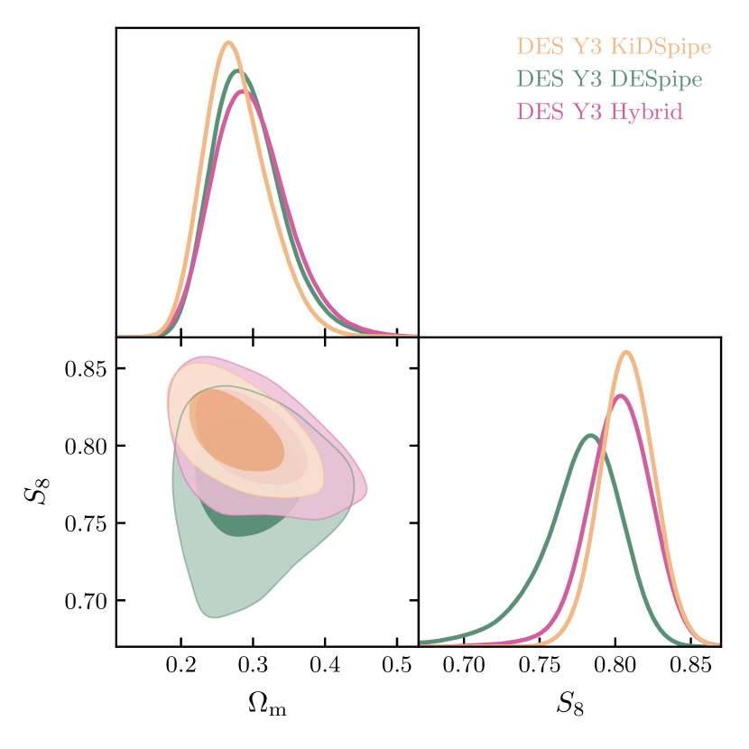
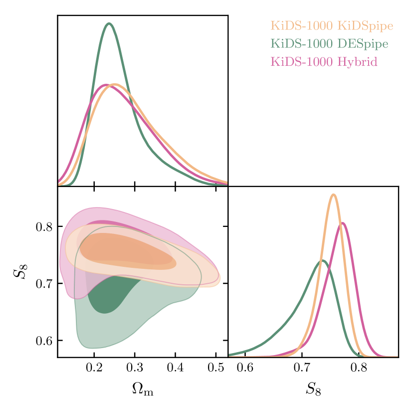
Figure 5: Cosmological constraints on $S_{8}$ and the matter density $\Omega_{\rm m}$ from DES Y3 (left) and KiDS-1000 (right): comparing our fiducial Hybrid re-analysis of the two cosmic shear surveys (pink) to analyses that adopt the original DES-like pipeline (green) and KiDS-like pipeline (yellow). The DES-like analysis of DES Y3 (green left) replicates the $\Lambda$CDM-optimised cosmic shear only constraints from Amon et al. (2022); Secco, Samuroff et al. (2022). The KiDS-like analysis of KiDS-1000 (yellow right) replicates the COSEBIs cosmic shear constraints from Asgari et al. (2021). The marginalised posterior contours show the 68% (inner) and 95% (outer) credible intervals.

In this section, we return to the original DES-like and KiDS-like pipelines, summarised in Table 2, comparing constraints with our fiducial Hybrid pipeline in the re-analysis of the DES Y3 and KiDS-1000 cosmic shear observations. Figure 5 compares constraints in the $S_{8}-\Omega_{\rm m}$ plane for DES Y3 (left) and KiDS-1000 (right), using a DES-like analysis (green), a KiDS-like analysis (yellow) and the Hybrid analysis (pink).

For both surveys, the $S_{8}$ uncertainty relative to the Hybrid analysis increases by $\sim 20\%$ for the DES-like analysis and decreases by $\sim 20\%$ for the KiDS-like analysis, in line with expectations from our mock analysis. We also see offsets between the DES-like and KiDS-like constraints for the same data set. For our re-analysis of DES Y3 we find an offset between the results from the two analysis pipelines with $\Delta S_{8}^{\rm DES}=0.033$. We can write this offset as a factor of the DES-like analysis error on $S_{8}$, with $\Delta S_{8}^{\rm DES}=1.40\sigma^{\rm DES}_{\rm DES-like}$, or as a factor of the more constraining KiDS-like analysis error on $S_{8}$, with $\Delta S_{8}^{\rm DES}=1.99\sigma^{\rm DES}_{\rm KiDS-like}$. Similar differences are seen when using the two pipelines to analyse KiDS-1000 with $\Delta S_{8}^{\rm KiDS}=0.044$. Casting this offset again as a factor of the DES-like or KiDS-like pipeline’s reported error we find $\Delta S_{8}^{\rm KiDS}=1.19\sigma^{\rm KiDS}_{\rm DES-like}=1.97\sigma^{\rm KiDS}_{\rm KiDS-like}$. In Appendices C.4 and E.2, we find that this level of offset is to be expected when analysing the same data set with the modelling combination of TATT and Halofit (DES-like) versus NLA (no-z) and HMCode (KiDS-like).

Comparing the Hybrid and KiDS-like analyses, we find similar $S_{8}$ constraints for the re-analysis of the DES survey in the left panel of Figure 5. This is expected given that the main difference for the Hybrid pipeline is the use of the Polychord sampler, in place of Multinest, with additional parameter freedoms of a varied neutrino mass and redshift-dependence in the IA modelling. These modifications are only expected to significantly impact the constraining power. In the re-analysis of the KiDS survey, however (see the right panel of Figure 5), we find a larger offset between the Hybrid and KiDS-like constraints, arising from the addition of scale cuts to the COSEBIs data vector in the Hybrid case. Appendix F examines this offset in more detail, finding a $0.7\sigma$ offset in $S_{8}$ when adopting scale cuts with an HMCode2016 KiDS-like analysis. Using a series of mocks, we show that there is a $23$% chance of such an offset arising from random shape noise. We also show that an offset of this size is unlikely to be fully attributable to small-scale baryon feedback effects using the Le Brun et al. (2014) Cosmo-OWLS:8.7 hydrodynamical simulation as an example of extreme feedback. For the KiDS-like analyses we find a DES-KiDS Hellinger distance offset in $S_{8}$ of $2.0\sigma$, and a $\Delta_{\rm tension}$ parameter shift in $S_{8}-\Omega_{\rm m}$ of $1.8\sigma$, within the $<2.3\sigma$ threshold for consistent data sets. Given that we have shown in Appendix D that the KiDS-like pipeline’s use of Multinest leads to a systematic underestimate of the constraining power, we choose to not present joint-survey constraints using the KiDS-like pipeline.

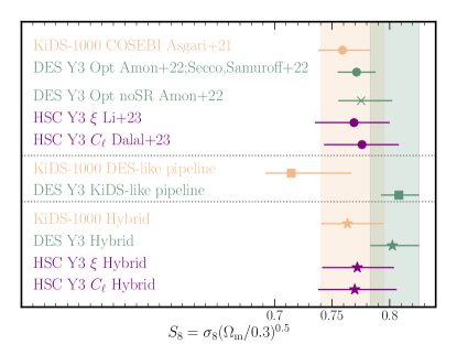
Figure 6: Constraints on $S_{8}$ from the KiDS-1000 (yellow), DES Y3 (green) and HSC Year 3 (purple) surveys, with 68% credible intervals shown as horizontal bars. In the upper section we compare the published headline results from each survey (circles). In the case of HSC we show constraints from two cosmic shear statistics, labelled $\xi_{\pm}(\theta)$ (Li et al., 2023a) and $C_{\ell}$ (Dalal et al., 2023). In the case of DES we show both the primary ‘$\Lambda$CDM optimised’ cosmic shear result from Amon et al. (2022); Secco, Samuroff et al. (2022), which includes additional shear ratio data (green circle), and the cosmic shear-only constraint (‘no SR’, green cross). In the middle section we present constraints from a DES-like re-analysis of KiDS-1000 (yellow square) and a KiDS-like re-analysis of DES Y3 (green square), demonstrating the differences between a TATT with Halofit analysis (DES-like) and an NLA (no-z) with HMCode2016 analysis (KiDS-like). The lower section presents the results from a unified Hybrid pipeline re-analysis of each survey (stars), along with a shaded vertical bar for reference.

Comparing the Hybrid and DES-like analyses, we find higher $S_{8}$ values with the Hybrid setup for both surveys. This is predicted by our EuclidEmulatorv2 mock survey analysis in Appendix E where changing the non-linear power spectrum model from Halofit to HMCode2020 combined with a change in the IA model from TATT to NLA-z increases $S_{8}$ by $\sim 1\sigma$. Including a free baryon feedback parameter in the analysis raises $S_{8}$ by an additional $\sim 0.5\sigma$ when the underlying baryon feedback model is given by OWLS-AGN (see Table 12 and also Secco et al., 2022, where the impact of these analysis choices are documented for the fiducial DES Y3 analysis). In Figure 6 we show that the 34% increase in $S_{8}$ uncertainty in the DES-like re-analysis of DES Y3 compared to the headline results from Amon et al. (2022); Secco, Samuroff et al. (2022) arises from our decision to focus on a cosmic shear-only analysis, excluding the additional shear ratio data used in the original studies (denoted no SR). For the DES-like analyses we find a DES-KiDS Hellinger distance offset in $S_{8}$ of $1.2\sigma$, and a $\Delta_{\rm tension}$ parameter shift in $S_{8}-\Omega_{\rm m}$ of $0.7\sigma$, within the $<2.3\sigma$ threshold for consistent data sets. Given the offset between the recovered and input $S_{8}$ parameters in our DES-like analysis of joint-survey EuclidEmulatorv2-based mocks, however, we choose to not present joint-survey constraints using the DES-like pipeline. In our conclusions, we discuss the implications of these differences for future survey analyses.

3.7 A comparison of constraints with HSC Year 3

In Figure 6 we compare the DES Y3 and KiDS-1000 $S_{8}$ constraints to the cosmic shear analysis of HSC Year 3 data (Li et al., 2022). The upper section presents the headline HSC results from the two-point shear correlation function analysis, $\xi_{\pm}(\theta)$ (Li et al., 2023a), and the shear angular power spectrum analysis, $C^{\rm EE}_{\epsilon\epsilon}(\ell)$ (Dalal et al., 2023). These results are in good agreement with the headline results from DES Y3 and KiDS-1000. As demonstrated throughout this paper, however, caution is required when comparing headline results as the offsets induced by different analysis choices can be significant.

We compare the HSC Year 3 fiducial analysis choices to the Hybrid approach adopted in this study. Both analyses use the Polychord sampler and to mitigate the impact of baryon feedback, both analyses incorporate scale cuts and model-marginalisation with a free nuisance parameter. The HSC team uses HMCode2016 for their headline result, however, in contrast to the Hybrid choice of HMCode2020. The HSC team chooses TATT for their IA model, in contrast to NLA-z. The $A_{\rm s}$ parameter is chosen to sample over, along with the inclusion of a correction weight (Sugiyama et al., 2020), in contrast to the $S_{8}$ parameter sampling chosen in the Hybrid setup. The HSC team also choose to fix the sum of the neutrino masses to $\Sigma m_{\nu}=0.06$eV. The projection effects and impact of each of these analysis choices is quantified in detail in Dalal et al. (2023); Li et al. (2023a), finding any offsets induced in $S_{8}$ are less than $\sim 0.5\sigma$.

In the lower section of Figure 6, we compare DES Y3, HSC Year 3 and KiDS-1000 $S_{8}$ constraints analysed with the same Hybrid pipeline and reported using mean marginal values. As in the cases of DES and KiDS, in the Hybrid re-analysis of HSC we preserve the observational calibration parameters determined by the survey. We discuss the differences between the published and Hybrid DES and KiDS results in Section 3.6. For HSC Year 3 we find little impact on the reported constraints when adopting the Hybrid pipeline in place of the HSC fiducial analysis pipeline. In contrast to the DES+KiDS joint-survey analysis in Section 3.3, a significant offset is not seen in the HSC analysis when changing IA models from TATT to NLA-z (Dalal et al., 2023; Li et al., 2023a). The differing response to the intrinsic alignment model might be understood given the HSC team’s adoption of wide uninformative priors on the $\Delta z$ redshift calibration parameter for bins with $z_{\rm phot}>0.9$. The HSC data self-calibrates these parameters with a resulting uncertainty that is a factor of 3-9 times larger than the corresponding informative priors adopted by the DES and KiDS teams.

With a Hybrid analysis evaluated for each survey we can directly compare the results within a unified framework. The constraints are consistent between the three surveys, with all three recovering a lower value for $S_{8}$ compared to the CMB result from Planck Collaboration (2020). DES Y3 yields the tightest 2.6% precision measurement on $S_{8}$ and the highest $S_{8}$ value out of the three surveys. KiDS-1000 reports the lowest $S_{8}$ value from the set with 3.5% precision. The HSC Year 3 result lies between DES Y3 and KiDS-1000 with a 4% precision measurement. We remind the reader that as almost half of the HSC footprint overlaps with KiDS, with most of the other half overlapping with DES, these surveys are not independent.

We note that the 2% precision constraints on $S_{8}$ from our joint Hybrid analysis of DES Y3 and KiDS-1000 are less precise than the 1.6-1.9% precision constraints reported from the unified analysis of DES Y1, HSC Year 1 and KiDS-1000 by Longley et al. (2023). Excluding HSC Year 1 from their analysis, Longley et al. (2023) report a DES Y1 and KiDS-1000 $S_{8}$ precision of 2.4%. Compared to this analysis, the area of DES Y3 triples relative to DES Y1, but the resulting constraints are systematics limited. In a DES Y3-like analysis of DES Y1, Amon et al. (2022) finds the increased area leads to a $\sim 50\%$ improvement in the DES constraining power. The main differences between the Longley et al. (2023) fiducial analysis framework and the Hybrid setup include the use of the Multinest sampler and the adoption of scale cuts without marginalisation over baryon feedback. From Appendices D and E we would expect this combination of choices to decrease the Longley et al. (2023) reported uncertainty on $S_{8}$ by $\sim 20\%$ relative to a Hybrid analysis. Factoring these known differences together, we conclude that our findings are in line with those from Longley et al. (2023).

3.8 Alternative large scale structure observations

To date, the most precise constraints on $S_{8}$ come from the analysis of cosmic shear or the CMB. Other large scale structure observations also constrain this parameter including galaxy-galaxy lensing; galaxy clustering; redshift space distortions; peculiar velocities; X-ray, optical and thermal SZ cluster counts; CMB lensing; with data sometimes combined in cross-correlation or in a multi-probe analysis (see the discussion in Abdalla et al., 2022; Madhavacheril et al., 2023; Amon & Efstathiou, 2022, and references therein). In common with our constraints in Section 3.1, many results in the large scale structure literature favour $S_{8}$ values that are formally consistent, but low in comparison to Planck.

We leave a detailed comparison to other cosmological probes for future work as these results adopt a range of cosmological parameter priors which must be homogenised for a robust assessment. It is worth noting, however, the exceptions to the low-$S_{8}$ trend: the CMB lensing results from the Atacama Cosmology Telescope (ACT, Madhavacheril et al., 2023) and the South Pole Telescope (SPT, Bianchini et al., 2020). A joint analysis of ACT CMB lensing with baryon acoustic oscillation observations, finds a mean marginal value for $S_{8}=0.840\pm 0.028$, with similarly high but less constraining results from SPT. These results challenge the hypothesis that an $S_{8}$-tension exists between the Planck and large scale structure analyses as a result of a non-$\Lambda$CDM redshift evolution between the CMB early Universe prediction and direct observations of the late-time Universe. CMB lensing probes linear scales and is sensitive to structure at $0.5<z<5$ with sensitivity peaking at $z\sim 2$. This can be contrasted to cosmic shear, which probes non-linear scales and is currently sensitive to structure at $z<1$.

4 Conclusions

In a joint cosmic shear analysis of DES Y3 (Amon et al. 2022; Secco, Samuroff et al. 2022) and KiDS-1000 (Asgari et al., 2021) we find consistent cosmological constraints with CMB observations from Planck Collaboration (2020), at the $1.7\sigma$ level. We constrain cosmological parameters in flat-$\Lambda$CDM, while also varying the neutrino mass, to find a 2% fractional uncertainty on $S_{8}$, with a mean-marginal value of $S_{8}=0.790^{+0.018}_{-0.014}$ and a MAP+PJ-HPD value of $S_{8}=0.801^{+0.011}_{-0.023}$. Our results are also consistent with cosmic shear constraints from the Hyper Suprime Camera Survey (HSC, Dalal et al., 2023; Li et al., 2023a). This analysis adopts a hybrid of the DES Y3 and KiDS-1000 pipelines. Through a detailed mock analysis, comparing the impact of each modelling choice, we determine that the Hybrid pipeline is robust for the statistical power of the joint survey cosmic shear analysis. Further work will explore whether the Hybrid setup is also suitable for a $3\times 2$pt analysis.

Reflecting on two decades of cosmic shear constraints, it is clear that the significant advances made in terms of survey area have not yet been matched by dramatic improvements in constraining power. This is because with each enhancement in statistical power, as in this joint-survey analysis, it is necessary for modelling choices, nuisance parameters and priors to be re-assessed. Where there is systematic uncertainty on par with the newly reduced statistical noise, a more conservative approach must be adopted. As a result, the full statistical power of modern cosmic shear surveys has yet to be realised. In this analysis we have quantified the impact of making different analysis choices to mitigate systematics arising from astrophysical processes: intrinsic galaxy alignments, non-linear modelling of the dark matter power spectrum and the impact of baryon feedback on the total matter distribution. We have also investigated different choices for the cosmological parameter priors and samplers for the inference.

In both our mock and data studies, the most significant changes arise from the choice of IA model: NLA or TATT. Replacing our fiducial NLA-z analysis with a TATT analysis reduces the cosmological consistency with Planck to $2.2\sigma$ with the Hellinger distance metric, and $2.3\sigma$ with the parameter-shift metric $\Delta_{\rm tension}$. As such, the TATT $S_{8}$ constraints are on the borderline $2.3\sigma$ limit above which we consider there to be evidence of inconsistency. This result therefore highlights the critical importance of future research to distinguish between these IA models and others (see for example Vlah et al., 2020; Fortuna et al., 2021), better inform the parameter priors and develop alternative strategies such as a self-calibrated halo modelling approach (Asgari et al., 2023). Direct measurements of intrinsic alignments, comparing high resolution large volume hydrodynamical simulations (see for example Delgado et al., 2023) with observations from overlapping spectroscopic and imaging surveys (see for example Mandelbaum et al. 2006; Johnston, Georgiou et al. 2019; Samuroff et al. 2023) will be central to this development. Significant advances are anticipated with direct-IA analyses of the Physics of the Accelerating Universe Survey (PAUS, Johnston et al., 2021), the Dark Energy Spectroscopic Instrument Bright Galaxy Survey (DESI-BGS, Hahn et al., 2023), the Javalambre-Physics of the Accelerated Universe Astrophysical Survey (J-PAS, Benitez et al., 2014) and the 4-metre Multi-Object Spectrograph Telescope Wide Area Vista Extragalactic Survey (4-MOST WAVES, Driver et al., 2019). It may also become necessary for more complex cosmic shear studies that separate the red and blue galaxy populations to become the future standard (Heymans et al., 2013; Samuroff et al., 2019; Li et al., 2021), given that these galaxy populations exhibit clear differences in their alignment properties.

Our fiducial mitigation strategy for baryon feedback combines two complementary approaches. First, led by the findings of the BAHAMAS hydrodynamical simulations (McCarthy et al., 2017; van Daalen et al., 2020), we set a prior on the likely magnitude range for baryon feedback. Using the BAHAMAS-calibrated HMCode2020 model we then marginalise over our uncertainty on the non-linear suppression of power. Secondly, we adopt a set of scale cuts to reduce our sensitivity to baryon feedback effects, especially those that are not represented by the BAHAMAS-calibrated model and prior range. Comparing our fiducial results with an analysis that adopts a non-linear matter power spectrum with no baryon feedback, we find the $S_{8}$ constraint changes by only $0.4\sigma$. We note that these findings would likely differ, however, if we had explored more extreme feedback models which tend to raise the mean marginal value found for $S_{8}$ and decrease the overall constraining power of the analysis (Amon & Efstathiou, 2022; Preston et al., 2023). Future research is therefore essential to determine robust simulation-data comparisons and thus feedback limitations from a range of hydrodynamical simulations. The direct calibration of baryonic feedback models through mass-gas cross-correlation analyses (see for example the shear-Sunyaez Zel’dovich cross-correlation constraints from Tröster et al., 2022; Gatti et al., 2022a; Pandey et al., 2023) and galaxy-gas cross-correlation analyses (Vikram et al., 2017; Pandey et al., 2019; Koukoufilippas et al., 2019; Chiang et al., 2020; Amodeo et al., 2021; Yan et al., 2021; Schneider et al., 2022a; Sánchez et al., 2023) will also be critical if we are to robustly access cosmic shear information on scales $k>0.1h{\rm Mpc}^{-1}$ in the Euclid-Roman-Rubin era.

The choice of the non-linear matter power spectrum model and sampler are found to make less of an impact on our conclusions. In these two cases the best analysis choice for the Hybrid pipeline was, however, unambiguous. The Polychord sampler was found to accurately recover the wings of the non-Gaussian posterior. In terms of speed it is, however, significantly slower than the less accurate Multinest sampler, for our cosmic shear constraints. Future speed enhancements are likely attainable, however, with the inclusion of accurate likelihood emulators (Spurio Mancini et al., 2022). Using the large-scale high resolution suite of dark matter simulations from Euclid Collaboration: Knabenhans et al. (2021) we found 1% level accuracy in predictions of the DES and KiDS cosmic shear observables when adopting HMCode2020. Accurate recovery was found across the full emulator parameter space. Similar tests are now warranted for $3\times 2$pt studies, which are sensitive to different $k$-scales and may therefore reach different conclusions. This study should also be extended to include the recently released Aemulus $\nu$ numerical simulations (DeRose et al., 2023) which span a broad range of $\sigma_{8}$ values.

When reporting the marginalised constraints for constrained parameters, informative priors on unconstrained parameters can introduce an offset relative to the MAP, given the degeneracies between cosmological and nuisance parameters (Joachimi et al., 2021; Krause et al., 2021; Chintalapati et al., 2022). Using mock analyses, we have quantified these offsets for different sets of priors, concluding that they are significant enough to caution against the direct comparison of marginal statistics from surveys that adopt different primary parameter sets and priors (see similar conclusions from Chang et al., 2019; Joudaki et al., 2020; Longley et al., 2023). With the nuisance parameter space likely to further grow to allow for new flexibility in the modelling of astrophysical systematics, this issue is unlikely to naturally resolve. The MAP statistic is insensitive to projection effects, but with the MAP being challenging to accurately determine and a standardised method to report credible intervals around the MAP yet to be widely adopted, the MAP is traditionally underutilised. On the question of consistency or tension, we therefore encourage future studies to continue publishing chains, data vectors, covariances and software to allow for the homogenisation of priors in comparison analyses and the subsequent direct comparison of posteriors, rather than marginal statistics.

This is the first joint collaboration cosmic shear analysis. We have found it to be a highly productive learning experience. Previous independent cosmic shear analyses of public survey data certainly served to drive the field forward. By enabling a direct and sustained interaction between the two teams in this joint study, we found our collective understanding has been accelerated in a way that would not have been feasible from literature reviews alone. We recommend this approach to future cosmology experiments with independent but complementary teams to promote innovation and allow for the accurate comparison of results.

Author contributions

All authors contributed to this paper, to the data products, the data calibration and/or the scientific analysis and interpretation. A core team of DES and KiDS members brought together the wide body of expertise from the two survey teams along with two extensive banks of software to create the Hybrid pipeline and conduct the cosmological analysis: Alexandra Amon, Marika Asgari, Ami Choi, Catherine Heymans, Anna Porredon, Simon Samuroff and Joe Zuntz. Additional support was provided by Felipe Andrade-Oliveira, Gary Bernstein, Jonathan Blazek, Hugo Camacho, Roohi Dalal, Konrad Kuijken, Xiangchong Li, Chieh-An Lin and Jessie Muir and from the internal reviewers Chihway Chang, Scott Dodelson, Hendrik Hildebrandt and Michael Troxel.

Data and Software Availability

The DES Y3 and KiDS-1000 catalogues and data products are freely available for download. The fiducial chains from the DES Y3, KiDS-1000 and Joint analysis can be accessed at https://des.ncsa.illinois.edu/releases/y3a2/Y3key-joint-des-kids. In CosmoSIS v3.3 we include our joint survey likelihood with the example file des-y3_and_kids-1000.ini to allow for the easy reproduction of this Hybrid analysis. This version of CosmoSIS allows for $S_{8}$ sampling, the use of correlated priors for nuisance parameters, and includes a subset of the software from the Asgari COSEBIs library.

Affiliations

¹ Cerro Tololo Inter-American Observatory, NSF’s National Optical-Infrared Astronomy Research Laboratory, Casilla 603, La Serena, Chile ² Laboratório Interinstitucional de e-Astronomia - LIneA, Rua Gal. José Cristino 77, Rio de Janeiro, RJ - 20921-400, Brazil ³ Argonne National Laboratory, 9700 South Cass Avenue, Lemont, IL 60439, USA ⁴ Department of Physics, University of Michigan, Ann Arbor, MI 48109, USA ⁵ Institute of Astronomy, University of Cambridge, Madingley Road, Cambridge CB3 0HA, UK ⁶ Kavli Institute for Cosmology, University of Cambridge, Madingley Road, Cambridge CB3 0HA, UK ⁷ E.A Milne Centre, University of Hull, Cottingham Road, Hull, HU6 7RX, United Kingdom and Centre of Excellence for Data Science, AI, and Modelling (DAIM), University of Hull, Cottingham Road, Kingston-upon-Hull, HU6 7RX ⁸ Institut de Física d’Altes Energies (IFAE), The Barcelona Institute of Science and Technology, Campus UAB, 08193 Bellaterra (Barcelona) Spain ⁹ Institute of Cosmology and Gravitation, University of Portsmouth, Portsmouth, PO1 3FX, UK ¹⁰ Physics Department, 2320 Chamberlin Hall, University of Wisconsin-Madison, 1150 University Avenue Madison, WI 53706-1390 ¹¹ Department of Physics and Astronomy, University of Pennsylvania, Philadelphia, PA 19104, USA ¹² CNRS, UMR 7095, Institut d’Astrophysique de Paris, F-75014, Paris, France ¹³ Sorbonne Universités, UPMC Univ Paris 06, UMR 7095, Institut d’Astrophysique de Paris, F-75014, Paris, France ¹⁴ Center for Theoretical Physics, Polish Academy of Sciences, al. Lotników 32/46, 02-668 Warsaw, Poland ¹⁵ Department of Physics, Northeastern University, Boston, MA 02115, USA ¹⁶ University Observatory, Faculty of Physics, Ludwig-Maximilians-Universität, Scheinerstr. 1, 81679 Munich, Germany ¹⁷ Department of Physics & Astronomy, University College London, Gower Street, London, WC1E 6BT, UK ¹⁸ Argelander-Institut für Astronomie, Auf dem Hügel 71, D-53121 Bonn, Germany ¹⁹ Kavli Institute for Particle Astrophysics & Cosmology, P. O. Box 2450, Stanford University, Stanford, CA 94305, USA ²⁰ SLAC National Accelerator Laboratory, Menlo Park, CA 94025, USA ²¹ Instituto de Física Teórica, Universidade Estadual Paulista, São Paulo, Brazil ²² Department of Physics, Carnegie Mellon University, Pittsburgh, Pennsylvania 15312, USA ²³ Instituto de Astrofisica de Canarias, E-38205 La Laguna, Tenerife, Spain ²⁴ Universidad de La Laguna, Dpto. Astrofísica, E-38206 La Laguna, Tenerife, Spain ²⁵ Center for Astrophysical Surveys, National Center for Supercomputing Applications, 1205 West Clark St., Urbana, IL 61801, USA ²⁶ Department of Astronomy, University of Illinois at Urbana-Champaign, 1002 W. Green Street, Urbana, IL 61801, USA ²⁷ Institut d’Estudis Espacials de Catalunya (IEEC), 08034 Barcelona, Spain ²⁸ Institute of Space Sciences (ICE, CSIC), Campus UAB, Carrer de Can Magrans, s/n, 08193 Barcelona, Spain ²⁹ Physics Department, William Jewell College, Liberty, MO, 64068 ³⁰ Department of Astronomy and Astrophysics, University of Chicago, Chicago, IL 60637, USA ³¹ Kavli Institute for Cosmological Physics, University of Chicago, Chicago, IL 60637, USA ³² Department of Physics, Duke University Durham, NC 27708, USA ³³ NASA Goddard Space Flight Center, 8800 Greenbelt Rd, Greenbelt, MD 20771, USA ³⁴ Jodrell Bank Center for Astrophysics, School of Physics and Astronomy, University of Manchester, Oxford Road, Manchester, M13 9PL, UK ³⁵ University of Nottingham, School of Physics and Astronomy, Nottingham NG7 2RD, UK ³⁶ Hamburger Sternwarte, Universität Hamburg, Gojenbergsweg 112, 21029 Hamburg, Germany ³⁷ Department of Astrophysical Sciences, Princeton University, Princeton, NJ 08544, USA ³⁸ School of Mathematics and Physics, University of Queensland, Brisbane, QLD 4072, Australia ³⁹ Leiden Observatory, Leiden University, P.O.Box 9513, 2300RA Leiden, The Netherlands ⁴⁰ Kapteyn Astronomical Institute, University of Groningen, PO Box 800, 9700 AV Groningen, The Netherlands ⁴¹ Lawrence Berkeley National Laboratory, 1 Cyclotron Road, Berkeley, CA 94720, USA ⁴² Department of Physics, IIT Hyderabad, Kandi, Telangana 502285, India ⁴³ Fermi National Accelerator Laboratory, P. O. Box 500, Batavia, IL 60510, USA ⁴⁴ NSF AI Planning Institute for Physics of the Future, Carnegie Mellon University, Pittsburgh, PA 15213, USA ⁴⁵ Université Grenoble Alpes, CNRS, LPSC-IN2P3, 38000 Grenoble, France ⁴⁶ Ruhr University Bochum, Faculty of Physics and Astronomy, Astronomical Institute (AIRUB), German Centre for Cosmological Lensing, 44780 Bochum, Germany ⁴⁷ Department of Astronomy/Steward Observatory, University of Arizona, 933 North Cherry Avenue, Tucson, AZ 85721-0065, USA ⁴⁸ Jet Propulsion Laboratory, California Institute of Technology, 4800 Oak Grove Dr., Pasadena, CA 91109, USA ⁴⁹ Department of Physics and Astronomy, University of Waterloo, 200 University Ave W, Waterloo, ON N2L 3G1, Canada ⁵⁰ Department of Astronomy, University of California, Berkeley, 501 Campbell Hall, Berkeley, CA 94720, USA ⁵¹ Institute of Theoretical Astrophysics, University of Oslo. P.O. Box 1029 Blindern, NO-0315 Oslo, Norway ⁵² Instituto de Fisica Teorica UAM/CSIC, Universidad Autonoma de Madrid, 28049 Madrid, Spain ⁵³ Instituto de Ciencias del Cosmos (ICC), Universidad de Barcelona, Martí i Franquès, 1, 08028 Barcelona, Spain ⁵⁴ Institute for Astronomy, University of Edinburgh, Royal Observatory, Blackford Hill, Edinburgh, EH9 3HJ, UK ⁵⁵ School of Physics and Astronomy, Cardiff University, CF24 3AA, UK ⁵⁶ Department of Astronomy, University of Geneva, ch. d’Écogia 16, CH-1290 Versoix, Switzerland ⁵⁷ Santa Cruz Institute for Particle Physics, Santa Cruz, CA 95064, USA ⁵⁸ Center for Cosmology and Astro-Particle Physics, The Ohio State University, Columbus, OH 43210, USA ⁵⁹ Department of Physics, The Ohio State University, Columbus, OH 43210, USA ⁶⁰ Department of Physics, University of Arizona, Tucson, AZ 85721, USA ⁶¹ Center for Astrophysics $|$ Harvard & Smithsonian, 60 Garden Street, Cambridge, MA 02138, USA ⁶² Department of Physics and Astronomy, University College London, Gower Street, London WC1E 6BT, UK ⁶³ Department of Astrophysical Sciences, Princeton University, 4 Ivy Lane, Princeton, NJ 08544, USA ⁶⁴ Australian Astronomical Optics, Macquarie University, North Ryde, NSW 2113, Australia ⁶⁵ Lowell Observatory, 1400 Mars Hill Rd, Flagstaff, AZ 86001, USA ⁶⁶ Department of Physics, Université de Montréal, Montréal, Canada ⁶⁷ Mila - Quebec Artificial Intelligence Institute, Montréal, Canada ⁶⁸ Ciela - Montreal Institute for Astrophysical Data Analysis and Machine Learning, Montréal, Canada ⁶⁹ Center for Computational Astrophysics, Flatiron Institute, 162 5th Avenue, 10010, New York, NY, USA ⁷⁰ McWilliams Center for Cosmology, Department of Physics, Carnegie Mellon University, 5000 Forbes Ave, Pittsburgh, PA 15213, USA ⁷¹ Kavli Institute for the Physics and Mathematics of the Universe (WPI),The University of Tokyo Institutes for Advanced Study (UTIAS), The University of Tokyo, Chiba 277-8583, Japan ⁷² Instituto de Astrofísica e Ciências do Espaço, Faculdade de Ciências, Universidade de Lisboa, 1769-016 Lisboa, Portugal ⁷³ Departamento de Física Matemática, Instituto de Física, Universidade de São Paulo, CP 66318, São Paulo, SP, 05314-970, Brazil ⁷⁴ WPC Systems Ltd., 55 Qingyun Road, Tucheng, New Taipei, Taiwan ⁷⁵ Department of Applied Mathematics and Theoretical Physics, University of Cambridge, Cambridge CB3 0WA, UK ⁷⁶ George P. and Cynthia Woods Mitchell Institute for Fundamental Physics and Astronomy, and Department of Physics and Astronomy, Texas A&M University, College Station, TX 77843, USA ⁷⁷ Centro de Investigaciones Energéticas, Medioambientales y Tecnológicas (CIEMAT), Madrid, Spain ⁷⁸ Institució Catalana de Recerca i Estudis Avançats, E-08010 Barcelona, Spain ⁷⁹ Max Planck Institute for Extraterrestrial Physics, Giessenbachstrasse, 85748 Garching, Germany ⁸⁰ Perimeter Institute for Theoretical Physics, 31 Caroline St. North, Waterloo, ON N2L 2Y5, Canada ⁸¹ Department of Physics, Stanford University, 382 Via Pueblo Mall, Stanford, CA 94305, USA ⁸² School of Physics and Astronomy, Sun Yat-sen University, Guangzhou 519082, Zhuhai Campus, P.R. China ⁸³ Instituto de Física Gleb Wataghin, Universidade Estadual de Campinas, 13083-859, Campinas, SP, Brazil ⁸⁴ Observatório Nacional, Rua Gal. José Cristino 77, Rio de Janeiro, RJ - 20921-400, Brazil ⁸⁵ Kavli Institute for the Physics and Mathematics of the Universe (WPI), UTIAS, The University of Tokyo, Kashiwa, Chiba 277-8583, Japan ⁸⁶ INAF - Osservatorio Astronomico di Padova, via dell’Osservatorio 5, 35122 Padova, Italy ⁸⁷ Department of Physics, University of Genova and INFN, Via Dodecaneso 33, 16146, Genova, Italy ⁸⁸ Department of Physics and Astronomy, Pevensey Building, University of Sussex, Brighton, BN1 9QH, UK ⁸⁹ Space Telescope Science Institute, 3700 San Martin Drive, Baltimore, MD 21218, USA ⁹⁰ Shanghai Astronomical Observatory (SHAO), Nandan Road 80, Shanghai 200030, China ⁹¹ Key Laboratory of Radio Astronomy and Technology, Chinese Academy of Sciences, A20 Datun Road, Chaoyang District, Beijing, 100101, P. R. China ⁹² University of Chinese Academy of Sciences, Beijing 100049, China ⁹³ Brookhaven National Laboratory, Bldg 510, Upton, NY 11973, USA ⁹⁴ Department of Physics and Astronomy, Stony Brook University, Stony Brook, NY 11794, USA ⁹⁵ Instituto de Física, Pontificia Universidad Católica de Valparaíso, Casilla 4059, Valparaíso, Chile ⁹⁶ School of Physics and Astronomy, University of Southampton, Southampton, SO17 1BJ, UK ⁹⁷ Computer Science and Mathematics Division, Oak Ridge National Laboratory, Oak Ridge, TN 37831 ⁹⁸ Institute for Particle Physics and Astrophysics, ETH Zürich, Wolfgang-Pauli-Strasse 27, 8093 Zürich, Switzerland ⁹⁹ Institut de Recherche en Astrophysique et Planétologie (IRAP), Université de Toulouse, CNRS, UPS, CNES, 14 Av. Edouard Belin, 31400 Toulouse, France ¹⁰⁰ Excellence Cluster Origins, Boltzmannstr. 2, 85748 Garching, Germany ¹⁰¹ Universitäts-Sternwarte, Fakultät für Physik, Ludwig-Maximilians Universität München, Scheinerstr. 1, 81679 München, Germany

Appendix A Survey overlap: excising the KiDS area from the DES footprint

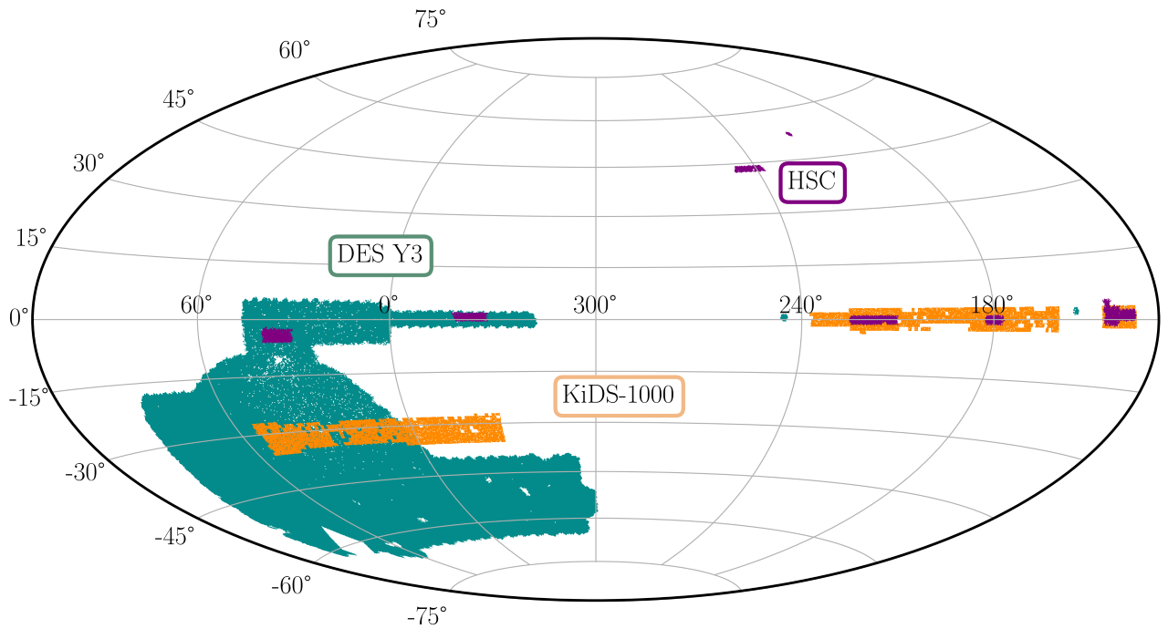
Figure 7: Survey footprints from DES Y3 (green) and KiDS-1000 (orange). The HSC-Y1 footprint (purple) overlaps KiDS in the North and DES in the South complicating the modelling of cross-survey covariance. For this reason, we limit our joint-survey analysis to DES and KiDS.

Summary: In this appendix we use simulations to estimate the cross-covariance between the DES and KiDS surveys when removing the KiDS-overlap region from the DES footprint. We conclude that the cross-covariance is sufficiently small and can therefore be neglected in the joint survey cosmic shear analysis. We confirm that the DES footprint modification, which reduces the total DES area by 8%, does not significantly impact the DES Y3 cosmological parameter constraints.

In Figure 7 we compare the DES and KiDS on-sky footprints, highlighting the Southern overlap region covering 471 square degrees, 337/246 of which are unmasked in the DES/KiDS area respectively. Data in the overlap region represents $8\%$ of DES Y3, and $32\%$ of KiDS-1000, introducing a cross-covariance between the two surveys. Given the different redshift distributions of the two surveys, it is non-trivial to analytically calculate the cross-covariance. We therefore choose to reduce the cross-covariance by excising the KiDS-overlap region from the DES survey, given the relatively smaller impact on the total DES area. We assume that DES is sufficiently homogenous that the redshift distributions are unchanged by the reduction in area. We re-measure the effective number density, the ellipticity shape noise and the mean shear and selection response, for every tomographic source bin. We find $<0.1$% changes for $\sigma_{e}$ in all bins, $<1$% changes for the mean shear response and $<1$% changes for the mean selection response in all but the second bin where the change is 2.6%. There are small changes in $n_{\rm eff}$, which is systematically higher in all bins ranging from 2% in the highest redshift source bin to 4% in the lowest redshift source bin. We then re-calculate the analytical covariance for the revised DES footprint following Friedrich et al. (2021).

In Figure 8 we compare the DES data vector from Amon et al. (2022); Secco, Samuroff et al. (2022) to the excised DES data vector and covariance that we analyse in Section 3. We find that excising the KiDS area has little impact on the DES cosmological parameter constraints with $S_{8}^{\rm original}-S_{8}^{\rm excised}=-0.0004$, using a DES-like analysis and $S_{8}^{\rm original}-S_{8}^{\rm excised}=-0.004$, using the Hybrid pipeline. The constraining power of the reduced survey area decreases when using a DES-like analysis with the 68% credible interval $\sigma_{S_{8}}^{\rm original}/\sigma_{S_{8}}^{\rm excised}=0.91$. For the Hybrid pipeline analysis, however, we find little impact on the constraining power with $\sigma_{S_{8}}^{\rm original}/\sigma_{S_{8}}^{\rm excised}=1.02$. We note these numbers will be subject to chain-to-chain variance which we expect to be at the level of $\sim 0.1\sigma$ (Joachimi et al., 2021).

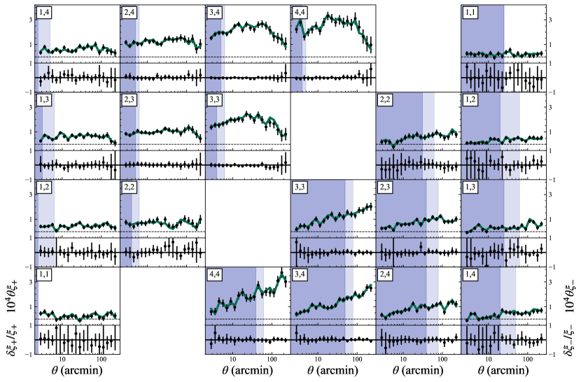
Figure 8: The DES Y3 cosmic shear two-point correlation function, $\xi_{+}(\theta)$ (left) and $\xi_{-}(\theta)$ (right), for 10 tomographic bin combinations (see label). The fiducial DES Y3 scale cuts are indicated in pale blue, with the $\Lambda$CDM-optimised scale cuts that are adopted in this cosmic shear analysis indicated in dark blue. In the upper section of each panel we compare measurements from the full DES Y3 footprint (green) and the footprint with the KiDS-overlap region excised (black) which covers 8% less area. The lower section of each panel shows the signal difference as a fraction of the best-fit theory. The analytical covariance is calculated following Friedrich et al. (2021), accounting for the reduction in area.

To assess the residual cross-survey covariance that remains after excising the overlap region, we estimate the cross-covariance from 1250 lognormal simulations created with FLASK (Xavier et al., 2016; Friedrich et al., 2021). For simplicity, we only simulate the properties of DES Y3, measuring the $\xi_{\pm}(\theta)$ statistic in 4 tomographic bins for the primary DES area where the KiDS-overlap region is excised, and the remaining DES data within the KiDS-overlap region. The additional KiDS depth and different sampling of $k$-space with the COSEBIs statistic should serve to reduce the cross-survey covariance estimated here. This analysis therefore provides an upper limit of the cross-covariance between the DES and KiDS data vectors analysed in Section 3.

Figure 9 presents the FLASK-simulation estimated joint-survey correlation matrix. We find the expected level of intra-survey covariance between the different $\xi_{+}(\theta)$ and $\xi_{-}(\theta)$ tomographic bins. For the cross-survey covariance, the majority of correlation coefficients are within a threshold of $\pm 8\%$. These levels are similar to the study in Joachimi et al. (2021) which concludes the cross-survey covariance can be neglected in a $3\times 2$pt analysis when the majority of correlation coefficients are within a threshold of $\pm 5\%$.

We follow Fang et al. (2020); Andrade-Oliveira et al. (2021) to assess the impact of neglecting cross-survey covariance through a cosmic shear $\chi^{2}$ analysis of $i=[1..500,000]$ mock joint-survey data vectors with correlated noise randomly sampled from the FLASK-estimated covariance $\bf{C}_{\rm full}$. We measure

$$\chi^{2}_{\rm A,i}=[\bf{d}_{i}-\bf{d}_{\rm th}]^{\rm T}\bf{C}_{\rm A}^{-1}[\bf{d}_{i}-\bf{d}_{\rm th}]\,,$$ (52)

where $\bf{d}_{i}$ is the data vector for realisation $i$ and $\bf{d}_{\rm th}$ is the theoretical data vector. The label A indicates the covariance matrix with A=‘full’ or A=‘no-cross’ where we zero the cross-survey blocks shown in Figure 9. We calculate $\Delta\chi^{2}_{i}=\chi^{2}_{{\rm no-cross},i}-\chi^{2}_{{\rm full},i}$ finding $\langle\Delta\chi^{2}\rangle=0\pm 11$ for $N_{\rm d}=454$ data points. These values are consistent with analytical estimates of $\Delta\chi^{2}$ from the different covariance matrices using equations 20 and 21 from Andrade-Oliveira et al. (2021). We therefore conclude that the use of an inaccurate covariance matrix that neglects cross-survey covariance will not introduce any significant effects on the inferred goodness of fit or the best-fit parameter values. Our joint-survey analysis therefore adopts a covariance matrix for the KiDS and excised-DES data vectors with zero cross-survey correlation.

Our approach differs from that of Longley et al. (2023) who account for the cross-survey covariance between KiDS and HSC in their joint cosmic shear analysis by conservatively assuming 100% correlation between the Northern stripe of KiDS and half of HSC. They then enlarge either survey’s covariance by the ratio of the full survey footprint area and the Northern footprint area. In lieu of an accurate analytical model, we find our data excision approach to be better suited for KiDS and DES, given the relatively small fractional area of DES which overlaps with KiDS. In principle, we could have adopted the same approach to also include the public HSC-Y1 catalogues into this joint-survey analysis, excising the smaller HSC-Y1 footprint from the DES equatorial stripe and KiDS-North (see Figure 7). Given that this would not increase our overall joint-survey area, however, and that the uncertainty in the $S_{8}$ constraints from this first HSC data release (Hikage et al., 2019) are $\sim 40\%$ larger than the KiDS-1000 or DES Y3 results, we choose not to extend our analysis with the inclusion of HSC-Y1. As half of the complete HSC footprint has full overlap with half of the complete KiDS footprint, any future combination of the final data releases from KiDS and HSC will require an analytical solution to account for cross-survey covariance.

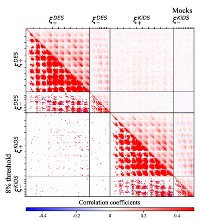
Figure 9: Correlation coefficient matrix for the DES Y3 tomographic cosmic shear data vector measured in two areas: the DES Y3 footprint with the KiDS overlap region excised, denoted $\xi_{\pm}(\theta)^{\rm DES}$, and the KiDS-excised region, denoted $\xi_{\pm}(\theta)^{\rm KiDS}$. The upper triangle shows the correlation matrix as calculated from FLASK mocks; the lower triangle shows the correlation coefficients above $\pm 8\%$. The low-levels of correlation between the main DES area and the KiDS-excised area, in the lower-left quadrants, supports our decision to neglect the cross-survey covariance between DES and KiDS in our joint-survey analysis.

Appendix B Mitigating the uncertain impact of baryon feedback with scale cuts

Summary: In this appendix we determine scale cuts for the KiDS COSEBIs data vector, following the baryon feedback mitigation strategy of Krause et al. (2021). When used in a joint-survey analysis alongside the $\Lambda$CDM-optimised scale cuts for the DES $\xi_{\pm}(\theta)$ data vector, the Hybrid pipeline is shown to be robust to the presence of baryon feedback at the level of $<0.22\sigma_{\rm 2D}$. Here $\sigma_{\rm 2D}$ is the 68% credible interval in the 2D $(S_{8},\Omega_{\rm m})$ marginalised posterior for a joint survey cosmic shear analysis.

We compare constraints in the $(S_{8},\Omega_{\rm m})$ plane between a joint-survey analysis of a mock dark-matter only and a mock van Daalen et al. (2011) OWLS-AGN baryon-feedback contaminated data vector. We then progressively remove small-scale information until the two analyses agree to within $0.3\sigma_{\rm 2D}$. We conduct this study following Krause et al. (2021) by using the DES methodology, summarised in Table 2, and adopting the best fit flat-$\Lambda$CDM cosmological parameters from Planck Collaboration (2020).

In contrast to the DES-adopted shear correlation function, $\xi_{\pm}(\theta)$, the KiDS-adopted COSEBIs statistic does not straightforwardly allow for redshift-dependent scale cuts. The theoretical prediction for each of the $E_{\rm n}$ and $B_{\rm n}$ tomographic modes is dependent on a fixed angular range $\theta_{\rm min}<\theta<\theta_{\rm max}$ (see Equation 5). Whilst predictions for varied angular ranges for each tomographic bin combination, and the corresponding analytical covariance calculation, can in principle be calculated, this approach would require an extensive update to the existing COSEBIs software. We therefore take a pragmatic approach in this study, fixing the redshift-dependent DES scale cuts to the Amon et al. (2022); Secco, Samuroff et al. (2022) defined $\Lambda$CDM-optimised scales, which predict a baryon feedback bias in a DES Y3 $\Lambda$CDM cosmic shear analysis of $<0.14\sigma_{\rm 2D}$. We then progressively increase $\theta_{\rm min}$ for the KiDS-COSEBIs analysis, in all tomographic bins, until the joint-survey analysis meets the Krause et al. (2021) robustness criteria.

For the KiDS-adopted $\theta_{\rm min}=$ 0$\stackrel{{\>{}^{\prime}}}{{\textstyle.}}$5, we do not meet the $<0.3\sigma_{\rm 2D}$ offset criteria for a KiDS-only analysis using the DES framework. We find that raising $\theta_{\rm min}=$ 2$\stackrel{{\>{}^{\prime}}}{{\textstyle.}}$0 is sufficient to mitigate the bias from OWLS-AGN baryon feedback, increasing the error on $S_{8}$ by only $\sim 10\%$. In Figure 10 we show that with this limit for KiDS, in addition to the redshift-dependent DES scale cuts from Amon et al. (2022); Secco, Samuroff et al. (2022), the Krause et al. (2021) methodology predicts a baryon feedback bias of $<0.18\sigma_{\rm 2D}$ in a DES-like joint-survey cosmic shear analysis. We note that raising $\theta_{\rm min}>$ 2$\stackrel{{\>{}^{\prime}}}{{\textstyle.}}$0 was found to significantly reduce the joint survey constraining power, without any significant reduction in the bias. For example with $\theta_{\rm min}=$5$\stackrel{{\>{}^{\prime}}}{{\textstyle.}}$0, the fractional error on $S_{8}$ increased, relative to the $\theta_{\rm min}=$ 0$\stackrel{{\>{}^{\prime}}}{{\textstyle.}}$5 case, by $\sim 30\%$, with the bias remaining at $\sim 0.2\sigma_{\rm 2D}$.

We find that this scale cut combination is also sufficient for our Hybrid set-up, using the mock analysis in Appendix E. Here we measure a baryon feedback bias for the joint cosmic shear analysis of $<0.14\sigma_{\rm 2D}$ with scale cuts alone, and $<0.22\sigma_{\rm 2D}$ for the combination of scale cuts and marginalisation over the $T_{\rm AGN}$ parameter in the HMCode2020 non-linear model. We remind the reader that these results will be subject to chain-to-chain variance. For Multinest, marginal constraints are found to differ between successive runs at the level of $\sim 0.1\sigma$ (Joachimi et al., 2021). We have not carried out a systematic analysis to quantify the level of chain-to-chain variance for Polychord, but find $\sim 0.1\sigma$ variations in the handful of Polychord chains that have been repeated in this analysis.

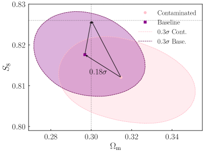
Figure 10: Cosmological constraints in the $\Omega_{\rm m}-S_{8}$ plane from a mock DES-like joint-survey analysis of data vectors from a dark-matter only Universe (‘Baseline’, purple), and an OWLS-AGN baryon-feedback contaminated Universe (‘Contaminated’, pink), for an input cosmology $\Omega_{\rm m}=0.3$ and $S_{8}=0.826$ (grey-dashed). The contours are set at $0.3\sigma_{\rm 2D}$, where $\sigma_{\rm 2D}$ is the 68% credible interval in the 2D marginalised posterior. In this analysis the KiDS COSEBIs data vector has been created with an increased minimum angular scale of $\theta_{\rm min}=$ 2$\stackrel{{\>{}^{\prime}}}{{\textstyle.}}$0, leading to an offset from the Baseline dark-matter only case of $0.18\sigma_{\rm 2D}$. We discuss the projection effects that impact both the Baseline and Contaminated analysis in Appendix C.3.

Appendix C Mock data analysis

Summary: In this appendix we quantify the impact of the different analysis choices in the DES and KiDS fiducial pipelines using a series of mock data vectors. More specifically:

• In Appendix C.1 we find that a DES-like analysis increases the $1\sigma$ uncertainty on $S_{8}$ by up to $\sim 60\%$ compared to the corresponding KiDS-like analysis of the same data set. This distinction primarily arises from the TATT or NLA choice of IA model, with little difference seen in the $S_{8}$ constraints when switching between each team’s baryon feedback mitigation strategy.

• In Appendix C.2 we review the intrinsic alignment literature, selecting survey-independent IA parameters for our fiducial analysis. We show this does not degrade the expected constraining power of the analysis.

• In Appendix C.3 we quantify projection effects in the multi-dimensional parameter space. We measure the offset of the mean and maximum value of the marginal $S_{8}$ posterior from the true input $S_{8}$ value. When using KiDS priors for a KiDS-like analysis, and DES priors for a DES-like analysis the offset introduced by projection effects on the $S_{8}$ marginal is negligible. Adopting the KiDS cosmological parameter priors for a DES-like analysis or the DES cosmological parameter priors for KiDS-like analysis, however, results in a $\sim\pm 0.5\sigma$ offset.

• In Appendix C.4 we analyse a mock data vector created with a TATT IA model and an HMCode2020 non-linear matter power spectrum with baryon feedback. In this scenario the different astrophysical modelling choices of the two teams bias the $S_{8}$ constraints in opposite directions leading to a $\sim 2\sigma$ level tension between a DES-like and a KiDS-like and analysis of the same joint-survey data vector.

Parameter	Mock Input	DES Prior	KiDS Prior
Cosmological parameters:
$10^{-9}A_{\mathrm{s}}$	2.41	$\left[0.5,\,5.0\right]$	-
$S_{8}$	$0.759$	-	$\left[0.1,1.3\right]$
$h$	0.767	$\left[0.55,0.91\right]$	$\left[0.64,0.82\right]$
$\Omega_{\mathrm{m}}$	0.246	$\left[0.1,0.9\right]$	-
$\omega_{\rm c}$	0.118	-	$\left[0.051,0.255\right]$
$\Omega_{\mathrm{b}}$	0.044	$\left[0.03,0.07\right]$	-
$\omega_{\mathrm{b}}$	0.026	-	$\left[0.019,0.026\right]$
$n_{\mathrm{s}}$	0.90	$\left[0.87,\,1.07\right]$	$\left[0.84,\,1.1\right]$
$1000\,\Omega_{\nu}h^{2}$	0.64	$\left[0.6,6.44\right]$	-
Astrophysical systematic model parameters:
TATT Intrinsic Alignments: ‘Strong’
$a_{1}$	-0.44	$\left[-5,5\right]$	-
$\eta_{1}$	4.33	$\left[-5,5\right]$	-
$a_{2}$	1.25	$\left[-5,5\right]$	-
$\eta_{2}$	2.12	$\left[-5,5\right]$	-
$b_{\rm TA}$	1.81	$\left[0,2\right]$	-
TATT Intrinsic Alignments: ‘Weak’
$a_{1}$	0.15	$\left[-5,5\right]$	-
$\eta_{1}$	-4.09	$\left[-5,5\right]$	-
$a_{2}$	-0.02	$\left[-5,5\right]$	-
$\eta_{2}$	2.31	$\left[-5,5\right]$	-
$b_{\rm TA}$	0.04	$\left[0,2\right]$	-
NLA Intrinsic Alignments:
$A_{\rm IA}$	0.26	$\left[-6,6\right]$	$\left[-6,6\right]$
Baryon Feedback:
$\log_{10}(T_{\rm AGN}/{\rm K})$	7.8	-	$\left[7.6,8.0\right]$

Table 6: Cosmological and astrophysical systematic parameters adopted for the mock survey analysis. The input parameters can be compared to the top-hat prior ranges of the DES-like and KiDS-like pipelines. The TATT ‘Strong’ parameters are the mean marginal values from the DES Y3 cosmic shear with shear ratio analysis (Amon et al. 2022; Secco, Samuroff et al. 2022). The TATT ‘Weak’ parameters are the mean marginal values from the DES Y3 $3\times 2$pt without shear ratio analysis (DES Collaboration et al., 2022). The TATT ‘Strong’ model is used to create the mocks analysed with the DES-like pipeline in Appendices C.1, C.2 and C.3. The impact of using the TATT ‘Weak’ or ‘Strong’ parameters as an input is quantified for both a DES-like and KiDS-like mock survey analysis in Appendix C.4.

This study was motivated as an alternative safety measure to a blinded data analysis, as the standard DES and KiDS blinding procedures became redundant when each survey’s result entered the public domain. Given the wide range of conclusions drawn from this mock survey analysis, we recommend that in addition to existing blinding tools, future studies use mocks to validate pipelines in both the fiducial setup (as in Joachimi et al., 2021; Krause et al., 2021), and any proposed alternative combinations of models and priors.

The suite of mock data was created using the cosmological parameters listed in Table 6 which are in agreement with both the DES Y3 and KiDS-1000 cosmic shear constraints. Specifically, we choose $S_{8}=0.759$ to match the identical reported best-fit $S_{8}$ values from the fiducial cosmic shear analysis from Amon et al. (2022); Secco, Samuroff et al. (2022), and the fiducial COSEBIs cosmic shear analysis from Asgari et al. (2021). The choice is well within $1\sigma$ of the best-fit $S_{8}$ value from the DES Y3 optimised $\Lambda$CDM cosmic shear analysis where $S_{8}=0.772^{+0.018}_{-0.017}$, and the best-fit $S_{8}$ from the KiDS-1000 band power spectra cosmic shear analysis where $S_{8}=0.760^{+0.016}_{-0.038}$.

Throughout Appendix C, when we refer to the ‘KiDS-like’ pipeline, we use the KiDS-1000 Asgari et al. (2021) pipeline with one update: the HMCode2016 non-linear model has been updated to the improved HMCode2020 model adopted in the Tröster et al. (2021) KiDS-1000 cosmic shear analysis. At the outset of this project it was our intention to only report constraints from a DES-like and KiDS-like analysis and the KiDS team wished to use the version of their pipeline that they considered to be the most accurate. They chose a $\log_{10}(T_{\rm AGN}/{\rm K})$ prior of $\left[7.6,8.0\right]$, to match the allowed baryon feedback range where BAHAMAS reproduces the observed baryon fraction at group scale. In the process of using this updated pipeline to conduct the mock survey study documented in this appendix, we appreciated the necessity to extend the scope of project and define a new Hybrid setup for our headline joint-survey results. For consistency with the most well known KiDS-1000 cosmic shear results, we chose to revert to the original Asgari et al. (2021) pipeline for the KiDS-like data analysis reported in Section 3.6. In Appendix F we find the KiDS-1000 constraints using HMCode2016 and HMCode2020 differ by $0.2\sigma$. The conclusions that we draw in this appendix are therefore also applicable to the original Asgari et al. (2021) pipeline.

In Appendices C.1, C.2 and C.3, when reporting DES-like constraints, the mock surveys have been created and analysed using Halofit, with no baryon feedback and a TATT IA model with 5 free parameters. For the same appendices, when reporting KiDS-like constraints, the mock surveys have been created and analysed using HMCode2020, including baryon feedback and an NLA IA model without redshift dependence. We choose to use a ‘noise-free’ mock data vector, such that for these mocks which match the expectation of each pipeline, the maximum a posteriori (MAP) is found at the set of input parameters. This data vector is then analysed, adopting the DES Y3, KiDS-1000 and DES Y3+KiDS-1000 cosmic shear covariances, assuming zero correlation between KiDS-1000 and DES Y3 in the joint-survey analysis.

The parameters encoded for each astrophysical systematic are listed in Table 6, as informed by the best-fit values for these parameters in Amon et al. (2022); Secco, Samuroff et al. (2022); DES Collaboration et al. (2022); Asgari et al. (2021); Tröster et al. (2021).

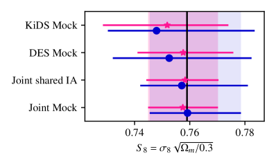
Figure 11: $S_{8}$ constraints reported from a DES-like (blue circle) and KiDS-like (pink star) analysis of mock survey data representing DES, KiDS and a joint survey. In this figure the noise-free mock survey data differs for each analysis, as they are created to match the astrophysical systematic framework within which they are analysed. For the DES-like analysis (blue), the mock surveys are created using Halofit and a TATT ‘Strong’ IA model (see Table 6). For the KiDS-like analysis (pink), the mock surveys are created using HMCode and an NLA IA model. The input cosmological model and MAP at $S_{8}=0.759$ is marked in black. Any offset in $S_{8}$ is caused by projection effects (see Appendix C.3). For the joint-survey analysis we compare an analysis where the IA nuisance parameters are shared between the surveys (Joint shared IA), to an analysis where the IA signal for each survey is considered to be independent, doubling the number of IA parameters (Joint Mock and colour bars). For the KiDS-like analysis we display the survey-preferred maximum-marginal $S_{8}$ and 68% credible intervals. For the DES-like analysis we display the survey-preferred mean-marginal $S_{8}$ and 68% credible intervals. These data are tabulated in Table 7.

Analysis	KiDS		DES
Non-linear	HMCode2020		Halofit
IA	NLA		TATT
Baryons	$T_{\rm AGN}=7.8$		Scale Cuts
Quoted $S_{8}$	Max	Mean	Max	Mean
$S_{8}^{\rm KiDS}$	$0.752^{+0.022}_{-0.023}$	$0.747^{+0.026}_{-0.017}$	$0.758^{+0.028}_{-0.033}$	$0.748^{+0.036}_{-0.018}$
$S_{8}^{\rm DES}$	$0.758^{+0.018}_{-0.017}$	$0.758^{+0.016}_{-0.017}$	$0.758^{+0.026}_{-0.028}$	$0.753^{+0.030}_{-0.020}$
$S_{8}^{\rm J1IA}$	$0.758^{+0.012}_{-0.014}$	$0.757^{+0.013}_{-0.012}$	$0.761^{+0.020}_{-0.021}$	$0.757^{+0.024}_{-0.015}$
$S_{8}^{\rm Joint}$	$0.757^{+0.013}_{-0.013}$	$0.757^{+0.011}_{-0.011}$	$0.764^{+0.016}_{-0.019}$	$0.759^{+0.019}_{-0.014}$
$\Delta S_{8}^{\rm KiDS}$	$-0.31\sigma$	$-0.55\sigma$	$-0.02\sigma$	$-0.42\sigma$
$\Delta S_{8}^{\rm DES}$	$-0.08\sigma$	$-0.04\sigma$	$-0.04\sigma$	$-0.26\sigma$
$\Delta S_{8}^{\rm J1IA}$	$-0.05\sigma$	$-0.15\sigma$	$0.10\sigma$	$-0.10\sigma$
$\Delta S_{8}^{\rm Joint}$	$-0.12\sigma$	$-0.14\sigma$	$0.27\sigma$	$0.01\sigma$
$\sigma^{\rm KiDS}/\sigma^{\rm KiDS}_{\rm min}$	$1.06$	$1.00$	$1.42$	$1.24$
$\sigma^{\rm DES}/\sigma^{\rm DES}_{\rm min}$	$1.05$	$1.00$	$1.64$	$1.53$
$\sigma^{\rm J1IA}/\sigma^{\rm J1IA}_{\rm min}$	$1.06$	$1.00$	$1.67$	$1.58$
$\sigma^{\rm Joint}/\sigma^{\rm Joint}_{\rm min}$	$1.13$	$1.00$	$1.60$	$1.48$
$\sigma^{\rm KiDS}/\sigma^{\rm Joint}$	$1.80$	$1.92$	$1.71$	$1.61$
$\sigma^{\rm DES}/\sigma^{\rm Joint}$	$1.37$	$1.47$	$1.51$	$1.52$
$\sigma^{\rm J1IA}/\sigma^{\rm Joint}$	$1.03$	$1.10$	$1.15$	$1.18$

Table 7: $S_{8}$ constraints for a DES-like and KiDS-like analysis of noise-free mock survey DES Y3 and KiDS-1000 data. In all cases the mock is created to match the non-linear, IA and baryon feedback astrophysical systematic framework within which they are analysed (see upper panel). The different rows present the results for the analysis of the KiDS, DES and Joint mocks. The columns present the results from each pipeline, reporting both the maximum-marginal $S_{8}$ (Max) and the mean-marginal $S_{8}$ (Mean) both with 68% credible intervals. $\Delta S_{8}$ quantifies the bias of the recovered $S_{8}$ relative to the true $S_{8}=0.759$, as a fraction of the $1\sigma$ error. This offset is induced by a projection effect when reporting one-dimensional marginal constraints from prior-dominated and multi-dimensional degenerate posteriors (see Appendix C.3). As the signal-to-noise of each mock data vector is identical across trials, an inspection of the relative $S_{8}$ constraining power, $\sigma^{\rm survey}/\sigma^{\rm survey}_{\rm min}$, reflects the impact of different analysis choices. Here $\sigma^{\rm survey}_{\rm min}$ is the minimum reported 68% credible interval for each mock survey across the four analysis trials (KiDS-like, DES-like, and Max and Mean defined constraints). For the joint-survey analysis we compare an analysis where the IA nuisance parameters are shared between the surveys (J1IA), to an analysis setup where the IA parameters for each survey are independent (Joint). For reference the lower section compares the constraining power for the KiDS-only, DES-only and joint shared IA analyses (J1IA), to the joint-survey analysis in each scenario. Some of this data is displayed in Figure 11.

C.1 The constraining power of a KiDS-like and DES-like cosmic shear analysis

In Table 7 and Figure 11 we present $S_{8}$ constraints from a KiDS-like and DES-like analysis of mock cosmic shear data from DES Y3, KiDS-1000 and a joint-survey analysis. We find that the DES-like constraints increase the $1\sigma$ uncertainty on $S_{8}$ by up to $\sim 60\%$ compared to the corresponding KiDS-like analysis. From the NLA-modified DES-like analysis in Table 8 and Figure 12, where the difference with the KiDS-like fiducial $S_{8}$ uncertainties is reduced to $\sim 10\%$, we can conclude that the contrast in constraining power between the KiDS and DES pipelines is mainly driven by the choice of IA model. The remaining 10% difference is likely driven by the chosen samplers, where the KiDS-chosen Multinest sampler is known to underestimate uncertainty at this level, in comparison to the DES-chosen Polychord sampler (see Appendix D and Lemos, Weaverdyck et al. 2023).

The different mitigation strategies for baryon feedback were not found to significantly impact the constraining power in the KiDS-like analysis. Table 8 and Figure 12 present constraints from a KiDS-like analysis that also adopted DES-like scale cuts to mitigate baryon feedback (see Appendix B). Given the similar results from these two analyses we can conclude that the small-scale information removed by the DES scale cuts is already being effectively removed by the baryon feedback, $T_{\rm AGN}$, nuisance parameter marginalisation in the KiDS pipeline.

Comparing the constraints from the individual mock surveys and the joint mock constraints in Table 7, we draw similar conclusions on the expected fractional gain for constraining power, irrespective of the framework used in the analysis. In the mocks we find the $1\sigma$ uncertainty on $S_{8}$ from a joint-survey analysis decreases by a factor of $1.4-1.7$ relative to KiDS-only, and a factor of $\sim 1.3$ relative to DES-shear-only. These results are replicated in our Hybrid pipeline analysis of the DES Y3, KiDS-1000 and joint-survey data in Section 3.

Joint Analysis	Modification	Maximum Marginal			Mean Marginal
		$S_{8}$	$\Delta S_{8}$	$\sigma/\sigma_{\rm min}$	$S_{8}$	$\Delta S_{8}$	$\sigma/\sigma_{\rm min}$
KiDS-like:	Fiducial	$0.758^{+0.012}_{-0.014}$	$-0.05\sigma$	$1.1$	$0.757^{+0.013}_{-0.012}$	$-0.15\sigma$	$1.0$
	with DES Priors	$0.754^{+0.013}_{-0.013}$	$-0.41\sigma$	$1.1$	$0.754^{+0.013}_{-0.012}$	$-0.43\sigma$	$1.0$
	with DES Scale cuts	$0.758^{+0.014}_{-0.013}$	$-0.11\sigma$	$1.1$	$0.758^{+0.013}_{-0.012}$	$-0.11\sigma$	$1.0$
DES-like:	Fiducial	$0.761^{+0.020}_{-0.021}$	$0.10\sigma$	$1.7$	$0.757^{+0.024}_{-0.015}$	$-0.10\sigma$	$1.6$
	with KiDS Priors	$0.770^{+0.018}_{-0.020}$	$0.58\sigma$	$1.6$	$0.766^{+0.020}_{-0.014}$	$0.39\sigma$	$1.4$
	with NLA	$0.752^{+0.013}_{-0.014}$	$-0.49\sigma$	$1.1$	$0.752^{+0.014}_{-0.013}$	$-0.49\sigma$	$1.1$
	with $\Sigma m_{\nu}=0.06{\rm eV}$	$0.772^{+0.017}_{-0.021}$	$0.68\sigma$	$1.6$	$0.766^{+0.022}_{-0.013}$	$0.42\sigma$	$1.4$

Table 8: Quantifying the impact of analysis choices in a joint mock survey analysis where the noise-free mock survey data matches the non-linear, IA and baryon feedback astrophysical systematic framework within which they are analysed. We report both the maximum-marginal $S_{8}$ and 68% credible intervals, and the mean-marginal $S_{8}$ and 68% credible intervals. $\Delta S_{8}$ quantifies the offset of the recovered $S_{8}$ from the true $S_{8}=0.759$, as a fraction of the $1\sigma$ error (see appendix C.3). The fiducial constraints from the KiDS-like and DES-like joint mock analysis can be compared to a modified analysis where the alternative set of cosmological parameter priors are adopted (as listed in Table 2). We also explore the impact of using an alternative astrophysical systematic mitigation strategy, with the KiDS-like analysis adopting scale cuts to mitigate baryon feedback (see Appendix B), and the DES-like analysis adopting the NLA model to mitigate IA. As the signal-to-noise of each mock data vector is identical for all tests, an inspection of the $S_{8}$ constraining power between the trials, $\sigma/\sigma_{\rm min}$, reflects the impact of each survey’s analysis choices. These data are displayed in Figure 12.

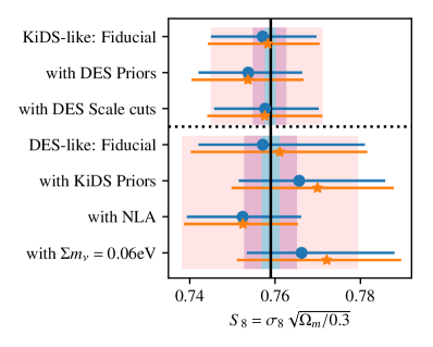
Figure 12: Mock joint-survey $S_{8}$ constraints, comparing the KiDS-like (upper section) and DES-like (lower section) fiducial analyses with modifications: adopting an alternative set of cosmological parameter priors (as listed in the second panel of Table 1); adopting alternative astrophysical systematic mitigation strategies with the KiDS-like analysis adopting scale cuts to mitigate baryon feedback (see Appendix B), and the DES-like analysis adopting the NLA model to mitigate IA. We present both the maximum-marginal $S_{8}$ and 68% credible intervals (blue circle), and the mean-marginal $S_{8}$ and 68% credible intervals (orange star). In this figure the mock data matches each survey’s chosen astrophysical systematic framework, with an identical input cosmology and signal-to-noise. For reference the colour bars show $0.1\sigma,0.3\sigma$ and $1\sigma$ bands from the fiducial analysis, centred on the input $S_{8}$, marked in black. These data are tabulated in Table 8.

C.2 Adopting shared or independent intrinsic alignment parameters

In a DES-like analysis, five nuisance parameters are used to marginalise over uncertainty in the intrinsic alignment of galaxies. In a KiDS-like analysis a single parameter is adopted (see Section 2.2 for details). In direct IA measurements significant variation is seen as a function of galaxy type and luminosity (see for example Mandelbaum et al. 2006; Johnston, Georgiou et al. 2019, and references therein). Furthermore Singh & Mandelbaum (2016); Georgiou, Johnston et al. (2019) measure a dependence of the IA amplitude on the isophote used to define galaxy ellipticity. This means that the IA nuisance parameters in our cosmic shear analyses constrain a shape-measurement dependent model of the average intrinsic alignment contamination for the source galaxy population of each survey.

Both Amon et al. (2022); Secco, Samuroff et al. (2022) and Asgari et al. (2021) measure an effective intrinsic alignment amplitude that is consistent with zero. Given the broad similarities between the DES and KiDS survey depths, redshift distributions and shape measurement approaches, we do not expect to detect any statistically significant differences between the effective intrinsic alignment contamination of the two surveys. As such, it could be preferable to adopt a single set of intrinsic alignment parameters to coherently model IA contamination in a joint-survey analysis, and we denote this approach, ‘Joint shared IA’.

It has been noted that the IA parameter constraints are somewhat sensitive to systematic errors in the photometric redshift distributions (see for example the $\lesssim 0.5\sigma$ parameter variations in Figure D.1 of Wright et al. 2020b, Figure 18 of Amon et al. 2022 and Figure 15 of Secco, Samuroff et al. 2022, when different redshift distributions are adopted in the cosmic shear analysis). Fischbacher et al. (2023) quantify the interplay between the free parameters of the IA model and photometric redshift calibration corrections which can lead to biases that are sensitive to prior volume effects. Given the differences between the DES and KiDS approach to redshift calibration, it could therefore be preferable to adopt independent sets of IA parameters, accounting for both the extra freedom that IA-marginalisation affords to absorb redshift errors and the uncertainty over the impact of variations in galaxy population and shape measurement methods. In our fiducial analyses we adopt this ‘Joint’ approach, doubling the number of IA parameters.

In Table 7 and Figure 11 we compare the two scenarios, finding the $1\sigma$ constraints on $S_{8}$ from the joint analysis to be $\sim 10\%$ smaller than the constraints from the joint shared IA analysis. This result is counter-intuitive, given that a larger number of free nuisance parameters would typically lead to a less constrained cosmological model. This behaviour is, however, not replicated in our Hybrid analysis of the data in Section 3.3 where the $S_{8}$ constraints from the shared IA analysis and fiducial joint analysis are indistinguishable. We therefore consider this unexpected result to be an artefact related to the noise-free nature of the mock data vector.

C.3 Quantifying projection effects and the offset introduced on $S_{8}$ marginals

For the mocks analysed so far in this appendix, the MAP is the input parameter set by definition, as we do not apply noise and we use priors that are either flat, or peaked at the input values. We therefore use these mocks to quantify the bias that is introduced, relative to the MAP, when reporting projected 1D marginal constraints (see also Chintalapati et al., 2022). In Table 7 and Figure 11 we compare $S_{8}$ values and their 68% credible intervals defined from the maximum-marginal, and the mean-marginal. We find that the reported maximum-marginal credible intervals are $\sim 10\%$ larger than the reported mean-marginal credible intervals for all chains. This difference is likely a result of the different approaches taken by chainconsumer and CosmoSIS-postprocess to define credible intervals (Zuntz et al., 2015; Hinton, 2016). We find a $\sim 0.2\sigma$ offset between the mean and maximum marginal for the more skewed Polychord chains that include a TATT IA model, which we discuss further in Appendix D.

In Table 8 and Figure 12 we find that the KiDS-like and DES-like fiducial joint-survey analyses recover the input cosmology within $\sim 0.1\sigma$, which is the expected run-to-run variance between chains (Joachimi et al., 2021). Interestingly, however, we find a significant offset when the alternative survey’s cosmological priors are adopted (see Table 1). In a modified KiDS-like analysis which adopts the DES cosmological priors, the reported $S_{8}$ is underestimated by $0.4\sigma$. In a modified DES-like analysis which adopts the KiDS cosmological priors, the reported $S_{8}$ is overestimated by $0.4-0.6\sigma$. Note in both these modified analyses the astrophysical systematics mitigation strategy for each survey was retained.

In order to understand the different projection effects with each survey’s choice of cosmological priors, we conducted a modified DES-like analysis using the NLA IA model, as both input to the simulated mock and as part of the analysis pipeline, and the DES cosmological priors. The resulting marginal $S_{8}$ value is underestimated by $0.5\sigma$, consistent with the bias found with a KiDS-like NLA analysis adopting DES priors. We also conducted a modified DES-like analysis adopting a fixed neutrino mass prior in addition to the other DES cosmological priors. We find the resulting marginal $S_{8}$ to be overestimated by $0.4-0.7\sigma$, similar to the bias found for a DES-like analysis which adopts the KiDS cosmological priors with a fixed neutrino mass. From these modified analyses we conclude that there is a complex interplay between the cosmological parameter priors and the astrophysical systematic prior space, especially the neutrino and IA priors. As an example of where complexity could arise we note that the non-NLA component of the TATT model, the tidal torque term modulated by the $A_{2}$ and $\eta_{2}$ parameters, depends on the linear matter power spectrum. This means that the calculated contribution to the observed cosmic shear signal from the TATT tidal torque term is insensitive to variations in the neutrino mass or the baryon feedback parameter in an inference analysis.

Chintalapati et al. (2022) show that the picture is further complicated when priors for unconstrained cosmological parameters are asymmetric about the true parameter value, as in the case of the neutrino mass prior in the DES-like analysis of these mocks. Projection effects therefore need to be carefully considered when comparing marginal statistics of surveys that adopt different primary parameter sets and priors (see for example Longley et al., 2023, who find significant shifts in poorly constrained parameters, such as $\Omega_{\rm m}$, with different prior choices).

C.4 Cosmological constraints when the underlying astrophysical model differs from the survey-specific framework

In this section we analyse mock joint-survey data where the underlying astrophysical systematic differs from the theoretical models adopted by each survey, in one way. In contrast to the mocks previously analysed, the MAP will no longer be found at the set input parameters. This study therefore quantifies potential systematic biases in the recovered cosmological parameters from a joint-survey analysis which adopts a different astrophysical systematic model from the truth. This analysis extends and complements existing studies in this area, which we briefly review before presenting the mock analysis.

In comparing IA models, Blazek et al. (2019) demonstrate that a future Rubin cosmic shear analysis that adopts the NLA IA model, when the underlying IA truth is TATT, may be subject to a significant bias in the recovered cosmological parameters. They find an offset $\Delta S_{8}\sim 0.08$ for their preferred set of TATT parameters, which would translate into a $\sim 0.7\sigma$ offset for a joint DES-KiDS analysis. Fortuna et al. (2021) reach a similar conclusion for a future Euclid-like survey cosmic shear analysis adopting the NLA IA model, when the underlying IA truth was an aligned analytical halo model. The offset they find is less significant, however, with $\Delta S_{8}\sim 0.005$, which would be negligible for this joint-survey study. Secco, Samuroff et al. (2022), analysing mock DES Y3 cosmic shear data created with the DES Y1 best-fit TATT parameters from Samuroff et al. (2019), find a significant $\sim 3\sigma$ offset in $\Omega_{\rm m}$ with a good recovery of the input $S_{8}$ when adopting an NLA model. Campos et al. (2023) show that the different implications of these studies can be understood by recognising the strong dependence of model tests on the assumed IA parameters. Defining a range of IA models from 21 samples of the DES Y1 TATT parameter posteriors, they find bias from an NLA analysis of DES Y3-like mocks could range from $0.04\sigma_{\rm 2D}$ to $5\sigma_{\rm 2D}$, where $\sigma_{\rm 2D}$ is the 68% credible interval in the 2D $(S_{8},\Omega_{\rm m})$ marginalised posterior. They propose an empirical model selection approach to better inform the choice of IA model in future cosmic shear analyses.

Turning to the non-linear power spectrum model, Krause et al. (2021) use N-body simulations from Mira Titan, Cosmic Emu (Lawrence et al., 2017) and the EuclidEmulator1 (Euclid Collaboration: Knabenhans et al., 2019), to demonstrate that the Halofit non-linear model for the matter power spectrum is sufficiently accurate for the DES Y3 baseline $3\times 2$pt analysis with biases at $<0.15\sigma_{\rm 2D}$. They also conclude that HMCode2016 fails their requirements for a $2\times 2$pt joint galaxy-galaxy lensing and galaxy clustering analysis (see section B1 of Krause et al., 2021). In contrast, Joachimi et al. (2021) use the Cosmic Emu simulations (Heitmann et al., 2014) to demonstrate that the HMCode non-linear model for the matter power spectrum is sufficiently accurate for the KiDS-1000 baseline analysis with biases at $<0.1\sigma$ in $S_{8}$. They find, however, an unacceptable $0.3\sigma$ offset in the recovered value of $S_{8}$ when adopting Halofit. We find that these apparently inconsistent conclusions can be resolved by recognising the differing goals of the two surveys, with DES focussed on optimising the accuracy of the $3\times 2$pt analysis and KiDS more focussed on the accuracy of the cosmic shear measurement. Furthermore, a fixed tolerance level in terms of $\sigma_{\rm 2D}$ in the $\Omega_{\rm m}-S_{8}$ plane, allows for a less restricted tolerance level in the 1D $S_{8}$ marginals (see the discussion in Appendix E).

		Maximum Marginals:				Mean Marginals:
		KiDS-like:		DES-like:		KiDS-like:		DES-like:
Non-Linear	Intrinsic Alignment	$S_{8}$	$\Delta S_{8}$	$S_{8}$	$\Delta S_{8}$	$S_{8}$	$\Delta S_{8}$	$S_{8}$	$\Delta S_{8}$
Fiducial	Fiducial	$0.758^{+0.012}_{-0.014}$	$-0.05\sigma$	$0.761^{+0.020}_{-0.021}$	$0.10\sigma$	$0.757^{+0.013}_{-0.012}$	$-0.15\sigma$	$0.757^{+0.024}_{-0.015}$	$-0.10\sigma$
HMCode2020	TATT strong	$0.775^{+0.012}_{-0.012}$	$1.30\sigma$	$0.741^{+0.019}_{-0.022}$	$-0.88\sigma$	$0.775^{+0.012}_{-0.012}$	$1.28\sigma$	$0.735^{+0.024}_{-0.015}$	$-1.28\sigma$
HMCode2020	TATT weak	$0.763^{+0.012}_{-0.013}$	$0.32\sigma$	$0.736^{+0.013}_{-0.017}$	$-1.55\sigma$	$0.762^{+0.013}_{-0.013}$	$0.24\sigma$	$0.733^{+0.014}_{-0.014}$	$-1.88\sigma$

Table 9: Joint survey $S_{8}$ constraints from mock data where the underlying astrophysical systematic differs from the adopted survey-specific model. The fiducial analyses can be compared to a scenario where the non-linear matter power spectrum, including baryon feedback, is defined using HMCode2020, deviating from the Halofit model adopted by DES. The IA model is then defined using TATT, deviating from the NLA model adopted by KiDS, exploring two strengths for the TATT IA contamination (see Table 6). We report the $S_{8}$ constraints and 68% credible interval using both the maximum-marginal and mean-marginal approach, with $\Delta S_{8}$ quantifying the offset from the true $S_{8}=0.759$, as a fraction of the $1\sigma$ error. These data are displayed in Figure 13. .

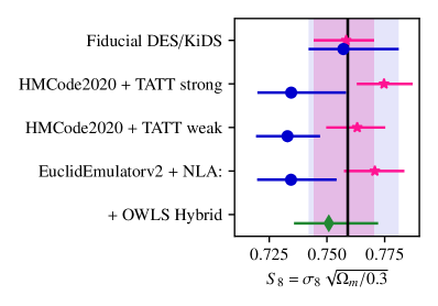
Figure 13: Joint survey $S_{8}$ constraints reported from a DES-like (blue) and KiDS-like (pink) analysis of mock survey data where the underlying astrophysical systematics differ in one way from the theoretical models adopted by each survey: the non-linear matter power spectrum, including baryon feedback, is defined using HMCode2020 as expected by the KiDS-like pipeline, and the IA contamination is defined using two different strengths of TATT as expected by the DES-like pipeline (see Table 6). For reference the colour bars show the KiDS-like (pink) and DES-like (blue) constraints from the fiducial analyses where the mocks are constructed using the astrophysical systematics expected by each pipeline. In addition, we present DES-like and KiDS-like constraints for an NLA (no-z) mock where the input power spectrum changes from an HMCode2020 model including baryon feedback, to a dark matter only EuclidEmulatorv2 model. Constraints from our Hybrid analysis are shown in green, analysing the same EuclidEmulatorv2 mock with the addition of OWLS-AGN baryon feedback. For the KiDS-like analysis we display the survey-preferred maximum-marginal $S_{8}$ and 68% credible intervals. For the DES-like and Hybrid analysis we display the survey-preferred mean-marginal $S_{8}$ and 68% credible intervals. These data are tabulated in Tables 9 and 12.

Table 9 and Figure 13 present the $S_{8}$ constraints from a DES-like and KiDS-like analysis of a joint survey cosmic shear data vector that has been created with one underlying astrophysical systematic that differs from the model adopted in each framework. The non-linear matter power spectrum is defined using HMCode2020. The baryon feedback is set with an AGN heating temperature, $\log_{10}(T_{\rm AGN}/{\rm K})=7.8$, to match the BAHAMAS simulation which best recovers the observed hot gas mass fraction of groups and clusters in addition to the galaxy stellar mass function (McCarthy et al., 2017). We include intrinsic alignments using the TATT model comparing two sets of TATT parameters. We take the best-fit TATT parameters from the optimised $\Lambda$CDM cosmic shear analysis of Amon et al. (2022); Secco, Samuroff et al. (2022), denoted TATT ‘Strong’ in Table 6. We also take the best-fit TATT parameters from the $3\times 2$pt analysis in DES Collaboration et al. (2022), denoted TATT ‘Weak’ in Table 6. Both of these scenarios are within the range allowed by the most constraining Y3 analysis ($3\times 2$pt with shear ratio data), and so are considered plausible given the current data.

Assessing the KiDS-like pipeline, a comparison of the fiducial analysis with the analyses from both HMCode2020+TATT mocks reveals the systematic bias in the recovered $S_{8}$ that is introduced by adopting the NLA model when the underlying truth is a DES Y3-like TATT model. The mismatch between intrinsic alignment models leads to an overestimate of the true $S_{8}$ at the level of $1.3\sigma$, in the TATT-strong case, and $0.3\sigma$ in the TATT-weak case. This result is consistent with the analysis in figure 15 of Amon et al. (2022), where the $S_{8}$ NLA constraint is $\sim 0.9\sigma$ higher than the corresponding TATT analysis. In contrast to the mock analysis of Secco, Samuroff et al. (2022), we find that the $\Omega_{\rm m}$ constraints for the HMCode2020+TATT mocks are unchanged compared to the fiducial analysis. This is in agreement with the NLA-TATT analysis comparison in Amon et al. (2022), demonstrating how sensitive the conclusions of mock studies are to the default TATT parameters adopted for the study.

Assessing the DES-like pipeline, we can compare the fiducial analysis with either of the HMCode2020+TATT mock analyses. This reveals the systematic bias in the recovered $S_{8}$ that results from adopting a Halofit non-linear correction with scale cuts to mitigate baryon feedback, when the underlying truth is a non-linear matter power spectrum from HMCode2020 including AGN baryon feedback. The mismatch between non-linear power spectrum models leads to an underestimate of the true $S_{8}$ at the level of $1.3\sigma$, in the TATT-strong case, and $1.9\sigma$ in the TATT-weak case when reporting mean marginals. As can be seen in Figure 13 the difference between these two results is primarily driven by the reduced $\sigma$ error on $S_{8}$ in the TATT-weak case. These offsets reduce to $0.9\sigma$, and $1.6\sigma$, when considering the maximum marginal constraints. Given the scale-cut analysis in Appendix B, we expect any bias from neglecting baryon feedback to be within $\sim 0.3\sigma_{\rm 2D}$. We therefore expect that this offset is primarily caused by the mismatch in the non-linear modelling of the power spectrum. We explore this further with a dark matter-only mock survey analysis in Appendix E.2.

From this mock joint survey cosmic shear analysis we conclude that neither the KiDS-like nor DES-like analysis choices pass the accuracy requirements set by each survey, when considering an $S_{8}=0.759$ cosmology with a TATT IA model and an HMCode2020 non-linear matter power spectrum. In this specific scenario, the combination of different systematic modelling choices bias the constraints in opposing directions leading to a $\sim 2\sigma$ level tension between a KiDS-like and DES-like analysis of identical data vectors. To address this potential issue we developed the concept of the Hybrid pipeline, described in Section 2, which is validated using the EuclidEmulatorv2 in Appendix E. The Hybrid setup was finalised before the joint survey data analysis commenced to minimise any confirmation bias in our decision making process.

Appendix D Sampler comparison

Summary: In this appendix we find that cosmic shear posteriors sampled with Multinest underestimate the width of the 68%/95% marginal credible interval for $S_{8}$ by 12%/15%. Polychord is shown to provide an accurate recovery, within a few percent, of both the 68% and 95% $S_{8}$ marginal credible interval when compared to a Metropolis-Hastings sampler and Emcee.

In this appendix we compare the posteriors recovered from a DES Y3 cosmic shear analysis using two nested sampling algorithms, Multinest (Feroz et al., 2009) and Polychord (Handley et al., 2015), and two Markov Chain Monte Carlo (MCMC) algorithms, Metropolis-Hastings and emcee (Metropolis et al., 1953; Goodman & Weare, 2010; Foreman-Mackey et al., 2013). Polychord and Multinest vary in their implementation of nested sampling. Multinest uses a series of multivariate ellipses to define likelihood thresholds which Lemos, Weaverdyck et al. (2023) show can lead to an undersampling of the posterior tails for many-parameter unimodal non-Gaussian posteriors. Polychord uses one-dimensional slice sampling, starting at a given set of parameter values to determine the posterior. Samples are then taken across one parameter only to find a new parameter set with a higher posterior, continuing the iteration one dimension at a time. This approach makes Polychord significantly slower than Multinest, but it was found to be more accurate in the DES Y1 lensing and clustering sampling study of Lemos, Weaverdyck et al. (2023). This appendix extends this study by analysing DES Y3 cosmic shear data from Amon et al. (2022); Secco, Samuroff et al. (2022) within the flat $\Lambda$CDM model. Our analysis duplicates and agrees with the recent HSC Y3 cosmic shear sampler comparison (Li et al., 2023a).

We adopt the DES Y3 sampler settings for Polychord, and the KiDS-1000 sampler settings for Multinest (see section 4.2 and 4.3 of Lemos, Weaverdyck et al. 2023 for details of the nested sampling hyper parameters and convergence diagnostics for each software package). To benchmark the results from these two nested samplers we use both a classical Metropolis-Hastings sampler and the emcee affine invariant MCMC sampler. Both algorithms start from a proposal distribution which we take from the output of the Multinest or Polychord analysis. We do not use these two samplers for our cosmological analysis with the Hybrid pipeline due to the lack of Bayesian evidence estimation. Furthermore, when analysing large-dimensional parameter spaces and non-Gaussian posterior distributions, the run times to reach convergence can become prohibitive.

Figure 14 shows the 68% and 95% credible intervals of the sampled posteriors, marginalised in the $\Omega_{\rm m}-S_{8}$ plane, where we have adopted the DES methodology framework summarised in Table 2. We find significant differences between the credible intervals, with a narrower Multinest posterior compared to the Polychord, emcee and Metropolis-Hastings posterior. Specifically we find the width of the 68% credible interval, $\Delta\sigma_{68}=\sigma_{68}^{\rm upper}-\sigma_{68}^{\rm lower}$, for the $S_{8}$ marginal, to be $\sim 12\%$ ($\sim 9\%$) narrower compared to the Metropolis-Hastings (emcee or Polychord) posterior (see Figure D and Table 10).

Inspecting the width of the 95% marginal credible interval, the $\sim 15\%$ narrowing of the Multinest posterior relative to the ‘truth’ is even more pronounced. The $S_{8}$ credible interval from Polychord is, however, accurate to a few percent. We note the emcee and Metropolis-Hastings analyses require a proposal distribution of starting guesses, finding a few percent variation between two analyses using initial starting points drawn from the Polychord or Multinest posteriors (see Table D for details, where Figures 14 and D display the Polychord-starting option). As such, even though we use the emcee and Metropolis-Hastings result as our ‘truth’, there is still some degree of uncertainty in it.

In Figure D we compare the 1D marginalised posteriors for $S_{8}$ for both the fiducial DES analysis which adopts the TATT IA model (upper panel), and an alternative analysis adopting the NLA (no-z) IA model (lower panel). We note that the narrowing of the posterior is asymmetrical about the maximum, which is likely a side-effect of the Multinest ellipsoidal sampling (see Figure 1 of Lemos, Weaverdyck et al. 2023 for an illustration). The skew of the Polychord $S_{8}$ posterior, relative to the Multinest posterior leads to significant differences between the lower $S_{8}$ credible interval, and larger offsets between mean $S_{8}$ marginal estimates, compared to estimates of the maximum of the marginalised $S_{8}$ posterior.

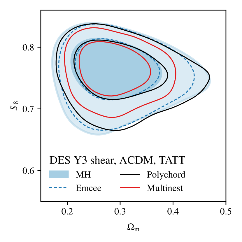
Figure 14: Comparing the Polychord (black), Multinest (red), emcee (blue, dashed) and Metropolis-Hastings (MH, light blue, filled) samplers for a DES Y3 cosmic shear analysis: the 68% and 95% credible intervals are shown for the two-dimensional posterior distribution in the $\Omega_{\rm m}-S_{8}$ plane.

Figure 15: Comparing DES Y3 cosmic shear one-dimensional marginalized posteriors for $S_{8}$ obtained using Polychord (black), Multinest (red), emcee (blue, dashed) and Metropolis-Hastings (MH, light blue) samplers. Results from an analysis using the TATT IA model, matching the posteriors shown in Figure 14, are shown in the upper row, while the lower row adopts an NLA IA model.

	$S_{8}(\rm mean)$	$\Delta\sigma_{68}$	$\Delta\sigma_{95}$
TATT:
Polychord	0.759	0.063	0.134
Multinest	0.763	0.058	0.115
emcee (PC)	0.760	0.064	0.134
emcee (MN)	0.761	0.064	0.132
Metropolis-Hastings (PC)	0.760	0.065	0.135
Metropolis-Hastings (MN)	0.760	0.067	0.137
NLA:
Polychord	0.782	0.043	0.091
Multinest	0.786	0.039	0.081

Table 10: The impact of sampler choice on one-dimensional marginalized mean $S_{8}$ constraints from the DES Y3 cosmic shear analyses. For the emcee and Metropolis-Hastings analyses, ‘PC’ and ‘MN’ indicate whether the initial starting points were drawn from the Polychord or Multinest posteriors, respectively. Columns show the CosmoSIS-postprocess-defined posterior mean, the full width of the 68% credible interval ($\Delta\sigma_{68}=\sigma_{68}^{\rm upper}-\sigma_{68}^{\rm lower}$) and the full width of the 95% credible interval ($\Delta\sigma_{95}=\sigma_{95}^{\rm upper}-\sigma_{95}^{\rm lower}$).

Appendix E Verifying the Hybrid analysis pipeline

Summary: In this appendix we quantify the accuracy of the Hybrid pipeline analysis through a series of mock analyses using the EuclidEmulatorv2 (Euclid Collaboration: Knabenhans et al., 2021).

• In Appendix E.1 we show HMCode2020 predictions of the DES $\xi_{\pm}(\theta)$ and KiDS $E_{n}$ cosmic shear observables agree with the EuclidEmulatorv2 model at the percent level across a wide range of cosmological parameters.

• In Appendix E.2 we find that using the Appendix B-defined scale cuts alone results in a $0.5\sigma$ bias on $S_{8}$ in the presence of OWLS AGN baryon feedback. Combining scale cuts with marginalisation over a free AGN feedback parameter $T_{\rm AGN}$, however, reduces the bias to $0.0\sigma$. We find the inclusion of an free neutrino mass parameter introduces a projection offset in the marginal value of $S_{8}$ at the level of $0.3\sigma$.

E.1 Quantifying the accuracy of non-linear models for DES and KiDS cosmic shear

In Figure 16 we compare the DES and KiDS cosmic shear statistics predicted from the EuclidEmulatorv2 to predictions adopting different non-linear models. The EuclidEmulatorv2 has been shown to be accurate to $<1$% for $k\lesssim 10h{\rm Mpc}^{-1}$ and $z\lesssim 3$ (Euclid Collaboration: Knabenhans et al., 2021; Adamek et al., 2023). For the mock survey analysis in this appendix we have modified our input set of cosmological parameters to lie within the emulator’s parameter range (see Table 11), retaining the input $S_{8}=0.759$, to match the fiducial $S_{8}$ cosmic shear result from both KiDS-1000 and DES Y3. With this set of cosmological parameters we find significant offsets in the small-scale cosmic shear signal when adopting Halofit.

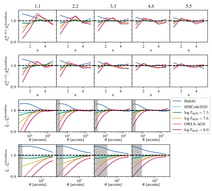
Figure 16: The ratio for a range of KiDS $E_{n}$ (upper) and DES $\xi_{\pm}(\theta)$ (lower) and cosmic shear models to the prediction from EuclidEmulatorv2. Each auto-correlation tomographic bin is shown, with similar trends found for the cross-correlations (not shown). The dark matter-only predictions for Halofit (blue) and HMCode2020 (cyan) can be compared to models that include baryon feedback using OWLS-AGN (pink) and the HMCode2020 $T_{\rm AGN}$ parameter with $\log_{10}(T_{\rm AGN}/{\rm K})=7.3$ (green), $\log_{10}(T_{\rm AGN}/{\rm K})=7.6$ (yellow) and $\log_{10}(T_{\rm AGN}/{\rm K})=8.0$ (purple). We have verified that cosmic shear signals predicted by the HMCode2020 $T_{\rm AGN}$ model (green, yellow, purple), agree at the percent level to the signals predicted when using the equivalent BAHAMAS power spectrum to directly suppress the EuclidEmulatorv2 dark matter power spectrum. The grey shaded regions indicate the adopted DES scale cuts. The upper two rows compare the KiDS fiducial COSEBIs $E_{n}$ with $\theta_{\rm min}=$ 0$\stackrel{{\>{}^{\prime}}}{{\textstyle.}}$5, to the scale cut version with $\theta_{\rm min}=$ 2$\stackrel{{\>{}^{\prime}}}{{\textstyle.}}$0.

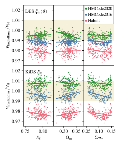
Figure 17: Comparison of the DES $\xi_{\pm}(\theta)$ (upper) and KiDS $E_{n}(\theta_{\rm min}=$0$\stackrel{{\>{}^{\prime}}}{{\textstyle.}}$5$)$ (lower) cosmic shear predictions from HMCode2020 (green), HMCode2016 (blue) and Halofit (pink), as a ratio with the prediction from the EuclidEmulatorv2 (see Equation 136) for a range of cosmological parameters. Each data point represents one sample from the DES Y3 $3\times 2$pt posterior that lies within the allowed parameter range of the EuclidEmulatorv2. The solid lines show an unweighted linear best fit to the data points as a function of input $S_{8}$ (left), $\Omega_{\rm m}$ (middle) and $\Sigma m_{\nu}$ (right). Only weak trends are seen with all the parameters including those not shown here. The shaded region brackets $\pm 1\%$ accuracy.

Parameter	Mock Input	EuclidEmulator2 range
$\Omega_{\rm b}$	$0.041$	$\left[0.04,0.06\right]$
$\Omega_{\rm m}$	$0.246$	$\left[0.24,0.40\right]$
$n_{\mathrm{s}}$	$0.99$	$\left[0.92,\,1.00\right]$
$h$	$0.7251$	$\left[0.61,0.73\right]$
$w_{0}$	$-1.0$	$\left[-1.30,-0.70\right]$
$w_{\rm a}$	$0.0$	$\left[-1.7,0.5\right]$
$\Sigma m_{\nu}$	$0.06$ eV	$\left[0.0,0.15\right]{\rm eV}$
$A_{\rm s}$	$2.445\times 10^{-9}$	$\left[1.7,2.5\right]\times 10^{-9}$

Table 11: Cosmological parameters adopted for the EuclidEmulator2-based mock joint-survey analysis which correspond to an input $S_{8}=0.759$. The chosen parameters lie within the range where the emulator has been shown to be accurate to $<1\%$ for $k\lesssim 10h{\rm Mpc}^{-1}$ and $z\lesssim 3$ (Euclid Collaboration: Knabenhans et al., 2021).

In order to determine whether the accuracy of each non-linear model changes across a wide range of cosmological parameters, in Figure 17 we compress the theoretical $\xi_{\pm}(\theta)$ or $E_{n}$ tomographic data vector, $\bf{d}$, into a single signal-to-noise estimate, $\nu$, as

$$\nu_{\rm H}=\sqrt{\bf{d}_{\rm H}^{\rm T}\,\bf{C}^{-1}\,\bf{d}_{\rm H}}\,.$$ (136)

Here $\bf{C}$ is the corresponding DES or KiDS covariance matrix and ${\rm H}$ labels the adopted non-linear model Halofit, HMCode2016 or HMCode2020. Figure 17 shows the ratio $\nu_{\rm{EuclidEmulator}}/\nu_{\rm H}$ for a range of different cosmologies that fall within the region of parameter space covered by the EuclidEmulatorv2 (see Table 11). In order to test a realistic combination of cosmological parameters, each data point represents a sample from the DES Y3 $3\times 2$pt Polychord chain. We find only weak trends with each cosmological parameter, with the HMCode2016 and HMCode2020 predictions agreeing with the EuclidEmulatorv2 model at the percent level for both statistics. Halofit provides a poorer fit, but is nevertheless accurate at the $\sim 2\%$ level overall.

Table 12 and Figure 13 present the $S_{8}$ constraints from the EuclidEmulatorv2-based mock. With the impact of the IA model choice assessed in Appendix C.4, we adopt the NLA (no-z) model as an input for this analysis. For the DES-like analysis we find an underestimate of the true $S_{8}$ at the level of $\sim 1.2\sigma$. This offset is likely caused from the mismatch between the Halofit non-linear power spectrum and EuclidEmulatorv2 shown in Figures 16 and 17, combined with the use of the TATT model which can introduce a bias in the projected marginal $S_{8}$ posterior. For the KiDS-like analysis, we find an overestimate of the true $S_{8}$ at the level of $\sim 0.9\sigma$, which can be understood when considering the $T_{\rm AGN}$ baryon feedback marginalisation within the KiDS pipeline. As shown in Figure 16, the KiDS BAHAMAS-range prior on $\log_{10}(T_{\rm AGN}/{\rm K})$, with $\left[7.6,8.0\right]$, does not allow for a dark-matter-only cosmology. It only includes feedback models which reduce power on small physical scales, such that baryon feedback marginalisation, in a dark-matter-only Universe, leads to an overestimate of the marginal $S_{8}$. In a KiDS-like analysis modified to use a dark-matter-only matter correction for the non-linear matter power spectrum, we recover an unbiased value for $S_{8}$ with $S_{8}=0.760^{+0.013}_{-0.016}$. These results lead to the same conclusion as Appendix C.4: the KiDS-like and DES-like analysis choices can lead to $\sim 2\sigma$ $S_{8}$ offsets using identical data vectors, this time when considering the scenario of an $S_{8}=0.759$ EuclidEmulatorv2-based dark-matter-only Universe.

E.2 A Hybrid pipeline analysis of EuclidEmulatorv2 mock data

EuclidEmulatorv2						Maximum Marginal			Mean Marginal
Analysis	IA	$\Sigma m_{\nu}$	+OWLS?	COSEBIs Cut?	$\log_{10}(T_{\rm AGN}/{\rm K})$	$S_{8}$	$\Delta S_{8}$	$\sigma/\sigma_{\rm min}$	$S_{8}$	$\Delta S_{8}$	$\sigma/\sigma_{\rm min}$
DES-like	TATT	free	$\times$	✓	$\times$	$0.738^{+0.017}_{-0.020}$	$-1.15\sigma$	$1.42$	$0.734^{+0.020}_{-0.015}$	$-1.44\sigma$	$1.35$
KiDS-like	NLA	0.06eV	$\times$	$\times$	$\left[7.6-8.0\right]$	$0.771^{+0.013}_{-0.013}$	$0.89\sigma$	$1.03$	$0.771^{+0.013}_{-0.013}$	$0.90\sigma$	$1.00$
A	NLA-z	0.06eV	$\times$	✓	$\times$	$0.759^{+0.017}_{-0.018}$	$0.01\sigma$	$1.36$	$0.758^{+0.016}_{-0.015}$	$-0.09\sigma$	$1.22$
B	"	"	✓	$\times$	$\times$	$0.745^{+0.017}_{-0.018}$	$-0.83\sigma$	$1.35$	$0.742^{+0.018}_{-0.013}$	$-1.10\sigma$	$1.21$
C	"	"	✓	✓	$\times$	$0.750^{+0.018}_{-0.018}$	$-0.52\sigma$	$1.42$	$0.747^{+0.019}_{-0.013}$	$-0.75\sigma$	$1.27$
D	"	"	✓	$\times$	$\left[7.6-8.0\right]$	$0.761^{+0.017}_{-0.022}$	$0.10\sigma$	$1.53$	$0.757^{+0.019}_{-0.015}$	$-0.14\sigma$	$1.33$
E	"	"	✓	✓	$\left[7.6-8.0\right]$	$0.759^{+0.019}_{-0.020}$	$-0.00\sigma$	$1.51$	$0.756^{+0.019}_{-0.015}$	$-0.16\sigma$	$1.35$
F	"	"	✓	✓	$\left[7.3-8.0\right]$	$0.759^{+0.018}_{-0.020}$	$-0.03\sigma$	$1.48$	$0.755^{+0.020}_{-0.015}$	$-0.22\sigma$	$1.39$
Hybrid	NLA-z	free	✓	✓	$\left[7.3-8.0\right]$	$0.754^{+0.020}_{-0.021}$	$-0.25\sigma$	$1.62$	$0.751^{+0.021}_{-0.015}$	$-0.46\sigma$	$1.43$
G	TATT	free	✓	✓	$\left[7.3-8.0\right]$	$0.748^{+0.022}_{-0.023}$	$-0.49\sigma$	$1.78$	$0.743^{+0.025}_{-0.015}$	$-0.81\sigma$	$1.58$

Table 12: Joint survey $S_{8}$ constraints from mock data created using the EuclidEmulatorv2 including an NLA IA model. The fiducial KiDS-like and DES-like analyses can be compared to our Hybrid pipeline. A series of tests compare the baryon feedback mitigation strategies of adopting scale cuts and/or marginalising over a free nuisance parameter $T_{\rm AGN}$ using KiDS-like priors with the addition of the NLA-z $\eta$ parameter. Where relevant, the baryon feedback is modelled using OWLS-AGN. We report the $S_{8}$ constraints and 68% credible interval using both the maximum-marginal and mean-marginal approach, with $\Delta S_{8}$ quantifying the offset from the true $S_{8}=0.759$, as a fraction of the $1\sigma$ error. Some of these data are displayed in Figure 13.

In defining a unified Hybrid pipeline it was clear that we would adopt the PolyChord sampler (Appendix D) and HMCode2020 for the non-linear power spectrum model as this outperforms both Halofit and HMCode2016 for the DES data vector in Figure 17. For the IA model choice we lack high signal-to-noise IA observations with which to make an informed decision between TATT and NLA. After discussion, the NLA-z model was selected as sufficiently complex for the signal-to-noise of our current surveys (see for example Fortuna et al., 2021). The KiDS cosmological parameter priors were then selected as these were found to minimise projection effects with the NLA model in Appendix C.3, with the addition of the DES-like prior on the NLA-z $\eta_{\rm IA}$ parameter. With these choices finalised, Tests A-F in Table 12 were designed to compare the baryon feedback mitigation strategies of adopting scale cuts and/or marginalising over a free nuisance parameter $T_{\rm AGN}$.

Starting with a mock survey that includes no baryon feedback, in Test A we recover the input $S_{8}$ within $0.1\sigma$ using only scale cuts. Test A therefore confirms the analysis in Appendix E.1 that HMCode2020 provides a sufficiently accurate description of the EuclidEmulatorv2 non-linear matter power spectrum, and the analysis in Appendix C.3 that the prior choice has minimised projection effects. In Test B and C, we quantify the impact of including scale cuts for DES and KiDS by including baryon feedback modelled through the OWLS-AGN hydrodynamical simulation (van Daalen et al., 2011) which introduces a significant reduction of power on small physical scales (see Figure 16). Adopting scale cuts for only the DES part of the joint-survey data vector (Test B) we underestimate the value of $S_{8}$ by $\sim 1.1\sigma$. Including the COSEBIs scale cuts for KiDS (Test C) reduces this bias, as designed, but we are still left with an underestimate of the value of $S_{8}$ by $\sim 0.5\sigma$ with the maximum marginal, and $\sim 0.75\sigma$ with the mean marginal. These tests may seem to contradict the analysis in Appendix B where we reported an offset of $\sim 0.14\sigma_{\rm 2D}$ in the $S_{8}-\Omega_{\rm m}$ plane for this OWLS AGN-contaminated data vector. These results can however be understood by considering the weak constraints from cosmic shear alone on $\Omega_{\rm m}$. We find that the relative error on $\Omega_{\rm m}$ is an order of magnitude larger than the relative error on $S_{8}$, such that a small bias within the $S_{8}-\Omega_{\rm m}$ plane can translate into a large relative bias in $S_{8}$. Note that the Krause et al. (2021) scale cut methodology, that we have adopted, was designed for the DES $3\times 2$pt analysis, where $\Omega_{\rm m}$ is more tightly constrained.

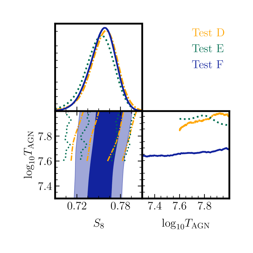
Figure 18: Comparing the degeneracy in the $S_{8}-\log_{10}(T_{\rm AGN}/{\rm K})$ plane for an analysis of noise-free EuclidEmulatorv2+OWLS-AGN mocks using different scale cuts and baryon feedback priors (see Table 12). Test D (orange, dot-dashed) applies no additional scale cuts to the KiDS mock data and shows the strongest degeneracy. Test E (green, dotted) shows that including scale cuts reduces the degeneracy. Test F (blue, solid) extends the lower bound of the $\log_{10}(T_{\rm AGN}/{\rm K})$ prior to include dark-matter only scenarios. The inner 68% and outer 95% credible intervals are shown contoured, accurately recovering the input cosmology where $S_{8}=0.759$.

In Tests D, E, and F we analyse an OWLS AGN-contaminated data vector, marginalising over the $T_{\rm AGN}$ baryon feedback parameter in HMCode2020. In all tests we recover the input $S_{8}$ within $0.2\sigma$ using the mean marginal value and within $\sim 0.1\sigma$ using the maximum marginal value. These results are expected from Figure 16 where the $T_{\rm AGN}$ prior range encompasses the OWLS-AGN model. Comparing Test D and Test E we quantify the impact of including the Appendix B-defined scale cuts to the KiDS data vector. In common with the analysis in Table 8, we find that the addition of scale cuts to KiDS does not significantly impact the $S_{8}$ constraining power, suggesting that the $T_{\rm AGN}$ marginalisation to mitigate baryon feedback is already removing the majority of information from these scales. In Figure 18 we show that the degeneracy between the baryon feedback nuisance parameter $T_{\rm AGN}$ and $S_{8}$ is, however, reduced when scale cuts are included. This is important as it implies that the scale cut analysis is less sensitive to the $T_{\rm AGN}$ prior which in this case is informative, based on our current best knowledge from hydrodynamical simulations. When expanding the informative baryon feedback prior to $\log_{10}(T_{\rm AGN}/{\rm K}):\left[7.0,10.0\right]$, Amon & Efstathiou (2022) find a $0.55\sigma$ increase in the KiDS-1000 mean marginal value for $S_{8}$ and a 40% increase in the uncertainty on that value. This study analysed the two-point shear correlation function with angular limits 0$\stackrel{{\>{}^{\prime}}}{{\textstyle.}}$5$<\theta<$ 300$\stackrel{{\>{}^{\prime}}}{{\textstyle.}}$0 for $\xi_{+}(\theta)$ and 4$\stackrel{{\>{}^{\prime}}}{{\textstyle.}}$0$<\theta<$ 300$\stackrel{{\>{}^{\prime}}}{{\textstyle.}}$0 for $\xi_{-}(\theta)$. Adopting an uninformative prior on $T_{\rm AGN}$ would further increase the uncertainty on $S_{8}$, with a stronger impact expected for statistics where the high-$k$-scale information has been removed, reducing the ability of the data to self-calibrate the baryon feedback model.

Amongst the authors there is a broad range of views on the preferred approach to mitigate baryon feedback. Those with a high degree of confidence in the scale and redshift dependence of the BAHAMAS model for baryon feedback and the HMCode2020 model for the non-linear power spectrum recommend a self-calibrating all-scale cosmic shear analysis with uninformative $T_{\rm AGN}$ priors. Those with a high degree of confidence in the BAHAMAS-defined maximum range of baryon feedback suppression, but less confidence in the finer high-$k$ details of the non-linear modelling recommend a limited scale cosmic shear analysis with informative $T_{\rm AGN}$ priors. Those with a low degree of confidence in the results from hydrodynamical simulations recommend the use of more conservative scale cuts, similar to the approach taken in Appendix B but adopting a more extreme worst case scenario for baryon feedback such as Cosmo-OWLS-AGN:8.7. Other opinions include the use of highly flexible baryon feedback models, with or without the combination of scale cuts. As we have seen in Appendix C.3, any change in prior and/or astrophysical model leads to different projection effects, some of which may be unexpected (see for example the strong degeneracy between the HMCode2016 baryon feedback parameter $A_{\rm bary}$ and $n_{\rm s}$ when using uninformative priors in Yoon & Jee, 2021). A comparison of the results from the authorship’s range of preferred baryon feedback mitigation strategies would therefore require both the analysis of mocks and data which we defer to a future study. We also note that data comparisons using different angular ranges will also be subject to random noise fluctuations (see Appendix F).

We conclude our baryon feedback study with Test F, where we expand the lower limit of the $T_{\rm AGN}$ prior to include low feedback models that are equivalent to a dark matter only model (see Figure 16). The decision to allow the non-linear model of the matter power spectrum to include no baryon feedback followed the preferred approach of Amon et al. (2022); Secco, Samuroff et al. (2022) and also Asgari et al. (2021) who allow for a dark matter only model within their baryon feedback prior. We find that extending the informative $T_{\rm AGN}$ prior to include no feedback, in combination with scale cuts, does not change the recovered $S_{8}$ value or constraining power. This can be understood from Figure 18 where we see little degeneracy between $T_{\rm AGN}$ and $S_{8}$ for $\log_{10}(T_{\rm AGN}/{\rm K})\lesssim 7.5$. For our Hybrid analysis we therefore choose to combine the mitigation strategies from both surveys using scale cuts and a $T_{\rm AGN}$ prior that spans a dark matter-only Universe through to the strongest BAHAMAS AGN feedback model.

The ‘Hybrid’ row in Table 12 repeats Test F with the Hybrid prior set, extending the KiDS prior set with the DES prior on neutrino mass. This introduces an underestimate of $S_{8}$ by $0.46\sigma$ in our recovered mean marginal $S_{8}$ value, arising from projection effects. Here our mock input neutrino mass, $\Sigma m_{\nu}=0.06$ eV, is at the lower edge of the allowed tophat prior range which extends to $\Sigma m_{\nu}<0.6$ eV. The weak correlation between $\Sigma m_{\nu}$ and $S_{8}$ then leads to a bias in the mean or maximum of the projected marginal $S_{8}$ distribution. This issue should be largely circumvented, however, by reporting the MAP in contrast to the marginal values.

In one final Test G, we replace the NLA-z model with a TATT model in our analysis to quantify the $\sim 0.8\sigma$ level of bias from the truth when adopting this model to analyse an NLA-z mock Universe. As shown in Appendix C.3, however, this bias decreases to zero when adopting the DES priors and analysing a mock Universe that includes a TATT IA signal.

We review the different constraining power of each setup in Table 12, focusing on the mean-marginal constraints. Comparing the KiDS-like analysis with Test D, we find a $\sim 33\%$ increase in the error on $S_{8}$ resulting from the change in both IA model and sampler, which is consistent with expectations (see Appendix D; Secco, Samuroff et al. 2022; Asgari et al., 2021). We find a modest improvement of $\sim 10\%$ in constraints between the DES-like analysis, and Tests A, B and C, demonstrating that the combination of changing from TATT to NLA-z and from DES to KiDS+ priors does not make a significant difference when the input IA model is NLA, consistent with the results in Appendix C.4. Comparing Test C and E, we find a $\sim 6\%$ increase in the error on $S_{8}$ when including baryon feedback marginalisation. The inclusion of a free neutrino mass parameter raises the error on $S_{8}$ by a further $\sim 6\%$. For this EuclidEmulatorv2 mock we find that our Hybrid analysis choices lead to an increase in the error on $S_{8}$ by $\sim 43\%$ relative to the KiDS-like fiducial analysis, with similar constraining power relative to the DES-like fiducial analysis. The difference we see between the constraints from this suite of mock analyses is largely replicated in our data analysis in Section 3.

Appendix F Comparing KiDS-1000 COSEBIs with and without scale cuts

Summary: In this appendix we measure a $0.7-0.8\sigma$ increase in the KiDS-1000 $S_{8}$ constraint when including scale cuts in a KiDS-like COSEBIs analysis. We find this result to be consistent with random noise fluctuations, where a $\geq 0.7\sigma(\geq 0.8\sigma)$ offset between a $\theta_{\rm min}=$ 0$\stackrel{{\>{}^{\prime}}}{{\textstyle.}}$5 and $\theta_{\rm min}=$ 2$\stackrel{{\>{}^{\prime}}}{{\textstyle.}}$0 COSEBIs analysis occurs $23\%(14$%) of the time in noisy mock KiDS-1000 simulations. To address whether this offset could alternatively/additionally indicate an issue with unmodeled baryon feedback, we test a mock using the most extreme hydrodynamic simulation Cosmo-OWLS:8.7. In this case, we estimate a $0.4\sigma$ offset in $S_{8}$ between a $\theta_{\rm min}=$ 0$\stackrel{{\>{}^{\prime}}}{{\textstyle.}}$5 and a $\theta_{\rm min}=$ 2$\stackrel{{\>{}^{\prime}}}{{\textstyle.}}$0 noise-free COSEBIs analysis that adopts the HMCode2020 model, fixing $\log_{10}(T_{\rm AGN}/{\rm K})=7.8$.

2pt	$\theta_{\rm min}$	HM	$S_{8}$	$\Delta S_{8}$	$\sigma/\sigma_{\rm fid}$	$A_{\rm IA}$	$\Delta A_{\rm IA}$
$E_{n}$	0.5´	2016	$0.758^{+0.017}_{-0.026}$	$0.00\sigma$	1.0	$0.39^{+0.35}_{-0.41}$	$0.00\sigma$
$\xi_{\pm}$	0.5´	2016	$0.765^{+0.019}_{-0.017}$	$0.33\sigma$	0.83	$0.37^{+0.36}_{-0.34}$	$0.12\sigma$
$E_{n}$	2.0´	2016	$0.774^{+0.020}_{-0.024}$	$0.73\sigma$	$1.01$	$0.62^{+0.35}_{-0.43}$	$0.61\sigma$
$\xi_{\rm\pm}$	2.0´	2016	$0.769^{+0.018}_{-0.020}$	$0.52\sigma$	$0.87$	$0.56^{+0.34}_{-0.35}$	$0.45\sigma$
$E_{n}$	0.5´	2020	$0.762^{+0.023}_{-0.028}$	$0.19\sigma$	$1.19$	$0.41^{+0.34}_{-0.46}$	$0.04\sigma$
$E_{n}$	2.0´	2020	$0.780^{+0.020}_{-0.024}$	$1.01\sigma$	$1.03$	$0.60^{+0.34}_{-0.44}$	$0.56\sigma$

Table 13: KiDS-1000 maximum marginal constraints on $S_{8}$, and the intrinsic alignment parameter, $A_{\rm IA}$, using a KiDS-like pipeline for a range of different two-point statistics (2pt). We compare COSEBIs, $E_{n}$, with the two-point shear correlation function, $\xi_{\pm}$, for two different scale cuts $\theta_{\rm min}=$ 0$\stackrel{{\>{}^{\prime}}}{{\textstyle.}}$5 (the fiducial KiDS setting) and $\theta_{\rm min}=$ 2$\stackrel{{\>{}^{\prime}}}{{\textstyle.}}$0 (the Appendix B DES-like scale cut setting). We also compare the COSEBIs results for two versions of HMCode (HM). With HMCode2016 we use KiDS-like priors on the baryon feedback parameter $A_{\rm bary}=\left[2,3.13\right]$. With HMCode2020 we use the BAHAMAS-defined baryon feedback range $\log_{10}(T_{\rm AGN}/{\rm K}):\left[7.6,8.0\right]$. $\Delta S_{8}$ and $\Delta A_{\rm IA}$ compares the fiducial Asgari et al. (2021) $E_{n}$ result with the different variations, in units of $\sigma$, the 68% credible interval for each parameter. We also compare the $S_{8}$ constraining power for each variation through the ratio $\sigma/\sigma_{\rm fid}$.

In Table 13 we report the maximum marginal constraints on $S_{8}$ and $A_{\rm IA}$ for a series of KiDS-1000 cosmic shear analyses using: COSEBIs, $E_{n}$, and the two-point correlation function, $\xi_{\pm}(\theta)$; two different minimum angular scales, $\theta_{\rm min}=$ 0$\stackrel{{\>{}^{\prime}}}{{\textstyle.}}$5 and $\theta_{\rm min}=$ 2$\stackrel{{\>{}^{\prime}}}{{\textstyle.}}$0; and two versions of HMCode. The COSEBIs analysis with $\theta_{\rm min}=$ 0$\stackrel{{\>{}^{\prime}}}{{\textstyle.}}$5 and HMCode2016 is the fiducial result from Asgari et al. (2021). The COSEBIs analysis with $\theta_{\rm min}=$ 2$\stackrel{{\>{}^{\prime}}}{{\textstyle.}}$0 and HMCode2020 adopts the scale cuts and updated non-linear power spectrum model used in the Hybrid analysis presented in Section 3.1. We find a $1.01\sigma$ increase in $S_{8}$ between these two analyses. An increase of $\sim 0.2-0.3\sigma$ is found when changing from HMCode2016 to HMCode2020, which can be understood from the percent-level change in the amplitude of the cosmic shear predictions from these two models (see Figure 17), and the use of different baryon feedback priors. An increase of $\sim 0.7-0.8\sigma$ is found when changing from $\theta_{\rm min}=$ 0$\stackrel{{\>{}^{\prime}}}{{\textstyle.}}$5 to $\theta_{\rm min}=$ 2$\stackrel{{\>{}^{\prime}}}{{\textstyle.}}$0 for the COSEBIs $E_{n}$ statistic. In this appendix we focus on understanding the likely origin of a $0.7-0.8\sigma$ offset associated with scale cuts.

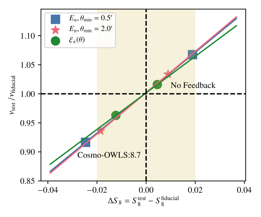
Figure 19: Estimating the expected bias $\Delta S_{8}$ when analysing a Universe with no baryon feedback (upper right quadrant) or a Universe with strong AGN feedback, modelled with Cosmo-OWLS:8.7 (lower left quadrant), with a fiducial theoretical model that adopts HMCode2020 with $\log_{10}(T_{\rm AGN}/{\rm K})=7.8$. We determine the signal-to-noise $\nu$ (Equation 136) for three mock cosmic shear observables: DES Y3 $\xi_{\pm}(\theta)$ including scale cuts (green), KiDS-1000 COSEBIs $E_{n}$ with $\theta_{\rm min}=$ 2$\stackrel{{\>{}^{\prime}}}{{\textstyle.}}$0 (pink) and KiDS-1000 $E_{n}$ with $\theta_{\rm min}=$ 0$\stackrel{{\>{}^{\prime}}}{{\textstyle.}}$5 (blue). This is calculated for the fiducial model over a range of $S_{8}$ values (solid lines), and also for the trial cases of no feedback, and strong feedback (data points). As expected the two scale cut statistics ($\xi_{\pm}(\theta)$ - circle, $E_{n},\theta_{\rm min}=$ 2$\stackrel{{\>{}^{\prime}}}{{\textstyle.}}$0 - star) produce the least biased estimate when the underlying feedback differs from the model. The offset between the two COSEBIs statistics is within the $1\sigma$ error for a KiDS-like analysis (shaded).

In the interest of conducting a fast approximate analysis, we choose to compress the tomographic cosmic shear data vector into a single signal-to-noise estimate $\nu$ (Equation 136), following Appendix E.1. By noting that the amplitude of the cosmic shear signal scales roughly as $\nu\propto S_{8}^{2}$ (Jain & Seljak, 1997), we can write that the ratio $\nu_{\rm A}/\nu_{\rm B}\propto\Delta S_{8}$, for the same noise realisation of cosmology A and B whose $S_{8}$ values differ by a small quantity $\Delta S_{8}=S_{8}^{\rm A}-S_{8}^{\rm B}$.

In Figure 19 we calibrate this relationship by calculating the ratio of $\nu_{\rm test}/\nu_{\rm fiducial}$ for a series of mock KiDS-1000 and DES Y3 data vectors, using test cosmologies that differ from our fiducial cosmological parameter set in Table 6 with $S_{8}^{\rm test}=S_{8}^{\rm fiducial}+\Delta S_{8}$. We find a slightly different relationship for the DES Y3-like $\xi_{\pm}(\theta)$ data vector (green) and the KiDS-1000-like $E_{n}$ data vectors (pink, blue), but a similar response for the two COSEBIs statistic versions with $\theta_{\rm min}=$ 0$\stackrel{{\>{}^{\prime}}}{{\textstyle.}}$5 (blue) and $\theta_{\rm min}=$ 2$\stackrel{{\>{}^{\prime}}}{{\textstyle.}}$0 (pink).

To address the question, what offset in $S_{8}$ would we expect to measure from the different cosmic shear statistics if our baryon feedback model was incorrect, we calculate $\nu_{\rm test}/\nu_{\rm fiducial}$ for two further tests. In both tests the cosmological model is fixed to the fiducial parameter set and the baryon feedback model is altered. First we adopt a dark matter only matter power spectrum with no baryon feedback suppression. The fiducial mock simulates baryon feedback with $\log_{10}(T_{\rm AGN}/{\rm K})=7.8$, reducing power relative to the dark matter only case by a factor of $\sim 5\%$ at $k=1h{\rm Mpc}^{-1}$. In this case $\nu_{\rm test}/\nu_{\rm fiducial}>1$ (see the upper right quadrant in Figure 19). For the second test we adopt a model from the most extreme baryon feedback simulation to date Cosmo-OWLS:8.7 (Le Brun et al., 2014), which reduces power relative to the dark matter only case by a factor of $\sim 20\%$ at $k=1h{\rm Mpc}^{-1}$, roughly a factor of four times the level of suppression relative to the fiducial $\log_{10}(T_{\rm AGN}/{\rm K})=7.8$ case. In this test $\nu_{\rm test}/\nu_{\rm fiducial}<1$ (see the lower left quadrant in Figure 19). Using the $\nu_{\rm A}/\nu_{\rm B}\propto\Delta S_{8}$ relationship calibrated for each statistic in Figure 19, we can read off an estimate for $\Delta S_{8}$ for these two test cases. As expected we find the COSEBIs $\theta_{\rm min}=$ 0$\stackrel{{\>{}^{\prime}}}{{\textstyle.}}$5 statistic (blue) to be the most sensitive to baryon feedback (the largest $\Delta S_{8}$ values), followed by COSEBIs $\theta_{\rm min}=$ 2$\stackrel{{\>{}^{\prime}}}{{\textstyle.}}$0 (pink) and then $\xi_{\pm}(\theta)$ with DES Y3 scale cuts applied. The difference seen between the COSEBIs $\theta_{\rm min}=$ 2$\stackrel{{\>{}^{\prime}}}{{\textstyle.}}$0 and $\xi_{\pm}(\theta)$ scale cut analyses demonstrates that the COSEBIs-defined scale cut from Appendix B renders the cosmic shear analysis more sensitive to the $k$-scales impacted by baryon feedback, compared to the Krause et al. (2021) $\xi_{\pm}(\theta)$-defined scale cuts. It may be beneficial in the future to develop the COSEBIs software to allow for redshift-dependent $\theta_{\rm min}$-limits in order to further reduce the impact of baryon feedback without incurring a significant loss of constraining power.

What is of interest for this appendix is the $S_{8}$ offset found between the different statistics, rather than the offset relative to the fiducial input value. If the underlying truth was a Universe with no baryon feedback, in a noise-free analysis we would expect our best fit value for $S_{8}$ to decrease by $\Delta S_{8}=0.012$ when changing from $\theta_{\rm min}=$ 0$\stackrel{{\>{}^{\prime}}}{{\textstyle.}}$5 to $\theta_{\rm min}=$ 2$\stackrel{{\>{}^{\prime}}}{{\textstyle.}}$0. This corresponds to a $\sim 0.6\sigma$ decrease between the different KiDS-1000 constraints. In the data we find a higher $S_{8}$ value when scale cuts are included, which is more similar to the case where the underlying truth is Cosmo-OWLS:8.7. Here we would expect to measure an increase of $\Delta S_{8}=0.008$ between the two noise-free COSEBIs analyses, corresponding to a $0.4\sigma$ offset between the different KiDS-1000 constraints.

It is important to recognise that these estimates are only approximate as they compress the tomographic data vector into a single noise-averaged value, erasing second-order information on scale and redshift dependence. In one respect, however, they are conservative, as they do not account for the marginalisation step over a wide baryon feedback prior in the KiDS-like analysis that allows for models as strong as $\log_{10}(T_{\rm AGN}/{\rm K})=8.0$. From this analysis we draw the conclusion that the $S_{8}$ offset we measure between the KiDS-1000 COSEBIs $\theta_{\rm min}=$ 0$\stackrel{{\>{}^{\prime}}}{{\textstyle.}}$5 and $\theta_{\rm min}=$ 2$\stackrel{{\>{}^{\prime}}}{{\textstyle.}}$0 $E_{n}$ constraints could be attributed to unmodeled extreme baryon feedback. This hypothesis only accounts for roughly half of the observed difference, however, when considering Cosmo-OWLS:8.7 as the ‘worst-case scenario’ for baryon feedback.

Asgari et al. (2021) report cosmological parameter constraints from a range of two-point statistics measured from the same data set: $E_{n}(\theta_{\rm min}=$0$\stackrel{{\>{}^{\prime}}}{{\textstyle.}}$5$)$, $\xi_{\pm}(\theta)$ and $C^{\rm EE}_{\epsilon\epsilon}(\ell)$. Using a series of 5000 noisy mock simulations of KiDS-1000 created with SALMO, they quantify the cross-correlation between the different statistics. The range of positive, zero and negative cross-correlations for different components result from the changing sensitivity of each statistic to a range of noisy $\ell$-scales. Asgari et al. (2021) find that they expect to measure a $>1\sigma$ offset in $S_{8}$ constraints between the different KiDS-1000 two-point statistics, 15% of the time (see similar findings for analyses of HSC-Y1 mocks in Hamana et al., 2022). The $0.3\sigma$ offset between the fiducial $\xi_{\pm}(\theta)$ and $E_{n}$ constraints seen in Table 13 is therefore expected.

We revisit the Asgari et al. (2021) analysis to quantify the expected offset in $S_{8}$ between two COSEBIs analyses of the same data set using $\theta_{\rm min}=$ 0$\stackrel{{\>{}^{\prime}}}{{\textstyle.}}$5 and $\theta_{\rm min}=$ 2$\stackrel{{\>{}^{\prime}}}{{\textstyle.}}$0. Using the original set of SALMO mocks, we were able to determine the cross-correlation between the two COSEBIs versions at essentially no CPU cost. We then took a short-cut compared to the original analysis, using the $\nu_{\rm A}/\nu_{\rm B}\propto\Delta S_{8}$ relationship derived in Figure 19 to determine the expected offset in $S_{8}$ between pairs of $E_{n}$ statistics measured with and without scale cuts in each SALMO mock. This differs from the CPU-intensive approach of Asgari et al. (2021) where full CosmoSIS analyses were performed for each mock and each statistic. By applying the same short-cut technique to the set of statistics tested in Asgari et al. (2021), however, we have verified that this approximate approach results in a similar distribution in $\Delta S_{8}$ values. We find that a $\geq 1\sigma$ offset in $S_{8}$ between the two COSEBIs measurements is expected 9% of the time. As such the two COSEBIs versions are more correlated with each other than with $\xi_{\pm}(\theta)$ and $C^{\rm EE}_{\epsilon\epsilon}(\ell)$. For the $0.7\sigma$ difference that we observe in the HMCode2016 analysis, we find that an offset of $\geq 0.7\sigma$ is expected 23% of the time. An offset of $\geq 0.8\sigma$ is expected 14% of the time. As such the offsets we find between the scale cut and original version of COSEBIs with KiDS-1000 can be attributed to random noise fluctuations.

To the reader most familiar with the $\xi_{\pm}(\theta)$ statistic, this result may seem counter-intuitive, as the scale cut that has been applied removes only one data point from each tomographic bin. As we can see in Table 13, a $\xi_{\pm}(\theta)$ analysis with a $\theta_{\rm min}=$ 2$\stackrel{{\>{}^{\prime}}}{{\textstyle.}}$0 scale cut applied indeeds makes little impact, with $S_{8}$ changing by $\sim 0.2\sigma$. In contrast, the COSEBIs statistic is calculated as a weighted average of finely binned noisy measurements of $\xi_{\pm}(\theta)$ summed over the range $\theta_{\rm min}<\theta<\theta_{\rm max}$. The shape of the oscillatory weight functions depends on the angular range limits (see equations 28 and 38 of Schneider et al., 2010). For $\theta_{\rm min}=$ 0$\stackrel{{\>{}^{\prime}}}{{\textstyle.}}$5 and $\theta_{\rm min}=$ 2$\stackrel{{\>{}^{\prime}}}{{\textstyle.}}$0 it is worth noting that the COSEBIs weight functions differ significantly for $\theta\lesssim$ 40$\stackrel{{\>{}^{\prime}}}{{\textstyle.}}$0.

Appendix G Constraints on all parameters, additional tables and figures

Summary: In this appendix we present additional results from the DES Y3 + KiDS-1000 cosmic shear analysis to complement the primary results in Section 3.

Survey	Pipeline	$\chi^{2}_{\rm min}$	$N_{\Theta}$	$p(\chi_{\rm min}^{2}|\nu_{\rm eff}$)
DES Y3 (Full area)	DES-like	283.6	6.7	0.222
DES Y3 (Full area)	KiDS-like	284.3	5.0	0.235
DES Y3 (Full area)	Hybrid	284.2	5.4	0.231
DES Y3 (KiDS-excised)	DES-like	285.3	8.0	0.187
DES Y3 (KiDS-excised)	KiDS-like	286.5	5.1	0.207
DES Y3 (KiDS-excised)	Hybrid	288.3	4.6	0.192
KiDS	DES-like	83.7	8.3	0.078
KiDS	KiDS-like	82.5	6.5	0.118
KiDS	Hybrid	88.3	7.1	0.048
Joint	DES-like	371.5	12.0	0.089
Joint	KiDS-like	381.3	7.8	0.062
Joint	Hybrid	378.0	9.6	0.068
Joint-1IA	DES-like	377.2	10.4	0.068
Joint-1IA	KiDS-like	373.9	8.8	0.094
Joint-1IA	Hybrid	382.2	8.0	0.057

Table 14: Goodness of fit statistics listing the $\chi^{2}_{\rm min}$, the effective number of parameters, $N_{\Theta}$, and the goodness of fit statistic $p(\chi^{2}>\chi^{2}_{\rm min}|\nu)$ (see Section 2.7 for details). The Hybrid pipeline results can be compared to the DES-like and KiDS-like analysis of DES, KiDS and the joint survey.

Parameter	DES Y3+KiDS-1000	DES Y3	KiDS-1000
$S_{8}$	$0.790^{+0.018}_{-0.014}$	$0.802^{+0.023}_{-0.019}$	$0.763^{+0.031}_{-0.023}$
$\Omega_{\rm m}$	$0.280^{+0.037}_{-0.046}$	$0.297^{+0.040}_{-0.060}$	$0.270^{+0.056}_{-0.102}*$
$\sigma_{8}$	$0.825^{+0.067}_{-0.073}$	$0.816^{+0.076}_{-0.085}$	$0.833^{+0.133}_{-0.146}$
$h$	$0.746^{+0.069}_{-0.029}*$	$0.738^{+0.072}_{-0.040}*$	$0.749^{+0.068}_{-0.029}*$
$n_{\rm s}$	$0.973^{+0.074}_{-0.072}*$	$0.979^{+0.093}_{-0.062}*$	$0.984^{+0.102}_{-0.053}*$
$\Sigma m_{\nu}$	$0.326^{+0.110}_{-0.187}*$	$0.317^{+0.139}_{-0.223}*$	$0.327^{+0.152}_{-0.215}*$
$\omega_{\rm b}$	$0.022^{+0.002}_{-0.003}*$	$0.022^{+0.002}_{-0.003}*$	$0.022^{+0.002}_{-0.003}*$
$\mathrm{log}_{10}(T_{\mathrm{AGN}}/{\rm K)}$	$7.627^{+0.152}_{-0.299}*$	$7.632^{+0.170}_{-0.289}*$	$7.623^{+0.153}_{-0.293}*$
$A_{\rm IA}^{\mathrm{DES}}$	$-0.025^{+0.576}_{-0.285}$	$0.323^{+0.432}_{-0.369}$	-
$\eta^{\mathrm{DES}}$	$2.047^{+2.953}_{-0.832}*$	$1.774^{+3.166}_{-0.940}*$	-
$A_{\rm IA}^{\mathrm{KiDS}}$	$1.038^{+0.543}_{-0.516}$	-	$0.650^{+0.884}_{-0.539}$
$\eta^{\mathrm{KiDS}}$	$2.211^{+2.588}_{-0.958}*$	-	$2.022^{+2.937}_{-0.868}*$
$\Delta z_{1}^{\mathrm{DES}}$	$0.001^{+0.015}_{-0.015}*$	$-0.004^{+0.016}_{-0.015}*$	-
$\Delta z_{2}^{\mathrm{DES}}$	$0.014^{+0.012}_{-0.011}*$	$0.011^{+0.011}_{-0.011}*$	-
$\Delta z_{3}^{\mathrm{DES}}$	$-0.008^{+0.010}_{-0.010}*$	$-0.004^{+0.010}_{-0.010}*$	-
$\Delta z_{4}^{\mathrm{DES}}$	$-0.006^{+0.015}_{-0.014}*$	$0.000^{+0.014}_{-0.014}*$	-
$\Delta z_{1}^{\mathrm{KiDS}}$	$-0.001^{+0.011}_{-0.010}*$	-	$0.000^{+0.010}_{-0.010}*$
$\Delta z_{2}^{\mathrm{KiDS}}$	$-0.010^{+0.010}_{-0.011}*$	-	$-0.008^{+0.011}_{-0.012}*$
$\Delta z_{3}^{\mathrm{KiDS}}$	$0.016^{+0.010}_{-0.011}*$	-	$0.016^{+0.011}_{-0.010}*$
$\Delta z_{4}^{\mathrm{KiDS}}$	$0.017^{+0.008}_{-0.009}*$	-	$0.015^{+0.008}_{-0.008}*$
$\Delta z_{5}^{\mathrm{KiDS}}$	$-0.006^{+0.009}_{-0.010}*$	-	$-0.007^{+0.009}_{-0.010}*$
$m_{1}^{\mathrm{DES}}$	$-0.007^{+0.009}_{-0.009}*$	$-0.007^{+0.009}_{-0.009}*$	-
$m_{2}^{\mathrm{DES}}$	$-0.021^{+0.008}_{-0.007}*$	$-0.020^{+0.008}_{-0.008}*$	-
$m_{3}^{\mathrm{DES}}$	$-0.022^{+0.007}_{-0.007}*$	$-0.024^{+0.007}_{-0.008}*$	-
$m_{4}^{\mathrm{DES}}$	$-0.035^{+0.007}_{-0.007}*$	$-0.037^{+0.007}_{-0.007}*$	-

Table 15: Mean marginal constraints with 68% credible intervals for the $\Lambda$CDM parameters (upper), astrophysical nuisance parameters (middle) and data calibration parameters (lower). Cosmic shear results are reported from the joint DES Y3 and KiDS-1000 (left), DES Y3 (middle) and KiDS-1000 (right) analyses. Parameters marked ^∗, are considered to be unconstrained by the data as their marginal posterior, at either prior edge, exceeds 13% of the peak posterior probability.

• Table 14 presents the goodness of fit statistics for the DES-like and KiDS-like analyses, listing the $\chi^{2}_{\rm min}$, the estimated effective number of parameters, $N_{\Theta}$, and the goodness of fit statistic $p(\chi^{2}>\chi^{2}_{\rm min}|\nu)$ for a range of different analyses of the DES, KiDS and joint-survey data vectors, with $N_{\rm data}=273,75,348$ respectively. We remind the reader that the Joachimi et al. (2021) approach used to estimate $N_{\Theta}$ is subject to noise at the level of $\sim 0.2N_{\Theta}$.

• In Figure 20 we present the joint-survey constraints across the full cosmological parameter space, comparing the fiducial Hybrid NLA-z analysis with the alternative TATT analysis. We also include the marginal posterior for the baryon feedback parameter $T_{\rm AGN}$. Only $S_{8}$, $\Omega_{\rm m}$ and $\sigma_{8}$ are constrained by the data. The axis limits on $h,n_{\rm s},\Sigma m_{\nu}$, $\omega_{\rm b}$ and $T_{\rm AGN}$ are set by the priors. As we have chosen to sample in $S_{8}$, the prior space is straightforward to visualise as rectangles in each 2D marginal bounded by the prior edges. Throughout the paper we use GetDist (Lewis, 2019) to plot quantities of interest from our chains of Monte Carlo samples. GetDist applies a linear boundary kernel and multiplicative bias correction to remove the bias introduced when the chain-smoothing kernel passes over a prior boundary. When the hard boundaries from the priors are aligned with the parameter coordinates, as in our case, the boundaries can be defined using the GetDist.MCSamples ‘ranges’ option. With the prior ranges set, the GetDist contoured credible intervals do not artificially close for prior-informed parameters.

• In Figure 21 we present the joint-survey constraints across the astrophysical nuisance parameter space for the alternative TATT analysis. Only $S_{8}$, $a_{1}$ and $a_{2}$ are constrained by the data. We can see that the preference for a lower $S_{8}$ value in the TATT analysis, relative to our fiducial analysis, is primarily driven by the IA model allowing for a significant tidal torque amplitude, the $a_{2}$ parameter, when there is strong redshift evolution with high values for $\eta_{2}$. We find a similar preference for strong redshift evolution of the IA model in the fiducial NLA-z analysis (see Figure 3), but in contrast to the TATT analysis, the $\eta_{\rm IA}$ amplitude is largely uncorrelated with $S_{8}$. We see similar behaviour for the IA model parameters for the DES (pink) and KiDS (black) surveys. As with the fiducial analysis, KiDS prefers higher values for $A_{1}$ compared to DES.

• Table 15 reports the mean 1D marginal values for each parameter for the fiducial Hybrid analyses of DES Y3 and KiDS-1000. We use ^∗ to mark parameters that are unconstrained by the data. In these cases the tabulated constraint comes from the prior, as the marginal posterior probability, at either prior edge, exceeds 13% of the peak posterior value (see appendix A of Asgari et al., 2021). We constrain $S_{8}$, $\sigma_{8}$, and the intrinsic alignment amplitude $A_{\rm IA}$ for each survey, and $\Omega_{\rm m}$ for the joint survey and the DES-only analysis. We have not presented figures of the marginal posteriors for the shear and redshift calibration nuisance parameters $m$ and $\Delta z$, as we recover the peak and width of the Gaussian prior for the majority of these parameters (compare the values in Table 1 and Table 15). A notable exception is the redshift calibration parameter for the second tomographic bin, $\Delta z_{2}$, for both the DES and KiDS data. In the DES-only, KiDS-only and joint-survey Hybrid analysis the mean $\Delta z_{2}$ of each survey is $\pm 1\sigma$ offset from the Gaussian prior peak. This is consistent with the previous findings of both survey teams (see for example figure 17 of Amon et al., 2022). Both teams show consistent $S_{8}$ results when excluding individual tomographic bins from the fiducial analysis (see also figures 16 and 18 in Amon et al., 2022, for the stability of the intrinsic alignment parameter constraints when removing redshift bins and varying the redshift calibration methodology). Using the Köhlinger et al. (2019) ‘three tier’ set of internal consistency statistics, Asgari et al. (2021) flag the second KiDS-1000 tomographic bin as an outlier (see their appendix B.2). As this bin carries insignificant levels of cosmological information, however, the results are unchanged by the inclusion or exclusion of this tomographic bin.

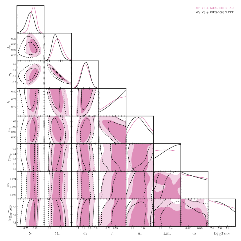
Figure 20: Joint survey posteriors for the $\Lambda$CDM cosmological parameters and the HMCode2020 $T_{\rm AGN}$ parameter for baryonic feedback. We compare the fiducial Hybrid (NLA-z) analysis in pink to a TATT analysis with black dashed lines. The inner 68% and outer 95% credible intervals are shown contoured. In the case of the parameters $h,n_{\rm s},\Sigma m_{\nu}$, $\omega_{\rm b}$ and $T_{\rm AGN}$, the axis limits are set by the prior boundaries.

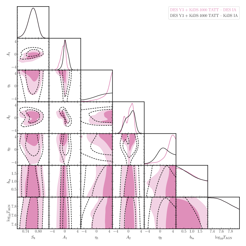
Figure 21: Joint survey posteriors, comparing constraints on the TATT intrinsic alignment model (see Section 2.2) from the DES Y3 (pink) and KiDS-1000 (black-dashed) surveys with the inner 68% and outer 95% credible intervals contoured. In all but the $S_{8}$ parameter, the axis limits are set by the prior boundaries.

References

- Abdalla et al. (2022) Abdalla E., et al., 2022, Journal of High Energy Astrophysics, 34, 49
- Adamek et al. (2023) Adamek J., et al., 2023, J. Cosmology Astropart. Phys, 2023, 035
- Aihara et al. (2018) Aihara H., et al., 2018, PASJ, 70, S4
- Amodeo et al. (2021) Amodeo S., et al., 2021, Phys. Rev. D, 103, 063514
- Amon & Efstathiou (2022) Amon A., Efstathiou G., 2022, MNRAS, 516, 5355
- Amon et al. (2018) Amon A., et al., 2018, MNRAS, 477, 4285
- Amon et al. (2022) Amon A., et al., 2022, Phys. Rev. D, 105, 023514
- Amon et al. (2023) Amon A., Robertson et al., 2023, MNRAS, 518, 477
- Andrade-Oliveira et al. (2021) Andrade-Oliveira F., et al., 2021, MNRAS, 505, 5714
- Aricò et al. (2023) Aricò G., Angulo R. E., Zennaro M., Contreras S., Chen A., Hernández-Monteagudo C., 2023, A&A, 678, A109
- Asgari et al. (2019) Asgari M., et al., 2019, A&A, 624, A134
- Asgari et al. (2020) Asgari M., Tröster T., et al., 2020, A&A, 634, A127
- Asgari et al. (2021) Asgari M., et al., 2021, A&A, 645, A104
- Asgari et al. (2023) Asgari M., Mead A. J., Heymans C., 2023, arXiv e-prints, arXiv:2303.08752
- Bacon et al. (2000) Bacon D. J., Refregier A. R., Ellis R. S., 2000, MNRAS, 318, 625
- Bartelmann & Schneider (2001) Bartelmann M., Schneider P., 2001, Phys. Rep., 340, 291
- Benítez (2000) Benítez N., 2000, ApJ, 536, 571
- Benitez et al. (2014) Benitez N., et al., 2014, arXiv e-prints, arXiv:1403.5237
- Benjamin et al. (2007) Benjamin J., et al., 2007, MNRAS, 381, 702
- Beran (1977) Beran R., 1977, The Annals of Statistics, 5, 445
- Bianchini et al. (2020) Bianchini F., et al., 2020, ApJ, 888, 119
- Bird et al. (2012) Bird S., Viel M., Haehnelt M. G., 2012, MNRAS, 420, 2551
- Blazek et al. (2019) Blazek J. A., MacCrann N., Troxel M. A., Fang X., 2019, Phys. Rev. D, 100, 103506
- Bridle & King (2007) Bridle S., King L., 2007, New Journal of Physics, 9, 444
- Buchs et al. (2019) Buchs R., et al., 2019, MNRAS, 489, 820
- Campos et al. (2023) Campos A., Samuroff S., Mandelbaum R., 2023, MNRAS, 525, 1885
- Capozzi et al. (2016) Capozzi F., Lisi E., Marrone A., Montanino D., Palazzo A., 2016, Nuclear Physics B, 908, 218
- Chang et al. (2019) Chang C., et al., 2019, MNRAS, 482, 3696
- Chen et al. (2023) Chen A., et al., 2023, MNRAS, 518, 5340
- Chiang et al. (2020) Chiang Y.-K., Makiya R., Ménard B., Komatsu E., 2020, ApJ, 902, 56