2 mm Observations and the Search for High-Redshift Dusty Star-forming Galaxies

Abstract

Finding high-redshift ($z\gg 4$) dusty star-forming galaxies is extremely challenging. It has recently been suggested that millimeter selections may be the best approach, since the negative K-correction makes galaxies at a given far-infrared (FIR) luminosity brighter at $z\gtrsim 4$ than those at $z=2$–3. Here we analyze this issue using a deep ALMA 2 mm sample obtained by targeting ALMA 870 $\mu$m priors (these priors were the result of targeting SCUBA-2 850 $\mu$m sources) in the GOODS-S. We construct prior-based 2 mm galaxy number counts and compare them with published blank field-based 2 mm counts, finding good agreement down to 0.2 mJy. Only a fraction of the current 2 mm extragalactic background light is resolved, and we estimate what observational depths may be needed to resolve it fully. By complementing the 2 mm ALMA data with a deep SCUBA-2 450 $\mu$m sample, we exploit the steep gradient with redshift of the 2 mm to 450 $\mu$m flux density ratio to estimate redshifts for those galaxies without spectroscopic or robust optical/near-infrared photometric redshifts. Our observations measure galaxies with star formation rates in excess of 250 M_⊙ yr^-1. For these galaxies, the star formation rate densities fall by a factor of 9 from $z=2$–3 to $z=5$–6.

1 Introduction

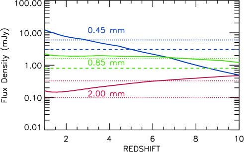
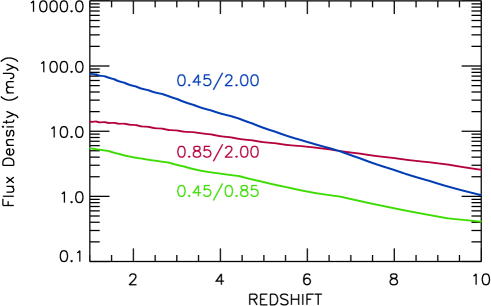
Figure 1: (a) Flux vs. redshift curves (solid) for a source with $L_{\rm FIR}=10^{12}$ L_⊙ at 450 $\mu$m (blue), 850 $\mu$m (green), and 2 mm (red), using Arp 220 as a template for the SED shape (Silva et al., 1998). The 450 $\mu$m flux has the steepest gradient and hence is critical for identifying high-redshift candidates. From top to bottom, the $4\sigma$ flux limits are 6 mJy at 450 $\mu$m for SCUBA-2 blank fields (Barger et al., 2022) (blue dotted) and a factor of 2 deeper for SCUBA-2 lensing cluster fields (Cowie et al., 2022) (blue dashed), assuming a factor of 2 magnification typical of the fainter sources in Cowie et al. (2022); the 1.65 mJy confusion limit at 850 $\mu$m for SCUBA-2 blank fields (Cowie et al., 2017) (green dotted) and again a factor of 2 deeper for SCUBA-2 lensing cluster fields (green dashed); 0.33 mJy for the ALMA MORA 2 mm survey (Casey et al., 2021) (red dotted); and 0.13 mJy for the ALMACAL 2 mm survey (Chen et al., 2023) (red dotted). (b) Flux ratio vs. redshift curves for $f_{450\,\mu{\rm m}}/f_{2\,{\rm mm}}$ (blue), $f_{850\,\mu{\rm m}}/f_{2\,{\rm mm}}$ (red), and $f_{450\,\mu{\rm m}}/f_{850\,\mu{\rm m}}$ (green).

The discovery of the far-infrared (FIR) extragalactic background light (EBL) by COBE demonstrated that about half of the universe’s starlight at UV/optical wavelengths is absorbed by dust and reradiated into the FIR (Puget et al., 1996; Fixsen et al., 1998). Moreover, from individual source measurements in the $z$ = 1–4 redshift range, it has been found that up to five times as much starlight is radiated into the FIR as is seen in the UV/optical (e.g., Wang et al., 2006; Zavala et al., 2021). We therefore need to study both the unobscured and dust-obscured populations of galaxies across cosmic time to obtain a complete picture of the star formation in our universe. However, even multiwavelength galaxy number counts alone—the projected galaxy surface density with flux—can provide critical constraints on galaxy modeling and help us to understand the physical processes behind galaxy formation and evolution (e.g., Shimizu et al., 2012; Schaye et al., 2015; Davé et al., 2019; Lagos et al., 2020; Popping et al., 2020).

The galaxy number counts are now well established at both 450 $\mu$m and 850 $\mu$m (e.g., Chen et al., 2013; Hsu et al., 2016; Wang et al., 2017; Zavala et al., 2017; Béthermin et al., 2020; Barger et al., 2022). Although there have been efforts to measure the 2 mm number counts with GISMO (Staguhn et al., 2014; Magnelli et al., 2019) on the Institute for Radioastronomy at Millimeter Wavelengths (IRAM) 30 m telescope and with the Atacama Large Millimeter/submillimeter Array (ALMA) (Zavala et al., 2021; Chen et al., 2023), these map only a fraction of the EBL. With NIKA2 (Adam et al., 2018) now on IRAM and the commissioning of TolTEC (Wilson et al., 2020) on the Large Millimeter Telescope 50 m, which has a higher resolution (at 2 mm, TolTEC’s resolution is $9\farcs 5$ versus NIKA2’s $17\farcs 5$), it is of interest to determine how deep of observations will be needed to measure the full EBL at 2 mm.

Despite several decades of work, determining the number of dusty star-forming galaxies (DSFGs) at high redshifts continues to be a major challenge, since high-redshift DSFGs are often too faint for optical/near-infrared (NIR) spectroscopic redshifts (e.g., Cowie et al., 2009; Wang et al., 2009; Barger et al., 2014; Dudzevičiūtė et al., 2020; Smail et al., 2021). It has been suggested (e.g., Casey et al., 2021) that observations at 2 mm might provide a promising means for finding such galaxies, since for a given FIR luminosity, the negative K-correction makes galaxies at $z\gtrsim 4$ slightly brighter at 2 mm than those at $z\sim 2$–3 (see Figure 1(a)); however, the curve is quite flat. By comparison, the 850 $\mu$m flux drops by these higher redshifts. Then, through the use of the 2 mm to 870 $\mu$m flux ratio, one can try to estimate redshifts for these galaxies (e.g., Casey et al., 2021; Cooper et al., 2022). However, as we discuss in this paper, redshifts are better estimated using the flux ratio of 2 mm to a shorter bandpass, such as 450 $\mu$m, where the gradient is steeper (see Figure 1(b)). Thus, observations at shorter wavelengths are critical for separating high-redshift candidates from lower redshift sources.

DSFGs are sparse (e.g., $\sim 1$ source per 1 arcmin² at an 850 $\mu$m flux of 2 mJy; Hsu et al. 2016), so it is very inefficient to map them with small field-of-view instruments, though the ALMA sensitivity is such that modest samples can be generated with enough invested time (e.g., Dunlop et al., 2017; González-López et al., 2017; Franco et al., 2018; Hatsukade et al., 2018; Aravena et al., 2020; Casey et al., 2021; Gómez-Guijarro et al., 2022). Instead, the best method to select high-redshift DSFGs systematically remains submillimeter/millimeter surveys from large-aperture, ground-based telescopes, as these provide the fields-of-view necessary to detect significant samples. These samples can then be efficiently followed up with interferometric observations (e.g., Barger et al., 2012; Hodge et al., 2013; Cowie et al., 2017, 2018, 2022; Stach et al., 2019; Cooper et al., 2022). In fact, using single-dish priors can provide an enormous gain in speed over direct interferometric searches. At 2 mJy, there are about 3000 850 $\mu$m sources per 1 deg² (e.g., Hsu et al., 2016). This is the number of targeted ALMA pointings one would need to image this population. In contrast, given the ALMA $16\farcs 9$ FWHM at this wavelength, one would need about 57000 ALMA pointings to image fully this area at the same level. Thus, targeted ALMA imaging gives a speed gain of a factor of roughly 19 over ALMA mosaicking.

In this paper, we present new ALMA 2 mm observations of the ALMA 870 $\mu$m GOODS-S sample from Cowie et al. (2018), which was based on ALMA follow-up of the confusion-limited SCUBA-2 850 $\mu$m observations of the field. We construct the 2 mm cumulative number counts, which we compare with the literature, and we estimate how deep of 2 mm observations are needed to fully resolve the EBL at this wavelength. In combination with new deep SCUBA-2 450 $\mu$m observations of the field, we demonstrate the advantages of using the 2 mm to 450 $\mu$m flux ratio for identifying candidate high-redshift DSFGs.

In Section 2, we describe our new ALMA 2 mm and SCUBA-2 450 $\mu$m observations and data reduction. In Section 3, we examine the dependence of the 2 mm to 870 $\mu$m flux density ratio on the 870 $\mu$m flux density. In Section 4, we construct 2 mm cumulative and differential number counts, which we compare with the literature. In Section 5, we consider three flux density ratios, $f_{450\,\mu{\rm m}}/f_{2\,{\rm mm}}$, $f_{870\,\mu{\rm m}}/f_{2\,{\rm mm}}$, and $f_{450\,\mu{\rm m}}/f_{870\,\mu{\rm m}}$, for identifying candidate high-redshift DSFGs. We then estimate the star formation history. In Section 6, we summarize our results.

We assume $\Omega_{M}=0.3$, $\Omega_{\Lambda}=0.7$, and $H_{0}=70$ km s^-1 Mpc^-1 throughout.

Figure 2: Median ratio of the aperture flux to the peak flux vs. the aperture radius for the 37 ALMA sources with 2 mm peak flux densities $>0.1$ mJy. The error bars show the 68% confidence range on the median.

2 Data

2.1 ALMA Observations

Cowie et al. (2018) provided a catalog of $>4\sigma$ sources from a SCUBA-2 850 $\mu$m survey of the GOODS-S. They also presented the 75 870 $\mu$m ALMA sources ($>4.5\sigma$) (their Table 4) that resulted from high-resolution interferometric follow-up observations of this sample. In ALMA program #2021.1.00024.S (PI: F. Bauer), we made ALMA spectral linescans in band 6 (central wavelength of 1.24 mm), band 4 (1.98 mm; hereafter, 2 mm), and band 3 (3.07 mm) of 57 sources in this sample. We focused on those sources with 870 $\mu$m flux densities above 1.8 mJy and without a very well-determined spectroscopic redshift, since spectroscopic redshifts were the primary goal of the observations.

In McKay et al. (2023), we presented the full ALMA data set (their Table 1) and fit the FIR spectral energy distributions (SEDs) of the sources to constrain the emissivity spectral indices and effective dust temperatures. Here we focus on the band 4 data, since there has been relatively little analysis of 2 mm number counts and faint 2 mm source properties in the literature.

In Table 1, we give our ALMA 2 mm flux densities in a table of Cowie et al. (2018)’s 75 sources to show which of the sources we observed. Of the 50 sources with 870 $\mu$m flux densities above 1.8 mJy and lying within a radial offset of $5\farcm 65$ from the SCUBA-2 image center (mean aim-point in J2000.0 coordinates: R.A. $03$:32:26.49, decl. $-27$:48:29.0), there are only 5 sources that we did not observe in band 4 (4 because they already had good spectroscopic redshifts; the fifth was inadvertently omitted).

The ALMA data were downloaded and calibrated using casa version 6.2.1-7 and PI scripts provided by ALMA. We visually inspected various diagnostic plots associated with the calibration to confirm that there were no unusual problems with particular antennas or baselines. The visibilities from individual spectral setups across each band were aggregated using concat, and dirty continuum images were generated using tclean, adopting 0$\farcs$25 pixels, natural weighting, and a “common” restoring beam. Based on the rms noise from the dirty images, cleaned continuum images were generated by adopting multi-threshold auto-masking with default values, assuming 10000 clean iterations, a flux threshold set to 3 times the rms ($\approx$0.06 mJy), pixel scales of 0, 5, and 10, and robust=0.5. As none of our targets are particularly bright, the dirty and clean images are nearly identical in terms of peak flux densities, noise, etc. We visually inspected the image products, confirming that there were no unusual noise residuals or patterns in the images. The resulting band 4 images had a central frequency of 151.188 GHz, a bandwidth of 23.375 GHz, and a beam of $\theta_{\rm beam}{=}$ 1$\farcs$21$\times$ 1$\farcs$10.

We additionally generated full-band spectral cubes with the same tclean parameters, adopting a native resolution of 16 MHz.

The peak flux densities, even in the tapered images, slightly underestimate the total flux densities (e.g., Cowie et al., 2018). The reason for this is that the sources are resolved. There are two methods we can use to estimate the total flux densities: We can take the ratio of the aperture measurements made in a range of aperture radii to the peak measurements, or we can fit the sources in the uv plane (e.g., Béthermin et al., 2020). Both give similar corrections (Cowie et al., 2018), and here we adopt the simpler aperture method. Because the aperture fits are noisy, we use a single average correction for all the sources. As we show in Figure 2, the median multiplicative correction asymptotes beyond an aperture radius of $\approx 1\farcs 5$, and we adopt this as our preferred radius, giving a multiplicative correction of 1.3.

Table 1: Flux and Redshift Table

C18			R.A.	decl.	Total		Peak		Peak
No.	Redshift	Ref.			$f_{870\,\mu{\rm m}}$	Error	$f_{450\,\mu{\rm m}}$	Error	$f_{2\,{\rm mm}}$	Error
			(J2000)	(J2000)	(mJy)		(mJy)		(mJy)
(1)	(2)	(3)	(4)	(5)	(6)	(7)	(8)	(9)	(10)	(11)
1	2.574	10	53.030373	-27.855804	8.93	0.21	22.99	3.46	0.61	0.02
2	3.690	10	53.047211	-27.870001	8.83	0.26	14.88	3.26	0.54	0.02
3	2.648	10	53.063877	-27.843779	6.61	0.16	18.68	2.46	0.33	0.02
4	2.252	4	53.020374	-27.779917	6.45	0.41	25.81	3.39	0.27	0.04
5	2.309	7	53.118790	-27.782888	6.39	0.16	13.67	1.87	0.26	0.03
6	$\cdots$	$\cdots$	53.195126	-27.855804	5.90	0.18	13.96	3.37	0.41	0.03
7	3.672	10	53.158371	-27.733612	5.60	0.14	5.49	2.78	0.38	0.02
8	2.69 (2.62–2.73)	0	53.105247	-27.875195	5.18	0.22	16.54	2.76	0.25	0.02
9	2.322	10	53.148876	-27.821167	5.09	0.12	17.27	2.21	0.32	0.04
10	2.41 (2.34–2.46)	0	53.082085	-27.767279	4.90	0.29	17.39	2.27	0.26	0.02
11	$\cdots$	$\cdots$	53.079376	-27.870806	4.76	0.29	14.21	2.79	0.28	0.02
12	3.764	1	53.142792	-27.827888	4.73	0.16	13.09	2.17	0.00	0.00
13	[2.73 (2.68–4.43)]	0	53.074837	-27.875916	4.69	0.81	7.04	2.84	0.33	0.02
14	2.73 (2.63–2.80)	0	53.092335	-27.826834	4.64	0.17	17.19	1.86	0.18	0.02
15	2.14 (2.06–2.23)	0	53.024292	-27.805695	3.93	0.15	11.70	3.23	0.17	0.02
16	3.37 (3.17–3.41)	0	53.082752	-27.866585	4.31	0.15	9.10	2.78	0.28	0.03
17	3.57 (3.45–3.81)	0	53.146629	-27.871029	3.80	0.18	9.26	2.56	0.21	0.02
18	3.847	8	53.092834	-27.801332	5.21	0.32	12.66	1.78	0.23	0.02
19	[4.47 (4.07–5.65)]	0	53.108795	-27.869028	3.62	0.17	7.34	2.80	0.24	0.02
20	1.93 (1.89–1.96)	0	53.198292	-27.747889	3.61	0.30	8.46	3.68	0.16	0.02
21	3.78 (3.70–3.83)	0	53.178333	-27.870222	3.55	0.20	8.90	3.09	0.18	0.02
22	2.698	9	53.183460	-27.776638	3.38	0.32	12.05	2.46	0.00	0.00
23	1.58 (1.56–1.61)	0	53.157207	-27.833500	3.32	0.29	8.58	2.42	0.14	0.02
24	1.96 (1.90–1.99)	0	53.102791	-27.892860	3.25	0.14	8.65	2.87	0.18	0.02
25	2.696	9	53.181377	-27.777557	3.18	0.23	9.41	2.42	0.00	0.00
26	3.78 (3.70–3.82)	0	53.070251	-27.845612	3.15	0.25	3.06	2.46	0.19	0.02
27	[1.78 (1.67–2.73)]	0	53.014584	-27.844389	3.05	0.19	9.49	4.43	0.16	0.03
28	[3.33 (3.20–4.38)]	0	53.139290	-27.890722	2.89	0.37	4.63	2.89	0.13	0.02
29	$\cdots$	$\cdots$	53.137127	-27.761389	2.82	0.28	15.27	2.41	0.13	0.02
30	1.86 (1.81–1.92)	0	53.071709	-27.843693	2.78	0.15	5.55	2.43	0.09	0.02
31	1.95 (1.89–2.00)	0	53.077377	-27.859612	2.54	0.43	7.04	2.70	0.07	0.02
32	2.75 (2.57–2.78)	0	53.049751	-27.770971	2.56	0.16	9.65	2.68	0.12	0.02
33	1.58 (1.53–1.61)	0	53.072708	-27.834278	2.49	0.23	12.96	2.27	0.08	0.03
34	1.95 (1.86–1.97)	0	53.090752	-27.782473	2.47	0.21	4.50	2.01	0.01	0.03
35	1.612	7	53.091747	-27.712166	2.47	0.13	12.53	3.32	0.10	0.02
36	2.37 (2.28–2.42)	0	53.086586	-27.810249	2.41	0.25	8.90	1.84	0.04	0.02
37	2.96 (2.87–3.05)	0	53.146378	-27.888807	2.35	0.28	4.36	2.92	0.10	0.03
38	2.31 (2.26–2.38)	0	53.092335	-27.803223	2.50	0.10	7.60	1.77	0.12	0.02
39	3.04 (2.99–3.21)	0	53.124332	-27.882696	2.26	0.18	10.42	2.71	0.04	0.03
40	2.224	3	53.131123	-27.773195	2.26	0.17	10.09	2.17	0.12	0.03
41	[4.13 (3.45–4.46)]	0	53.172832	-27.858860	2.25	0.18	1.99	2.65	0.17	0.02
42	2.34 (2.30–2.42)	0	53.091629	-27.853390	2.25	0.18	11.34	2.64	0.12	0.03
43	2.39 (2.32–2.62)	0	53.068874	-27.879723	2.23	0.41	14.33	3.03	0.16	0.03
44	$\cdots$	$\cdots$	53.087166	-27.840195	2.21	0.12	10.59	2.22	0.18	0.03
45	[7.62 (7.15–7.93)]	0	53.041084	-27.837721	2.43	0.21	7.25	2.80	0.14	0.02
46	1.613	1	53.104912	-27.705305	2.29	0.11	4.93	3.74	0.00	0.00
47	2.19 (2.12–2.22)	0	53.163540	-27.890556	2.05	0.15	1.06	3.65	0.07	0.02
48	2.543	6	53.160664	-27.776251	2.04	0.36	16.44	2.18	0.00	0.00
49	1.87 (1.84–1.93)	0	53.053669	-27.869278	1.98	0.23	10.56	3.08	0.07	0.03
50	1.69 (1.64–1.70)	0	53.089542	-27.711666	1.97	0.45	9.90	3.44	0.07	0.03
51	2.32 (2.29–2.43)	0	53.067833	-27.728889	1.94	0.22	8.00	2.95	0.10	0.02
52	[4.78 (4.35–5.10)]	0	53.064793	-27.862638	1.88	0.24	0.99	2.73	0.14	0.03
53	1.56 (1.50–1.60)	0	53.198875	-27.843945	1.86	0.32	7.09	3.23	0.00	0.00
54	[9.42 (9.35–9.83)]	0	53.181995	-27.814196	1.82	0.30	6.84	2.69	0.06	0.02
55	$\cdots$	$\cdots$	53.048378	-27.770306	1.79	0.15	6.42	2.74	0.06	0.02
56	2.299	3	53.107044	-27.718334	1.61	0.25	5.58	2.75	0.10	0.03
57	3.08 (3.00–3.68)	0	53.033127	-27.816778	1.72	0.26	0.48	2.98	0.00	0.00
58	[4.73 (4.39–4.90)]	0	53.183666	-27.836500	1.72	0.31	-1.2	2.74	0.19	0.03
59	2.325	3	53.094044	-27.804195	1.84	0.13	3.58	1.75	0.07	0.03
60	2.53 (2.41–2.60)	0	53.124584	-27.893305	1.61	0.25	6.81	2.88	0.00	0.00
61	[4.67 (4.48–5.23)]	0	53.132751	-27.720278	1.61	0.25	1.89	2.75	0.00	0.00
62	2.94 (2.88–3.03)	0	53.080669	-27.720861	1.59	0.17	8.08	3.11	0.00	0.00
63	1.83 (1.78–1.88)	0	53.120041	-27.808277	1.57	0.26	9.77	1.68	0.00	0.00
64	3.26 (3.20–3.40)	0	53.117085	-27.874918	1.53	0.31	6.84	2.72	0.00	0.00
65	1.58 (1.56–1.62)	0	53.131458	-27.841389	1.46	0.14	10.13	2.24	0.00	0.00
66	0.653	1	53.044708	-27.802027	1.44	0.26	5.20	2.92	0.00	0.00
67	1.69 (1.66–1.84)	0	53.072002	-27.819000	1.36	0.19	5.45	2.16	0.00	0.00
68	5.58	11	53.120461	-27.742083	1.35	0.24	3.46	2.53	0.00	0.00
69	2.55 (2.47–2.64)	0	53.113125	-27.886639	1.25	0.27	7.41	2.76	0.00	0.00
70	3.14 (3.06–3.34)	0	53.141251	-27.872860	1.18	0.25	8.21	2.61	0.04	0.02
71	1.71 (1.63–1.72)	0	53.056873	-27.798389	1.16	0.30	6.32	2.70	0.00	0.00
72	[3.76 (3.47–4.31)]	0	53.119957	-27.743137	1.11	0.29	-0.3	2.54	0.00	0.00
73	2.19 (2.09–2.22)	0	53.142872	-27.874084	1.07	0.17	8.15	2.61	0.01	0.02
74	0.732	1	53.093666	-27.826445	0.93	0.23	5.81	1.86	0.04	0.03
75	$\cdots$	$\cdots$	53.074837	-27.787111	0.84	0.14	3.49	2.25	0.00	0.00

Note. — The columns are (1) ALMA number from Cowie et al. (2018), (2) redshift (three digits after the decimal point for spectroscopic redshifts—except for the JWST NIRSpec redshift for source 68 from Oesch et al. (2023)—and two digits after the decimal point for photometric redshifts, plus 68% confidence ranges from Straatman et al. 2016 for photometric redshifts given in parentheses), (3) reference for redshift (see details below), (4) and (5) total ALMA 870 $\mu$m flux and error from Cowie et al. (2018), (6) and (7) measured peak SCUBA-2 450 $\mu$m flux and error from this work, and (8) and (9) measured peak ALMA 2 mm flux and error from this work. In Column (3), ‘0’ indicates a photometric redshift from Straatman et al. (2016) (poor quality flag $Q>3$ estimates are in square brackets to distinguish them from the more reliable $Q<3$ estimates), while all other numbers are spectroscopic redshifts: ‘1’ indicates the redshift is from our own Keck DEIMOS observations, ‘2’ is from K20 (Mignoli et al., 2005), ‘3’ is from MOSDEF (Kriek et al., 2015), ‘4’ is from Casey et al. (2011), ‘5’ is from Szokoly et al. (2004), ‘6’ is from Inami et al. (2017), ‘7’ is from Kurk et al. (2013), ‘8’ is from Franco et al. (2018) (B. Mobasher 2018, priv. comm.), ‘9’ is a CO redshift from González-López et al. (2019), ‘10’ is a CO redshift from Table 2, and ‘11’ is a JWST NIRSpec redshift from Oesch et al. (2023).

2.2 Redshifts

There are now spectroscopic redshifts for 20 sources (see Table 1). Most of these were listed in Table 5 of Cowie et al. (2018), but there are five new redshifts from the present ALMA linescans (see F. Bauer et al. 2023, in preparation). We summarize these in Table 2, along with the molecular lines that were used to determine them. Two others come from the ALMA SPECtroscopic Survey in the Hubble Ultra Deep Field (ASPECS; González-López et al., 2019). A final new redshift is from the JWST NIRSpec survey First Reionization Epoch Spectroscopically Complete Observations (FRESCO; Oesch et al. 2023).

In Table 1, we also provide photometric redshifts and their 68% confidence ranges from Straatman et al. (2016), who used the Easy and Accurate Zphot from Yale (EAZY) code (Brammer et al., 2008) to fit the FourStar Galaxy Evolution Survey (ZFOURGE) catalog from 0.3 to 8 $\mu$m. We note that some of these are tagged with a poor quality flag from EAZY, reflecting the unusual SEDs of these high-redshift DSFGs and the limited number of band detections. Following Cowie et al. (2018), we indicate the 11 sources with poor quality flag $Q>3$ estimates by putting their photometric redshifts in square brackets.

Table 2: ALMA Redshifts

No.	$z$	Line	Obs. Freq.	Redshift
			(GHz)
(1)	(2)	(3)	(4)	(5)
1	2.5740
		12CO($3\rightarrow 2$)	96.763	2.574
		12CO($5\rightarrow 4$)	161.223	2.574
		12CO($5\rightarrow 4$)	161.516	2.568
		12CO($5\rightarrow 4$)	159.883	2.604?
		12CO($5\rightarrow 4$)	161.399	2.570
2	3.694
		12CO($4\rightarrow 3$)	98.181	3.696
		12CO($6\rightarrow 5$)	147.300	3.694
		12CO($6\rightarrow 5$)	147.476	3.689
		H2O($2_{1,1}\rightarrow 2_{0,2})$	160.243	3.693
3	2.648
		12CO($3\rightarrow 2$)	94.778	2.648
		12CO($5\rightarrow 4$)	157.977	2.648
		12CO($5\rightarrow 4$)	157.856	2.651
7	3.672
		12CO($4\rightarrow 3$)	98.681	3.672
		12CO($6\rightarrow 5$)	148.019	3.672
		12CO($6\rightarrow 5$)	147.980	3.673
9	2.322
		[CI]($1\rightarrow 0$)	148.006	2.325
		HCO${}^{+}(6\rightarrow 5$)	161.187	2.320

Note. — The columns are (1) source number, (2) adopted redshift, (3) molecular line, (4) observed frequency, and (5) redshift obtained from each molecular line.

2.3 SCUBA-2 450 $\mu$m Observations

We have been obtaining SCUBA-2 observations of the GOODS-S for a number of years (see Cowie et al. 2018 and Barger et al. 2022 for recent analyses). Our primary goal is to obtain the deepest possible 450 $\mu$m observations. In order to maximize the depth in the central region, we use the CV Daisy (where CV means constant speed) scan pattern. We choose to restrict to a radius of $5\farcm 5$, where the noise is twice the central noise. In addition, to find brighter but rarer sources in the outer regions, we use the PONG-900 (where 900 refers to a $15^{\prime}$ radius) scan pattern. We choose to restrict to a radius of $10\farcm 5$, where, again, the noise is twice the central noise. The CV Daisy scan pattern maximizes the exposure time in the center of the image, while the PONG-900 scan pattern gives a wider and more uniform field coverage. More detailed information about the SCUBA-2 scan patterns can be found in Holland et al. (2013).

Table 3: SCUBA-2 Observations

Field	Weather	Scan	Exposure
	Band	Pattern	(Hr)
GOODS-S	1	CV Daisy	59.2
	1	PONG-900	16.2
	2	CV Daisy	37.8
	2	PONG-900	8.7

In Table 3, we summarize the total weather band 1 ($\tau_{\rm 225~{}GHz}<0.05$) and weather band 2 ($0.05<\tau_{\rm 225~{}GHz}<0.08$) observations that we have obtained. These are the only weather conditions under which 450 $\mu$m observations can usefully be made. Our current 450 $\mu$m image has a central rms of 1.67 mJy.

We followed Chen et al. (2013) for our reduction procedures, which we describe in detail in Cowie et al. (2017). We expect the galaxies to appear as unresolved sources at the $7\farcs 5$ resolution of the James Clerk Maxwell Telescope (JCMT) 15 m  at 450 $\mu$m; thus, we applied a matched filter to our maps, which provides a maximum likelihood estimate of the source strength for unresolved sources (e.g., Serjeant et al., 2003). Each matched-filter image has a PSF with a Mexican hat shape and a FWHM corresponding to the telescope resolution.

Working down the ALMA 870 $\mu$m source catalog from bright to faint source flux densities, we employed an iterative procedure to extract the 450 $\mu$m flux densities (positive or negative) and statistical uncertainties for each source. Given the $7\farcs 5$ resolution of the 450 $\mu$m data, we do not need sophisticated extraction codes, such as those developed for the much poorer resolution BLAST ($60^{\prime\prime}$ FWHM) or Herschel SPIRE ($35^{\prime\prime}$ FWHM) data at 500 $\mu$m (e.g., Béthermin et al., 2010; Hurley et al., 2017). After we made each 450 $\mu$m flux density measurement, we removed the source from the 450 $\mu$m image. The reason for this iterative process is to remove contamination by brighter sources before we identify fainter sources and measure their flux densities. However, again, given the resolution, this is not critical.

We give the SCUBA-2 450 $\mu$m flux densities and statistical uncertainties in Table 1.

3 2 mm to 870 $\mu$m Flux Density Ratio Dependence on 870 $\mu$m Flux Density

In Figure 3, we show the 2 mm to 870 $\mu$m flux density ratio versus the 870 $\mu$m flux density for every source in Table 1 that was observed at 2 mm (black squares). The median value of the ratio for these 55 sources is 0.064 (green line), while the mean value is 0.066 with an error of 0.003. We can see there is a weak positive correlation in this log-log plot. A bisector power law fit of $\log$($f_{2\,{\rm mm}}/f_{870\,\mu{\rm m}}$) versus $\log$($f_{870\,\mu{\rm m}}$) gives (red line)

$${{f_{2\,{\rm mm}}}\over{f_{870\,\mu{\rm m}}}}=A(f_{870\,\mu{\rm m}})^{B}\\ ,$$ (1)

with $A=0.05\pm 0.002$ and $B=0.23\pm 0.09$. Using a Mann-Whitney test to compare the sources with $f_{870\,\mu{\rm m}}$ $>2.5$ mJy with those with $f_{870\,\mu{\rm m}}$ $<2.5$ mJy gives only a 0.09 probability that the two samples are different. We show the means and errors in the means (large blue squares to emphasize this point (we also list these in Table 4). We conclude that the increase as a function of $f_{870\,\mu{\rm m}}$ is not significant.

In the following sections, we will use both the median ratio and the bisector power law fit to convert flux densities from 870 $\mu$m to 2 mm.

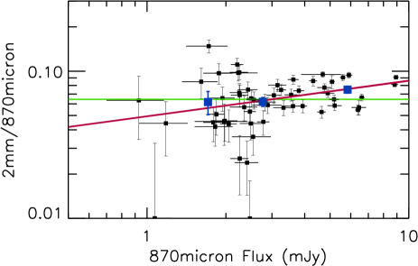
Figure 3: 2 mm to 870 $\mu$m flux density ratio vs. 870 $\mu$m flux density for every source in Table 1 that was observed at 2 mm (black squares). The large blue squares show the means and errors in the means in various flux ranges (see Table 4). The green line shows the median ratio, while the red line shows a power law fit.

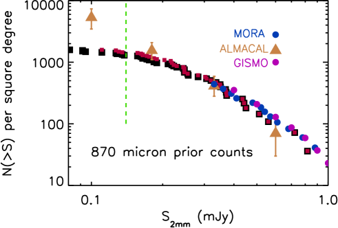
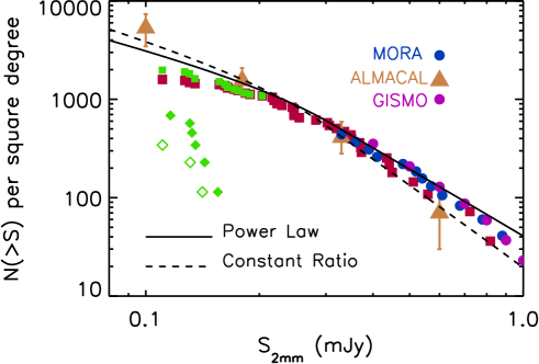
Figure 4: Both panels show our 2 mm cumulative number counts for sources with ALMA 870 $\mu$m priors in the central 100 arcmin² of the GOODS-S. (a) The black squares show the 870 $\mu$m prior-based counts ($>2\sigma$ at 2 mm). These are formally lower limits to the complete counts. The red squares show the $>1.8$ mJy 870 $\mu$m prior-based counts ($>2\sigma$ at 2 mm), corrected for the small fraction of priors without 2 mm observations. The green dashed line shows a flux density of 0.14 mJy above which we expect the 870 $\mu$m prior-based counts to be substantially complete and below which we detect additional sources in the blank field 2 mm images (see text and (b)). (b) The green solid diamonds show the positive blank field-based counts, and the green open diamonds show the negative blank field-based counts. The green solid squares show the combination of the 870 $\mu$m prior-based counts (red squares) and the positive blank field-based counts (using the 50% weighting factor discussed in the text). The black curves show the 850 $\mu$m counts from Hsu et al. (2016) converted to 2 mm using either the median $f_{2\,{\rm mm}}/f_{870\,\mu{\rm m}}$$=0.064$ from Section 3 (dashed) or the power law in Equation 1 (solid). In both panels, we show the IRAM GISMO (Magnelli et al. 2019; purple circles), ALMA MORA (Zavala et al. 2021; blue circles), and ALMACAL (Chen et al. 2023; gold triangles with error bars) blank field-based counts for comparison.

Table 4: Means and Errors

Number	Mean	Mean	Variance	Error in
	$f_{870\,\mu{\rm m}}$	$f_{2\,{\rm mm}}/f_{870\,\mu{\rm m}}$		Mean
	(mJy)
15	5.833	0.075	0.015	0.004
28	2.768	0.062	0.023	0.004
11	1.709	0.062	0.037	0.011

4 Cumulative and Differential Number Counts at 2 mm

In this section, we measure the cumulative and differential number counts at 2 mm. We start with the 2 mm counts corresponding to the 870 $\mu$m sample. Such counts will not be complete, since they are based on only the 870 $\mu$m priors. Moreover, some of these priors do not have 2 mm observations. We will make appropriate corrections below, but here we note that since the 870 $\mu$m sample is highly complete to near 2 mJy, and given the median $f_{2\,{\rm mm}}/f_{870\,\mu{\rm m}}$=0.064 from Section 3, we expect the 2 mm counts will be near-complete to 0.13 mJy.

We take as our 870 $\mu$m priors the 70 sources from Cowie et al. (2018) that lie within the central 100 arcmin² of the field. Fifty-one of these have 2 mm observations. To determine which signal-to-noise threshold to adopt—we already know it can be lower than one would choose for a blank field selection, given our use of priors—we estimate the expected level of spurious 2 mm detections by measuring the flux densities in the 2 mm images at random positions. We find one spurious 2 mm detection if we use a $2\sigma$ threshold, and 0.25 if we use a $2.5\sigma$ threshold. We therefore adopt a $2\sigma$ threshold, which 49 of the 51 sources satisfy.

In Figure 4(a), we show as black squares the cumulative counts for the 49 870 $\mu$m priors detected above a $2\sigma$ threshold at 2 mm. These are formally lower limits to the complete number counts. We form the counts from the number of sources above a given flux density divided by 100 arcmin², the area of our 870 $\mu$m priors.

Next, we correct the counts to allow for the 870 $\mu$m priors that do not have $>2\sigma$ 2 mm flux densities. Of the 50 priors with 870 $\mu$m flux densities above 1.8 mJy in the central 100 arcmin² of the field, 45 have 2 mm observations (see Section 2.1 for why 5 sources were excluded from the 2 mm observations), only one of which is not detected above the $2\sigma$ threshold. We recompute the cumulative number counts for this sample of 50 sources, assigning 2 mm flux densities to the 6 missing sources using their 870 $\mu$m flux densities and the median $f_{2\,{\rm mm}}/f_{870\,\mu{\rm m}}$ $=0.064$. We show these counts as the red squares in Figure 4 (both panels), and we hereafter refer to them as our prior-based 2 mm counts. The correction is small and only appears at the faintest flux densities

In Figure 4 (both panels), we compare our prior-based 2 mm counts with blank field-based 2 mm counts from the literature. The brighter counts come from the IRAM GISMO sample of Magnelli et al. (2019) (purple circles) and the ALMA MORA sample of Zavala et al. (2021) (blue circles). We do not show the GISMO sample of Staguhn et al. (2014), whose counts are high compared with the other literature counts. Note that all of these samples contain a relatively small number of sources ($\lesssim 15$ sources in each). The deeper counts are from the ALMACAL sample of Chen et al. (2023) (gold triangles). Above a 2 mm flux of $0.2$ mJy, our prior-based 2 mm counts agree well with the literature blank field-based 2 mm counts.

In addition to the 2 mm sources found by using our 870 $\mu$m priors, we may look at the blank field images to see if there are any sources not found by using our priors. To do so, we restrict each 2 mm ALMA image to a radius of $28^{\prime\prime}$ for a relatively uniform rms noise of $<0.027$ mJy. Then, after masking the targeted 870 $\mu$m ALMA sources, our 2 mm images provide deep, blank field observations over an area of 32 arcmin². Given the large number of independent beams (just over 50000) in the area, we adopt a fairly high selection threshold of $4.5\sigma$. At this level, we expect about 0.4 false positive sources.

When we search the 32 arcmin² area, we find 6 additional sources with aperture and primary-beam corrected 2 mm flux densities between 0.12 and 0.16 mJy. (Seven of the 870 $\mu$m priors have 2 mm flux densities in this range, six of which have an 870 $\mu$m flux above 1.8 mJy.) We do not attempt to make any corrections for clustering that might bias the sample (e.g., Béthermin et al., 2020). In order to test our false positive estimation, we run the same procedure on the negatives of the images. This yields 3 sources, which suggests that as many as 50% of the additional sources in the images may be spurious. (If we change the selection threshold from $4.5\sigma$ to $5\sigma$, then we have 2 additional sources in the images and none in the negatives of the images.)

We also try to check the reliability of the 6 additional sources in the 2 mm images by looking to see whether any are detected at 1.2 mm or 3 mm. However, only 2 of the 6 are well covered by the 1.2 mm observations. Neither is significantly detected. All 6 are covered by the 3 mm observations, but the 3 mm data are too shallow to provide useful constraints.

In Figure 4(b), we show the cumulative number counts for the additional sources in the images (green solid diamonds) and for those in the negatives of the images (green open diamonds). We use the 50% weighting factor to combine the positive blank field-based counts with the 870 $\mu$m prior-based counts to obtain a final estimate of the counts (green squares).

As discussed in Zavala et al. (2021), cumulative number counts are clearer for these small samples. However, it is easier to show errors when using differential number counts. Thus, in Figure 5, we show the differential counts above 0.14 mJy for our corrected data (black squares). The error bars are 68% confidence Poisson uncertainties on the number of sources in each bin. We compare these with the ALMACAL counts (gold diamonds) (Chen et al., 2023). Above 0.2 mJy, the two samples are consistent within the errors, while below 0.2 mJy, our counts are low compared to ALMACAL. However, their lowest point is based on only 4 sources and hence is quite uncertain.

We also show in Figure 5 the models of Lagos et al. (2020) (blue) and Popping et al. (2020) (green), as taken from Chen et al. (2023). Above 0.2 mJy, these models are broadly consistent with both the ALMACAL and present counts, while below 0.2 mJy, they lie between the two samples.

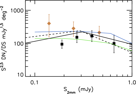
Figure 5: Differential number counts above 0.14 mJy for our corrected data (black squares). The error bars are 68% confidence Poisson uncertainties. The flux density bins are 0.14–0.23, 0.23–0.32, 0.32–0.5, and 0.5–1 mJy, which contain 15, 10, 9, and 4 sources, respectively. The ALMACAL counts (Chen et al., 2023) are shown with gold diamonds. Their faintest bin contains only 4 sources. The black curves show the 850 $\mu$m counts from Hsu et al. (2016) converted to 2 mm using either the median $f_{2\,{\rm mm}}/f_{870\,\mu{\rm m}}$$=0.064$ from Section 3 (dashed) or the power law in Equation 1 (solid). The models of Lagos et al. (2020) and Popping et al. (2020) (taken from Chen et al. 2023) are shown with blue and green curves, respectively.

Ultradeep galaxy number counts, which nearly fully resolve the EBL, have now been obtained at 850 $\mu$m or 870 $\mu$m (e.g., Hsu et al., 2016; Béthermin et al., 2020; Chen et al., 2023) and at 1.1 mm or 1.2 mm (e.g., Fujimoto et al., 2016; Muñoz Arancibia et al., 2018, 2022; González-López et al., 2020). Here we make comparisons with Hsu et al. (2016) by converting their differential number counts, which take the form of a broken power law

$$\frac{dN}{dS}=\left\{\begin{matrix}N_{0}\left(\frac{S}{S_{0}}\right)^{-\alpha}~{}~{}{\rm if}~{}S\leq S_{0}\\ N_{0}\left(\frac{S}{S_{0}}\right)^{-\beta}~{}~{}{\rm if}~{}S>S_{0}\\ \end{matrix}\right.\,,$$ (2)

to 2 mm. For the median $f_{2\,{\rm mm}}/f_{870\,\mu{\rm m}}$=0.064 conversion, $\alpha$ is 2.12, $\beta$ is 3.73, $S_{0}$ is 0.29 mJy, and the normalization, $N_{0}$, is 5340 mJy^-1 deg^-2. For the Equation 1 conversion, $\alpha$ is 1.92, $\beta$ is 3.24, $S_{0}$ is 0.31 mJy, and $N_{0}$ is 4160 mJy^-1 deg^-2. We show these power laws on Figure 5. Above 0.2 mJy, they match well to both the ALMACAL and present counts, while below 0.2 mJy, they lie between the two samples. The power laws are also broadly consistent with the Lagos et al. (2020) and Popping et al. (2020) models.

We then integrate these broken power laws to get the cumulative counts, which we show as black curves in Figure 4(b). These curves provide a good match to all of the 2 mm data.

Above 0.2 mJy, where we expect the sample to be essentially complete based on the 870 $\mu$m selection (see Figure 4), our measured contribution to the 2 mm EBL is $0.63\pm 0.09$ Jy deg^-2. Comparing with the total values of $3.0\pm 5.8$ Jy deg^-2 from Odegard et al. (2019) based on the Planck HFI data and 6 Jy deg^-2 inferred by Chen et al. (2023) by extrapolating the COBE FIRAS data to 2 mm, this corresponds to 10 to 19%. But the uncertainties on the total EBL measurements are substantial.

While recognizing the uncertainties inherent in extrapolating beyond what is measured, we can use the converted Hsu et al. (2016) counts to extrapolate the contribution to the EBL to fainter 2 mm flux densities than measured in order to estimate how faint future 2 mm measurements—such as those that will be made with TolTEC—may need to be to resolve the EBL substantially.

With the median conversion, we would resolve the 2 mm EBL at $\sim 0.004$ mJy, while with the power law conversion, we would need to reach a flux $<0.001$ mJy to resolve substantially the 2 mm EBL. This may be difficult to achieve with TolTEC and may require ALMA observations of lensing clusters, such as those carried out at 1.1 mm or 1.2 mm (e.g., Fujimoto et al., 2016; Muñoz Arancibia et al., 2018; González-López et al., 2020).

We emphasize that these estimates depend on the extrapolation of $f_{2\,{\rm mm}}/f_{870\,\mu{\rm m}}$ well below the values at which they were measured. If there are sources with higher values of this ratio at lower 2 mm flux densities, then the EBL contributions could be higher and the resolution of the 2 mm EBL could occur at higher flux densities.

5 2 mm Based Redshift Estimates

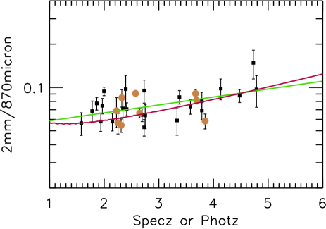
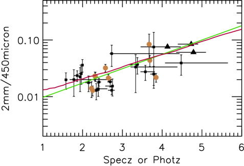
Figure 6: (a) $f_{2\,{\rm mm}}/f_{870\,\mu{\rm m}}$ and (b) $f_{2\,{\rm mm}}/f_{450\,\mu{\rm m}}$ vs. spectroscopic redshift (gold circles) or Straatman et al. (2016) photometric redshift (black symbols; for clarity, we only show the 68% confidence ranges in (b)) for the sources in Table 1 with a corrected aperture flux density above 0.14 mJy. The uncertainties in (a) are dominated by the $f_{2\,{\rm mm}}$ uncertainties, while those in (b) are dominated by the $f_{450\,\mu{\rm m}}$ uncertainties. The upward pointing triangles in (b) show the $1\sigma$ lower limits on the flux ratios for the three sources not detected at 450 $\mu$m. The green curves show power law fits to the data (Equations 3 and 4). The red curves show the flux ratios using Arp 220 as a template for the SED shape (Silva et al., 1998).

As we discussed in the Introduction, one of the primary motivations for pushing to longer wavelengths than 870 $\mu$m is to detect a larger fraction of high-redshift galaxies (see Figure 1(a)). However, this still leaves the problem of determining the redshifts for the detected sources, and, in particular, for the high-redshift galaxies. Many submillimeter or millimeter detected galaxies are too faint for optical/NIR spectroscopic redshifts, or in a small number of cases, even for photometric redshifts. For the 55 sources with measured 2 mm flux densities in Table 1, only 13 have well-determined spectroscopic redshifts. Even including in this count the handful of sources that were not observed at 2 mm because they had existing spectroscopic redshifts, less than a third of all the observed sources have spectroscopic redshifts. No source in Table 1 has a spectroscopic redshift greater than 4.

Ideally, one can measure redshifts using spectral observations in the millimeter, as we have done for some of the brighter 2 mm sources in our sample (F. Bauer et al. 2023, in preparation), and as ASPECS has done for several of the slightly fainter sources (González-López et al., 2019). Alternatively, one can estimate redshifts by fitting to the entire FIR SED (e.g., Battisti et al., 2019; Dudzevičiūtė et al., 2020). This was done for the present sample in Cowie et al. (2018), though this type of analysis does have uncertainties due to redshift degeneracies with the temperatures of the dust SEDs (e.g., Casey et al., 2019; Jin et al., 2019; Cortzen et al., 2020).

Redshifts can also be roughly estimated using submillimeter or millimeter flux ratios, which allow one to work with much more limited data. Here we focus on the purely empirical relation between measured flux ratio (from the present 450 $\mu$m, 850 $\mu$m, and 2 mm data) and spectroscopic or photometric redshift (estimated from optical/NIR data). The 2 mm data improve these estimates by providing a wider wavelength separation.

In Figure 6, we plot for the sources with a 2 mm flux density above 0.14 mJy (all of these are detected above $3\sigma$) (a) $f_{2\,{\rm mm}}/f_{870\,\mu{\rm m}}$ and (b) $f_{2\,{\rm mm}}/f_{450\,\mu{\rm m}}$ versus available spectroscopic (gold circles) or photometric (black) redshift. Fitting the ratios versus redshift with error-weighted power law fits (green curves) gives, respectively,

$$\log(f_{2\,{\rm mm}}/f_{870\,\mu{\rm m}})=0.067z-1.400$$ (3)

and

$$\log(f_{2\,{\rm mm}}/f_{450\,\mu{\rm m}})=0.268z-2.319\,.$$ (4)

Bisector fits give almost identical results, with the right-hand side of Equation 3 becoming $0.065z-1.329$, and the right-hand side of Equation 4 becoming $0.278z-2.361$.

For $f_{870~{}\mu{\rm m}}/f_{450~{}\mu{\rm m}}$, the power law fit is almost identical to that given in Barger et al. (2022), namely,

$$\log(f_{870\,\mu{\rm m}}/f_{450\,\mu{\rm m}})=0.16z-0.96\,,$$ (5)

which was based on both this field (though the 450 $\mu$m data were not as deep) and the GOODS-N.

Unfortunately, the dependence of $f_{2\,{\rm mm}}/f_{870\,\mu{\rm m}}$ on redshift is too shallow, especially given the dispersion, for it to be useful in estimating redshifts. However, $f_{2\,{\rm mm}}/f_{450\,\mu{\rm m}}$ has a steeper dependence on redshift and hence can provide better redshift estimates than $f_{870~{}\mu{\rm m}}/f_{450~{}\mu{\rm m}}$. Both of these estimates depend on the passage of the 450 $\mu$m band through the rest-frame peak 100 $\mu$m region; thus, they are critically dependent on the short-wavelength data.

As we illustrate in Figure 7, the $f_{2\,{\rm mm}}/f_{450\,\mu{\rm m}}$ color-predicted redshift for the sources with a 2 mm flux density above 0.14 mJy is correlated with the spectroscopic and photometric redshift samples, with a similar spread for both. We show uncertainties on the color-predicted redshifts that correspond to the 68% range in the flux density ratio. Within these uncertainties, only five of the sources (7, 26, 41, 52, and 58 in Table 1) could lie at $z>5$. However, source 7, which has a color-predicted redshift range from 3.98 to 5.80, has a CO redshift of 3.672 (Table 2).

This leaves only four sources that could lie at $z>5$ based on the color-predicted redshifts. The photometric redshifts for these four sources are between 3.8 and 4.8. Since the photometric redshift for source 26 is robust ($Q<3$), we do not consider it further as a $z>5$ candidate. However, the photometric redshifts for the remaining sources are considered to be of poorer quality ($Q>3$), leaving us with a total of three $z>5$ candidates.

Note that only one source has a $z_{\rm phot}>5$ (source 45): Straatman et al. (2016) give $z_{\rm phot}=7.62$ ($Q>3$), while Santini et al. (2015) give $z_{\rm phot}=6.62$. However, this is a poorly determined photometric redshift, and the color-predicted redshift is more consistent with a $z<3.5$ solution (see Figure 7).

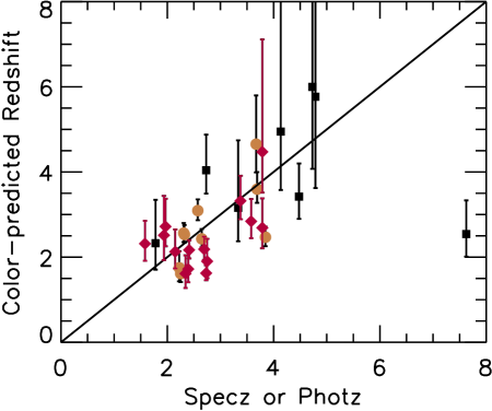
Figure 7: Color-predicted redshift based on $f_{2\,{\rm mm}}/f_{450\,\mu{\rm m}}$ vs. spectroscopic redshift (gold circles) or Straatman et al. (2016) photometric redshift (red diamonds for robust $Q<3$, and black squares for poorer quality $Q>3$) for the sources in Table 1 with $f_{2\,{\rm mm}}$ $>0.14$ mJy. All errors are 68% confidence.

As we illustrate in Figure 8, there is no strong dependence of redshift on $f_{2\,{\rm mm}}$. A bisector fit gives a weak gradient of $z=3.38+0.64\log$ $f_{2\,{\rm mm}}$, with the brighter sources being at a slightly higher redshift. However, a Mann-Whitney test comparing the $f_{2\,{\rm mm}}$ $>0.33$ mJy sample with the $f_{2\,{\rm mm}}$ $=$ 0.14–0.33 mJy sample gives a $p$ value of 0.74, so the two distributions are not significantly different at the 0.05 level. The bisector fit is shallower than the model in Figure 3 of Béthermin et al. (2015), but given the small range in flux density, and the uncertainties in the slope, it could be broadly consistent.

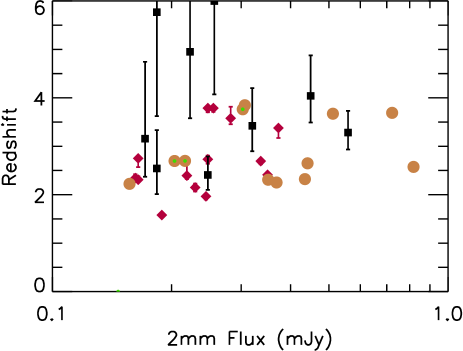
Figure 8: Redshift vs. $f_{2\,{\rm mm}}$ for the sources in Table 1 with $f_{2\,{\rm mm}}$  $>0.14$ mJy. Black squares show color-predicted redshifts based on $f_{2\,{\rm mm}}/f_{450\,\mu{\rm m}}$, while gold circles show sources with spectroscopic redshifts and red diamonds show sources with Straatman et al. (2016) photometric redshifts (robust $Q<3$ only). All errors are 68% confidence. We have included three sources using $0.064\times$$f_{870\,\mu{\rm m}}$ where $f_{2\,{\rm mm}}$ was not measured (central green circles)

In Cowie et al. (2018), we determined star formation rates (SFRs) for the ALMA 870 $\mu$m sample using MAGPHYS (da Cunha et al., 2015). In MAGPHYS, SFRs are computed for a Chabrier (2003) initial mass function (IMF). However, since there is a near-constant dependence of SFR on 2 mm flux (see Figure 1(a)), we can also simply estimate the SFR from the 2 mm flux. Doing a linear fit to the MAGPHYS SFRs versus the 2 mm flux gives SFR $=1750\times$($f_{2\,{\rm mm}}$ in mJy) M_⊙ yr^-1, which we adopt here.

We can compare this with estimates in the literature of the relation between SFR and 850 $\mu$m flux (converted to a Chabrier IMF) using $f_{2\,{\rm mm}}/f_{870\,\mu{\rm m}}$ = 0.064. These give SFR $=1970\times$($f_{2\,{\rm mm}}$ in mJy) M_⊙ yr^-1 (Barger et al., 2014) and SFR $=2100\times$($f_{2\,{\rm mm}}$ in mJy) M_⊙ yr^-1 (Cowie et al., 2017), which are reasonably consistent with the relation in the previous paragraph, given the uncertainties.

Numerous estimates of the dusty star formation history have been made from submillimeter observations (e.g., Barger et al., 2000, 2014; Chapman et al., 2005; Wardlow et al., 2011; Casey et al., 2013; Swinbank et al., 2014; Cowie et al., 2017). However, determining the contributions of dusty galaxies at very high redshifts has been challenging. Here we focus on whether the 2 mm data find significant star formation at high redshifts (here $z>5$), and we make comparisons with the 2 mm results of Zavala et al. (2021) and Cooper et al. (2022).

Using the SFR estimated from the 2 mm flux and the spectroscopic, photometric $(Q<3)$, or else $f_{2\,{\rm mm}}/f_{450\,\mu{\rm m}}$ color-predicted redshift (see Figure 8), we can estimate the star formation history. The 2 mm flux limit of 0.14 mJy corresponds to a SFR of 250 M_⊙ yr^-1. Above this limit, we find the SFR densities given in Table 5. These values are considerably higher than those given in Cooper et al. (2022) due to the depth of our observations. We find a peak in the $z=2$–3 range and a rapid drop-off to the highest redshifts.

Even if we place all three $z>5$ candidates at these redshifts, they only contain about 6% of the star formation of all the DSFGs observed in the area (1200 M_⊙ yr^-1 versus 19000 M_⊙ yr^-1). This is a smaller contribution than claimed by Zavala et al. (2021) at such high redshifts ($\sim 35$% at $z=5$ and 20–25% in the redshift range $z=$ 6–7). We conclude that only a very small fraction of DSFG formation occurs at high redshift.

Table 5: SFR Densities

Redshift	SFR Density	68% Confidence
	(M⊙ yr-1 Mpc-3)
1.2–2	0.003	0.001–0.007
2–3	0.028	0.022–0.036
3–4	0.023	0.016–0.032
4–5	0.004	0.001–0.010
5–6	0.003	0.001–0.007

6 Summary

Starting from an ALMA 870 $\mu$m sample in the GOODS-S obtained from targeted observations of SCUBA-2 850 $\mu$m sources, we made ALMA spectral line scans that provide 2 mm continuum observations down to below a 2 mm flux density of 0.1 mJy. We also deepened our SCUBA-2 450 $\mu$m observations of the field. Our primary results are as follows.

(1) Using every source that we observed at 2 mm, we found a median $f_{2\,{\rm mm}}/f_{870\,\mu{\rm m}}$ of 0.064 (the mean ratio is 0.066 with an error of 0.003 and determined a bisector power law fit to $\log$($f_{2\,{\rm mm}}/f_{870\,\mu{\rm m}}$) versus $\log$($f_{870\,\mu{\rm m}}$). We used these to convert 870 $\mu$m flux densities to 2 mm.

(2) We measured the cumulative and differential number counts at 2 mm using the 870 $\mu$m sources as priors. We corrected the counts for the small number of sources without $>2\sigma$ 2 mm flux densities. We also searched for additional 2 mm sources not found by our priors. After estimating the number of false positives by searching for sources in the negatives of the images, we corrected the counts. We determined that our cumulative and differential 2 mm number counts are in reasonable agreement with the literature above 0.2 mJy.

(3) Above 0.2 mJy, we measured a contribution to the 2 mm EBL of $0.63\pm 0.09$ Jy deg^-2, which corresponds to 10 to 19% of the total EBL given by Odegard et al. (2019) and Chen et al. (2023), respectively, but the uncertainties on these values are substantial. While recognizing the uncertainties inherent in extrapolating beyond what is measured, we estimated that in order to resolve the 2 mm EBL substantially, 2 mm flux density measurements below 0.004 mJy—and possibly as faint as 0.001 mJy—will need to be reached.

(4) We determined that the 2 mm to 450 $\mu$m flux density ratio provides an estimate of the spectroscopic and photometric redshifts of the sources. We found no significant dependence of the redshifts on the 2 mm flux density for sources with 2 mm flux densities between 0.14 and 1 mJy.

(5) We only identified three galaxies that may lie at $z>5$. Our observations measure galaxies with SFRs in excess of 250 M_⊙ yr^-1. For these galaxies, the SFR densities fall by a factor of $\sim 9$ from $z=2$–3 to $z=5$–6.

References

- Adam et al. (2018) Adam, R., Adane, A., Ade, P. A. R., et al. 2018, A&A, 609, A115
- Aravena et al. (2020) Aravena, M., Boogaard, L., Gónzalez-López, J., et al. 2020, ApJ, 901, 79
- Barger et al. (2022) Barger, A. J., Cowie, L. L., Blair, A. H., & Jones, L. H. 2022, ApJ, 934, 56
- Barger et al. (2000) Barger, A. J., Cowie, L. L., & Richards, E. A. 2000, AJ, 119, 2092
- Barger et al. (2012) Barger, A. J., Wang, W. H., Cowie, L. L., et al. 2012, ApJ, 761, 89
- Barger et al. (2014) Barger, A. J., Cowie, L. L., Chen, C. C., et al. 2014, ApJ, 784, 9
- Battisti et al. (2019) Battisti, A. J., da Cunha, E., Grasha, K., et al. 2019, ApJ, 882, 61
- Béthermin et al. (2015) Béthermin, M., De Breuck, C., Sargent, M., & Daddi, E. 2015, A&A, 576, L9
- Béthermin et al. (2010) Béthermin, M., Dole, H., Cousin, M., & Bavouzet, N. 2010, A&A, 516, A43
- Béthermin et al. (2020) Béthermin, M., Fudamoto, Y., Ginolfi, M., et al. 2020, A&A, 643, A2
- Brammer et al. (2008) Brammer, G. B., van Dokkum, P. G., & Coppi, P. 2008, ApJ, 686, 1503
- Casey et al. (2011) Casey, C. M., Chapman, S. C., Smail, I., et al. 2011, MNRAS, 411, 2739
- Casey et al. (2013) Casey, C. M., Chen, C.-C., Cowie, L. L., et al. 2013, MNRAS, 436, 1919
- Casey et al. (2019) Casey, C. M., Zavala, J. A., Aravena, M., et al. 2019, ApJ, 887, 55
- Casey et al. (2021) Casey, C. M., Zavala, J. A., Manning, S. M., et al. 2021, ApJ, 923, 215
- Chabrier (2003) Chabrier, G. 2003, PASP, 115, 763
- Chapman et al. (2005) Chapman, S. C., Blain, A. W., Smail, I., & Ivison, R. J. 2005, ApJ, 622, 772
- Chen et al. (2013) Chen, C.-C., Cowie, L. L., Barger, A. J., et al. 2013, ApJ, 776, 131
- Chen et al. (2023) Chen, J., Ivison, R. J., Zwaan, M. A., et al. 2023, MNRAS, 518, 1378
- Cooper et al. (2022) Cooper, O. R., Casey, C. M., Zavala, J. A., et al. 2022, ApJ, 930, 32
- Cortzen et al. (2020) Cortzen, I., Magdis, G. E., Valentino, F., et al. 2020, A&A, 634, L14
- Cowie et al. (2022) Cowie, L. L., Barger, A. J., Bauer, F. E., et al. 2022, ApJ, 939, 5
- Cowie et al. (2017) Cowie, L. L., Barger, A. J., Hsu, L. Y., et al. 2017, ApJ, 837, 139
- Cowie et al. (2009) Cowie, L. L., Barger, A. J., Wang, W. H., & Williams, J. P. 2009, ApJ, 697, L122
- Cowie et al. (2018) Cowie, L. L., González-López, J., Barger, A. J., et al. 2018, ApJ, 865, 106
- da Cunha et al. (2015) da Cunha, E., Walter, F., Smail, I. R., et al. 2015, ApJ, 806, 110
- Davé et al. (2019) Davé, R., Anglés-Alcázar, D., Narayanan, D., et al. 2019, MNRAS, 486, 2827
- Dudzevičiūtė et al. (2020) Dudzevičiūtė, U., Smail, I., Swinbank, A. M., et al. 2020, MNRAS, 494, 3828
- Dunlop et al. (2017) Dunlop, J. S., McLure, R. J., Biggs, A. D., et al. 2017, MNRAS, 466, 861
- Fixsen et al. (1998) Fixsen, D. J., Dwek, E., Mather, J. C., Bennett, C. L., & Shafer, R. A. 1998, ApJ, 508, 123
- Franco et al. (2018) Franco, M., Elbaz, D., Béthermin, M., et al. 2018, A&A, 620, A152
- Fujimoto et al. (2016) Fujimoto, S., Ouchi, M., Ono, Y., et al. 2016, ApJS, 222, 1
- Gómez-Guijarro et al. (2022) Gómez-Guijarro, C., Elbaz, D., Xiao, M., et al. 2022, A&A, 658, A43
- González-López et al. (2017) González-López, J., Bauer, F. E., Romero-Cañizales, C., et al. 2017, A&A, 597, A41
- González-López et al. (2019) González-López, J., Decarli, R., Pavesi, R., et al. 2019, ApJ, 882, 139
- González-López et al. (2020) González-López, J., Novak, M., Decarli, R., et al. 2020, ApJ, 897, 91
- Hatsukade et al. (2018) Hatsukade, B., Kohno, K., Yamaguchi, Y., et al. 2018, PASJ, 70, 105
- Hodge et al. (2013) Hodge, J. A., Karim, A., Smail, I., et al. 2013, ApJ, 768, 91
- Holland et al. (2013) Holland, W. S., Bintley, D., Chapin, E. L., et al. 2013, MNRAS, 430, 2513
- Hsu et al. (2016) Hsu, L.-Y., Cowie, L. L., Chen, C.-C., Barger, A. J., & Wang, W.-H. 2016, ApJ, 829, 25
- Hurley et al. (2017) Hurley, P. D., Oliver, S., Betancourt, M., et al. 2017, MNRAS, 464, 885
- Inami et al. (2017) Inami, H., Bacon, R., Brinchmann, J., et al. 2017, A&A, 608, A2
- Jin et al. (2019) Jin, S., Daddi, E., Magdis, G. E., et al. 2019, ApJ, 887, 144
- Kriek et al. (2015) Kriek, M., Shapley, A. E., Reddy, N. A., et al. 2015, ApJS, 218, 15
- Kurk et al. (2013) Kurk, J., Cimatti, A., Daddi, E., et al. 2013, A&A, 549, A63
- Lagos et al. (2020) Lagos, C. d. P., da Cunha, E., Robotham, A. S. G., et al. 2020, MNRAS, 499, 1948
- Magnelli et al. (2019) Magnelli, B., Karim, A., Staguhn, J., et al. 2019, ApJ, 877, 45
- McMullin et al. (2007) McMullin, J. P., Waters, B., Schiebel, D., Young, W., & Golap, K. 2007, in Astronomical Society of the Pacific Conference Series, Vol. 376, Astronomical Data Analysis Software and Systems XVI, ed. R. A. Shaw, F. Hill, & D. J. Bell, 127
- Mignoli et al. (2005) Mignoli, M., Cimatti, A., Zamorani, G., et al. 2005, A&A, 437, 883
- Muñoz Arancibia et al. (2018) Muñoz Arancibia, A. M., González-López, J., Ibar, E., et al. 2018, A&A, 620, A125
- Muñoz Arancibia et al. (2022) —. 2022, arXiv e-prints, arXiv:2203.06195
- Odegard et al. (2019) Odegard, N., Weiland, J. L., Fixsen, D. J., et al. 2019, ApJ, 877, 40
- Oesch et al. (2023) Oesch, P. A., Brammer, G., Naidu, R. P., et al. 2023, arXiv e-prints, arXiv:2304.02026
- Popping et al. (2020) Popping, G., Walter, F., Behroozi, P., et al. 2020, ApJ, 891, 135
- Puget et al. (1996) Puget, J. L., Abergel, A., Bernard, J. P., et al. 1996, A&A, 308, L5
- Santini et al. (2015) Santini, P., Ferguson, H. C., Fontana, A., et al. 2015, ApJ, 801, 97
- Schaye et al. (2015) Schaye, J., Crain, R. A., Bower, R. G., et al. 2015, MNRAS, 446, 521
- Serjeant et al. (2003) Serjeant, S., Dunlop, J. S., Mann, R. G., et al. 2003, MNRAS, 344, 887
- Shimizu et al. (2012) Shimizu, I., Yoshida, N., & Okamoto, T. 2012, MNRAS, 427, 2866
- Silva et al. (1998) Silva, L., Granato, G. L., Bressan, A., & Danese, L. 1998, ApJ, 509, 103
- Smail et al. (2021) Smail, I., Dudzevičiūtė, U., Stach, S. M., et al. 2021, MNRAS, 502, 3426
- Stach et al. (2019) Stach, S. M., Dudzevičiūtė, U., Smail, I., et al. 2019, MNRAS, 487, 4648
- Staguhn et al. (2014) Staguhn, J. G., Kovács, A., Arendt, R. G., et al. 2014, ApJ, 790, 77
- Straatman et al. (2016) Straatman, C. M. S., Spitler, L. R., Quadri, R. F., et al. 2016, ApJ, 830, 51
- Swinbank et al. (2014) Swinbank, A. M., Simpson, J. M., Smail, I., et al. 2014, MNRAS, 438, 1267
- Szokoly et al. (2004) Szokoly, G. P., Bergeron, J., Hasinger, G., et al. 2004, ApJS, 155, 271
- Wang et al. (2009) Wang, W.-H., Barger, A. J., & Cowie, L. L. 2009, ApJ, 690, 319
- Wang et al. (2006) Wang, W. H., Cowie, L. L., & Barger, A. J. 2006, ApJ, 647, 74
- Wang et al. (2017) Wang, W.-H., Lin, W.-C., Lim, C.-F., et al. 2017, ApJ, 850, 37
- Wardlow et al. (2011) Wardlow, J. L., Smail, I., Coppin, K. E. K., et al. 2011, MNRAS, 415, 1479
- Wilson et al. (2020) Wilson, G. W., Abi-Saad, S., Ade, P., et al. 2020, in Society of Photo-Optical Instrumentation Engineers (SPIE) Conference Series, Vol. 11453, Society of Photo-Optical Instrumentation Engineers (SPIE) Conference Series, 1145302
- Zavala et al. (2017) Zavala, J. A., Aretxaga, I., Geach, J. E., et al. 2017, MNRAS, 464, 3369
- Zavala et al. (2021) Zavala, J. A., Casey, C. M., Manning, S. M., et al. 2021, ApJ, 909, 165