Stability of implicit neural networks for long-term forecasting in dynamical systems

Abstract

Forecasting physical signals in long time range is among the most challenging tasks in Partial Differential Equations (PDEs) research. To circumvent limitations of traditional solvers, many different Deep Learning methods have been proposed. They are all based on auto-regressive methods and exhibit stability issues. Drawing inspiration from the stability property of implicit numerical schemes, we introduce a stable auto-regressive implicit neural network. We develop a theory based on the stability definition of schemes to ensure the stability in forecasting of this network. It leads us to introduce hard constraints on its weights and propagate the dynamics in the latent space. Our experimental results validate our stability property, and show improved results at long-term forecasting for two transports PDEs.

1 Introduction and motivation

Numerical simulations are one of the main tools to study systems described by PDEs, which are essential for many applications including, e.g., fluid dynamics and climate science. However, solving these systems and even more using them to predict long term phenomenon remains a complex challenge, mainly due to the accumulation of errors over time. To overcome the limitations of traditional solvers and to exploit the available data, many different deep learning methods have been proposed.

For the task of forecasting spatio-temporal dynamics, Ayed et al. (2019) used a standard residual network with convolutions and Sorteberg et al. (2019); Lino et al. (2020); Fotiadis et al. (2020) used Long short-term memory (LSTM) and Convolutional neural network (CNN) for the wave equation. In Wiewel et al. (2019); Kim et al. (2019), a good performances is obtained by predicting within the latent spaces of neural networks. More recently, Brandstetter et al. (2022) used graph neural networks with several tricks and showed great results for forecasting PDEs solutions behavior. Importantly, these methods all solve the PDE iteratively, meaning that they are auto-regressive, the output of the model is used as the input for the next time step. Another line of recent methods that have greatly improved the learning of PDE dynamics are Neural Operators (Li et al., 2020b). These methods can be used as operators or as auto-regressive methods to forecast. However, when used as operators, they do not generalize well beyond the times seen during training. Crucially, these auto-regressive methods tend to accumulate errors over time with no possible control, and respond quite poorly in case of change in the distribution of the data. This leads to stability problems, especially over long periods of time beyond the training horizon.

In the numerical analysis community, the stability issue has been well studied and is usually dealt with implicit schemes. By definition, they imply to solve an equation to go from a time step to the next one but they are generally more stable than explicit schemes. This can be seen on the test equation $\frac{\mathrm{d}y}{\mathrm{d}t}=\lambda y$, where Euler implicit schemes are always stable while Euler explicit schemes are not. Interpreting residual neural networks as numerical schemes, one can apply such schemes and gain theoretical insights on the properties of neural networks. This has already been done in various forms in Haber and Ruthotto (2017); Chen et al. (2018), but not applied to forecasting. Moreover, these works use either the stability of the underlying continuous equation or the stability of the numerical scheme on the test equation and its derivatives, which is not the stability of the numerical scheme on the studied equation. Since a network is discrete, the latter is the most relevant.

We therefore use the stability in norm of schemes, as defined in 2.1. In deep learning (DL), this definition has only been applied to image classification problems (Zhang and Schaeffer, 2020). To the best of our knowledge, this work is the first attempt to forecast PDEs with neural networks using stability as studied in the numerical analysis community.

Using implicit schemes in DL has already been done in different contexts. The earliest line of works tackles image problems, with Haber et al. (2019) designing semi-implicit ResNets and Li et al. (2020a); Shen et al. (2020); Reshniak and Webster (2021) designing different implicit ResNets. The second line of works focuses on dynamical problems. In this way, Nonnenmacher and Greenberg (2021) designed linear implicit layers, which learn and solve linear systems, and Horie and Mitsume (2022) used an implicit scheme as part of an improvement of graph neural network solvers to improve forecasting generalization with different boundary condition shapes. Tackling different types of problems, none of these methods guarantees the forecast stability. For our analysis, we restrict ourselves to ResNet-type networks, i.e., networks with residual connections. We introduce hard constraints on the weights of the network and predict within the latent space of our network. Hence, by modifying the classic implicit ResNet architecture, our method can forecast dynamical system at long range without diverging. We apply these theoretical constraints in our architecture to two 1D transport problems: the Advection equation and Burgers’ equation.

To better investigate networks stability, we perform our experiments under the following challenging setting: for training, we only give to the networks the data from $t=0$ to a small time $t=\Delta t$, and consider the results in forecasting in the long time range at $t=N\cdot\Delta t$, with $N\gg 1$. Note that our setting is harder that the conventional setting presented for e.g. in Brandstetter et al. (2022). Indeed, we only use changes between a single time step for training.

2 Method

To guarantee structural forecasting stability, we take inspiration from implicit schemes. We focus our study on an implicit ResNet with a ReLU activation function. In our approach, an equation is solved at each layer, namely $x_{n+1}:=x_{n}+R_{n}(x_{n+1})$ with $x$ in $\mathbb{R}^{M}$ and $n$ in $\mathbb{N}$ and $R_{n}(x)=\text{ReLU}(W_{n}x+b_{n})$ where $W_{n}$ is upper triangular. The latter constraint is motivated below.

2.1 Implicit ResNet stability analysis

To ensure that our proposed architecture is well-defined, we need to solve $x=x_{n}+R_{n}(x)$. This equation has a solution, as proven in El Ghaoui et al. (2019) and detailed in Appendix 5.1. We can then study its stability. The recursion defining $(x_{n})_{n\in\mathbb{N}}$ reads as an implicit Euler scheme with a step size of 1. As described in the introduction, an implicit scheme is usually more stable than an explicit one. We first recall the definition of stability for schemes. This property ensures that our architecture has an auto-regressive stability.

Definition 2.1 (Stability in norm).

A scheme $(x_{n})_{n\in\mathbb{N}}$ of dimension $M$ is stable in norm $L^{p}$ if there exists $C(T)$ independent of the time discretization step $\Delta t$ such that:

$$\forall~{}x_{0}\in\mathbb{R}^{M},~{}n\geq 0;~{}n\Delta t\leq T,\text{ }\lVert x_{n}\rVert_{p}\leq C(T)\lVert x_{0}\rVert_{p}\text{ .}$$

This general definition of stability in norm ensures that a scheme does not amplify errors. This definition is equivalent to several others in the numerical analysis community.
Suppose that the spectrum of $W_{n}$ is contained in $[-1,0[$ for every integer $n$, we can assert that $(x_{n})_{n\in\mathbb{N}}$ is well-defined, using theorem 5.2. The proof of the stability of our Implicit ResNet network is then by induction on the dimension and is given in appendix 5.4:

Theorem 2.1 (Stability theorem).

If the elements of the diagonal of $W_{n}$ are in $[-1,0)$ for every integer $n$, then $(x_{n})_{n\in\mathbb{N}}$ is stable in norm $L^{p}$.

This theorem leads to hard constraints on the weights of the network.

2.2 Implementation

To validate practically our theoretical results, we choose a setting that highlights stability issues. We then test our implementation of an implicit ResNet. In order to respect the assumptions of theorem 2.1, we forecast the dynamics in the latent space, as detailed below.

Setting

We first learn the trajectory at a given small time step $\Delta t$. We only give data $t=0$ to $t=\Delta t$ for the training. We then forecast in long-term, at $N\cdot\Delta t$ with $N\gg 1$. This very restricted setting allows us to see how the network will react in forecasting with changes in the distribution and error accumulation. Usually neural network forecasting methods use data from $t=0$ to $T=L\cdot\Delta t$ for the training which allows to use different tricks to stabilize the network, such as predicting multiple time steps at the same time. However, in this work, we want to analyze how the network behaves without any trick that can slow down divergence. Indeed, the tricks used in the other settings do not actually guarantee stability of the network. The training is performed with a mean-squared error (MSE) loss.

Implicit neural network architecture

To implement a neural network from Theorem 2.1, we use the following architecture; $z_{\Delta t}=f_{dec}\circ f_{res}^{K}\circ...\circ f_{res}^{1}\circ f_{enc}(z_{0})$, with $f_{res}^{k}(x)=x+\text{ReLU}(W_{k-1}\cdot f_{res}^{k}(x)+b_{k-1})$. The encoder and decoder are linear, and the encoder projects the data to a smaller dimension $M$. The full architecture is illustrated in Figure 2. The specificity of our architecture is that the residual blocks are connected with an implicit Euler scheme iteration. To do so, we use a differentiable root-finding algorithm (Kasim and Vinko, 2020). More precisely, we use the first Broyden method van de Rotten and Lunel (2005) to solve the root-finding problem. It is a quasi-Newton method. This helped getting better results compared to other algorithms.

Latent space forecasting

As in Wiewel et al. (2019); Kim et al. (2019), the forecast can be done within the latent space of the network; $z_{N\cdot\Delta t}=f_{dec}\circ f_{block}\circ...\circ f_{block}\circ f_{enc}(z_{0})$, with $f_{block}=f_{res}^{K}\circ...\circ f_{res}^{1}$. To predict at time $N\cdot\Delta t$ from time $t=0$, we apply $N$ times the residual blocks. It is illustrated in Figure 4. This propagation allows our network to respect the assumptions of theorem 2.1 and thus be stable.

3 Experiments

We evaluate the performance of our method on the Advection equation and Burgers’ equation.

Datasets

Advection equation. We construct our first dataset with the following 1-D linear PDE, $\frac{\partial\psi}{\partial t}=-\frac{1}{4}\frac{\partial\psi}{\partial z},z\in(0,2\pi),\,t\in\mathbb{R}^{+}$ and $\psi(z,0)=f_{0}(z),z\in(0,2\pi)$.

Burgers’ equation. In the second dataset, we consider the following 1-D non-linear PDE,
$\frac{\partial\psi}{\partial t}=-\frac{1}{2}\frac{\partial\psi^{2}}{\partial z}+\frac{\partial^{2}\psi^{2}}{\partial z},z\in(0,2\pi),\,t\in(0,1]$ and $\psi(z,0)=f_{0}(z),z\in(0,2\pi)$.
Both equations have periodic boundary conditions. We approximate the mapping from the initial condition $f_{0}$ to the solution at a given discretization time $\Delta t$, i.e. $u_{0}\mapsto u(\cdot,\Delta t)$. We then forecast to longer time ranges. $\Delta t$ is set to 1 for the Advection equation with a grid of 100 points and 0.0005 for Burgers’ equation with a grid of 128 points.

Baseline methods

We compare our Implicit ResNet with respect to an Explicit ResNet with ReLU activation function and a Fourier Neural Operator (FNO) (Li et al., 2020b). We have also implemented two Explicit ResNet, with a tanh activation function and with batch normalization. We design the Explicit ResNet in the same way as our implicit version, with $K$ layers of residual blocks that are linked by $x_{n+1}=x_{n}+R_{n}(x_{n})$. Traditional methods forecast by using the output of the network at time $t$ to predict the dynamics at time $t+\Delta t$. So to predict at time $N\cdot\Delta t$ from time $t=0$, the baseline networks are iteratively applied $N$ times, as illustrated in Figure 3.

Results

Prediction errors are reported in Table 3 for the Advection equation and Burgers’ equation. We also show the error according to the forecast time in Figure 1.

We found that traditional deep learning methods diverge with the forecast time. They reach a MSE of more than $10^{8}$ for the Advection equation and go to infinity for Burgers’ equation, respectively at time $400$ and $0.15$. Moreover, we see in Figure 1 that their curve in time is convex, so the increase in error is accelerating over time. We also found that our proposed Implicit ResNet presents better results by several orders of magnitude for both datasets. Moreover, we can see in Figure 1 that its curve in time is reaching a stable plateau, as expected from our theorem 2.1.

As for the training, traditional deep learning methods manage to learn very well the dynamics at $t=\Delta t$, with two orders of magnitude better than our Implicit ResNet. However, the latter still manages to learn well the dynamics with a MSE of $10^{-2}$ for the Advection equation and $10^{-3}$ for Burgers’ equation. This difference in training can mainly be explained by the longer training time of the Implicit ResNet, which made us take a smaller number of epochs for this network (1250 against 2500).

Table 1: Results of our approach compared to baselines on the Advection equation and Burgers’ equation. We calculate the means and standard deviations of MSE for each model based on 5 runs with different seeds. The mid-range time is 40 for the Advection equation and 0.075 for Burgers’ and the long range time is respectively 400 and 0.15. Recall that $\Delta t_{adv}=1$ and $\Delta t_{bur}=0.0005$.

		Model	Train Error ($\times 10^{-4}$)	Test Error ($\times 10^{-4}$)	Forecast error at mid-range $T_{adv}=40\cdot\Delta t_{adv}$ $T_{bur}=150\cdot\Delta t_{bur}$	Forecast error at long-range $T_{adv}=400\cdot\Delta t_{adv}$ $T_{bur}=300\cdot\Delta t_{bur}$
Advection		Explicit Res Net	0.03 ± 0.01	0.09 ± 0.07	0.25 ± 0.33	$4.7\cdot 10^{31}$ ± $1.0\cdot 10^{32}$
		FNO	0.04 ± 0.01	0.1 ± 0.08	0.03 ± 0.04	$4.7\cdot 10^{8}$ ± $1.0\cdot 10^{9}$
		Implicit ResNet (Ours)	14.0 ± 9.0	25.0 ± 27.0	27.4 ± 24.0	27.5 ± 24.2
Burgers’		Explicit Res Net	0.17 ± 0.03	0.90 ± 0.38	$2.77\cdot 10^{19}$ ± $6.2\cdot 10^{19}$	$+\infty$
		FNO	0.02 ± 0.002	0.03 ± 0.006	$5.31\cdot 10^{10}$ ± $11.2\cdot 10^{10}$	$+\infty$
		Implicit ResNet (Ours)	4.90 ± 0.64	7.91 ± 0.30	0.67 ± 0.43	0.66 ± 0.44

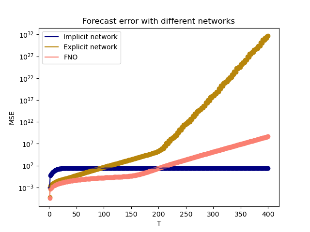
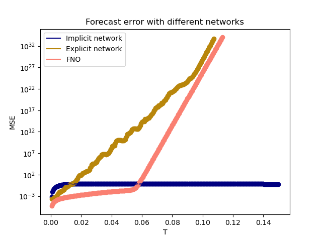
Figure 1: Forecast error for different neural network architectures for the Advection equation (left) and Burger’s equation (right).

Discussion

Figure 1 demonstrates the main benefits of our constrained implicit neural network. Our network is stable whereas the other methods diverge in time. However, although being stable and far better than the baselines, it does not manage to forecast accurately the long-term dynamics. This is further confirmed by Table 7.4, which shows high relative errors. Said otherwise, when stability is guaranteed, convergence is not. We can also note that constraining the weights makes our network harder to train, but guarantees structural forecasting stability.

4 Conclusion

In this work, we studied the challenging task of long-term forecasting in dynamical systems. To do so, we developed a theoretical framework to analyze the stability of deep learning methods for forecasting dynamical systems. We then designed a constrained implicit neural network out of this framework. To the best of our knowledge, this is the first work that proposes to study deep learning architectures for forecasting dynamical systems from a numerical schema standpoint. We showed improved results with respect to deep learning baselines for two transport PDEs.

This work opens new perspectives to study neural networks forecasting stability from a numerical schema standpoint, thus offering more robust architectures. However, this analysis still needs improvements. Even though it ensures forecasting stability of our proposed network, it does not guarantee good convergence properties. We believe that developing this line of research could help overcome these challenges, and provide more robust architectures for forecasting dynamical systems in long time range.

Acknowledgments

We thank Yuan Yin and Etienne Le Naour for helpful insights and discussions on this project.

5 Details on Implicit ResNet stability analysis

5.1 Fixed point solution existence

We first define the Perron–Frobenius eigenvalue, before stating the root existence, which uses this eigenvalue. Let $M$ be a non-negative square matrix, i.e. with non-negative entries.

Theorem 5.1 (Perron–Frobenius theorem).

$M$ admits a real eigenvalue that is larger than the modulus of any other eigenvalue.

This non negative eigenvalue is called the Perron–Frobenius (PF) eigenvalue and is denoted $\lambda_{pf}(M)$.

Theorem 5.2 (Root existence).

For an integer $n$, given that ReLU is non-expansive, if
$\lambda_{pf}(|W_{n}|)<1$, then $x$ defined as $x=x_{n}+R_{n}(x)$ exists.

The proof is available in theorem 2.2 of El Ghaoui et al. [2019]. They show that the solution can be obtained using a fixed-point iteration. However they do not offer any analytical solution.

5.2 Definitions and notations

Let $(\alpha_{n}^{(m_{1},\,m_{2})})_{m_{1},\,m_{2}\in\in[1:M]^{2}}$ be the strict upper entries of $W_{n}$ and $(b_{n}^{(m)})_{m\in[1:M]}$ the entries of $b_{n}$. We suppose that $(\alpha_{n}^{(m_{1},\,m_{2})})_{n\in\mathbb{N}}$ and $(b_{n}^{(m)})_{n\in\mathbb{N}}$ are bounded. Let $Q:=\max_{m_{1}\in[|0,M-1|],\,m_{2}\in[|m_{1}+1,m|]}(\max_{n\in\mathbb{N}}(|\alpha_{n}^{(m_{1},\,m_{2})})|))$ and $B:=\max_{n\in\mathbb{N},\,m\in[|1,M|]}(b_{n}^{(m)})$. Let $(-\lambda_{n}^{(m)})_{m\in[1:M]}$ be the entries of the diagonal of $W_{n}$, and $P:=\min_{n\in\mathbb{N},\,m\in\llbracket 1,M\rrbracket}(\lambda_{n}^{(m)}))$. $P$ is by hypothesis finite and positive.
For an integer $n$ and $x_{n}\in\mathbb{R}^{M}$, we will denote by $x_{n}^{(m)}$ the $n$^th iteration of the $m$^th dimension of the sequence $(x_{n})$. For $m$ in $[|1,M|]$, let $S_{m}:=\max_{j\in[|1,m|],\,k\in\mathbb{N}}(x_{k}^{(j)})$ and $S_{0}=0$.

5.3 Explicit expression of $v_{n}$

The definitions and notations detailed in section 5.2 are used throughout this section.

Definition 5.1.

We define, for an integer $n$ and $m$ in $[|0,M-1|]$, $v_{n}^{(m)}$ by the recursion:

$$v_{n+1}^{(m)}:=\frac{v_{n}^{(m)}+\sum_{j=1}^{m-1}\alpha_{n}^{((m-1),\,j)}x_{n+1}^{(j)}+b_{n}^{(m)}}{1+\lambda_{n+1}^{(m)}}.$$ (1)

Lemma 5.1 (Explicit expression of $v_{n}^{(m)}$).

For an integer $n$ and $m$ in $[|1,M|]$, an explicit expression of $v_{n}^{(m)}$ is given by:

$$v_{n}^{(m)}=x_{0}^{(m)}\prod_{k=1}^{n}\frac{1}{1+\lambda_{k}^{(m)}}+\sum_{k=1}^{n}(\prod_{l=k}^{n}\frac{1}{1+\lambda_{l}^{(m)}}\sum_{j=1}^{m-1}\alpha_{k-1}^{((m-1),\,j)}x_{k}^{(j)})+\sum_{k=1}^{n}(\prod_{l=k}^{n}\frac{1}{1+\lambda_{l}^{(m)}}b_{k-1}^{(m)}).$$

Proof.

In order to obtain an explicit expression of $v_{n}^{(m)}$, we write out all the terms of $v_{n}^{(m)}$. Let $i$ be an integer in $[0,n]$. We then multiply each term by $\prod_{k=2}^{i+1}\frac{1}{1+\lambda_{k}^{(m)}}$:

$$\prod_{k=2}^{i+1}\frac{1}{1+\lambda_{k}^{(m)}}(v_{n+1-i}^{(m)}-\frac{1}{1+\lambda_{n+1-i}^{(m)}}x_{n-i}^{(m)})=(\frac{\sum_{j=1}^{m-1}\alpha_{n-i}^{((m-1),\,j)}x_{n+1-i}^{(j)}+b_{n-i}^{(m)}}{1+\lambda_{n+1-i}^{(m)}})\prod_{k=2}^{i+1}\frac{1}{1+\lambda_{k}^{(m)}}.$$ (2)

We thus obtain a telescoping sum by adding equations Eq. equation 2 for every $i$ in $[0,n]$. ∎

5.4 Proof of theorem 2.1

The definitions and notations detailed in section 5.2 are used throughout this section.

Proof.

We will prove that, for $m$ in $[|1,M|]$, $(x_{n}^{(m)})_{n\in\mathbb{N}}$ is bounded. The proof is by induction on $m$.

For the base case $m=1$, let $n$ be an integer. We will show that $(x_{n}^{(1)})_{n\in\mathbb{N}}$ is bounded.

It is easily seen that:

$$x_{n+1}^{(1)}=\left\{\begin{array}[]{ll}x_{n}^{(1)}&\text{, if }-\lambda_{n+1}^{(1)}x_{n}^{(1)}+b_{n}^{(1)}\leq 0\\ \frac{1}{1+\lambda_{n+1}^{(1)}}(x_{n}^{(1)}+b_{n}^{(1)})&\text{, else.}\end{array}\right.$$

Let $u_{n}^{(1)}:=x_{0}^{(1)}$ and $v_{n+1}^{(1)}:=\frac{v_{n}^{[1)}+b_{n}^{(1)}}{(1+\lambda_{n+1}^{(1)})}$. We then have $\min(u_{n}^{(1)},v_{n}^{(1)})\leq x_{n}^{(1)}\leq\max(u_{n}^{(1)},v_{n}^{(1)})$.
Using lemma 5.1, $v_{n}^{(1)}$ may be written as:

$$v_{n+1}=x_{0}^{(1)}\prod_{k=1}^{n+1}\frac{1}{(1+\lambda_{k}^{(1)})}+\sum_{k=1}^{n+1}(\prod_{l=k}^{n+1}\frac{1}{(1+\lambda_{l}^{(1)})}b_{k-1}^{(1)}).$$ (3)

We can then bound the second term of the right-hand side of Eq. equation 3:

$$|\sum_{k=1}^{n+1}(\prod_{l=k}^{n+1}\frac{1}{(1+\lambda_{l}^{(1)})}b_{k-1}^{(1)})| \leq B\sum_{k=1}^{n+1}(\frac{1}{(1+P)^{n+1-k}}$$

$$\leq B\frac{(1+P)^{n+1}-(1+P)}{P(1+P)^{n+1}}.$$ (4)

Combining Eq. equation 3 and equation 4, we can assert that $v_{n}^{(1)}$ is bounded.
Since $\min(x_{0}^{(1)},v_{n}^{(1)})\leq x_{n}^{(1)}\leq\max(x_{0}^{(1)},v_{n}^{(1)})$, we can conclude that $(x_{n}^{(1)})_{n\in\mathbb{N}}$ is bounded.
Suppose $\forall~{}j\in[|0,m|],(x_{n}^{(j)})_{n\in\mathbb{N}}$ bounded, we will now prove that $(x_{n}^{(m+1)})_{n\in\mathbb{N}}$ is bounded.
We first solve Eq. equation 5 to find an expression of $x_{n+1}^{(m+1)}$.

$$X=x_{n}^{(m+1)}+\max(0,-\lambda_{n+1}^{(m+1)}X+\sum_{j=1}^{m}\alpha_{n}^{(m,\,j)}x_{n+1}^{(j)}+b_{n}^{(m+1)}).$$ (5)

Deriving both cases, we obtain:

$$x_{n+1}^{(m+1)}=\left\{\begin{array}[]{ll}x_{n}^{(m+1)}&\text{, if }-\lambda_{n+1}^{(m+1)}x_{n}^{(m+1)}+\sum_{j=1}^{m}\alpha_{n}^{(m,\,j)}x_{n+1}^{(j)}+b_{n}^{(m+1)}\leq 0\\ \frac{x_{n}^{(m+1)}+\sum_{j=1}^{m}\alpha_{n}^{(m,\,j)}x_{n+1}^{(j)}+b_{n}^{(m+1)}}{(1+\lambda_{n+1}^{(m+1)})}&\text{, else.}\end{array}\right.$$

The proof is left to the reader.
Let $u_{n}^{(m+1)}:=x_{0}^{(m+1)}$ and $v_{n+1}^{(m+1)}:=\frac{v_{n}^{(m+1)}+\sum_{j=1}^{m}\alpha_{n}^{(m,\,j)}x_{n+1}^{(j)}+b_{n}^{(m+1)}}{(1+\lambda_{n+1}^{(m+1)})}$. We then have that

$$\min(u_{n}^{(m+1)},v_{n}^{(m+1)})\leq x_{n}^{(m+1)}\leq\max(u_{n}^{(m+1)},v_{n}^{(m+1)}).$$

Using lemma 5.1, $v_{n}^{(m+1)}$ may be written as:

$$v_{n+1}^{(m+1)}=x_{0}^{(m+1)}\prod_{k=1}^{n+1}\frac{1}{1+\lambda_{k}^{(m+1)}}+\sum_{k=1}^{n+1}(\prod_{l=k}^{n+1}\frac{1}{1+\lambda_{l}^{(m+1)}}\sum_{j=1}^{m}\alpha_{k-1}^{(m,\,j)}x_{k}^{(j)})+\sum_{k=1}^{n+1}(\prod_{l=k}^{n+1}\frac{1}{1+\lambda_{l}^{(m+1)}}b_{k-1}^{(m+1)}).$$

It is easily seen that the first and third terms of $v_{n}^{(m+1)}$ are bounded. We still wish to bound the second term of $v_{n}^{(m+1)}$. Using the induction hypothesis, $S_{m}$ is finite. We can then bound the second term of $v_{n}^{(m+1)}$:

$$|\sum_{k=1}^{n+1}(\prod_{l=k}^{n+1}\frac{1}{1+\lambda_{l}^{(m+1)}}\sum_{j=1}^{m}\alpha_{k-1}^{(m,\,j)}x_{k}^{(j)})| \leq|\sum_{k=1}^{n+1}(\frac{1}{(1+P)^{n+1-k}}\sum_{j=1}^{m}\alpha_{k-1}^{(m,\,j)}x_{k}^{(j)})|$$

$$\leq|\sum_{k=1}^{n+1}\frac{1}{(1+P)^{n+1-k}}mQS_{m}|$$

$$\leq mQS_{m}\frac{1}{(1+P)^{n+1}}\sum_{k=1}^{n+1}((1+P)^{k}$$

$$\leq mQS_{m}\frac{(1+P)^{n+2}-(1+P)}{P(1+P)^{n+1}}.$$ (6)

Since Eq. equation 6 shows that the second term of $v_{n}^{(m+1)}$ is bounded, $v_{n}^{(m+1)}$ is bounded, hence we can conclude that $x_{n}^{(m+1)}$ is bounded.
Since both the base case and the induction step have been proved as true, by mathematical induction for every $m$ in $[|1,M|]$, $(x_{n}^{(m)})_{n\in\mathbb{N}}$ is bounded. Hence $x_{n}=(x_{n}^{(1)},...,x_{n}^{(M)})$ is bounded. ∎

6 Details on the implementation

6.1 Implicit neural network architecture

Our implicit neural network is using Rectified linear unit (ReLU) activation functions, as can be seen in Figure 2.

Definition 6.1 (ReLU).

A rectified linear unit (ReLU) function is defined component-wise to a vector by $\forall~{}x\in\mathbb{R},\text{ReLU}(x)=\max(0,x)$.

It is one of the most common activation functions used in Deep Learning.

In order to constrain our network, we use upper triangular weights $W_{n}$. At each training epoch, we constrain the diagonal values to be between -1 and 0 after gradient descent. We choose a minimal value of 0.01, to ensure that the theorem hypothesis are respected. For values below -1, we set them to -1 and for values above 0.01, we set them to 0.01.

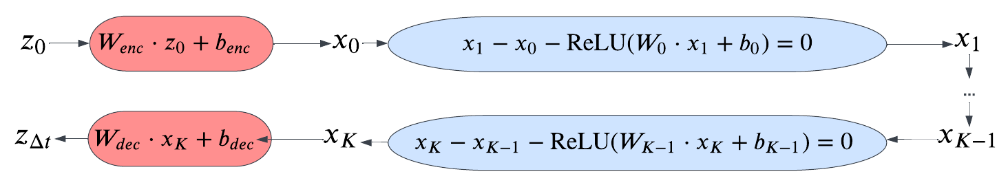
Figure 2: Implicit neural network architecture with K residual blocks.

6.2 Forecasting settings

As described in section 2.2, traditional methods forecast by using the output of the network at time $t$ to predict the dynamics at time $t+\Delta t$. Figure 3 illustrates this setting. However, the forecast can also be done within the latent space of the network. Figure 4 illustrates this different setting.

Figure 3: Traditional auto-regressive forecasting.

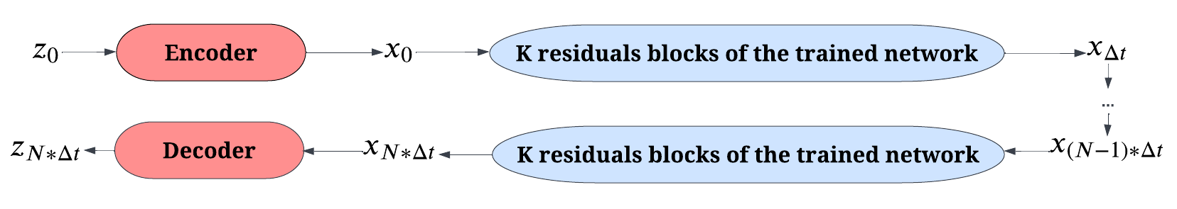
Figure 4: Latent-space auto-regressive forecasting.

7 Details on experiments

7.1 Baseline Methods

In addition to an Explicit ResNet with ReLU activation function and a FNO, we have two variants for the explicit ResNet method.

• an explicit ResNet tanh, with $R_{n}(x)=\tanh(W_{n}x+b_{n})$

• an explicit ResNet BN, with a ReLU activation function, and batch normalization at each hidden layer, to control the norm inside the network.

7.2 On training

The training details for each architecture on both equations are presented in the appendix in Table 7.3. For the Advection equation, 350 examples were generated for train, 150 other ones for validation/test and 50 for forecasting tests. For Burgers’ equation, 120 examples were generated for train, 30 other ones for validation/test and 50 for forecasting tests. Our experiments led to a few main training remarks.

Initialization

The networks are not really sensitive to the initialization. The only pitfall is to initialize with high values. Then the network doesn’t manage to converge as well as it could have. We initialize all networks with Xavier initialization with a gain of 1.

Learning rate scheduling

We used learning rate scheduling. It improves performance by a factor of 100. It is crucial to use it for our problems, and to choose carefully its parameter. We found that a linear scheduling with carefully chosen decay and step size works well. A special attention needs to be placed on the initial learning rate as well.

FNO architecture

For the FNO network, we chose 12 modes a width of 32 for the Advection equation and 16 modes and a width of 64 for Burgers’ equation, as was done in the original article.

7.3 Training parameters

The training remarks detailed previously in section 7.2 led to the choices showed in Table 7.3.

Table 2: Hyper-parameter choice for each architecture on the Advection equation and Burgers’ equation.

		Model	Xavier gain	Initial learning rate	Decay	Step size	Epochs
Advection		Explicit Res Net	1	0.05	0.95	10	2500
		Explicit Res Net BN	1	0.05	0.98	10	2500
		Explicit Res Tanh	1	0.05	0.95	10	2500
		FNO	1	0.005	0.98	10	2500
		Implicit ResNet (Ours)	1	0.01	0.9	10	1250
Burgers’		Explicit Res Net	1	0.05	0.95	10	2500
		Explicit Res Net BN	1	0.05	0.98	10	2500
		Explicit Res Tanh	1	0.05	0.95	10	2500
		FNO	1	0.005	0.96	10	2500
		Implicit ResNet (Ours)	1	0.01	0.98	10	1250

7.4 Ablation study

In order to better investigate this task, we conducted experiments with additional architectures. The results are shown in Table 7.4.

Table 3: Ablation study for the Advection equation and Burgers’ equation.

		Model	Train Error ($\times 10^{-4}$)	Test Error ($\times 10^{-4}$)	Forecast error at mid-range $T_{adv}=40\cdot\Delta t_{adv}$ $T_{bur}=150\cdot\Delta t_{bur}$	Forecast error at long-range $T_{adv}=400\cdot\Delta t_{adv}$ $T_{bur}=300\cdot\Delta t_{bur}$
Advection		Explicit Res Net	0.03 ± 0.01	0.09 ± 0.07	0.25 ± 0.33	$4.7\cdot 10^{31}$ ± $1.0\cdot 10^{32}$
		Explicit Res Net BN	1.01 ± 0.32	317 ± 20	$1.2\cdot 10^{24}$ ± $2.8\cdot 10^{24}$	$+\infty$
		Explicit Res Tanh	0.98 ± 0.1	14.0 ± 4.0	31.7 ± 70.5	$+\infty$
		FNO	0.04 ± 0.01	0.1 ± 0.08	0.03 ± 0.04	$4.7\cdot 10^{8}$ ± $1.0\cdot 10^{9}$
		Implicit ResNet (Ours)	14.0 ± 9.0	25.0 ± 27.0	27.4 ± 24	27.5 ± 24.2
Burgers’		Explicit Res Net	0.17 ± 0.03	0.90 ± 0.38	$2.77\cdot 10^{19}$ ± $6.2\cdot 10^{19}$	$+\infty$
		Explicit Res Net BN	0.51 ± 0.13	51.63 ± 34.89	$+\infty$	$+\infty$
		Explicit Res Tanh	0.84 ± 0.22	44.67 ± 11.58	$+\infty$	$+\infty$
		FNO	0.02 ± 0.002	0.03 ± 0.006	$5.31\cdot 10^{10}$ ± $11.2\cdot 10^{10}$	$+\infty$
		Implicit ResNet (Ours)	4.90 ± 0.64	7.91 ± 0.30	0.67 ± 0.43	0.66 ± 0.44

Table 4: Results of our approach compared to baselines on the Advection equation and Burgers’ equation. We calculate the means and standard deviations of relative error for each model based on 5 runs with different seeds. The mid-range time is 40 for the Advection equation and 0.075 for Burgers’ and the long range time is respectively 400 and 0.15. Recall that $\Delta t_{adv}=1$ and $\Delta t_{bur}=0.0005$. All relative errors are in percentages.

		Model	Test relative Error	Relative error at mid-range $T_{adv}=40\cdot\Delta t_{adv}$ $T_{bur}=150\cdot\Delta t_{bur}$	Relative error at long-range $T_{adv}=400\cdot\Delta t_{adv}$ $T_{bur}=300\cdot\Delta t_{bur}$
Advection		Explicit Res Net	0.5 ± 0.009	106.5 ± 66.0	$+\infty$
		FNO	1.1 ± 0.1	34.5 ± 19.0	$7.2\cdot 10^{5}$ ± $1.6\cdot 10^{6}$
		Implicit ResNet (Ours)	10.7 ± 4.2	1026.8 ± 346.7	1037.1 ± 347.9
Burgers’		Explicit Res Net	2.9 ± 0.3	$6.9\cdot 10^{10}$ ± $1.5\cdot 10^{11}$	$+\infty$
		FNO	0.6 ± 0.004	$3.6\cdot 10^{6}$ ± $8.0\cdot 10^{6}$	$+\infty$
		Implicit ResNet (Ours)	10.7 ± 0.3	277.7 ± 102.6	340.0 ± 129.9

References

- Ayed et al. [2019] I. Ayed, E. de Bézenac, A. Pajot, J. Brajard, and P. Gallinari. Learning dynamical systems from partial observations. arXiv preprint arXiv:1902.11136, 2019.
- Brandstetter et al. [2022] J. Brandstetter, D. Worrall, and M. Welling. Message passing neural pde solvers. arXiv preprint arXiv:2202.03376, 2022.
- Chen et al. [2018] R. T. Chen, Y. Rubanova, J. Bettencourt, and D. Duvenaud. Neural ordinary differential equations. arXiv preprint arXiv:1806.07366, 2018.
- El Ghaoui et al. [2019] L. El Ghaoui, F. Gu, B. Travacca, A. Askari, and A. Y. Tsai. Implicit deep learning. arXiv preprint arXiv:1908.06315, 2, 2019.
- Fotiadis et al. [2020] S. Fotiadis, E. Pignatelli, M. L. Valencia, C. Cantwell, A. Storkey, and A. A. Bharath. Comparing recurrent and convolutional neural networks for predicting wave propagation. arXiv preprint arXiv:2002.08981, 2020.
- Haber and Ruthotto [2017] E. Haber and L. Ruthotto. Stable architectures for deep neural networks. Inverse Problems, 34(1):014004, 2017.
- Haber et al. [2019] E. Haber, K. Lensink, E. Treister, and L. Ruthotto. Imexnet a forward stable deep neural network. In International Conference on Machine Learning, pages 2525–2534. PMLR, 2019.
- Horie and Mitsume [2022] M. Horie and N. Mitsume. Physics-embedded neural networks: E (n)-equivariant graph neural pde solvers. arXiv preprint arXiv:2205.11912, 2022.
- Kasim and Vinko [2020] M. F. Kasim and S. M. Vinko. xi-torch: differentiable scientific computing library. arXiv preprint arXiv:2010.01921, 2020.
- Kim et al. [2019] B. Kim, V. C. Azevedo, N. Thuerey, T. Kim, M. Gross, and B. Solenthaler. Deep fluids: A generative network for parameterized fluid simulations. In Computer Graphics Forum, volume 38, pages 59–70. Wiley Online Library, 2019.
- Li et al. [2020a] M. Li, L. He, and Z. Lin. Implicit euler skip connections: Enhancing adversarial robustness via numerical stability. In International Conference on Machine Learning, pages 5874–5883. PMLR, 2020a.
- Li et al. [2020b] Z. Li, N. Kovachki, K. Azizzadenesheli, B. Liu, K. Bhattacharya, A. Stuart, and A. Anandkumar. Fourier neural operator for parametric partial differential equations. arXiv preprint arXiv:2010.08895, 2020b.
- Lino et al. [2020] M. Lino, C. Cantwell, S. Fotiadis, E. Pignatelli, and A. Bharath. Simulating surface wave dynamics with convolutional networks. arXiv preprint arXiv:2012.00718, 2020.
- Nonnenmacher and Greenberg [2021] M. Nonnenmacher and D. S. Greenberg. Learning implicit pde integration with linear implicit layers. In The Symbiosis of Deep Learning and Differential Equations, 2021.
- Reshniak and Webster [2021] V. Reshniak and C. G. Webster. Robust learning with implicit residual networks. Machine Learning and Knowledge Extraction, 3(1):34–55, 2021.
- Shen et al. [2020] J. Shen, Z. Li, L. Yu, G.-S. Xia, and W. Yang. Implicit euler ode networks for single-image dehazing. In Proceedings of the IEEE/CVF Conference on Computer Vision and Pattern Recognition Workshops, pages 218–219, 2020.
- Sorteberg et al. [2019] W. E. Sorteberg, S. Garasto, C. C. Cantwell, and A. A. Bharath. Approximating the solution of surface wave propagation using deep neural networks. In INNS Big Data and Deep Learning conference, pages 246–256. Springer, 2019.
- van de Rotten and Lunel [2005] B. van de Rotten and S. V. Lunel. A limited memory broyden method to solve high-dimensional systems of nonlinear equations. In EQUADIFF 2003, pages 196–201. World Scientific, 2005.
- Wiewel et al. [2019] S. Wiewel, M. Becher, and N. Thuerey. Latent space physics: Towards learning the temporal evolution of fluid flow. In Computer graphics forum, volume 38, pages 71–82. Wiley Online Library, 2019.
- Zhang and Schaeffer [2020] L. Zhang and H. Schaeffer. Forward stability of resnet and its variants. Journal of Mathematical Imaging and Vision, 62(3):328–351, 2020.