Off-diagonal estimates for the helical maximal function

Abstract.

The optimal $L^{p}\to L^{q}$ mapping properties for the (local) helical maximal function are obtained, except for endpoints. The proof relies on tools from multilinear harmonic analysis and, in particular, a localised version of the Bennett–Carbery–Tao restriction theorem.

1. Introduction

1.1. Main results

Let $\gamma\colon I\to\mathbb{R}^{3}$ be a smooth curve, where $I:=[-1,1]$, which is non-degenerate in the sense that there is a constant $c_{0}>0$ such that

$$|\det(\gamma^{(1)}(s),\gamma^{(2)}(s),\gamma^{(3)}(s))|\geq c_{0}\qquad\textrm{for all $s\in I$.}$$ (1.1)

This is equivalent to saying that $\gamma$ has non-vanishing curvature and torsion. Prototypical examples are the helix $\gamma(s)=(\cos(2\pi s),\sin(2\pi s),s)$ or the moment curve $\gamma(s)=(s,s^{2}/2,s^{3}/6)$. Given $t>0$, consider the averaging operator

$$A_{t}f(x):=\int_{\mathbb{R}}f(x-t\gamma(s))\,\chi(s)\,\mathrm{d}s,$$

defined initially for Schwartz functions $f\in\mathcal{S}(\mathbb{R}^{3})$, where $\chi\in C^{\infty}(\mathbb{R})$ is a bump function supported on the interior of $I$. Furthermore, define the associated local maximal function

$$M_{\gamma}f(x):=\sup_{1\leq t\leq 2}|A_{t}f(x)|.$$

Here we are interested in determining the sharp range of $L^{p}\to L^{q}$ estimates for $M_{\gamma}$. To describe the results, let

$$\mathcal{T}:=\overline{\textrm{conv}\{(0,0),(1/3,1/3),(1/4,1/6)\}}\,\setminus\,\{(1/3,1/3)\},$$

so that $\mathcal{T}$ is a closed triangle (formed by the closed convex hull of three points) with one vertex removed. We let $\mathrm{int}(\mathcal{T})$ denote the interior of $\mathcal{T}$ and $\mathcal{L}$ denote the intersection of $\mathcal{T}$ with the diagonal: see Figure 1. Standard examples show that $M_{\gamma}$ fails to be $L^{p}\to L^{q}$ bounded whenever $(1/p,1/q)\notin\mathcal{T}$: see §9. The following theorem therefore characterises the type set of $M_{\gamma}$, up to endpoints.

Theorem 1.1.

For all $(1/p,1/q)\in\mathrm{int}(\mathcal{T})\cup\mathcal{L}$, there exists a constant $C_{\gamma,p,q}\geq 1$ such that the a priori estimate

$$\|M_{\gamma}f\|_{L^{q}(\mathbb{R}^{3})}\leq C_{\gamma,p,q}\|f\|_{L^{p}(\mathbb{R}^{3})}$$

holds for all $f\in\mathcal{S}(\mathbb{R}^{3})$.

For the diagonal case (that is, $(1/p,1/q)\in\mathcal{L}$), the sharp range of estimates was established in [2] and [18], building on earlier work of [21]. Hence, our main result is to push the range of boundedness to the region $\mathrm{int}(\mathcal{T})$. As a consequence of Theorem 1.1 (or, more precisely, Theorem 3.1 below) and [4, Theorem 1.4], $(p,q^{\prime})$-sparse bounds for the full maximal operator $M_{\gamma}^{\mathrm{full}}f(x):=\sup_{t>0}|A_{t}f(x)|$ follow for $(1/p,1/q)\in\mathrm{int}(\mathcal{T})\cup\mathcal{L}$. We omit the details and refer to [4] for the precise statements.

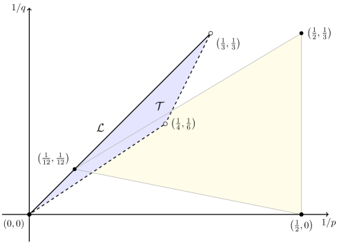
Figure 1. The known range of $L^{p}\to L^{q}$ boundedness for the helical maximal function. In [2] and [18], boundedness was shown on the half-open line segment $\mathcal{L}$ connecting $(0,0)$ and $(1/3,1/3)$. By Theorem 1.1, the operator is bounded whenever $(1/p,1/q)\in\mathrm{int}(\mathcal{T})$, the interior of the triangle with vertices $(0,0)$, $(1/3,1/3)$ and $(1/4,1/6)$. Frequency localised estimates are obtained at the critical vertex $(1/4,1/6)$ by interpolating multilinear inequalities at $(1/2,1/3)$, $(1/12,1/12)$ and $(1/2,0)$; see §3.5 below.

1.2. Methodology

Here we provide a brief overview of the ingredients of the proof of Theorem 1.1 and the novel features of the argument. For fixed $t$, the averaging operators $A_{t}$ correspond to convolution with an appropriate measure $\mu_{t}$ on the $t$-dilate of $\gamma$. It is therefore natural to study these objects via the Fourier transform, which leads us to consider the multiplier

$$\hat{\mu}_{t}(\xi)=\int_{\mathbb{R}}e^{-it\langle\gamma(s),\xi\rangle}\chi(s)\,\mathrm{d}s.$$

Stationary phase can be used to compute the decay rate of this function in different directions in the frequency space. This involves analysing the vanishing of $s$-derivatives of the phase function $\phi(\xi,s):=\langle\gamma(s),\xi\rangle$. Following earlier work on the circular maximal function [20], it is also useful to study the Fourier transform of $A_{t}f(x)$ in both the $x$ and the $t$ variables. This leads us to consider the $4$-dimensional $(\xi,\tau)$ frequency space.

Broadly speaking, this approach was taken in both works [18] and [2] to study the $L^{p}\to L^{p}$ mapping properties of $M_{\gamma}$. However, these papers focused on different geometrical aspects of the problem. In very rough terms, the analysis of [18] centres around a $3$-dimensional cone $\Gamma_{3}$ in $(\xi,\tau)$-space arising from the equations $\partial_{s}\phi(\xi,s)=0$, $\tau=\phi(\xi,s)$. On the other hand, the analysis of [2] centres around a $2$-dimensional cone $\Gamma_{2}$ in the $(\xi,\tau)$-space arising from the system of equations $\partial_{s}\phi(\xi,s)=\partial_{s}^{2}\phi(\xi,s)=0$, $\tau=\phi(\xi,s)$.

It seems difficult to obtain almost optimal $L^{p}\to L^{q}$ estimates using either the approach of [18] or of [2] in isolation; rather, it appears necessary to incorporate both geometries into the analysis. In order to do this, we apply a recent observation of Bejenaru [1], which provides a localised variant of the Bennett–Carbery–Tao multilinear restriction theorem [7]. We describe the relevant setup in detail in §2 below; moreover, in the appendix we relate the required localised estimates to the theory of Kakeya–Brascamp–Lieb inequalities from [6]. The local multilinear restriction estimate allows us to work simultaneously with the $\Gamma_{2}$ and $\Gamma_{3}$ geometries, by considering the embedded cone $\Gamma_{2}$ as a localised portion of $\Gamma_{3}$. See Proposition 3.5 below.

On the other hand, the geometries of both $\Gamma_{2}$ and $\Gamma_{3}$ were previously exploited in a non-trivial manner in [19] and [3] using the decoupling inequalities from [10]. This approach is inspired by earlier work of Pramanik–Seeger [21]. Decoupling is effective for proving $L^{p}\to L^{p}$ bounds for large $p$; here it is used to provide a counterpoint for interpolation with the estimates obtained via local multilinear restriction. See Proposition 3.6 below.

1.3. Notational conventions

Throughout the paper, $I$ denotes the interval $[-1,1]$.

We let $\widehat{\mathbb{R}}$ denote the frequency domain, which is the Pontryagin dual group of $\mathbb{R}$ understood here as simply a copy of $\mathbb{R}$. Given $f\in L^{1}(\mathbb{R}^{d})$ and $g\in L^{1}(\widehat{\mathbb{R}}^{d})$ we define the Fourier transform and inverse Fourier transform by

$$\hat{f}(\xi):=\int_{\mathbb{R}^{d}}e^{-i\langle x,\xi\rangle}f(x)\,\mathrm{d}x\quad\textrm{and}\quad\check{g}(x):=\frac{1}{(2\pi)^{d}}\int_{\widehat{\mathbb{R}}^{d}}e^{i\langle x,\xi\rangle}g(\xi)\,\mathrm{d}\xi,$$

respectively. For $m\in L^{\infty}(\widehat{\mathbb{R}}^{d})$ we define the multiplier operator $m(D)$ which acts initially on Schwartz functions by

$$m(D)f(x):=\frac{1}{(2\pi)^{d}}\int_{\widehat{\mathbb{R}}^{d}}e^{i\langle x,\xi\rangle}m(\xi)\hat{f}(\xi)\,\mathrm{d}\xi.$$

Given a list of objects $L$ and real numbers $A$, $B\geq 0$, we write $A\lesssim_{L}B$ or $B\gtrsim_{L}A$ to indicate $A\leq C_{L}B$ for some constant $C_{L}$ which depends only items in the list $L$ and our choice of underlying non-degenerate curve $\gamma$. We write $A\sim_{L}B$ to indicate $A\lesssim_{L}B$ and $B\lesssim_{L}A$.

1.4. Organisation of the paper

• In §2 we present the key localised trilinear restriction estimate.

• In §3 we describe a reduction of Theorem 1.1 to three local-smoothing-type estimates: trilinear $L^{2}\to L^{3}$, linear $L^{12}\to L^{12}$ and trivial $L^{2}\to L^{\infty}$.

• In §4 we describe the basic properties of our operators and prove the trivial $L^{2}\to L^{\infty}$ estimate.

• In §5 we prove the trilinear $L^{2}\rightarrow L^{3}$ estimate using the trilinear restriction theorem from §2.

• In §6 we prove the linear $L^{12}\rightarrow L^{12}$ estimate using decoupling.

• In §7 we bound a non-degenerate portion of the operator.

• In §8 we carry out the reduction described in §3 and thereby bound the remaining degenerate portion of the operator.

• In §9 we demonstrate the sharpness of the range $\mathcal{T}$.

• Finally, in Appendix A we present a proof of the localised trilinear restriction theorem from §2.

Acknowledgements

The first and third authors would like to thank Shaoming Guo and Andreas Seeger for discussions related to the topic of this paper over the years.

2. Localised trilinear restriction

The key ingredient in the proof of Theorem 1.1 is a localised trilinear Fourier restriction estimate. Here we describe the particular setup for our problem. As in [18], it is necessary to work with functions with a limited degree of regularity.

Definition 2.1.

Let $0<\alpha\leq 1$ and $U\subseteq\mathbb{R}^{d}$ be an open set. We say a function $Q\colon U\to\mathbb{R}$ is of class $C^{1,\alpha}(U)$ if it is continuously differentiable on $U$ and, moreover, the partial derivatives satisfy the $\alpha$-Hölder condition

$$\sup_{\begin{subarray}{c}\xi_{1},\xi_{2}\in U\\ \xi_{1}\neq\xi_{2}\end{subarray}}\frac{|\nabla Q(\xi_{1})-\nabla Q(\xi_{2})|}{|\xi_{1}-\xi_{2}|^{\alpha}}<\infty.$$

Consider an ensemble $\mathbf{Q}=(Q_{1},Q_{2},Q_{3})$ of maps $Q_{j}\colon U_{j}\to\mathbb{R}$ of class $C^{1,1/2}(U_{j})$ where $U_{j}\subseteq\widehat{\mathbb{R}}^{3}$ is an open domain for $1\leq j\leq 3$. The graphs

$$\Sigma_{j}:=\{(\xi,Q_{j}(\xi)):\xi\in U_{j}\}$$

are hypersurfaces in $\widehat{\mathbb{R}}^{4}$, with some limited regularity. Each $\Sigma_{j}$ has a Gauss map given by

$$\nu_{j}\colon U_{j}\to S^{3},\qquad\nu_{j}(\xi):=\frac{1}{(1+|\nabla Q_{j}(\xi)|^{2})^{1/2}}\begin{pmatrix}-\nabla Q_{j}(\xi)\\ 1\end{pmatrix}\qquad\textrm{for all $\xi\in U_{j}$.}$$

We further fix a smooth function $u\colon U_{3}\to\mathbb{R}$ satisfying $|\nabla u(\xi)|>c_{0}>0$ for all $\xi\in U_{3}$. This implicitly defines a smooth surface $Z_{3}:=\{\xi\in\widehat{\mathbb{R}}^{3}:u(\xi)=0\}$, which we lift to

$$\Sigma_{3}^{\prime}:=\{(\xi,Q_{3}(\xi)):\xi\in Z_{3}\}.$$

Thus, $\Sigma_{3}^{\prime}$ is a codimension 1 submanifold of $\Sigma_{3}$, which is embedded in $\widehat{\mathbb{R}}^{4}$. Defining

$$\nu_{3}^{\prime}\colon Z_{3}\to S^{3},\quad\nu_{3}^{\prime}(\xi):=\frac{1}{|\nabla u(\xi)|}\begin{pmatrix}\nabla u(\xi)\\ 0\end{pmatrix}\qquad\textrm{for all $\xi\in Z_{3}$,}$$

it follows that $\{\nu_{3}(\xi),\nu_{3}^{\prime}(\xi)\}$ forms a basis of the normal space to $\Sigma_{3}^{\prime}$ at $(\xi,Q_{3}(\xi))$ for all $\xi\in Z_{3}$.

We now fix $a_{j}\in C_{c}(U_{j})$ with $\|a_{j}\|_{L^{\infty}(U_{j})}\leq 1$ for $1\leq j\leq 3$ and we assume the transversality hypothesis

$$\bigg{|}\det\begin{pmatrix}\nabla Q_{1}(\xi_{1})&\nabla Q_{2}(\xi_{2})&\nabla Q_{3}(\xi_{3})&\nabla u(\xi_{3})\\ 1&1&1&0\end{pmatrix}\bigg{|}>c_{\mathrm{trans}}>0$$ (2.1)

for all $\xi_{j}\in\mathrm{supp}\,a_{j}$, $1\leq j\leq 3$. Furthermore, given $0<\mu<1$, we assume the additional localisation hypothesis

$$|u(\xi)|<\mu\qquad\textrm{for all $\xi\in\mathrm{supp}\,a_{3}$.}$$ (2.2)

Finally, we define the extension operators

$$E_{j}f(x,t):=\int_{\widehat{\mathbb{R}}^{3}}e^{i(\langle x,\xi\rangle+tQ_{j}(\xi))}a_{j}(\xi)f(\xi)\,\mathrm{d}\xi\qquad\textrm{for $f\in L^{1}(U_{j})$, $1\leq j\leq 3$.}$$

The key localised trilinear estimate is as follows.

Theorem 2.2 (Localised trilinear restriction).

With the above setup, for all $\varepsilon>0$ and all $R\geq 1$ we have

$$\Big{\|}\prod_{j=1}^{3}|E_{j}f_{j}|^{1/3}\Big{\|}_{L^{3}(B(0,R))}\lesssim_{\mathbf{Q},\varepsilon}R^{\varepsilon}\mu^{1/6}\prod_{j=1}^{3}\|f_{j}\|_{L^{2}(U_{j})}^{1/3}$$

for all $f_{j}\in L^{1}(U_{j})$, $1\leq j\leq 3$.

Here the implied constant depends on the choice of maps $Q_{j}$ and, in particular, the lower bound in (2.1), but is (crucially) independent of the choice of parameter $\mu$ in (2.2) and the choice of scale $R$.

If we consider smooth hypersurfaces rather than the $C^{1,1/2}$ class, then Theorem 2.2 is a special case of [1, Theorem 1.3]. We expect that the arguments of [1] can be generalised to treat $C^{1,\alpha}$ regularity for all $\alpha>0$. However, in Appendix A we observe that Theorem 2.2 is a rather direct consequence of the Kakeya–Brascamp–Lieb inequalities from [6] (see also [24, 25]).

3. Initial reductions

3.1. Local smoothing estimates

The multipliers of interest are of the following form. For $I:=[-1,1]$, let $\gamma\colon I\to\mathbb{R}^{3}$ be a smooth curve and fix $\rho\in C^{\infty}_{c}(\mathbb{R})$ supported in the interior $[1/2,4]$. Given a symbol $a\in C^{\infty}(\widehat{\mathbb{R}}^{3}\setminus\{0\}\times\mathbb{R}\times\mathbb{R})$, we define

$$m_{\gamma}[a](\xi;t)\equiv m[a](\xi;t):=\int_{\mathbb{R}}e^{-it\langle\gamma(s),\xi\rangle}a(\xi;t;s)\psi_{I}(s)\rho(t)\,\mathrm{d}s,$$ (3.1)

for some $\psi_{I}\in C^{\infty}(\mathbb{R})$ with support lying in $I$. Fix $\eta\in C^{\infty}_{c}(\mathbb{R})$ non-negative, even and such that

$$\eta(r)=1\quad\textrm{if $r\in I$}\quad\textrm{and}\quad\mathrm{supp}\,\eta\subseteq[-2,2]$$

and define $\beta$, $\beta^{k}\in C^{\infty}_{c}(\mathbb{R})$ by

$$\beta(r):=\eta(r)-\eta(2r)\quad\textrm{and}\quad\beta^{k}(r):=\beta(2^{-k}r)\qquad\textrm{for all $k\in\mathbb{Z}$.}$$ (3.2)

By an abuse of notation, we also write $\eta(\xi):=\eta(|\xi|)$ and $\beta^{k}(\xi):=\beta^{k}(|\xi|)$ for $\xi\in\widehat{\mathbb{R}}^{3}$.

For $a\in C^{\infty}(\widehat{\mathbb{R}}^{3}\setminus\{0\}\times\mathbb{R}\times\mathbb{R})$ as above, we form a dyadic decomposition by writing

$$a=\sum_{k=0}^{\infty}a_{k}\qquad\textrm{where}\qquad a_{k}(\xi;t;s):=\left\{\begin{array}[]{ll}a(\xi;t;s)\,\beta^{k}(\xi)&\textrm{for $k\geq 1$}\\ a(\xi;t;s)\,\eta(\xi)&\textrm{for $k=0$}\end{array}\right..$$ (3.3)

With the above definitions, our main result is as follows.

Theorem 3.1 ($L^{p}\to L^{q}$ local smoothing).

Let $\gamma:I\to\mathbb{R}^{3}$ be a smooth curve and suppose $a\in C^{\infty}(\widehat{\mathbb{R}}^{3}\setminus\{0\}\times\mathbb{R}\times\mathbb{R})$ satisfies the symbol condition

$$|\partial_{\xi}^{\alpha}\partial_{t}^{i}\partial_{s}^{j}a(\xi;t;s)|\lesssim_{\alpha,i,j}|\xi|^{-|\alpha|}\qquad\textrm{for all $\alpha\in\mathbb{N}_{0}^{3}$ and $i$, $j\in\mathbb{N}_{0}$}$$ (3.4)

and that

$$\sum_{j=1}^{3}|\langle\gamma^{(j)}(s),\xi\rangle|\gtrsim|\xi|\qquad\text{ for all $(\xi;s)\in\mathrm{supp}_{\xi}\,a\times I$}.$$ (3.5)

Then for all $(1/p,1/q)\in\mathrm{int}(\mathcal{T})$ there exists some $\varepsilon(p,q)>0$ such that

$$\Big{(}\int_{1}^{2}\|m[a_{k}](D;t)f\|_{L^{q}(\mathbb{R}^{3})}^{q}\,\mathrm{d}t\Big{)}^{1/q}\lesssim_{p,q}2^{-k/q-\varepsilon(p,q)k}\|f\|_{L^{p}(\mathbb{R}^{3})}$$

holds for all $k\in\mathbb{N}_{0}$, where $a_{k}$ is defined as in (3.3).

The desired maximal bound follows from Theorem 3.1 using a standard Sobolev embedding argument; we omit the details but refer the reader to [23, Chapter XI, §3], [21, §6] or [2, §2] for similar arguments.

By results of [2], Theorem 3.1 is known to hold along the diagonal line $\mathcal{L}$. By interpolation, it therefore suffices to prove an estimate at the critical vertex $(1/4,1/6)$ in the Riesz diagram (see Figure 1).

Proposition 3.2.

Under the hypotheses of Theorem 3.1, for $k\in\mathbb{N}_{0}$ and all $\varepsilon>0$, we have

$$\Big{(}\int_{1}^{2}\|m[a_{k}](D;t)f\|_{L^{6}(\mathbb{R}^{3})}^{6}\,\mathrm{d}t\Big{)}^{1/6}\lesssim_{\varepsilon}2^{-k/6+\varepsilon k}\|f\|_{L^{4}(\mathbb{R}^{3})}.$$ (3.6)

By the preceding discussion, our main theorem follows from Proposition 3.2. Henceforth, we focus on the proof of this critical estimate.

3.2. Trilinear reduction

If the hypothesis (3.5) is strengthened to

$$|\langle\gamma^{\prime}(s),\xi\rangle|+|\langle\gamma^{\prime\prime}(s),\xi\rangle|\gtrsim|\xi|\qquad\textrm{for all $(\xi;s)\in\mathrm{supp}_{\xi}\,a\times I$,}$$ (3.7)

then one can deduce the critical estimate (3.6) as a consequence of known local smoothing inequalities from [21] (see Theorem 6.8 below) and the Stein–Tomas Fourier restriction inequality. Given a small number $0<\delta<1$ and $k\in\mathbb{N}$, we perform this analysis on the symbols

$$a_{k,0}(\xi;t;s):=a_{k}(\xi;t;s)\big{(}1-\eta(2^{-k}\delta^{-20}G_{2}(s;\xi))\big{)}$$ (3.8)

where $G_{2}(s;\xi):=\sum_{j=1}^{2}|\langle\gamma^{(j)}(s),\xi\rangle|$; note that $a_{k,0}$ satisfies (3.7) with an implicit constant depending on $\delta$. We discuss this case in detail in §7.

The main difficulty is then to get to grips with the degenerate portion of the multiplier. For the above choice of $0<\delta<1$, this corresponds to the condition

$$|\langle\gamma^{\prime}(s),\xi\rangle|+|\langle\gamma^{\prime\prime}(s),\xi\rangle|\lesssim\delta^{20}|\xi|\qquad\textrm{for all $(\xi;s)\in\mathrm{supp}_{\xi}\,a\times I$;}$$ (3.9)

note that this is satisfied on the support of $\mathfrak{a}_{k}:=a_{k}-a_{k,0}$. To control the degenerate part, we work with a trilinear variant of Proposition 3.2, from which we deduce the corresponding linear estimate (3.6) via a standard application of the broad-narrow method from [11] (see also [16]).

To describe the trilinear setup, we introduce some notation. For $0<\delta<1$ as above, let $\mathfrak{J}(\delta)$ denote a covering of $I$ by essentially disjoint intervals of length $\delta$. Let $\mathfrak{J}^{3,\mathrm{sep}}(\delta)$ denote the collection of all triples $\mathbf{J}=\{J_{1},J_{2},J_{3}\}\subset\mathfrak{J}(\delta)$ which satisfy the separation condition $\mathrm{dist}(J_{i},J_{j})\geq 10\delta$ for $1\leq i<j\leq 3$. Given a bounded interval $J\subseteq\mathbb{R}$, we let $\psi_{J}\in C^{\infty}_{c}(\mathbb{R})$ satisfy $\mathrm{supp}\,\psi_{J}\subseteq J$ and $|\partial^{N}_{s}\psi_{J}(s)|\lesssim_{N}|J|^{-N}$ for all $N\in\mathbb{N}$. Similarly to (3.1), given a symbol $a\in C^{\infty}(\widehat{\mathbb{R}}^{3}\setminus\{0\}\times\mathbb{R}\times\mathbb{R})$, we define the multipliers adapted to an interval $J\in\mathfrak{J}(\delta)$ by

$$m^{J}_{\gamma}[a](\xi;t)\equiv m^{J}[a](\xi;t):=\int_{\mathbb{R}}e^{-it\langle\gamma(s),\xi\rangle}a(\xi;t;s)\psi_{J}(s)\rho(t)\,\mathrm{d}s.$$

With this setup, we prove the following estimate.

Proposition 3.3 ($L^{4}\to L^{6}$ trilinear local smoothing).

Let $k\in\mathbb{N}_{0}$, $\varepsilon>0$ and $\delta>0$. Under the hypotheses of Theorem 3.1 and further assuming (3.9), we have

$$\Big{(}\int_{1}^{2}\Big{\|}\prod_{J\in\mathbf{J}}|m^{J}[a_{k}](D;t)f_{J}|^{1/3}\Big{\|}_{L^{6}(\mathbb{R}^{3})}^{6}\,\mathrm{d}t\Big{)}^{1/6}\lesssim_{\varepsilon}\delta^{-O(1)}2^{-k/6+\varepsilon k}\prod_{J\in\mathbf{J}}\|f_{J}\|_{L^{4}(\mathbb{R}^{3})}^{1/3}$$

whenever $\mathbf{J}\in\mathfrak{J}^{3,\mathrm{sep}}(\delta)$ and $f_{J}\in\mathcal{S}(\mathbb{R}^{3})$ for $J\in\mathbf{J}$.

Here we use the notation $O(1)$ to denote an unspecified absolute constant. In applications, we work with relatively large values of $\delta$ (namely, $\delta\sim_{\varepsilon}1$) and accordingly there is no need to precisely track the $\delta$ dependence. We will also assume without loss of generality that $0<\delta<c$ where $c>0$ is a small absolute constant, chosen to satisfy the forthcoming requirements of the argument, and $k$ is sufficiently large depending on $\delta^{-1}$.

As mentioned above, the (ostensibly weaker) trilinear estimate in Proposition 3.3 implies the linear estimate in Proposition 3.2 (under the additional assumption (3.9)) using a variant of the procedure introduced in [11]. We postpone the details of this reduction to §8 below.

3.3. Reduction to perturbations of the moment curve

At small scales, any non-degenerate curve can be thought of as a perturbation of an affine image of the moment curve $\gamma_{\circ}(s):=(s,s^{2}/2,s^{3}/6)$. We refer to [2, §4] for details (which involve the affine rescalings described in §4.2 below), and just record here that it suffices to consider curves in the class $\mathfrak{G}(\delta_{0})$ defined below for $0<\delta_{0}<1$ sufficiently small.

Definition 3.4.

Given $0<\delta_{0}<1$ and $M\in\mathbb{N}$, let $\mathfrak{G}(\delta_{0},M)$ denote the class of all smooth curves $\gamma\colon I\to\mathbb{R}^{3}$ that satisfy the following conditions:

1. $\gamma(0)=0$ and $\gamma^{(j)}(0)=\vec{e}_{j}$ for $1\leq j\leq 3$;

2. $\|\gamma-\gamma_{\circ}\|_{C^{M}(I)}\leq\delta_{0}$ for all $0\leq j\leq M$.

Here $\vec{e}_{j}$ denotes the $j$th standard Euclidean basis vector and

$$\|\gamma\|_{C^{M}(I)}:=\max_{1\leq j\leq M}\sup_{s\in I}|\gamma^{(j)}(s)|\qquad\textrm{for all $\gamma\in C^{M}(I;\mathbb{R}^{3})$.}$$

If $M=4$, then we will simply write $\mathfrak{G}(\delta_{0})$ for $\mathfrak{G}(\delta_{0},4)$

Henceforth we will always assume that $\gamma\in\mathfrak{G}(\delta_{0})$ for $\delta_{0}:=10^{-10}$.

3.4. Microlocal decomposition

Under the assumption (3.9), the non-degeneracy condition (1.1) ensures that

$$|\langle\gamma^{\prime\prime\prime}(s),\xi\rangle|\gtrsim|\xi|\quad\text{ for all $(\xi;t;s)\in\mathrm{supp}\,a$;}$$ (3.10)

indeed, for $\gamma\in\mathfrak{G}(\delta_{0})$ this condition holds for all $(\xi;t;s)\in\mathrm{supp}_{\xi}\,a\times\mathbb{R}\times I$. We can then assume that $s\mapsto\langle\gamma^{\prime\prime\prime}(s),\xi\rangle$ has constant sign and henceforth we assume that $\xi_{3}>0$. Following [2, §6], let $\theta_{2}\colon\mathrm{supp}_{\xi}\,a\to I$ be the smooth mapping such that

$$\langle\gamma^{\prime\prime}\circ\theta_{2}(\xi),\xi\rangle=0\qquad\textrm{for all $\xi\in\mathrm{supp}_{\xi}\,a$.}$$

It is clear that $\theta_{2}$ is homogeneous of degree 0. Let

$$u(\xi):=\langle\gamma^{\prime}\circ\theta_{2}(\xi),\xi\rangle\qquad\textrm{for all $\xi\in\mathrm{supp}_{\xi}\,a$.}$$ (3.11)

Since (3.10) is satisfied on the support of each

$$\mathfrak{a}_{k}:=a_{k}-a_{k,0},$$ (3.12)

we decompose each of these pieces with respect to the size of $|u(\xi)|$. Given $\varepsilon>0$ and $0<\delta<1$, we write

$$a_{k}=a_{k,0}+\sum_{\ell\in\Lambda(k)}a_{k,\ell}+a_{k,k/3}$$ (3.13)

where $a_{k,0}$ is as in (3.8) and

$$a_{k,\ell}(\xi;t;s):=\left\{\begin{array}[]{ll}\displaystyle\mathfrak{a}_{k}(\xi;t;s)\,\beta\big{(}2^{-k+2\ell}u(\xi)\big{)}&\textrm{if $\ell\in\Lambda(k)$,}\\[8.0pt] \displaystyle\mathfrak{a}_{k}(\xi;t;s)\,\eta\big{(}2^{-k+2\lfloor(1-2\varepsilon)k/3\rfloor}u(\xi)\big{)}&\textrm{if $\ell=k/3$}\end{array}\right.$$ (3.14)

for

$$\Lambda(k):=\{\,\ell\in\mathbb{N}:\lceil\log_{2}(\delta^{-8})\rceil<\ell<\left\lfloor(1-2\varepsilon)k/3\right\rfloor\,\}.$$ (3.15)

Here we assume that $k$ is large enough so that the decomposition (3.13) makes sense; note that Theorem 3.1 trivially holds for small values of $k$. In particular, we concern ourselves with $k\in\mathbb{N}$ satisfying $k\geq 4\log_{2}(\delta^{-8})$. In the definition (3.15), for any $x\in\mathbb{R}$, we let $\lfloor x\rfloor$ denote the largest integer less or equal than $x$ and $\lceil x\rceil$ denote the smallest integer greater or equal than $x$. It will also be useful to introduce the notation

$$\overline{\Lambda}(k):=\Lambda(k)\cup\{k/3\}.$$

Note that the indexing set $\Lambda(k)$ depends on the chosen $\delta$ and $\varepsilon$, but we do not record this dependence for notational convenience. We also note that here the function $\beta$ should be defined slightly differently compared with (3.2); in particular, here $\beta(r):=\eta(2^{-2}r)-\eta(r)$ (we ignore this minor change in the notation).

As mentioned in §3.2, for the extreme case $\ell=0$ we have the non-degeneracy condition (3.7) (with an implied constant depending on $\delta$). This situation is easy to handle using known estimates: see §7 below. On the other hand, for $\ell\in\overline{\Lambda}(k)$, the multipliers $m[a_{k,\ell}]$ are degenerate in the sense that (3.9) now holds. A key aspect of this decomposition is that for $\ell\in\Lambda(k)$, Taylor series expansion shows that

$$|\langle\gamma^{\prime}(s),\xi\rangle|+2^{-\ell}|\langle\gamma^{\prime\prime}(s),\xi\rangle|\gtrsim 2^{k-2\ell}\qquad\textrm{for all $(\xi,s)\in\mathrm{supp}\,a_{k,\ell}(\,\cdot\,;t;\,\cdot\,)$;}$$ (3.16)

see, for example [3, (5.15)] for a detailed derivation. The weak non-degeneracy condition (3.16) will allow for improved estimates depending on the value of $\ell$. Bounding these pieces, and the piece for $\ell=k/3$, is the difficult part of the argument and is the focus of §§5–6 below.

3.5. Microlocalised estimates

Throughout this section we work under the hypotheses of Theorem 3.1 and, in addition, assume (3.9) holds for a specified value of $\delta$. That is, we let $\gamma:I\to\mathbb{R}^{3}$ be a smooth curve and suppose $a\in C^{\infty}(\widehat{\mathbb{R}}^{3}\setminus\{0\}\times\mathbb{R}\times\mathbb{R})$ satisfies (3.4), (3.5) and (3.9). Furthermore, we define the symbols $a_{k,\ell}$ as in (3.14).

The key ingredient in the proof of Proposition 3.3 is a trilinear estimate for the multipliers associated to the localised symbols $a_{k,\ell}$. To describe this result, we work with a triple of integers $\ell_{\mathbf{J}}=(\ell_{J})_{J\in\mathbf{J}}$ indexed by $\mathbf{J}\in\mathfrak{J}^{3,\mathrm{sep}}(\delta)$ and write $|\ell_{\mathbf{J}}|:=\sum_{J\in\mathbf{J}}\ell_{J}$.

Proposition 3.5 ($L^{2}\to L^{3}$ trilinear local smoothing).

For $k\in\mathbb{N}$, $\varepsilon>0$ and $0<\delta<1$, we have

$$\Big{(}\int_{1}^{2}\Big{\|}\prod_{J\in\mathbf{J}}|m^{J}[a_{k,\ell_{J}}](D;t)f_{J}|^{1/3}\Big{\|}_{L^{3}(\mathbb{R}^{3})}^{3}\,\mathrm{d}t\Big{)}^{1/3}\lesssim_{\varepsilon}\delta^{-O(1)}2^{-k/3+|\ell_{\mathbf{J}}|/18+\varepsilon k}\prod_{j=1}^{3}\|f_{J}\|_{L^{2}(\mathbb{R}^{3})}^{1/3}$$

whenever $\mathbf{J}\in\mathfrak{J}^{3,\mathrm{sep}}(\delta)$, $\ell_{\mathbf{J}}=(\ell_{J})_{J\in\mathbf{J}}$ with $\ell_{J}\in\overline{\Lambda}(k)$ and $f_{J}\in\mathcal{S}(\mathbb{R}^{3})$ for $J\in\mathbf{J}$.

Proposition 3.5 is a fairly direct consequence of Theorem 2.2; we describe the proof in §5 below. To deduce the critical $L^{4}\to L^{6}$ estimate stated in Proposition 3.3, we interpolate Proposition 3.5 with the following linear inequalities.

Proposition 3.6 ($L^{12}\to L^{12}$ local smoothing).

For $k\in\mathbb{N}$, $\varepsilon>0$, $0<\delta<1$ and $\ell\in\overline{\Lambda}(k)$, we have

$$\Big{(}\int_{1}^{2}\|m[a_{k,\ell}](D;t)f\|_{L^{12}(\mathbb{R}^{3})}^{12}\,\mathrm{d}t\Big{)}^{1/12}\lesssim_{\varepsilon}2^{-k/6-\ell/12+\varepsilon k}\|f\|_{L^{12}(\mathbb{R}^{3})}.$$

Lemma 3.7 ($L^{2}\to L^{\infty}$ estimate).

For $k\in\mathbb{N}$, $\varepsilon>0$, $0<\delta<1$ and $\ell\in\overline{\Lambda}(k)$, we have

$$\sup_{1\leq t\leq 2}\|m[a_{k,\ell}](D;t)f\|_{L^{\infty}(\mathbb{R}^{3})}\lesssim 2^{k-\ell/2}\|f\|_{L^{2}(\mathbb{R}^{3})}.$$

We remark that $0<\delta<1$ plays no significant rôle in the proofs of Proposition 3.6 and Lemma 3.7 and it is used only to set up the underlying decomposition in the $a_{k,\ell}$. Similarly, $\varepsilon>0$ plays no significant rôle in Lemma 3.7.

Proposition 3.6 is a minor variant of estimates which have appeared in, for instance, [19] and [3]. The result is highly non-trivial, and relies on the $\ell^{p}$ decoupling inequality for the moment curve from [10]. We discuss the details in §6.

Lemma 3.7, on the other hand, is elementary. It follows from basic pointwise estimates for the multipliers $a_{k,\ell}$, obtained via stationary phase. We discuss the details in §4.1.

Given the preceding results, the key trilinear $L^{4}\to L^{6}$ local smoothing estimate is immediate.

Proof (of Proposition 3.3).

By multilinear Hölder’s inequality, Propositions 3.6 and 3.7 imply their trilinear counterparts. Since

$$\begin{pmatrix}\frac{1}{4}\\[3.0pt] \frac{1}{6}\end{pmatrix}=\frac{3}{5}\cdot\begin{pmatrix}\frac{1}{12}\\[3.0pt] \frac{1}{12}\end{pmatrix}+\frac{7}{20}\cdot\begin{pmatrix}\frac{1}{2}\\[3.0pt] \frac{1}{3}\end{pmatrix}+\frac{1}{20}\cdot\begin{pmatrix}\frac{1}{2}\\[3.0pt] 0\end{pmatrix},$$

interpolation of the three estimates immediately gives

$$\Big{(}\int_{1}^{2}\Big{\|}\prod_{J\in\mathbf{J}}|m^{J}[a_{k,\ell_{J}}](D;t)f|^{1/3}\Big{\|}_{L^{6}(\mathbb{R}^{3})}^{6}\,\mathrm{d}t\Big{)}^{1/6}\lesssim_{\varepsilon}\delta^{-O(1)}2^{-k/6-|\ell_{\mathbf{J}}|/180+\varepsilon k}\|f\|_{L^{4}(\mathbb{R}^{3})}$$

for $\ell_{\mathbf{J}}=(\ell_{J})_{J\in\mathbf{J}}$ with $0\leq\ell_{J}\leq k/3$; see Figure 1. Here we carry out the interpolation using a multilinear variant of the Riesz–Thorin theorem: see, for instance, [8, §4.4]. Using the geometric decay in $2^{-\ell_{J}}$ for each $J\in\mathbf{J}$, we sum these bounds to deduce the desired result. ∎

To prove Proposition 3.3, it therefore remains to establish Proposition 3.5, Proposition 3.6 and Lemma 3.7. We carry this out in §§4–6 below.

4. Basic properties of the multipliers

4.1. Elementary estimates for the multiplier

Using stationary phase arguments, we can immediately deduce Lemma 3.7.

Proof (of Lemma 3.7).

By the Cauchy–Schwarz inequality, we have the elementary inequality

$$\|m(D)f\|_{L^{\infty}(\mathbb{R}^{3})}\leq\|m\|_{L^{\infty}(\widehat{\mathbb{R}}^{3})}\big{|}\mathrm{supp}\,m\big{|}^{1/2}\|f\|_{L^{2}(\mathbb{R}^{3})}.$$

Fixing $t\in\mathbb{R}$, in view of the above it suffices to show

$$\|m[a_{k,\ell}](\,\cdot\,,t)\|_{\infty}\lesssim 2^{-(k-\ell)/2},\quad|\mathrm{supp}\,m[a_{k,\ell}](\,\cdot\,;t)|\lesssim 2^{3k-2\ell}.$$

Since $\nabla u(\xi)=\gamma^{\prime}\circ\theta_{2}(\xi)$ is bounded away from zero, the latter estimate is clear. On the other hand, the former estimate is a consequence of a simple stationary phase analysis. Indeed, for $\ell=k/3$ we apply van der Corput’s inequality with third order derivatives. For $\ell\in\Lambda(k)$, we apply van der Corput’s inequality with either first or second order derivatives, using the lower bound (3.16). For further details see, for example, [21, Lemma 3.3], [3, (5.15)] or Lemma 4.3 below. ∎

4.2. Scaling of the multiplier

Let $\sigma\in I$, $0<\lambda<1$ be such that $[\sigma-\lambda,\sigma+\lambda]\subseteq I$. Denote by $[\gamma]_{\sigma}$ the $3\times 3$ matrix

$$[\gamma]_{\sigma}:=\begin{bmatrix}\gamma^{(1)}(\sigma)&\gamma^{(2)}(\sigma)&\gamma^{(3)}(\sigma)\end{bmatrix},$$

where the vectors $\gamma^{(j)}(\sigma)$ are understood to be column vectors. Note that this matrix is invertible due to the non-degeneracy hypothesis (1.1). It is also convenient to let $[\gamma]_{\sigma,\lambda}$ denote the $3\times 3$ matrix

$$[\gamma]_{\sigma,\lambda}:=[\gamma]_{\sigma}\cdot D_{\lambda}$$ (4.1)

where $D_{\lambda}:=\text{diag}(\lambda,\lambda^{2},\lambda^{3})$ is the diagonal matrix with eigenvalues $\lambda$, $\lambda^{2},\lambda^{3}$. With this data, define the $(\sigma,\lambda)$-rescaling of $\gamma$ as the curve $\gamma_{\sigma,\lambda}\in C^{\infty}(I;\mathbb{R}^{3})$ given by

$$\gamma_{\sigma,\lambda}(s):=[\gamma]_{\sigma,\lambda}^{-1}\big{(}\gamma(\sigma+\lambda s)-\gamma(\sigma)\big{)}.$$ (4.2)

A simple computation shows

$$\det[\gamma_{\sigma,\lambda}]_{s}=\frac{\det\big{(}[\gamma]_{\sigma+\lambda s}\big{)}}{\det\big{(}[\gamma]_{\sigma}\big{)}},$$

and therefore $\gamma_{\sigma,\lambda}$ is also a non-degenerate curve. Furthermore, the rescaled curve satisfies the relations

$$\langle\gamma_{\sigma,\lambda}^{(j)}(s),\xi\rangle=\lambda^{j}\langle\gamma^{(j)}(\sigma+\lambda s),([\gamma]_{\sigma,\lambda})^{-\top}\xi\rangle\qquad\text{for all $j\geq 1$}.$$ (4.3)

Combining this with the fact that $\gamma_{\sigma,\lambda}$ is non-degenerate, we have

$$|\xi|\lesssim\sum_{j=1}^{3}|\langle\gamma_{\sigma,\lambda}^{(j)}(s),\xi\rangle|\lesssim\lambda^{3}|([\gamma]_{\sigma,\lambda})^{-\top}\xi|\lesssim|\xi|;$$ (4.4)

here the last inequality is a simple consequence of the definition (4.1).

Defining the rescaled symbol

$$a_{\sigma,\lambda}(\xi;t;s):=a(([\gamma]_{\sigma,\lambda})^{-\top}\xi;t;\sigma+\lambda s),$$ (4.5)

a change of variables immediately yields

$$m_{\gamma}[a](D;t)f(x)=\lambda\,m_{\gamma_{\sigma,\lambda}}[a_{\sigma,\lambda}](D;t)f_{\sigma,\lambda}(([\gamma]_{\sigma,\lambda})^{-1}(x-t\gamma(\sigma)))$$ (4.6)

where $f_{\sigma,\lambda}:=f\circ[\gamma]_{\sigma,\lambda}$. In particular, by scaling,

$$\|m_{\gamma}[a](D;\,\cdot\,)f\|_{L^{p}(\mathbb{R}^{3})\to L^{q}(\mathbb{R}^{3+1})}\lesssim\delta^{1+6(\frac{1}{q}-\frac{1}{p})}\|m_{\gamma_{\sigma,\lambda}}[a_{\sigma,\lambda}](D;\cdot)\|_{L^{p}(\mathbb{R}^{3})\to L^{q}(\mathbb{R}^{3+1})}.$$ (4.7)

Finally, we observe that if the original symbol satisfies the condition

$$|\partial_{\xi}^{\alpha}a(\xi;t;s)|\lesssim_{\alpha}|\xi|^{-|\alpha|}\qquad\textrm{for all $\alpha\in\mathbb{N}_{0}^{3}$},$$ (4.8)

then so too does the rescaled symbol $a_{\sigma,\lambda}$. Indeed, by the definitions (4.5) and (4.1), we have

$$|(\partial_{\xi}^{\alpha}a_{\sigma,\lambda})(\xi;t;s)|\lesssim_{\alpha}\lambda^{-3|\alpha|}|(\partial_{\xi}^{\alpha}a)(([\gamma]_{\sigma,\lambda})^{-\top}\xi;t;\sigma+\lambda s)|.$$

In view of the hypothesis (4.8) and (4.4), it follows that

$$|(\partial_{\xi}^{\alpha}a_{\sigma,\lambda})(\xi;t;s)|\lesssim_{\alpha}\lambda^{-3|\alpha|}\big{|}([\gamma]_{\sigma,\lambda})^{-\top}\xi\big{|}^{-|\alpha|}\lesssim_{\alpha}|\xi|^{-|\alpha|},$$

as required.

4.3. Critical points

We next describe the critical points of the phase function $s\mapsto\langle\gamma(s),\xi\rangle$ which, under the setup of §3.4, depend on the sign of the quantity $u(\xi)$ introduced in (3.11).

Lemma 4.1 ([2, Lemma 6.2]).

Let $\xi\in\mathrm{supp}_{\xi}\,a$ and consider the equation

$$\langle\gamma^{\prime}(s),\xi\rangle=0.$$ (4.9)

1. If $u(\xi)>0$, then the equation (4.9) has no solution on $I$.

2. If $u(\xi)=0$, then the equation (4.9) has only the solution $s=\theta_{2}(\xi)$ on $I$.

3. If $u(\xi)<0$, then the equation (4.9) has precisely two solutions on $I$.

Following [2, §6], we can use Lemma 4.1 to construct a (unique) pair of smooth mappings

$$\theta_{1}^{\pm}\colon\{\xi\in\mathrm{supp}_{\xi}\,a:u(\xi)<0\}\to I$$

with $\theta_{1}^{-}(\xi)\leq\theta_{1}^{+}(\xi)$ which satisfies

$$\langle\gamma^{\prime}\circ\theta_{1}^{\pm}(\xi),\xi\rangle=0\quad\text{ for all $\xi\in\mathrm{supp}_{\xi}\,a$ with $u(\xi)<0$.}$$

Define the functions

$$v^{\pm}(\xi):=\langle\gamma^{\prime\prime}\circ\theta_{1}^{\pm}(\xi),\xi\rangle\qquad\text{ for all $\xi\in\mathrm{supp}_{\xi}\,a$ with $u(\xi)<0$.}$$

Taylor expansion yields the following.

Lemma 4.2 ([2, Lemma 6.3]).

Let $\xi\in\mathrm{supp}_{\xi}\,a$ with $u(\xi)<0$. Then

$$\big{|}v^{\pm}\big{(}\tfrac{\xi}{|\xi|}\big{)}\big{|}\sim|\theta_{1}^{\pm}(\xi)-\theta_{2}(\xi)|\sim|\theta_{1}^{+}(\xi)-\theta_{1}^{-}(\xi)|\sim\big{|}u\big{(}\tfrac{\xi}{|\xi|}\big{)}\big{|}^{1/2}.$$

4.4. Stationary phase

We next use the approach in [18] and apply stationary phase to express the multipliers $m^{J}[a_{k,\ell}]$ as a product of a symbol and an oscillatory term. In what follows, we let

$$q_{2}(\xi):=\langle\gamma\circ\theta_{2}(\xi),\xi\rangle\qquad\textrm{and}\qquad q_{1}^{\pm}(\xi):=\langle\gamma\circ\theta_{1}^{\pm}(\xi),\xi\rangle$$

for any value of $\xi$ such that the expression is well-defined. Our analysis leads to various rapidly decreasing error terms. Given $R\geq 1$, we let $\mathrm{RapDec}(R)$ denote the class of functions $e\in C^{\infty}(\widehat{\mathbb{R}}^{3}\times\mathbb{R})$ which satisfy $|e(\xi;t)|\lesssim_{N}R^{-N}$ for all $N\in\mathbb{N}_{0}$.

Lemma 4.3.

Let $k\in\mathbb{N}$ and $J\in\mathfrak{J}(\delta)$.

1. For some $e_{k,k/3}\in\mathrm{RapDec}(2^{k})$, we may write

   $$m^{J}[a_{k,k/3}](\xi;t)=2^{-k/3}e^{-itq_{2}(\xi)}b^{J}_{k,k/3}(2^{-k}\xi;t)+e_{k,k/3}(\xi;t)$$ (4.10)

   where $b^{J}_{k,k/3}\in C^{\infty}(\mathbb{R}^{3+1})$ is supported in $B(0,10)$, satisfies $|u(\xi)|\lesssim 2^{-2k/3+4\varepsilon k/3}$ and $\mathrm{dist}(\theta_{2}(\xi),J)<\delta$ for $\xi\in\mathrm{supp}_{\xi}\,b^{J}_{k,k/3}$ and

   $$|\partial_{t}^{N}b^{J}_{k,k/3}(2^{-k}\xi;t)|\lesssim_{N}2^{3k\varepsilon N+\varepsilon k}\qquad\textrm{for all $(\xi;t)\in\mathbb{R}^{3+1}$ and all $N\in\mathbb{N}_{0}$.}$$ (4.11)

2. For $\ell\in\Lambda(k)$ and some $e_{k,\ell}\in\mathrm{RapDec}(2^{k})$, we may write

   $$m^{J}[a_{k,\ell}](\xi;t)=2^{-(k-\ell)/2}\sum_{\pm}e^{-itq_{1}^{\pm}(\xi)}b^{J,\pm}_{k,\ell}(2^{-k}\xi;t)+e_{k,\ell}(\xi;t)$$ (4.12)

   where the $b^{J,\pm}_{k,\ell}\in C^{\infty}(\mathbb{R}^{3+1})$ are supported in $B(0,10)$, satisfy $|u(\xi)|\sim 2^{-2\ell}$ and $\mathrm{dist}(\theta_{2}(\xi),J)<\delta$ for $\xi\in\mathrm{supp}_{\xi}\,b^{J,\pm}_{k,\ell}$ and

   $$|\partial_{t}^{N}b^{J,\pm}_{k,\ell}(2^{-k}\xi;t)|\lesssim_{N}1\qquad\textrm{for all $(\xi;t)\in\mathbb{R}^{3+1}$ and all $N\in\mathbb{N}_{0}$.}$$ (4.13)

Remark 4.4.

In part ii) of the lemma, $u(\xi)<0$ always holds on the support of the $b^{J,\pm}_{k,\ell}$ and therefore, by Lemma 4.1, the functions $\theta_{1}^{\pm}(\xi)$ are well-defined. The portion of the multiplier supported on the set where $u(\xi)>0$ is incorporated into the error term $e_{k,\ell}$.

Proof.

i) By a change of variables,

$$m^{J}[a_{k,k/3}](\xi;t)=2^{-k/3}e^{-itq_{2}(\xi)}\int_{\mathbb{R}}e^{-it\Phi_{k}(\xi;s)}\alpha_{k}^{J}(\xi;t;2^{-k/3}s)\,\mathrm{d}s$$

where:

• The symbol $\alpha_{k}^{J}\in C^{\infty}(\widehat{\mathbb{R}}^{3}\backslash\{0\}\times\mathbb{R}\times\mathbb{R})$ satisfies

  $$|u(\xi)|\lesssim 2^{k/3+4\varepsilon k/3},\quad|\xi|\leq 2^{k+1},\quad|t|\leq 4\quad\textrm{and}\quad\theta_{2}(\xi)+2^{-k/3}s\in J$$ (4.14)

  for $(\xi;t;2^{-k/3}s)\in\mathrm{supp}\,\alpha_{k}^{J}$ and $|\partial_{t}^{N}\partial_{s}^{M}\alpha_{k}^{J}(\xi;t;s)|\lesssim_{M,N}1$ for all $M$, $N\in\mathbb{N}_{0}$;

• The phase $\Phi_{k}$ is given by

  $$\Phi_{k}(\xi;s):=\langle\gamma(\theta_{2}(\xi)+2^{-k/3}s),\xi\rangle-\langle\gamma\circ\theta_{2}(\xi),\xi\rangle.$$

If $|s|\geq 2^{\varepsilon k}$ and $k$ is sufficiently large then, by combining (4.14) with a simple Taylor expansion argument, we see that $|\partial_{s}\Phi_{k}(\xi;s)|\gtrsim 2^{k\varepsilon}$. Therefore, by repeated integration-by-parts, we obtain (4.10) for

$$b_{k,k/3}^{J}(2^{-k}\xi;t):=\int_{\mathbb{R}}e^{-it\Phi_{k}(\xi;s)}\alpha_{k}^{J}(\xi;t;2^{-k/3}s)\eta(2^{-\varepsilon k}s)\mathrm{d}s$$

and some $e_{k,k/3}\in\mathrm{RapDec}(2^{k})$.

By (4.14), we have $\mathrm{dist}(\theta_{2}(\xi),J)\lesssim 2^{-k/3+\varepsilon k}<\delta^{2}$ for $\xi\in\mathrm{supp}_{\xi}\,b_{k,k/3}^{J}$. On the other hand, (4.11) now immediately follows for $N=0$, using the triangle inequality. For larger values of $N$, the bounds follow from the estimate

$$|\Phi_{k}(\xi;s)|\lesssim 2^{3k\varepsilon}\qquad\text{ for all $(\xi,t;s)\in\mathrm{supp}\,\alpha_{k}^{J}$ with $|s|\lesssim 2^{\varepsilon k}$.}$$

which is again a consequence of (4.14) and Taylor expansion.

ii) If $u(\xi)>0$, we know from Lemma 4.1 that the phase function $s\mapsto\langle\gamma(s),\xi\rangle$ has no critical points, and one can therefore obtain rapid decay of the portion of the multiplier where this condition holds; see [2, Lemma 8.1] for similar arguments. We thus focus on the portion of the multiplier where $u(\xi)<0$. Arguing analogously to the proof of part i), for a given $\rho>0$ we may define

$$b_{k,\ell}^{J,\pm}(2^{-k}\xi;t):=2^{(k-\ell)/2}2^{-\ell}\int_{\mathbb{R}}e^{-it2^{k-3\ell}\Phi_{k,\ell}^{\pm}(\xi;s)}\alpha_{k,\ell}^{J,\pm}(\xi;t;2^{-\ell}s)\eta(\rho^{-1}s)\,\mathrm{d}s$$

where:

• The symbols $\alpha_{k,\ell}^{J,\pm}\in C^{\infty}(\widehat{\mathbb{R}}^{3}\backslash\{0\}\times\mathbb{R}\times\mathbb{R})$ satisfy

  $$|u(\xi)|\sim 2^{k-2\ell},\quad|v^{\pm}(\xi)|\sim 2^{k-\ell},\quad|\xi|\leq 2^{k+1},\quad|t|\leq 4,\quad\theta_{1}^{\pm}(\xi)+2^{-\ell}s\in J$$

  for $(\xi;t;2^{-\ell}s)\in\mathrm{supp}\,\alpha_{k,\ell}^{J,\pm}$ and $|\partial_{t}^{N}\partial_{s}^{M}\alpha_{k,\ell}^{J,\pm}(\xi;t;s)|\lesssim_{M,N}1$ for all $M$, $N\in\mathbb{N}_{0}$;

• The phase $\Phi_{k,\ell}^{\pm}$ is given by

  $$\Phi_{k,\ell}^{\pm}(\xi;s):=2^{-(k-3\ell)}\langle\gamma(\theta_{1}^{\pm}(\xi)+2^{-\ell}s)-\gamma\circ\theta_{1}^{\pm}(\xi),\xi\rangle.$$

  Moreover, $s=0$ is the only critical point of $s\mapsto\Phi_{k,\ell}^{\pm}(\xi;s)$ on the support of $\alpha_{k,\ell}^{J,\pm}$ if $|s|\leq\rho$ for $\rho>0$ sufficiently small.

An integration-by-parts argument similar to that in [2, Lemma 8.1] then shows (4.12) holds for some $e_{k,\ell}\in\mathrm{RapDec}(2^{k})$.

By the support properties of the $\alpha_{k,\ell}^{J,\pm}$ and Lemma 4.2, we have

$$\mathrm{dist}(\theta_{2}(\xi),J)\leq|\theta_{2}(\xi)-\theta_{1}^{\pm}(\xi)|+\mathrm{dist}(\theta_{1}^{\pm}(\xi),J)\lesssim 2^{-\ell}<\delta^{2}\qquad\textrm{for $\xi\in\mathrm{supp}_{\xi}\,b_{k,\ell}^{J,\pm}$}$$

and $\ell\in\Lambda(k)$. On the other hand, (4.13) for $N=0$ follows from van der Corput’s lemma, since $|\partial_{ss}^{2}\Phi_{k,\ell}^{\pm}(\xi;0)|=2^{-k+\ell}|v^{\pm}(\xi)|\sim 1$ on $\mathrm{supp}\,\alpha_{k,\ell}^{J,\pm}$. For $N>0$, it suffices to show that

$$\Big{|}\int_{\mathbb{R}}e^{-it2^{k-3\ell}\Phi_{k,\ell}^{\pm}(\xi;s)}\big{(}2^{k-3\ell}\Phi_{k,\ell}^{\pm}(\xi;s)\big{)}^{N}\alpha_{k,\ell}^{J,\pm}(\xi;t;2^{-\ell}s)\,\mathrm{d}s\Big{|}\lesssim 2^{-(k-3\ell)/2}.$$ (4.15)

By Taylor expansion, we have

$$\Phi_{k,\ell}^{\pm}(\xi;s)=\frac{s^{2}}{2}\big{[}2^{-k+\ell}v^{\pm}(\xi)+2^{-k}\omega(\xi;s)s\big{]}$$ (4.16)

where $|\omega(\xi;s)|\lesssim 2^{k}$ for all $(\xi;t;s)\in\mathrm{supp}\,\alpha_{k,\ell}^{J,\pm}$; in particular, $|\Phi_{k,\ell}^{\pm}(\xi;s)|\lesssim 1$ in the support of $\alpha_{k,\ell}^{J,\pm}$. In view of the factor $s^{2}$ in (4.16), the bound (4.15) is again a consequence of van der Corput’s lemma with second-order derivatives (in the specific form of, for example, [22, Lemma 1.1.2]).∎

5. Proof of the $L^{2}\to L^{3}$ trilinear estimate

In this section we prove the key trilinear estimate from Proposition 3.5. After massaging the operator into a suitable form, this is a consequence the localised multilinear restriction inequality from Theorem 2.2.

5.1. Reduction to multlinear restriction

Define the Fourier integral operators

$$U^{J}_{k,k/3}f(x,t):=\int_{\widehat{\mathbb{R}}^{3}}e^{i(\langle x,\xi\rangle-tq_{2}(\xi))}b^{J}_{k,k/3}(2^{-k}\xi,t)\hat{f}(\xi)\,\mathrm{d}\xi$$

and

$$U^{J}_{k,\ell}f(x,t):=\sum_{\pm}\int_{\widehat{\mathbb{R}}^{3}}e^{i(\langle x,\xi\rangle-tq_{1}^{\pm}(\xi))}b^{J,\pm}_{k,\ell}(2^{-k}\xi,t)\hat{f}(\xi)\,\mathrm{d}\xi$$

for $\ell\in\Lambda(k)$. Let $\mathbf{J}\in\mathfrak{J}^{3,\mathrm{sep}}(\delta)$ and $\ell_{\mathbf{J}}=(\ell_{J})_{J\in\mathbf{J}}$ with $\ell_{J}\in\overline{\Lambda}(k)$. In light of Lemma 4.3, to prove Proposition 3.5, it suffices to show

$$\Big{\|}\prod_{J\in\mathbf{J}}|U_{J}f_{J}|^{1/3}\Big{\|}_{L^{3}(B^{3+1}(0,1))}\lesssim_{\varepsilon}\delta^{-O(1)}2^{k/6-|\ell_{\mathbf{J}}|/9+\varepsilon k}\prod_{J\in\mathbf{J}}\|f_{J}\|_{L^{2}(\mathbb{R}^{3})}^{1/3}$$ (5.1)

for $U_{J}:=U^{J}_{k,\ell_{J}}$ and $f_{J}\in\mathcal{S}(\mathbb{R}^{3})$ for $J\in\mathbf{J}$. This reduction follows from a standard localisation argument since the kernels $K_{k,\ell}^{J}$ associated to the propagators $U_{k,\ell}^{J}$ satisfy the bounds

$$|K_{k,\ell}^{J}(x,t)|\lesssim_{N}2^{k(d-N)}|x|^{-N}\quad\text{ for all $|x|\gtrsim 1$, $N>0$,}$$

via an integration-by-parts argument.

We may remove the $t$-dependence from the symbols $b^{J}_{k,k/3}$ and $b^{J,\pm}_{k,\ell}$ using a standard Fourier series expansion argument. Owing to the $L^{2}$-norm on the right-hand side of (5.1), we may also freely exchange $f$ and $\hat{f}$. Thus, after rescaling, we are led to consider operators of the form

$$T^{J}_{k,k/3}g(x,t):=\int_{\widehat{\mathbb{R}}^{3}}e^{i(\langle x,\xi\rangle-tq_{2}(\xi))}b^{J}_{k,k/3}(\xi)g(\xi)\,\mathrm{d}\xi$$

and

$$T^{J}_{k,\ell}g(x,t):=\sum_{\pm}\int_{\widehat{\mathbb{R}}^{3}}e^{i(\langle x,\xi\rangle-tq_{1}^{\pm}(\xi))}b^{J,\pm}_{k,\ell}(\xi)g(\xi)\,\mathrm{d}\xi$$

for $\ell\in\Lambda(k)$, where the symbols $b^{J}_{k}$, $b^{J,\pm}_{k,\ell}\in C^{\infty}(\widehat{\mathbb{R}}^{3})$ are bounded in absolute value by $1$ and further satisfy

$$\mathrm{supp}\,b^{J}_{k,k/3}\subseteq\big{\{}\xi\in B^{3}(0,10):\mathrm{dist}(\theta_{2}(\xi),J)<\delta\textrm{ and }|u(\xi)|\lesssim 2^{-2k/3+4\varepsilon k/3}\big{\}}$$ (5.2)

and

$$\mathrm{supp}\,b^{J,\pm}_{k,\ell}\subseteq\big{\{}\xi\in B^{3}(0,10):\mathrm{dist}(\theta_{2}(\xi),J)<\delta\textrm{ and }|u(\xi)|\sim 2^{-2\ell}\big{\}}$$ (5.3)

for $\ell\in\Lambda(k)$. In particular, to prove the desired estimate (5.1), it suffices to show

$$\Big{\|}\prod_{J\in\mathbf{J}}|T_{J}g_{J}|^{1/3}\Big{\|}_{L^{3}(B^{3+1}(0,2^{k}))}\lesssim_{\varepsilon}\delta^{-O(1)}2^{-|\ell_{\mathbf{J}}|/9+\varepsilon k}\prod_{J\in\mathbf{J}}\|g_{J}\|_{L^{2}(\mathbb{R}^{3})}^{1/3}$$ (5.4)

for $T_{J}:=T^{J}_{k,\ell_{J}}$ and $g_{J}\in\mathcal{S}(\mathbb{R}^{3})$ for $J\in\mathbf{J}$ and $\ell_{\mathbf{J}}=(\ell_{J})_{J\in\mathbf{J}}$ with $\ell_{J}\in\overline{\Lambda}(k)$.

5.2. Verifying the hypotheses of Theorem 2.2

Enumerate the intervals in $\mathbf{J}$ as $J_{1}$, $J_{2}$, $J_{3}$ so that, writing $\ell_{i}:=\ell_{J_{i}}$ and $T_{i}:=T_{J_{i}}$, we have $0<\ell_{1}\leq\ell_{2}\leq\ell_{3}\leq k/3$, $\ell_{i}\in\overline{\Lambda}(k)$. The trilinear estimate (5.4) is a consequence of Theorem 2.2 where we exploit the additional localisation of the symbol of $T_{3}$ to the set $|u(\xi)|\lesssim 2^{-2\ell_{3}}$. In order to apply Theorem 2.2, we must verify the regularity and transversality hypotheses.

We begin by noting, as a consequence of the definition of the functions $\theta_{2}$ and $\theta_{1}^{\pm}$, that

$$\nabla q_{2}(\xi)=\gamma\circ\theta_{2}(\xi)+u(\xi)\nabla\theta_{2}(\xi)\quad\textrm{and}\quad\nabla q_{1}^{\pm}(\xi)=\gamma\circ\theta_{1}^{\pm}(\xi).$$ (5.5)

Regularity hypothesis

We first show that the functions $q_{2}$ and $q_{1}^{\pm}$ all satisfy (at least) the $C^{1,1/2}$ condition. It is easy to see that the function $q_{2}$ is $C^{1,1}$ in the sense that

$$|\nabla q_{2}(\xi_{1})-\nabla q_{2}(\xi_{2})|\lesssim|\xi_{1}-\xi_{2}|\qquad\textrm{for all $\xi_{1}$, $\xi_{2}\in\mathrm{supp}\,b_{k,k/3}^{J}$.}$$

On the other hand, the functions $q_{1}^{\pm}$ are less regular and only satisfy a $C^{1,1/2}$ condition, as first observed in [18, Lemma 3.5].

Lemma 5.1.

For $\ell\in\Lambda(k)$, we have

$$|\nabla q_{1}^{\pm}(\xi_{1})-\nabla q_{1}^{\pm}(\xi_{2})|\lesssim\min\big{\{}2^{-\ell},2^{\ell}|\xi_{1}-\xi_{2}|\big{\}}+|\xi_{1}-\xi_{2}|\lesssim|\xi_{1}-\xi_{2}|^{1/2}$$

for all $\xi_{1}$, $\xi_{2}\in\mathrm{supp}\,b_{k,\ell}^{J,\pm}$.

Proof.

Fix $\xi_{1}$, $\xi_{2}\in\mathrm{supp}\,b_{k,\ell}^{J,\pm}$. In view of (5.5), it suffices to show

$$|\theta_{1}^{\pm}(\xi_{1})-\theta_{1}^{\pm}(\xi_{2})|\lesssim|\xi_{1}-\xi_{2}|^{1/2}.$$ (5.6)

By differentiating the defining function for $\theta_{1}^{\pm}$, we see that

$$|\nabla\theta_{1}^{\pm}(\xi)|=\frac{|\gamma^{\prime}\circ\theta_{1}^{\pm}(\xi)|}{|v^{\pm}(\xi)|}\sim 2^{\ell}\qquad\textrm{for $\xi\in\mathrm{supp}\,b_{k,\ell}^{J,\pm}$.}$$

Thus, the fundamental theorem of calculus implies

$$|\theta_{1}^{\pm}(\xi_{1})-\theta_{1}^{\pm}(\xi_{2})|\lesssim 2^{\ell}|\xi_{1}-\xi_{2}|.$$ (5.7)

On the other hand, by Lemma 4.2,

$$|\theta_{1}^{\pm}(\xi_{1})-\theta_{1}^{\pm}(\xi_{2})| \leq|\theta_{1}^{\pm}(\xi_{1})-\theta_{2}(\xi_{1})|+|\theta_{2}(\xi_{1})-\theta_{2}(\xi_{2})|+|\theta_{2}(\xi_{2})-\theta_{1}^{\pm}(\xi_{2})|$$

$$\lesssim|\xi_{1}-\xi_{2}|+2^{-\ell}.$$ (5.8)

Combining (5.7) and (5.8), we deduce that

$$|\theta_{1}^{\pm}(\xi_{1})-\theta_{1}^{\pm}(\xi_{2})|\lesssim\min\big{\{}2^{-\ell},2^{\ell}|\xi_{1}-\xi_{2}|\big{\}}+|\xi_{1}-\xi_{2}|$$

which is precisely the first inequality in (5.6). Furthermore,

$$\min\big{\{}2^{-\ell},2^{\ell}|\xi_{1}-\xi_{2}|\big{\}}=\min\big{\{}2^{-\ell}|\xi_{1}-\xi_{2}|^{-1/2},2^{\ell}|\xi_{1}-\xi_{2}|^{1/2}\big{\}}|\xi_{1}-\xi_{2}|^{1/2}\leq|\xi_{1}-\xi_{2}|^{1/2},$$

and, since $|\xi_{j}|\lesssim 1$ for $\xi_{j}\in\mathrm{supp}\,b_{k,\ell}^{J,\pm}$, the second inequality in (5.6) immediately follows. ∎

Transversality hypothesis

We now turn to verify the transversality hypothesis from (2.1). This involves estimating expressions of the form

$$\bigg{|}\det\begin{pmatrix}\nabla Q_{1}(\xi_{1})&\nabla Q_{2}(\xi_{2})&\nabla Q_{3}(\xi_{3})&\nabla u(\xi_{3})\\ 1&1&1&0\end{pmatrix}\bigg{|}$$

where each $Q_{j}$ is either of the functions $q_{2}$ or $q_{1}^{\pm}$. The columns where $Q_{j}=q_{2}$ are slightly more complicated since the formula for $\nabla q_{2}(\xi)$ in (5.5) involves multiple terms. However, we can always treat the second term as an error and effectively ignore it. Indeed, if $Q_{j}=q_{2}$, then we must have $\ell_{j}=k/3$ and so we consider $\xi\in\mathrm{supp}\,b_{k,k/3}^{J}$. In this case, $|u(\xi)|\lesssim 2^{-2k/3+4\varepsilon k/3}$ and, by differentiating the defining equation for $\theta_{2}$, we also have $|\nabla\theta_{2}(\xi)|\lesssim 1$. Since $k$ is large, we can therefore think of $\nabla q_{2}(\xi)$ as a tiny perturbation of $\gamma\circ\theta_{2}(\xi)$ on $\mathrm{supp}\,b_{k,k/3}^{J}$. On the other hand, for the final column we have

$$\nabla u(\xi)=\gamma^{\prime}\circ\theta_{2}(\xi).$$ (5.9)

In view of the support conditions (5.2) and (5.3) and the derivative formulæ (5.5) and (5.9), the transversality hypothesis would follow from the bound

$$\left|\det\begin{pmatrix}\gamma(s_{1})&\gamma(s_{2})&\gamma(s_{3})&\gamma^{\prime}(s_{3})\\ 1&1&1&0\end{pmatrix}\right|\gtrsim|V(s_{1},s_{2},s_{3})||s_{1}-s_{3}||s_{2}-s_{3}|$$ (5.10)

for all $s_{1},s_{2},s_{3}\in I$, where here and below

$$V(t_{1},\dots,t_{m}):=\prod_{1\leq i<j\leq m}(t_{i}-t_{j})$$

denotes the Vandermonde determinant in the variables $t_{1},\dots,t_{m}\in\mathbb{R}$. In order to make this reduction, we use the bound $|\theta_{2}(\xi)-\theta_{1}^{\pm}(\xi)|\lesssim 2^{-\ell}<\delta^{8}$ from Lemma 4.2. For $\ell_{3}\in\Lambda(k)$, we can think of $\theta_{2}(\xi)$ and $\theta_{1}^{\pm}(\xi)$ as approximately equal; this allows us to reduce to a situation involving only three variables $s_{1}$, $s_{2}$, $s_{3}$. Here we use the fact that the right-hand side of (5.10) is bounded below by (a constant multiple of) $\delta^{5}$ for $s_{i}\in I$ with $\mathrm{dist}(s_{i},J_{i})<2\delta$ for $1\leq i\leq 3$ and $\mathbf{J}=(J_{1},J_{2},J_{3})\in\mathfrak{J}^{3,\mathrm{sep}}(\delta)$.

By repeated application of the fundamental theorem of calculus, we may express the left-hand determinant in (5.10) as

$$\int_{s_{1}}^{s_{2}}\int_{s_{2}}^{s_{3}}\int_{t_{2}}^{t_{3}}\int_{t_{3}}^{s_{3}}\int_{u_{3}}^{u_{4}}\det\begin{pmatrix}\gamma(s_{1})&\gamma^{\prime}(t_{2})&\gamma^{\prime\prime}(u_{3})&\gamma^{\prime\prime\prime}(v_{4})\\ 1&0&0&0\end{pmatrix}\,\mathrm{d}v_{4}\mathrm{d}u_{4}\mathrm{d}u_{3}\mathrm{d}t_{3}\mathrm{d}t_{2}.$$

By continuity and the reductions in §3.3, the inner determinant is single-signed and bounded below in absolute value by some constant.

By the observations of the previous paragraph, the left-hand side of (5.10) is comparable to the same expression but with $\gamma$ replaced by the moment curve $\gamma_{\circ}(s):=(s,s^{2}/2,s^{3}/6)$. Consequently, it suffices to prove (5.10) for this particular curve. However, in this case the left-hand side of (5.10) corresponds to (the absolute value of a scalar multiple of) $\partial_{t}V(s_{1},s_{2},s_{3},s_{3}+t)|_{t=0}$. A simple calculus exercise shows this agrees with the expression appearing in the right-hand side of (5.10), as required. For similar arguments, see [14, 18].

6. $L^{12}$-local smoothing

In this section we upgrade the $L^{p}$-local smoothing estimates of [21] for $p\geq 12$ by exploiting the localisation of the spatio-temporal Fourier transform of $m[a_{k,\ell}](D;t)f$ with respect to the $2$-dimensional cone $\Gamma_{2}$ in $(\xi,\tau)$-space from the introduction. The arguments are similar to those of [19] and [3]. Crucially, we apply a decoupling inequality from [3], which is a conic variant of the celebrated decoupling inequality for non-degenerate curves [10, 15]. After this step, the remainder of the argument is similar to that of [21].

6.1. Decomposition along the curve

Fix $\zeta\in C^{\infty}(\mathbb{R})$ with $\mathrm{supp}\,\zeta\subseteq I$ such that $\sum_{\mu\in\mathbb{Z}}\zeta(\,\cdot\,-\mu)\equiv 1$. For $k\in\mathbb{N}$ and $\ell\in\overline{\Lambda}(k)$, we write

$$a_{k,\ell}(\xi;t;s)=\sum_{\mu\in\mathbb{Z}}a_{k,\ell}(\xi;t;s)\zeta(2^{\ell}\theta_{2}(\xi)-\mu).$$

Using stationary phase arguments, as in the proof of Lemma 4.3, we may localise $s$ to lie in a neighbourhood of $\theta_{2}(\xi)$. Let $\rho>0$ be a small ‘fine tuning’ constant chosen to satisfy the requirements of the forthcoming argument; for instance, we may take $\rho:=10^{-6}$. We then define

$$a_{k,\ell}^{\mu}(\xi;t;s) :=a_{k,\ell}(\xi;t;s)\zeta(2^{\ell}\theta_{2}(\xi)-\mu)\eta\big{(}\rho 2^{\ell}(s-\theta_{2}(\xi))\big{)}\quad\textrm{for $\ell\in\Lambda(k)$,}$$

$$a_{k,k/3}^{\mu}(\xi;t;s) :=a_{k,\ell}(\xi;t;s)\zeta(2^{k/3}\theta_{2}(\xi)-\mu)\eta\big{(}\rho 2^{k/3-\varepsilon k}(s-\theta_{2}(\xi))\big{)}$$

for all $\mu\in\mathbb{Z}$.

Lemma 6.1.

Let $2\leq p<\infty$. For all $k\in\mathbb{N}$ and $\ell\in\overline{\Lambda}(k)$, we have

$$\Big{\|}m\Big{[}a_{k,\ell}-\sum_{\mu\in\mathbb{Z}}a_{k,\ell}^{\mu}\Big{]}(D;\,\cdot\,)f\Big{\|}_{L^{p}(\mathbb{R}^{3+1})}\lesssim_{N,\varepsilon,p}2^{-kN}\|f\|_{L^{p}(\mathbb{R}^{3})}\qquad\textrm{for all $N\in\mathbb{N}$.}$$

By Lemma 4.2, if $|s-\theta_{2}(\xi)|\gg 2^{-\ell}$, then $s$ is far from any roots $\theta_{1}^{\pm}(\xi)$ of the phase function. Hence Lemma 6.1 follows from non-stationary phase, as in the analysis of the error term in Lemma 4.3 ii). Moreover, the proof is very similar to that of [2, Lemma 8.1] and we therefore omit the precise details.

The support properties of the symbols $a_{k,\ell}^{\mu}$ are best understood in terms of the Frenet frame. Recall, given a smooth non-degenerate curve $\gamma:I\to\mathbb{R}^{d}$, the Frenet frame is the orthonormal basis $\{\mathbf{e}_{1}(s),\dots,\mathbf{e}_{d}(s)\}$ resulting from applying the Gram–Schmidt process to the vectors $\{\gamma^{\prime}(s),\dots,\gamma^{(d)}(s)\}$. With this setup, given $0<r\leq 1$ and $s\in I$, recall the definition of the $(1,r)$-Frenet boxes $\pi_{1}(s;\,r)$ introduced in [2]; namely,

$$\pi_{1}(s;\,r):=\big{\{}\xi\in\widehat{\mathbb{R}}^{3}:|\langle\mathbf{e}_{j}(s),\xi\rangle|\lesssim r^{3-j}\,\,\textrm{for $j=1,\,2$},\quad|\langle\mathbf{e}_{3}(s),\xi\rangle|\sim 1\big{\}}.$$

We have the following support property.

Lemma 6.2.

Let $k\in\mathbb{N}$, $\ell\in\overline{\Lambda}(k)$ and $\mu\in\mathbb{Z}$. Then

$$\mathrm{supp}_{\xi}\,a_{k,\ell}^{\mu}\subseteq 2^{k}\cdot\pi_{1}(s_{\mu};2^{-\ell}).$$

The proof is similar to that of [2, Lemma 8.2, (a)], so we omit the details.

6.2. Spatio-temporal localisation

The symbols are further localised with respect to the Fourier transform of the $t$-variable. In particular, define the homogeneous phase function $q_{2}(\xi):=\langle\gamma\circ\theta_{2}(\xi),\xi\rangle$ as in Lemma 4.3 and let

$$\chi_{k,\ell}(\xi,\tau):=\eta\big{(}2^{-(k-3\ell)-4\varepsilon k}(\tau+q_{2}(\xi))\big{)}\qquad\textrm{for $\ell\in\overline{\Lambda}(k)$.}$$

We introduce the localised multipliers $m_{k,\ell}^{\mu}$, defined by

$$\mathcal{F}_{t}\big{[}m_{k,\ell}^{\mu}(\xi;\,\cdot\,)\big{]}(\tau):=\chi_{k,\ell}(\xi,\tau)\,\mathcal{F}_{t}\big{[}m[a_{k,\ell}^{\mu}](\xi;\,\cdot\,)\big{]}(\tau).$$

Here $\mathcal{F}_{t}$ denotes the Fourier transform acting in the $t$ variable. A stationary phase argument allows us to pass from $m[a_{k,\ell}^{\mu}]$ to $m_{k,\ell}^{\mu}$.

Lemma 6.3.

Let $2\leq p<\infty$. For all $k\in\mathbb{N}$, $\ell\in\overline{\Lambda}(k)$ and $\mu\in\mathbb{Z}$, we have

$$\big{\|}\big{(}m[a_{k,\ell}^{\mu}]-m_{k,\ell}^{\mu}\big{)}(D;\,\cdot\,)f\big{\|}_{L^{p}(\mathbb{R}^{3+1})}\lesssim_{N,\varepsilon}2^{-kN}\|f\|_{L^{p}(\mathbb{R}^{3})}\qquad\textrm{for all $N\in\mathbb{N}$.}$$

The proof, which is based on a fairly straightforward integration-by-parts argument, is similar to that of [2, Lemma 8.3] and we omit the details.

To understand the support properties of the multipliers $m_{k,\ell}^{\mu}$, we introduce the primitive curve

$$\bar{\gamma}\colon I\to\mathbb{R}^{4},\qquad\bar{\gamma}\colon s\mapsto\begin{bmatrix}\int_{0}^{s}\gamma\\ s\end{bmatrix}.$$

Here $\int_{0}^{s}\gamma$ denotes the vector in $\mathbb{R}^{3}$ with $i$th component $\int_{0}^{s}\gamma_{i}$ for $1\leq i\leq 3$. Note that $\bar{\gamma}$ is a non-degenerate curve in $\mathbb{R}^{4}$ and, in particular,

$$|\det\begin{pmatrix}\bar{\gamma}^{(1)}(s)&\cdots&\bar{\gamma}^{(4)}(s)\end{pmatrix}|=|\det\begin{pmatrix}\gamma^{(1)}(s)&\cdots&\gamma^{(3)}(s)\end{pmatrix}|\qquad\textrm{for all $s\in I$.}$$

Let $(\bar{\mathbf{e}}_{j}(s))_{j=1}^{4}$ denote the Frenet frame associated to $\bar{\gamma}$ and consider the $(2,r)$-Frenet boxes for $\bar{\gamma}$

$$\pi_{2,\bar{\gamma}}(s;\,r):=\big{\{}\Xi=(\xi,\tau)\in\widehat{\mathbb{R}}^{3}\times\widehat{\mathbb{R}}:|\langle\bar{\mathbf{e}}_{j}(s),\Xi\rangle|\lesssim r^{4-j}\textrm{ for $1\leq j\leq 3$, }|\langle\bar{\mathbf{e}}_{4}(s),\Xi\rangle|\sim 1\big{\}},$$

as introduced in [2].

Lemma 6.4.

For all $k\in\mathbb{N}$, $\ell\in\overline{\Lambda}(k)$ with $\ell\geq\lceil 4\varepsilon k\rceil$ and $\mu\in\mathbb{Z}$, we have

$$\mathrm{supp}\,\mathcal{F}_{t}\big{[}m_{k,\ell}^{\mu}\big{]}\subseteq 2^{k}\cdot\pi_{2,\bar{\gamma}}(s_{\mu};2^{4\varepsilon k}2^{-\ell}),$$

where $s_{\mu}:=2^{-\ell}\mu$ and $\mathcal{F}_{t}$ denotes the Fourier transform in the $t$-variable.

The proof, which is based on a fairly straightforward integration-by-parts argument, is similar to that of [2, Lemma 8.4] and we omit the details.

6.3. A decoupling inequality

With the above observations, we can immediately apply the decoupling inequalities in [3, Theorem 4.4] associated to the primitive curve $\bar{\gamma}$ to isolate the contributions from the individual $m_{k,\ell}^{\mu}(D;\,\cdot\,)$.

Proposition 6.5.

Let $p\geq 12$. For all $k\in\mathbb{N}$, $\ell\in\overline{\Lambda}(k)$, we have

$$\Big{\|}\sum_{\mu\in\mathbb{Z}}m_{k,\ell}^{\mu}(D;\,\cdot\,)f\Big{\|}_{L^{p}(\mathbb{R}^{3+1})}\lesssim_{\varepsilon}2^{O(\varepsilon k)}2^{\ell(1-\frac{7}{p})}\Big{(}\sum_{\mu\in\mathbb{Z}}\|m_{k,\ell}^{\mu}(D;\,\cdot\,)f\|_{L^{p}(\mathbb{R}^{3+1})}^{p}\Big{)}^{1/p}.$$

Proof.

If $\ell\in\overline{\Lambda}(k)$ satisfies $\ell\leq\lceil 4\varepsilon k\rceil$, then we bound the left-hand side trivially using the triangle and the Cauchy–Schwarz inequalities. For the case $\ell>\lceil 4\varepsilon k\rceil$, we partition the family of sets $\pi_{2,\bar{\gamma}}(s_{\mu};2^{4\varepsilon k}2^{-\ell})$ for $|\mu|\leq 2^{\ell}$ into $O(2^{4\varepsilon k})$ subfamilies, each forming a $(2,2^{4\varepsilon k}2^{-\ell})$-Frenet box decomposition in the language of [3, §4]. In view of Lemma 6.4 and after a simple rescaling, the result now follows from [3, Theorem 4.4] applied with $d=3$, $n=4$ to the primitive curve $\bar{\gamma}$. ∎

6.4. Localising the input function

The Fourier multipliers $m_{k,\ell}^{\mu}(D;t)$ induce a localisation on the input function $f$. We recall the setup from [2, §8.6]. Given $\ell\in\overline{\Lambda}(k)$ and $m\in\mathbb{Z}$ define

$$\Delta_{k,\ell}(m):=\big{\{}\xi\in\widehat{\mathbb{R}}^{3}:|\xi_{2}-\xi_{3}2^{-\ell}m|\leq C2^{-\ell}\xi_{3}\textrm{ and }C^{-1}2^{k}\leq\xi_{3}\leq C2^{k}\big{\}},$$

where $C\geq 1$ is an absolute constant, chosen sufficiently large so that the following lemma holds.

Lemma 6.6 ([2, Lemma 8.8]).

If $\mu\in\mathbb{Z}$, then there exists some $m(\mu)\in\mathbb{Z}$ such that

$$2^{k}\cdot\pi_{1}(s_{\mu};2^{-\ell})\subseteq\Delta_{k,\ell}\big{(}m(\mu)\big{)}.$$

Furthermore, for each fixed $k$ and $\ell$, given $m\in\mathbb{Z}$ there are only $O(1)$ values of $\mu\in\mathbb{Z}$ such that $m=m(\mu)$.

For each $\mu\in\mathbb{Z}$ define the smooth cutoff function

$$\chi_{k,\ell}^{\mu}(\xi_{2},\xi_{3}):=\eta\big{(}C^{-1}(2^{\ell}\xi_{2}/\xi_{3}-m(\mu))\big{)}\,\big{(}\eta(C^{-1}2^{-k}\xi_{3})-\eta(2C^{-1}2^{-k}\xi_{3})\big{)}.$$

If $(\xi_{1},\xi_{2},\xi_{3})\in\mathrm{supp}_{\xi}\,a_{k,\ell}^{\mu}$, then Lemmas 6.2 and 6.6 imply $\chi_{k,\ell}^{\mu}(\xi_{2},\xi_{3})=1$. Thus, if we define the corresponding frequency projection

$$f^{\mu}_{k,\ell}:=\chi_{k,\ell}^{\mu}(D)f,$$

it follows that

$$m[a_{k,\ell}^{\mu}](D;\,\cdot\,)f=m[a_{k,\ell}^{\mu}](D;\,\cdot\,)f^{\mu}_{k,\ell}.$$ (6.1)

Lemma 6.7.

For all $k\in\mathbb{N}$ and $\ell\in\overline{\Lambda}(k)$, we have

$$\Big{(}\sum_{\mu\in\mathbb{Z}}\|f_{k,\ell}^{\mu}\|_{L^{p}(\mathbb{R}^{3})}^{p}\Big{)}^{1/p}\lesssim\|f\|_{L^{p}(\mathbb{R}^{3})}.$$

Proof.

The case $p=2$ follows from Plancherel’s theorem via Lemma 6.6 and the finite overlapping of the sectors $\Delta_{k,\ell}(m(\mu))$. For $p=\infty$, it is easy to see that $\sup_{\mu}\|\mathcal{F}_{\xi_{2},\xi_{3}}^{-1}[\chi_{k,\ell}^{\mu}]\|_{L^{1}(\mathbb{R}^{2})}\lesssim 1$; indeed this is immediate for $k=\ell=0$ and the general case follows since $\chi_{k,\ell}^{\mu}(\xi_{2},\xi_{3})=\chi_{0,0}^{\mu}(2^{\ell-k}\xi_{2},2^{-k}\xi_{3})$. Interpolating these two cases, using mixed-norm interpolation (see, for instance, [8, §5.6]) concludes the proof. ∎

6.5. Local smoothing for the $m[a_{k,\ell}^{\mu}](D,t)$

We recall the following result, which follows from [21, Theorem 4.1] when combined with the main result from [9].

Theorem 6.8 ([21, Theorem 4.1]).

Let $\gamma\colon I\to\mathbb{R}^{3}$ be a smooth curve and suppose that $a\in C^{\infty}(\widehat{\mathbb{R}}^{3}\setminus\{0\}\times\mathbb{R}\times\mathbb{R})$ satisfies the symbol conditions

$$|\partial_{\xi}^{\alpha}\partial_{t}^{i}\partial_{s}^{j}a(\xi;t;s)|\lesssim_{\alpha,i,j}|\xi|^{-|\alpha|}\qquad\textrm{for all $\alpha\in\mathbb{N}_{0}^{3}$ and $i$, $j\in\mathbb{N}_{0}$}$$

and that

$$|\langle\gamma^{\prime}(s),\xi\rangle|+|\langle\gamma^{\prime\prime}(s),\xi\rangle|\gtrsim|\xi|\qquad\text{ for all $\,\,(\xi;s)\in\mathrm{supp}_{\xi}\,a\times I$}.$$

Let $p\geq 6$, $\varepsilon>0$ and $k\geq 1$. If $a_{k}$ is defined as in (3.3), then

$$\Big{(}\int_{1}^{2}\|m[a_{k}](D;t)f\|_{L^{p}(\mathbb{R}^{3})}^{p}\,\mathrm{d}t\Big{)}^{1/p}\lesssim_{\varepsilon,p}2^{-2k/p+\varepsilon k}\|f\|_{L^{p}(\mathbb{R}^{3})}.$$

By combining Theorem 6.8 with the rescaling from §4.2 we obtain the following bound for our multipliers $m[a_{k,\ell}^{\mu}]$.

Proposition 6.9.

Let $p\geq 6$. For all $k\in\mathbb{N}$, $\ell\in\overline{\Lambda}(k)$ and $\mu\in\mathbb{Z}$ we have

$$\Big{(}\int_{1}^{2}\|m[a_{k,\ell}^{\mu}](D;t)f\|_{L^{p}(\mathbb{R}^{3})}^{p}\,\mathrm{d}t\Big{)}^{1/p}\lesssim_{\varepsilon}2^{O(\varepsilon k)}2^{-2(k-3\ell)/p-\ell}\|f\|_{L^{p}(\mathbb{R}^{3})}.$$ (6.2)

Proof.

The argument is essentially the same proof as that of [21, Proposition 5.1]. We distinguish two cases:

Case: $\ell=k/3$. The result follows from interpolation between the elementary estimates

$$\sup_{t\in\mathbb{R}}\|m[a_{k,k/3}^{\mu}](\,\cdot\,;t)\|_{M^{2}(\mathbb{R}^{3})} \lesssim 2^{-k/3+O(\varepsilon k)},$$

$$\sup_{t\in\mathbb{R}}\|m[a_{k,k/3}^{\mu}](\,\cdot\,;t)\|_{M^{\infty}(\mathbb{R}^{3})} \lesssim 2^{-k/3+O(\varepsilon k)}.$$

Both these inequalities are consequences of the size of the $s$ support of $a_{k,k/3}^{\mu}$. The first is trivial. The second can be deduced, for instance, by adapting arguments from [3, §5.6].

Case: $\ell\in\Lambda(k)$. Fix $\ell\in\Lambda(k)$, $\mu\in\mathbb{Z}$ and set $\sigma:=s_{\mu}$ and $\lambda:=2^{-\ell}$. With the notation from §4.2, we define

$$\tilde{\gamma}:=\gamma_{\sigma,\lambda},\quad\tilde{a}:=(a_{k,\ell}^{\mu})_{\sigma,\lambda},\quad\tilde{f}:=f_{\sigma,\lambda},\quad\tilde{M}:=([\gamma]_{\sigma,\lambda})^{-\top}.$$

Thus, in view of (4.6), we have

$$m_{\gamma}[a_{k,\ell}^{\mu}](D;t)f(x)=\lambda\big{(}m_{\tilde{\gamma}}[\tilde{a}](D;t)\tilde{f}\big{)}\big{(}\tilde{M}^{\top}x-t\gamma(\sigma)\big{)}.$$ (6.3)

We claim $\tilde{\gamma}$ and $\tilde{a}$ satisfy the hypotheses of Theorem 6.8. By (4.4), we have

$$|\xi|\sim 2^{k-3\ell}\qquad\textrm{for all $\xi\in\mathrm{supp}_{\xi}\,\tilde{a}$.}$$ (6.4)

Combining this with (4.3) and (3.16), we have

$$|\langle\tilde{\gamma}^{\prime}(s),\xi\rangle|+|\langle\tilde{\gamma}^{\prime\prime}(s),\xi\rangle|\gtrsim|\xi|\qquad\text{for all $(\xi;t;s)\in\mathrm{supp}\,\,\tilde{a}$.}$$ (6.5)

On the other hand, let $\tilde{\theta}_{2}$ and $\tilde{u}$ be the functions defined in §3.4, but now with respect to the curve $\tilde{\gamma}$. It follows that

$$\sigma+\lambda\tilde{\theta}_{2}(\xi)=\theta_{2}\circ\tilde{M}(\xi)\quad\textrm{and}\quad\tilde{u}(\xi)=\lambda u\circ\tilde{M}(\xi)$$

and so

$$\tilde{a}(\xi;t;s)=(a_{k})_{\sigma,\lambda}(\xi;t;s)\beta\big{(}2^{-k+3\ell}\tilde{u}(\xi)\big{)}\zeta(\tilde{\theta}_{2}(\xi)-\sigma-\mu)\eta\big{(}\rho(s-\tilde{\theta}_{2}(\xi))\big{)}.$$

Using the fact that $|\langle\tilde{\gamma}^{(3)}\circ\tilde{\theta}_{2}(\xi),\xi\rangle|\sim 2^{k-3\ell}\sim|\xi|$ on the support of $\tilde{a}$, it is a straightforward exercise to show that

$$|\partial_{\xi}^{\alpha}\tilde{\theta}_{2}(\xi)|\lesssim_{\alpha}|\xi|^{-|\alpha|}\qquad\textrm{and}\qquad 2^{-k+3\ell}|\partial_{\xi}^{\alpha}\tilde{u}(\xi)|\lesssim_{\alpha}|\xi|^{-|\alpha|}$$

hold for all $\xi\in\mathrm{supp}_{\xi}\,\tilde{a}$ and $\alpha\in\mathbb{N}_{0}^{3}$. The derivative bounds

$$|\partial_{\xi}^{\alpha}\partial_{t}^{i}\partial_{s}^{j}\tilde{a}(\xi;t;s)|\lesssim_{\alpha,i,j}|\xi|^{-|\alpha|}\quad\text{ for all $\alpha\in\mathbb{N}_{0}^{3}$ and $i,j\in\mathbb{N}_{0}$}$$ (6.6)

then easily follow, noting that the derivatives of $(a_{k})_{\sigma,\lambda}$ can be controlled following the discussion at the end of §4.2.

As a consequence of (6.4), we may write $\tilde{a}=\sum_{j=0}^{\infty}\tilde{a}_{j}$ where each $\tilde{a}_{j}$ is a localised symbol as defined in (3.3) and the only non-zero terms of the sum correspond to values of $j$ satisfying $2^{j}\sim 2^{k-3\ell}$. In view of (6.5) and (6.6), for $p\geq 6$ we can apply Theorem 6.8 to obtain

$$\Big{(}\int_{1}^{2}\|m_{\tilde{\gamma}}[\tilde{a}](D;t)\tilde{f}\|_{L^{p}(\mathbb{R}^{3})}^{p}\,\mathrm{d}t\Big{)}^{1/p}\lesssim_{\varepsilon}2^{O(\varepsilon k)}2^{-2(k-3\ell)/p}\|\tilde{f}\|_{L^{p}(\mathbb{R}^{3})}.$$

This, together with (6.3) and an affine transformation in the spatial variables, gives the desired inequality (6.2). ∎

6.6. Putting everything together

With the above ingredients, we can now conclude the proof of the $L^{12}$ local smoothing estimate.

Proof of Proposition 3.6.

By successively applying Lemma 6.1, Lemma 6.3, Proposition 6.5 and a second application of Lemma 6.3, we obtain

$$\|m[a_{k,\ell}](D;\cdot)f\|_{L^{12}(\mathbb{R}^{3+1})}\lesssim_{\varepsilon,N}2^{\varepsilon k/2}2^{5\ell/12}\Big{(}\sum_{\mu\in\mathbb{Z}}\|m[a_{k,\ell}^{\mu}](D;\,\cdot\,)f\|_{L^{12}(\mathbb{R}^{3+1})}^{12}\Big{)}^{1/12}\\ +2^{-kN}\|f\|_{L^{12}(\mathbb{R}^{3})}$$

for any $N>0$. By the localisation (6.1) and Proposition 6.9 we have

$$\Big{(}\sum_{\mu\in\mathbb{Z}}\|m[a_{k,\ell}^{\mu}](D;\,\cdot\,)f\|_{L^{12}(\mathbb{R}^{3+1})}^{12}\Big{)}^{1/12}\lesssim 2^{\varepsilon k/2}2^{-(k-3\ell)/6-\ell}\Big{(}\sum_{\mu\in\mathbb{Z}}\|f_{k,\ell}^{\mu}\|_{L^{12}(\mathbb{R}^{3})}^{12}\Big{)}^{1/12}.$$

Combining the above observations with an application of Lemma 6.7 concludes the proof. ∎

7. The non-degenerate case

In the non-degenerate case $\ell=0$ we appeal to the classical (linear) Stein–Tomas restriction estimate, rather than the trilinear theory from §5.

Proposition 7.1.

Let $\gamma:I\to\mathbb{R}^{3}$ be a smooth curve and suppose that $a\in C^{\infty}(\widehat{\mathbb{R}}^{3}\setminus\{0\}\times\mathbb{R}\times\mathbb{R})$ satisfies the symbol conditions

$$|\partial_{\xi}^{\alpha}\partial_{t}^{i}\partial_{s}^{j}a(\xi;t;s)|\lesssim_{\alpha,i,j}|\xi|^{-|\alpha|}\qquad\textrm{for all $\alpha\in\mathbb{N}_{0}^{3}$ and $i$, $j\in\mathbb{N}_{0}$}$$

and that

$$|\langle\gamma^{\prime}(s),\xi\rangle|+|\langle\gamma^{\prime\prime}(s),\xi\rangle|\gtrsim|\xi|\qquad\text{ for all $\,\,(\xi;s)\in\mathrm{supp}_{\xi}\,a\times I$}.$$ (7.1)

Let $k\geq 1$. If $a_{k}$ is defined as in (3.3), then

$$\Big{(}\int_{1}^{2}\|m[a_{k}](D;t)f\|_{L^{6}(\mathbb{R}^{3})}^{6}\,\mathrm{d}t\Big{)}^{1/6}\lesssim 2^{k/3}\|f\|_{L^{2}(\mathbb{R}^{3})}.$$

Proof.

Decomposing the symbol $a$ into sufficiently many pieces with small $\xi$ and $s$ support, the non-degeneracy condition (7.1) can be strengthened to the following: there exists $B>1$ such that

$$B^{-1}|\xi|\leq|\langle\gamma^{\prime\prime}(s),\xi\rangle|\leq B|\xi|\quad\text{ for all $(\xi;s)\in\mathrm{supp}_{\xi}\,a\times I$}$$ (7.2)

and there exists $s_{*}\in I$ such that

$$|\langle\gamma^{\prime}(s_{*}),\xi\rangle|\leq 10^{-10}B|\xi|\quad\text{ for all $\xi\in\mathrm{supp}_{\xi}\,a$};$$ (7.3)

see, for instance, [21, §4] or [12, Chapter 2] for details of this type of reduction, which relies on the fact that the oscillatory integral $m[a_{k}]$ is rapidly decreasing if the phase function $s\mapsto\langle\gamma(s),\xi\rangle$ has no critical points. Under conditions (7.2) and (7.3), there exists a unique smooth mapping $\theta_{1}\colon\mathrm{supp}_{\xi}\,a\to I$ such that

$$\langle\gamma^{\prime}\circ\theta_{1}(\xi),\xi\rangle=0\quad\text{ for all $\xi\in\mathrm{supp}_{\xi}\,a$}.$$ (7.4)

Let $q_{1}(\xi):=\langle\gamma\circ\theta_{1}(\xi),\xi\rangle$. Arguing as in the proof of Lemma 4.3, we may use (7.2) and van der Corput’s lemma with second-order derivatives to write

$$m[a_{k}](\xi;t)=2^{-k/2}e^{-itq_{1}(\xi)}b_{k}(2^{-k}\xi;t)(\xi;t)$$

where $b_{k}\in C^{\infty}(\mathbb{R}^{3+1})$ is supported in $B(0,10)$ and satisfies

$$|\partial_{t}^{N}b_{k}(2^{-k}\xi;t)|\lesssim_{N}1\qquad\textrm{for all $(\xi;t)\in\mathbb{R}^{3+1}$ and all $N\in\mathbb{N}_{0}$.}$$

Following the reductions of §5.1, we consider an operator $T$ of the form

$$Tg(x,t):=\int_{B^{3}(0,1)}e^{i(\langle x,\xi\rangle-tq_{1}(\xi))}b(\xi)g(\xi)\,\mathrm{d}\xi$$

for $b\in C^{\infty}(\widehat{\mathbb{R}}^{3})$ bounded in absolute value by $1$ which, by (7.2), satisfies

$$\mathrm{supp}\,b\subseteq\{\xi\in B^{3}(0,1):|v(\xi)|\sim 1\}\qquad\textrm{where}\qquad v(\xi):=\langle\gamma^{\prime\prime}\circ\theta_{1}(\xi),\xi\rangle.$$

In particular, to prove the lemma, with the above setup it suffices to show

$$\|Tg\|_{L^{6}(B^{3+1}(0,2^{k}))}\lesssim\|g\|_{L^{2}(\mathbb{R}^{3})}.$$ (7.5)

The inequality (7.5) follows from a generalisation of the classical Stein–Tomas restriction theorem due to Greenleaf [13] (see also [23, Chapter VIII, §5 C.]). To apply this result, we need to show that $q_{1}$ is smooth over the support of $b$ and satisfies certain curvature conditions.

Arguing as in the proof of Lemma 5.1, we see that $|\nabla\theta_{1}(\xi)|\sim 1$ on $\mathrm{supp}\,b$ and, furthermore, the function $q_{1}$ is easily seen to be smooth with bounded derivatives over this set. A simple computation shows that the hessian $\partial_{\xi\xi}^{2}q_{1}(\xi)$ is the rank 1 matrix formed by the outer product of the vectors $\nabla\theta_{1}(\xi)$ and $\gamma^{\prime}\circ\theta_{1}(\xi)$. By elementary properties of rank 1 matrices, $\partial_{\xi\xi}^{2}q_{1}(\xi)$ therefore has a unique non-zero eigenvalue given by

$$\kappa(\xi):=\langle\gamma^{\prime}\circ\theta_{1}(\xi),\nabla\theta_{1}(\xi)\rangle.$$

We claim that

$$|\kappa(\xi)|\sim 1\qquad\textrm{for all $\xi\in\mathrm{supp}\,b$;}$$ (7.6)

geometrically, this means that the surface formed by taking the graph of $q_{1}$ over some open neighbourhood of $\mathrm{supp}\,b$ has precisely one non-vanishing principal curvature. This is precisely the geometric condition needed to apply the result of [13] in order to deduce (7.5). To see (7.6) holds, we take the $\xi$-gradient of the defining equation (7.4) for $\theta_{1}$ and then form the inner product with $\nabla\theta_{1}(\xi)$ to deduce that

$$0=\langle\gamma^{\prime}\circ\theta_{1}(\xi),\nabla\theta_{1}(\xi)\rangle+\langle\gamma^{\prime\prime}\circ\theta_{1}(\xi),\xi\rangle|\nabla\theta_{1}(\xi)|^{2}=\kappa(\xi)+v(\xi)|\nabla\theta_{1}(\xi)|^{2}.$$

Since $|v(\xi)|\sim|\nabla\theta_{1}(\xi)|\sim 1$ on $\mathrm{supp}\,b$, the claim follows. ∎

One can interpolate Proposition 7.1 with the diagonal $L^{6}\to L^{6}$ local smoothing result of Pramanik–Seeger [21] (see Theorem 6.8 above) to directly deduce the desired $L^{4}\to L^{6}$ estimate for the non-degenerate piece $a_{k,0}$ introduced in (3.8).

Lemma 7.2.

For all $k\in\mathbb{N}$ and $\varepsilon>0$, we have

$$\Big{(}\int_{1}^{2}\|m[a_{k,0}](D,t)f\|_{L^{6}(\mathbb{R}^{3})}^{6}\,\mathrm{d}t\Big{)}^{1/6}\lesssim_{\varepsilon}\delta^{-O(1)}2^{-k/6+\varepsilon k}\|f\|_{L^{4}(\mathbb{R}^{3})}.$$

This lemma reduces the proof of Proposition 3.2 to establishing the $L^{4}\to L^{6}$ bound in (3.6) with $a_{k}$ replaced with the localised symbol $\mathfrak{a}_{k}:=a_{k}-a_{k,0}$.

8. Concluding the argument

Here we conclude the proof of Proposition 3.2 and, in particular, present the details of the trilinear reduction discussed in §3.2.

Proof (of Proposition 3.2).

Fix $\varepsilon>0$ and let $0<\delta<1$, $M_{\varepsilon}\in\mathbb{N}$ and $\mathbf{C}_{\varepsilon}\geq 1$ be constants, depending only on $\varepsilon$, and chosen to satisfy the forthcoming requirements of the proof. We proceed by inducting on the parameter $k$. For $0\leq k\leq\delta^{-100}$, the result is trivial and this serves as the base case. We fix $k\in\mathbb{N}$ satisfying $k>\delta^{-100}$ and assume that for $0\leq n\leq k-1$ the result holds in the following quantified sense.

Induction hypothesis. Let $\gamma\in\mathfrak{G}(\delta_{0},M_{\varepsilon})$ and suppose $a\in C^{\infty}(\widehat{\mathbb{R}}^{3}\setminus\{0\}\times\mathbb{R}\times\mathbb{R})$ satisfies the symbol condition

$$|\partial_{\xi}^{\alpha}\partial_{t}^{i}\partial_{s}^{j}a(\xi;t;s)|\leq|\xi|^{-|\alpha|}\quad\textrm{for all $\alpha\in\mathbb{N}_{0}^{3}$ and $i$, $j\in\mathbb{N}_{0}$ with $|\alpha|,i,j\leq M_{\varepsilon}$.}$$ (8.1)

For all $0\leq n\leq k-1$, we have

$$\Big{(}\int_{1}^{2}\|m[a_{n}](D;t)f\|_{L^{6}(\mathbb{R}^{3})}^{6}\,\mathrm{d}t\Big{)}^{1/6}\leq\mathbf{C}_{\varepsilon}2^{-n/6+\varepsilon n}\|f\|_{L^{4}(\mathbb{R}^{3})}.$$

We remark that if $M_{\varepsilon}\in\mathbb{N}$ is chosen sufficiently large, then all the estimates proved in this paper are uniform over all curves belonging to the class $\mathfrak{G}(\delta_{0},M_{\varepsilon})$.

We now turn to the inductive step. Fix $\gamma\in\mathfrak{G}(\delta_{0},M_{\varepsilon})$ and $a$ satisfying (8.1) and suppose $a_{k,0}$ is defined as in (3.8). Provided $\mathbf{C}_{\varepsilon}$ is chosen sufficiently large in terms of $\delta$, we may apply Lemma 7.2 to deduce a favourable bound for the corresponding multiplier $m[a_{k,0}]$. It remains to show

$$\Big{(}\int_{1}^{2}\|m[\mathfrak{a}_{k}](D;t)f\|_{L^{6}(\mathbb{R}^{3})}^{6}\,\mathrm{d}t\Big{)}^{1/6}\leq(\mathbf{C}_{\varepsilon}/2)2^{-k/6+\varepsilon k}\|f\|_{L^{4}(\mathbb{R}^{3})}$$

for the $\mathfrak{a}_{k}$ symbols as defined in (3.12).

For convenience, write

$$U_{k}f(x,t):=m[\mathfrak{a}_{k}](D,t)f(x)\quad\textrm{and}\quad U_{k}^{J}f(x,t):=m^{J}[\mathfrak{a}_{k}](D,t)f(x)\quad\textrm{for $J\in\mathfrak{J}(\delta)$.}$$

By fixing an appropriate partition of unity,

$$U_{k}f=\sum_{J\in\mathfrak{J}(\delta)}U_{k}^{J}f.$$

By an elementary argument (see, for instance, [18, Lemma 4.1]), we have a pointwise bound

$$|U_{k}f(z)|\lesssim\max_{J\in\mathfrak{J}(\delta)}|U_{k}^{J}f(z)|+\delta^{-1}\sum_{\mathbf{J}\in\mathfrak{J}^{3,\mathrm{sep}}(\delta)}\prod_{J\in\mathbf{J}}|U_{k}^{J}f(z)|^{1/3}.$$ (8.2)

Taking $L^{6}$-norms on both sides of (8.2), we deduce that

$$\|U_{k}f\|_{L^{6}(\mathbb{R}^{3+1})}\lesssim\Big{(}\sum_{J\in\mathfrak{J}(\delta)}\|U_{k}^{J}f\|_{L^{6}(\mathbb{R}^{3+1})}^{6}\Big{)}^{1/6}+\delta^{-1}\sum_{\mathbf{J}\in\mathfrak{J}^{3,\mathrm{sep}}(\delta)}\Big{\|}\prod_{J\in\mathbf{J}}|U_{k}^{J}f|^{1/3}\Big{\|}_{L^{6}(\mathbb{R}^{3+1})}.$$ (8.3)

The first term on the right-hand side of (8.3) can be estimated using a combination of rescaling and the induction hypothesis. To this end, let $\tilde{\beta}\in C^{\infty}_{c}(\widehat{\mathbb{R}}^{3})$ be a non-negative function satisfying $\beta\tilde{\beta}=\beta$ and $|\xi|\sim 1$ for $\xi\in\mathrm{supp}\,\tilde{\beta}$, and define $\tilde{\beta}^{k}(\xi):=\tilde{\beta}(2^{-k}\xi)$ for $k\in\mathbb{N}_{0}$. For $J\in\mathfrak{J}(\delta)$ fix $\tilde{\psi}_{J}\in C^{\infty}_{c}(\mathbb{R})$ satisfying $\mathrm{supp}\,\tilde{\psi}_{J}\subseteq 4\cdot J$, $\tilde{\psi}_{J}(r)=1$ for $r\in 2\cdot J$ and $|\partial_{r}^{N}\tilde{\psi}_{J}(r)|\lesssim_{N}|J|^{-N}$ for all $N\in\mathbb{N}_{0}$. We define the Fourier projection $f_{J}$ of $f$ by

$$\hat{f}_{J}(\xi):=\chi_{J}(\xi)\hat{f}(\xi)\qquad\textrm{where}\qquad\chi_{J}(\xi):=\tilde{\beta}^{k}(\xi)\tilde{\psi}_{J}\circ\theta_{2}(\xi).$$

By stationary phase arguments, similar to the proof of Lemma 6.1, we then have

$$\|U_{k}^{J}f\|_{L^{6}(\mathbb{R}^{3+1})}\lesssim\|U_{k}^{J}f_{J}\|_{L^{6}(\mathbb{R}^{3+1})}+2^{-10k}\|f\|_{L^{4}(\mathbb{R}^{3})}\qquad\textrm{for each $J\in\mathfrak{J}(\delta)$.}$$

Fix $J\in\mathfrak{J}(\delta)$ with centre $c_{J}$. By the scaling relation (4.7), we have

$$\|U_{k}^{J}\|_{L^{4}(\mathbb{R}^{3})\to L^{6}(\mathbb{R}^{3+1})}\lesssim\delta^{1/2}\|\tilde{U}_{k}\|_{L^{4}(\mathbb{R}^{3})\to L^{6}(\mathbb{R}^{3+1})}$$

where $\tilde{U}_{k}$ is the rescaled operator

$$\tilde{U}_{k}f(x,t):=m_{\tilde{\gamma}}[\tilde{a}](D,t)f(x)\quad\textrm{for}\quad\tilde{\gamma}:=\gamma_{c_{J},\delta/2},\quad\tilde{a}:=(\mathfrak{a}_{k}\cdot\psi_{J})_{c_{J},\delta/2},$$

with the rescalings as defined in (4.2) and (4.5). Note that $\tilde{\gamma}\in\mathfrak{G}(\delta_{0},M_{\varepsilon})$ and, arguing as in the proof of Proposition 6.9, the symbol $\tilde{a}$ satisfies (8.1) (perhaps with a slightly larger constant, but this can be factored out of the symbol). Furthermore, in view of (4.4), the symbol $\tilde{a}$ satisfies

$$\mathrm{supp}_{\xi}\,\tilde{a}\subset\{\xi\in\widehat{\mathbb{R}}^{3}:|\xi|\sim\delta^{3}2^{k}\}.$$

In particular, we can write $\tilde{a}=\sum_{n=0}^{\infty}\tilde{a}_{n}$ where each $\tilde{a}_{n}$ is a localised symbol as in (3.3) and the only non-zero terms of this sum correspond to values of $n$ satisfying $2^{n}\sim\delta^{3}2^{k}$. Thus, by the induction hypothesis,

$$\|\tilde{U}_{k}\|_{L^{4}(\mathbb{R}^{3})\to L^{6}(\mathbb{R}^{3+1})}\lesssim\mathbf{C}_{\varepsilon}(\delta^{3}2^{k})^{-1/6+\varepsilon}=\mathbf{C}_{\varepsilon}\delta^{-1/2+3\varepsilon}2^{-k/6+\varepsilon k}.$$

Combining these observations,

$$\Big{(}\sum_{J\in\mathfrak{J}(\delta)}\|U_{k}^{J}f\|_{L^{6}(\mathbb{R}^{3+1})}^{6}\Big{)}^{1/6} \lesssim\mathbf{C}_{\varepsilon}\delta^{3\varepsilon}2^{-k/6+\varepsilon k}\Big{(}\sum_{J\in\mathfrak{J}(\delta)}\|f_{J}\|_{L^{4}(\mathbb{R}^{3})}^{4}\Big{)}^{1/4}$$

$$\lesssim\mathbf{C}_{\varepsilon}\delta^{3\varepsilon}2^{-k/6+\varepsilon k}\|f\|_{L^{4}(\mathbb{R}^{3})},$$ (8.4)

where the final estimate follows from the orthogonality of the $f_{J}$ via a standard argument.

On the other hand, each summand in the second term on the right-hand side of (8.3) can be estimated using Proposition 3.3. In particular, for each fixed $\mathbf{J}\in\mathfrak{J}^{3,\mathrm{sep}}(\delta)$ we have

$$\Big{\|}\prod_{J\in\mathbf{J}}|U_{k}^{J}f|^{1/3}\Big{\|}_{L^{6}(\mathbb{R}^{3+1})}\lesssim_{\varepsilon}\delta^{-E}2^{-k/6+\varepsilon k}\|f\|_{L^{4}(\mathbb{R}^{3})}$$ (8.5)

for some absolute constant $E\geq 1$.

Combining (8.3), (8.4) and (8.5), we deduce that

$$\|U_{k}f\|_{L^{6}(\mathbb{R}^{3+1})}\leq C_{\varepsilon}\big{(}\mathbf{C}_{\varepsilon}\delta^{3\varepsilon}+\delta^{-E-4}\big{)}2^{-k/6+\varepsilon k}\|f\|_{L^{4}(\mathbb{R}^{3})},$$

where the constant $C_{\varepsilon}\geq 1$ is an amalgamation of the various implied constants appearing in the preceding argument. Now suppose $\delta>0$ and $\mathbf{C}_{\varepsilon}$ have been chosen from the outset so as to satisfy $C_{\varepsilon}\delta^{3\varepsilon}\leq 1/4$ and $\mathbf{C}_{\varepsilon}\geq 4C_{\varepsilon}\delta^{-E-4}$. It then follows that

$$\|U_{k}f\|_{L^{6}(\mathbb{R}^{3+1})}\leq(\mathbf{C}_{\varepsilon}/2)2^{-k/6+\varepsilon k}\|f\|_{L^{4}(\mathbb{R}^{3})},$$

which closes the induction and completes the proof. ∎

9. Necessary conditions

In this section we provide the examples that show that $M_{\gamma}$ fails to be bounded from $L^{p}\to L^{q}$ whenever $(1/p,1/q)\not\in\mathcal{T}$. By a classical result of Hörmander [17], $M_{\gamma}$ cannot map $L^{p}\to L^{q}$ for any $p>q$. Failure at the point $(1/3,1/3)$ was already shown in [18] via a modification of the standard Stein-type example for the circular maximal function. The line joining $(1/3,1/3)$ and $(1/4,1/6)$ is critical via a Knapp-type example, whilst the line joining $(0,0)$ and $(1/4,1/6)$ is critical from the standard example for fixed time averages.

9.1. The Knapp example

By an affine rescaling (as in §4.2), we may assume $\gamma^{(j)}(0)=e_{j}$ for $1\leq j\leq 3$, where $e_{j}$ denotes the standard basis vector. Thus, if $\gamma_{\circ}$ denotes the moment curve as in §4.2, then $\gamma(s)=\gamma(0)+\gamma_{\circ}(s)+O(s^{4})$ for $s\in I$. Furthermore, we may assume without loss of generality that $a:=\gamma_{3}(0)>0$. Given $\delta>0$, let $f_{\delta}:={\mathbbm{1}}_{R_{\delta}}$ where

$$R_{\delta}:=\{y\in\mathbb{R}^{3}:|y_{j}|<\delta^{j},\,1\leq j\leq 3\}.$$

Clearly, $\|f_{\delta}\|_{L^{p}(\mathbb{R}^{3})}\lesssim\delta^{6/p}$. Consider the domain

$$E_{\delta}:=\big{\{}x\in\mathbb{R}^{3}:|x_{j}-x_{3}\gamma_{j}(0)/a|<\delta^{j}/2,\,\textrm{ $j=1,2$},\,\,\,\,a\leq x_{3}\leq 2a\big{\}}.$$

By the moment curve approximation, there exists a constant $c_{\gamma}>0$ such that if $|s|<c_{\gamma}\delta$, then the following holds. If $x\in E_{\delta}$ and $t(x):=x_{3}/a$, then

$$|x_{j}-t(x)\gamma_{j}(s)|\leq|x_{j}-t(x)\gamma_{j}(0)|+|t(x)||\gamma_{j}(0)-\gamma_{j}(s)|<\delta^{j}\quad\textrm{for $j=1,2$}$$

and

$$|x_{3}-t(x)\gamma_{3}(s)|=|t(x)||\gamma_{3}(0)-\gamma_{3}(s)|<\delta^{3}.$$

Thus, we conclude that $x-t(x)\gamma(s)\in R_{\delta}$ for all $|s|<c_{\gamma}\delta$ and therefore

$$\|M_{\gamma}f_{\delta}\|_{L^{q}(\mathbb{R}^{3})}\gtrsim\delta|E_{\delta}|^{1/q}\gtrsim\delta^{1+3/q}.$$

The bound $\|M_{\gamma}f_{\delta}\|_{L^{q}(\mathbb{R}^{3})}\lesssim\|f_{\delta}\|_{L^{p}(\mathbb{R}^{3})}$ therefore implies $\delta^{1+3/q}\lesssim\delta^{6/p}$; letting $\delta\to 0$, this can only hold if $1+\frac{3}{q}\geq\frac{6}{p}$. This gives rise to the line joining $(1/3,1/3)$ and $(1/4,1/6)$ in Figure 1.

9.2. Dimensional constraint

This is the standard example for $L^{p}\to L^{q}$ boundedness for the fixed time averages. Given $0<\delta<1$, consider $g_{\delta}={\mathbbm{1}}_{N_{\delta}(\gamma)}$ where

$$N_{\delta}(\gamma):=\{x\in\mathbb{R}^{3}:|x+\gamma(s)|\leq\delta\,\,\text{ for some $s\in I$}\}.$$

Clearly, $\|g_{\delta}\|_{L^{p}(\mathbb{R}^{3})}\lesssim\delta^{2/p}$. Furthermore, $x-\gamma(s)\in N_{\delta}(\gamma)$ for all $|x|\leq\delta$. This readily implies $M_{\gamma}g_{\delta}(x)\geq A_{1}g_{\delta}(x)\gtrsim 1$ for $|x|\leq\delta$, and consequently, $\|M_{\gamma}g_{\delta}\|_{L^{q}(\mathbb{R}^{3})}\gtrsim\delta^{3/q}$. The bound $\|M_{\gamma}g_{\delta}\|_{L^{q}(\mathbb{R}^{3})}\lesssim\|f_{\delta}\|_{L^{p}(\mathbb{R}^{3})}$ implies $\delta^{3/q}\lesssim\delta^{2/p}$; letting $\delta\to 0$, this can only hold if $\frac{3}{q}\geq\frac{2}{p}$. This gives rise to the line joining $(0,0)$ and $(1/4,1/6)$ in Figure 1.

Appendix A Localised multilinear restriction estimates

Here we present the proof of Theorem 2.2. We use a simple Fubini argument to essentially reduce the problem to particular cases of the multilinear restriction inequalities from [6, Theorem 1.3] and [7, Theorem 5.1]. More precisely, we require low-regularity versions of these results which apply to $C^{1,1/2}$-hypersurfaces. However, the arguments of [6] and [7] extend to cover the $C^{1,\alpha}$-class for any $\alpha>0$ by incorporating minor modifications to the induction-on-scale scheme as in the proof of [18, Theorem 3.6]; we omit the details.

Proof (of Theorem 2.2).

Let $\delta>0$ be a small constant, which is independent of $\mu$ and $R$ and chosen to satisfy the forthcoming requirements of the proof. We may assume without loss of generality that $0<\mu<\delta$, since otherwise the desired estimate follows from the $C^{1,1/2}$ extension of the Bennett–Carbery–Tao multilinear inequality [7, Theorem 5.1].

By localising the operators and applying a suitable rotation to the coordinate domain, we may assume that there exists an open domain $U_{3}^{\prime}\subseteq\widehat{\mathbb{R}}^{2}$ and a smooth map $\gamma\colon U_{3}^{\prime}\to\mathbb{R}$ such that

$$\big{\{}\xi\in\mathrm{supp}\,a_{3}:u(\xi)=0\big{\}}=\{(s,\gamma(s)):s\in U_{3}^{\prime}\}$$

and, moreover,

$$\mathrm{supp}\,a_{3}\subseteq\big{\{}(s,\gamma(s)+r):s\in U_{3}^{\prime}\textrm{ and }|r|<\mu\big{\}}.$$

By differentiating the defining identity for $\gamma$, we observe that

$$(\partial_{\xi_{j}}u)(s,\gamma(s))+(\partial_{s_{j}}\gamma)(s)(\partial_{\xi_{3}}u)(s,\gamma(s))=0\qquad\textrm{for $j=1,2$.}$$ (A.1)

By a change of variables, we may write

$$E_{3}f_{3}(x,t)=\int_{-\mu}^{\mu}e^{irx_{3}}E_{3,r}f_{3,r}(x,t)\,\mathrm{d}r$$

where $f_{3,r}(s):=f_{3}(s,\gamma(s)+r)$ and

$$E_{3,r}g(x,t):=\int_{\widehat{\mathbb{R}}^{2}}e^{i(\langle\Gamma(s),x\rangle+tQ_{3}(s,\gamma(s)+r))}a_{3,r}(s)g(s)\,\mathrm{d}s$$

for $\Gamma(s):=(s,\gamma(s))$ and $a_{3,r}(s):=a_{3}(s,\gamma(s)+r)$. For each fixed $|r|<\mu$, the operator $E_{3,r}$ is the extension operator associated to the $2$-surface

$$\Sigma_{3,r}^{\prime}:=\big{\{}(s,\gamma(s),Q_{3}(s,\gamma(s)+r)):s\in U_{3}^{\prime}\big{\}}.$$

When $r=0$, it follows from (A.1) that

$$\mathrm{span}\Big{\{}\begin{pmatrix}-\nabla Q_{3}\circ\Gamma(s)\\ 1\end{pmatrix},\,\begin{pmatrix}\nabla u\circ\Gamma(s)\\ 0\end{pmatrix}\Big{\}}=N_{\xi}\Sigma_{3,0}^{\prime}\quad\textrm{for}\quad\xi:=(\Gamma(s),Q_{3}\circ\Gamma(s));$$ (A.2)

that is, the span of the two vectors is equal to the normal space to $\Sigma_{3,0}^{\prime}$ at $\xi$.

After applying a simple Fubini–Tonelli argument, the problem is reduced to showing

$$\int_{-\mu}^{\mu}\int_{B(0,R)}\prod_{j=1}^{2}|E_{j}f_{j}(x,t)||E_{3,r}f_{3,r}(x,t)|\,\mathrm{d}x\mathrm{d}t\mathrm{d}r\lesssim_{\mathbf{Q},\varepsilon}R^{\varepsilon}\mu^{1/2}\prod_{j=1}^{3}\|f_{j}\|_{L^{2}(U_{j})}.$$ (A.3)

The key claim is that for each $|r|<\mu$, the trio of extension operators $(E_{1},E_{2},E_{3,r})$ satisfy the hypothesis of [6, Theorem 1.3]. In particular, provided $\delta>0$ is chosen sufficiently small, our transversality hypothesis (2.1) implies that the normal spaces to the submanifolds $\Sigma_{1},\Sigma_{2},\Sigma_{3,r}$ factorise the space $\widehat{\mathbb{R}}^{4}$ in the sense that

$$N_{\xi_{1}}\Sigma_{1}\oplus N_{\xi_{2}}\Sigma_{2}\oplus N_{\xi_{3}}\Sigma_{3,r}^{\prime}=\widehat{\mathbb{R}}^{4}$$

for all $|r|<\mu$ and all choices of $\xi_{1}\in\Sigma_{1},\xi_{2}\in\Sigma_{2},\xi_{3}\in\Sigma_{3,r}^{\prime}$. To see this, we first prove the $r=0$ case by combining (A.2) and (2.1), and then extend to all $|r|<\mu<\delta$ using continuity. Consequently, we can use the formula proved in [5, Proposition 1.2] together with (2.1) to conclude that the Brascamp–Lieb constant associated to the orthogonal projections onto the tangent spaces $T_{\xi_{1}}\Sigma_{1}$, $T_{\xi_{2}}\Sigma_{2}$, $T_{\xi_{3}}\Sigma_{3,r}$ (with Lebesgue exponents $p_{1}=p_{2}=p_{3}=1/2$) is uniformly bounded. We refer to [5, 6] for the relevant definitions. This is precisely the hypothesis of [6, Theorem 1.3] and invoking (a suitable $C^{1,1/2}$ generalisation of) this result we obtain

$$\int_{B(0,R)}\prod_{j=1}^{2}|E_{j}f_{j}(x,t)||E_{3,r}f_{3,r}(x,t)|\,\mathrm{d}x\mathrm{d}t\lesssim_{\mathbf{Q},\varepsilon}R^{\varepsilon}\prod_{j=1}^{2}\|f_{j}\|_{L^{2}(U_{j})}\|f_{3,r}\|_{L^{2}(U_{3}^{\prime})}$$

uniformly over all $|r|<\mu$. We integrate both sides of this inequality with respect to $r$ and apply the Cauchy–Schwarz inequality to deduce that

$$\int_{-\mu}^{\mu}\int_{B(0,R)}\prod_{j=1}^{2}|E_{j}f_{j}(x,t)| |E_{3,r}f_{3,r}(x,t)|\,\mathrm{d}x\mathrm{d}t\mathrm{d}r$$

$$\lesssim_{\mathbf{Q},\varepsilon}R^{\varepsilon}\mu^{1/2}\prod_{j=1}^{2}\|f_{j}\|_{L^{2}(U_{j})}\Big{(}\int_{-\mu}^{\mu}\|f_{3,r}\|_{L^{2}(U_{3}^{\prime})}^{2}\,\mathrm{d}r\Big{)}^{1/2}.$$

The desired estimate (A.3) now follows by reversing the original change of variables. ∎

References

- [1] Ioan Bejenaru, The multilinear restriction estimate: almost optimality and localization, Math. Res. Lett. 29 (2022), no. 3, 599–630. MR 4516033
- [2] David Beltran, Shaoming Guo, Jonathan Hickman, and Andreas Seeger, Sharp bounds for the helical maximal function, Am. J. Math., to appear. Preprint: arxiv.org/abs/2102.08272.
- [3] by same author, Sobolev improving for averages over curves in , Adv. Math. 393 (2021), Paper No. 108089, 85. MR 4340226
- [4] David Beltran, Joris Roos, and Andreas Seeger, Multi-scale sparse domination, To appear in Mem. Amer. Math. Soc., arXiv:2009.000227, 2020.
- [5] Jonathan Bennett and Neal Bez, Some nonlinear brascamp–lieb inequalities and applications to harmonic analysis, Journal of Functional Analysis 259 (2010), no. 10, 2520–2556.
- [6] Jonathan Bennett, Neal Bez, Taryn C. Flock, and Sanghyuk Lee, Stability of the Brascamp-Lieb constant and applications, Amer. J. Math. 140 (2018), no. 2, 543–569. MR 3783217
- [7] Jonathan Bennett, Anthony Carbery, and Terence Tao, On the multilinear restriction and Kakeya conjectures, Acta Math. 196 (2006), no. 2, 261–302. MR 2275834
- [8] Jöran Bergh and Jörgen Löfström, Interpolation spaces. An introduction, Grundlehren der Mathematischen Wissenschaften, No. 223, Springer-Verlag, Berlin-New York, 1976. MR 0482275
- [9] Jean Bourgain and Ciprian Demeter, The proof of the decoupling conjecture, Ann. of Math. (2) 182 (2015), no. 1, 351–389. MR 3374964
- [10] Jean Bourgain, Ciprian Demeter, and Larry Guth, Proof of the main conjecture in Vinogradov’s mean value theorem for degrees higher than three, Ann. of Math. (2) 184 (2016), no. 2, 633–682. MR 3548534
- [11] Jean Bourgain and Larry Guth, Bounds on oscillatory integral operators based on multilinear estimates, Geom. Funct. Anal. 21 (2011), no. 6, 1239–1295. MR 2860188
- [12] Aswin Govindan Sheri, On certain geometric maximal functions in harmonic analysis, PhD Thesis, University of Edinburgh (2023).
- [13] Allan Greenleaf, Principal curvature and harmonic analysis, Indiana Univ. Math. J. 30 (1981), no. 4, 519–537. MR 620265
- [14] Philip T. Gressman, Shaoming Guo, Lillian B. Pierce, Joris Roos, and Po-Lam Yung, Reversing a philosophy: from counting to square functions and decoupling, J. Geom. Anal. 31 (2021), no. 7, 7075–7095. MR 4289255
-
[15]
Shaoming Guo, Zane Kun Li, Po-Lam Yung, and Pavel Zorin-Kranich, A short
proof of decoupling for the moment curve, Preprint:
arXiv:1912.09798. - [16] Seheon Ham and Sanghyuk Lee, Restriction estimates for space curves with respect to general measures, Adv. Math. 254 (2014), 251–279. MR 3161099
- [17] Lars Hörmander, Estimates for translation invariant operators in spaces, Acta Math. 104 (1960), 93–140. MR 121655
- [18] Hyerim Ko, Sanghyuk Lee, and Sewook Oh, Maximal estimates for averages over space curves, Invent. Math. 228 (2022), no. 2, 991–1035. MR 4411734
- [19] by same author, Sharp smoothing properties of averages over curves, Forum Math. Pi 11 (2023), Paper No. e4, 33. MR 4549710
- [20] Gerd Mockenhaupt, Andreas Seeger, and Christopher D. Sogge, Wave front sets, local smoothing and Bourgain’s circular maximal theorem, Ann. of Math. (2) 136 (1992), no. 1, 207–218. MR 1173929
- [21] Malabika Pramanik and Andreas Seeger, regularity of averages over curves and bounds for associated maximal operators, Amer. J. Math. 129 (2007), no. 1, 61–103. MR 2288738
- [22] Christopher D. Sogge, Fourier integrals in classical analysis, second ed., Cambridge Tracts in Mathematics, vol. 210, Cambridge University Press, Cambridge, 2017. MR 3645429
- [23] Elias M. Stein, Harmonic analysis: real-variable methods, orthogonality, and oscillatory integrals, Princeton Mathematical Series, vol. 43, Princeton University Press, Princeton, NJ, 1993, With the assistance of Timothy S. Murphy, Monographs in Harmonic Analysis, III. MR 1232192
- [24] Ruixiang Zhang, The endpoint perturbed Brascamp-Lieb inequalities with examples, Anal. PDE 11 (2018), no. 3, 555–581. MR 3738255
- [25] Pavel Zorin-Kranich, Kakeya-Brascamp-Lieb inequalities, Collect. Math. 71 (2020), no. 3, 471–492. MR 4129538